Privacy Preserving Reinforcement Learning for Population Processes

Abstract

We consider the problem of privacy protection in Reinforcement Learning (RL) algorithms that operate over population processes, a practical but understudied setting that includes, for example, the control of epidemics in large populations of dynamically interacting individuals. In this setting, the RL algorithm interacts with the population over $T$ time steps by receiving population-level statistics as state and performing actions which can affect the entire population at each time step. An individual’s data can be collected across multiple interactions and their privacy must be protected at all times. We clarify the Bayesian semantics of Differential Privacy (DP) in the presence of correlated data in population processes through a Pufferfish Privacy analysis. We then give a meta algorithm that can take any RL algorithm as input and make it differentially private. This is achieved by taking an approach that uses DP mechanisms to privatize the state and reward signal at each time step before the RL algorithm receives them as input. Our main theoretical result shows that the value-function approximation error when applying standard RL algorithms directly to the privatized states shrinks quickly as the population size and privacy budget increase. This highlights that reasonable privacy-utility trade-offs are possible for differentially private RL algorithms in population processes. Our theoretical findings are validated by experiments performed on a simulated epidemic control problem over large population sizes.

1 Introduction

The increasing adoption of Reinforcement Learning (RL) algorithms in many practical applications such as digital marketing, finance, and public health (Mao et al., 2020; Wang & Yu, 2021; Charpentier et al., 2020a) have led to new, challenging privacy considerations for the research community. This is a particularly important issue in domains like healthcare where highly sensitive personal information is routinely collected and the use of such data in training RL algorithms must be handled carefully, in light of successful privacy attacks on RL algorithms (Pan et al., 2019). Privacy Preserving Reinforcement Learning is an active research area looking to address these concerns, mostly via the now widely accepted concept of Differential Privacy (DP) (Dwork et al., 2006), which confers formal ‘plausible deniability’ guarantees for users whose data are used in training RL algorithms, thus offering them privacy protection.

In this paper, we consider the setting where an RL agent interacts with a population of individuals and investigate how each individual’s differential privacy can be protected. We assume interactions between individuals are not visible to the RL agent but the agent receives population-level statistics at every time step and can perform actions that affect the entire population. This class of environments, which we call population processes, models settings such as the control of epidemic spread by government interventions (Kompella et al., 2020). As an individual’s data is collected across multiple interactions, our goal is to ensure that an individual’s data contributions over all interactions are differentially private. To the best of our knowledge, existing approaches to privacy-preserving reinforcement learning, which we survey next in § 1.1, do not cater to this natural and important problem setting and are unable to exploit the structure of the problem.

1.1 Related Work

The earliest works to consider differential privacy in a reinforcement learning context were focused on the bandit or contextual bandit settings (Guha Thakurta & Smith, 2013; Mishra & Thakurta, 2015; Tossou & Dimitrakakis, 2016; 2017; Shariff & Sheffet, 2018; Sajed & Sheffet, 2019; Zheng et al., 2020; Dubey & Pentland, 2020; Ren et al., 2020; Chowdhury & Zhou, 2022b; Azize & Basu, 2022). A key negative result is in Shariff & Sheffet (2018), who show that sublinear regret is not possible under differential privacy in contextual bandits, a result which also holds in the reinforcement learning setting.

Differentially private reinforcement learning beyond the bandit setting has been primarily considered in a personalization context. In Balle et al. (2016), the authors study policy evaluation under the setting where the RL algorithm receives a set of trajectories, and a neighbouring dataset is one in which a single trajectory differs. In a regret minimization context, there is a body of work on designing RL algorithms to satisfy either joint differential privacy (Vietri et al., 2020; Luyo et al., 2021; Chowdhury & Zhou, 2022a; Ngo et al., 2022; Zhou, 2022; Qiao & Wang, 2023) or local differential privacy (Garcelon et al., 2020; Luyo et al., 2021; Chowdhury & Zhou, 2022a; Liao et al., 2023). In all of these works, the RL algorithm is framed as interacting with users in trajectories or episodes, with each trajectory representing multiple interactions with a single user. A neighbouring dataset is then defined with respect to a neighbouring trajectory. Such DP-RL approaches cannot be easily adapted for privacy protection in population processes, where (i) each interaction is with an entire population (rather than a single individual); (ii) a specific individual is typically not sampled in consecutive time steps so there is not a corresponding notion of a trajectory; and (iii) an individual’s data could actually be present across all time steps, a low-probability event that we nevertheless have to handle.

In Wang & Hegde (2019), the authors analyse the performance of deep Q-learning (Mnih et al., 2015) under differential privacy guarantees specified with respect to neighbouring reward functions. This notion of privacy makes natural sense when the reward function is viewed as an individual’s private preferences but is also inapplicable to our setting as it does not consider the privacy of the state.

In relation to our application domain and experimental results, the control of epidemics is a topical subject given the prevalence of COVID-19 in recent years and many different practical approaches have been developed (Arango & Pelov, 2020; Charpentier et al., 2020b; Colas et al., 2020; Berestizshevsky et al., 2021; Kompella et al., 2020; Chen et al., 2022). Whilst the preservation of individual privacy has been considered in the context of public release of population-level epidemic statistics (Dyda et al., 2021; Li et al., 2023), we are not aware of other work that achieves individual privacy preservation in the modelling and control of epidemics using reinforcement learning.

1.2 Contributions

The main questions we address in this paper are the following:

1. For an RL algorithm interacting with a population of individuals, what is the right notion of individual privacy we should care about, and can that individual privacy be protected using differential privacy?

2. Assuming the answer to the first question is positive, are good privacy-utility trade-offs possible for differentially private RL algorithms in population processes?

We answer the first question in two parts. We first show through a concrete example (see Example 4) that highly correlated data is possible in population processes and that some sensitive information that one may naturally wish to protect, like a person’s infection status during an epidemic, cannot always be protected. We then give, using the general Pufferfish Privacy framework (Kifer & Machanavajjhala, 2014), a precise semantic definition of the secrets around individual participation in samples that can actually be protected and show its equivalence to $k$-fold adaptive composition of DP mechanisms (see Lemma 1). Building on that, we then describe a family of DP-RL algorithms for population processes and show how differential privacy and correlated data are somewhat orthogonal issues in our set up.

On the second question, we note our DP-RL solution is a meta algorithm that takes any RL algorithm (whether online/offline or value-based/policy-based) as a black box and make it differentially private. Whilst such a modular solution is desirable for its simplicity and generality, the trade-off is a more difficult control problem because the underlying environment becomes partially observable to the RL agent. Standard methods for dealing with partial observability typically require expensive state-estimation techniques or sampling based approximations (Monahan, 1982; Shani et al., 2013; Kurniawati, 2022). Instead of using these methods, we analyze the performance of standard RL algorithms as the sampled population size $N$ and privacy budget $\epsilon$ increases. Under some assumptions, we obtain the following bound on the approximation error under privacy

$$\left\lVert Q^{*}-\tilde{Q}^{*}\right\rVert_{\infty} \leq\mathcal{O}\left(\sqrt{K}\exp\left(-\frac{\epsilon}{2\sqrt{2K}}\right)+K\exp\left(-\sqrt{N}\epsilon\right)+\frac{K^{\frac{3}{2}}}{\sqrt{N}}\right),$$ (1)

where $Q^{*}$ is the optimal value function for a given (arbitrary) population process $M$, $\tilde{Q}^{*}$ is the optimal value function for the privatized form of $M$, and $K$ is the dimension of the state space. (The precise statement is Theorem 3 in § 4.2.) Note that the RHS of (1) goes to 0 as $N$ and $\epsilon$ increases, and that such a result is not possible in the personalization setting (Shariff & Sheffet, 2018). Whilst this result does not imply a finite-time sample complexity guarantee, we validate empirically on an epidemic control problem simulated over large graphs that our DP-RL algorithm behaves well as the population size and privacy budget increases, as suggested by (1). Our results demonstrate that reasonable privacy-utility trade-offs are certainly possible for differentially private RL algorithms in population processes.

2 Preliminaries

2.1 Reinforcement Learning and Markov Decision Processes

We consider a time-homogeneous Markov Decision Process (MDP) $M=\left(\mathcal{S},\mathcal{A},P,r,\gamma\right)$ with state space $\mathcal{S}$, action space $\mathcal{A}$, transition function $P:\mathcal{S}\times\mathcal{A}\to\mathcal{D}(\mathcal{S})$, reward function $r:\mathcal{S}\times\mathcal{A}\to[0,r_{\max}]$, discount factor $\gamma\in[0,1)$. The notation $\mathcal{D}(\mathcal{S})$ defines the set of distributions over $\mathcal{S}$. The rewards are assumed to be bounded between 0 and $r_{\max}\in\mathbb{R}$. A stationary policy is a function $\pi:\mathcal{S}\to\mathcal{D}(\mathcal{A})$ specifying a distribution over actions based on a given state, i.e. $a_{t}\sim\pi(\cdot\,|\,s_{t})$. A stationary deterministic policy assigns probability 1 to a single action in a given state. With a slight abuse of notation, we will define a stationary deterministic policy to have the signature $\pi:\mathcal{S}\to\mathcal{A}$. Let $\Pi$ denote the set of all stationary policies. The action-value function (Q-value) of a policy $\pi$ is the expected cumulative discounted reward $Q^{\pi}(s,a)=r(s,a)+\mathbb{E}_{P,\pi}\left[\sum_{t=1}^{\infty}\gamma^{t}r(s_{t},a_{t})\right]$, where the expectation is taken with respect to the transition function $P$ and policy $\pi$ at each time step. The value function is defined as $V^{\pi}(s)=\mathbb{E}_{a\sim\pi(\cdot\,|\,s)}[Q^{\pi}(s,a)]$. The Q-value satisfies the Bellman equation given by $Q^{\pi}(s,a)=r(s,a)+\gamma\mathbb{E}_{P}\left[V^{\pi}(s^{\prime})\right]$.

When considering the optimal policy, define $V^{*}(s)=\sup_{\pi\in\Pi}V^{\pi}(s)$ and $Q^{*}(s,a)=\sup_{\pi\in\Pi}Q^{\pi}(s,a)$. The optimal action-value function satisfies the bellman optimality equation given by $Q^{*}(s,a)=r(s,a)+\gamma\mathbb{E}_{P}\left[\max_{a^{\prime}}Q^{*}(s^{\prime},a^{\prime})\right]$. There exists an optimal stationary deterministic policy $\pi^{*}\in\Pi$ such that $V^{*}(s)=V^{\pi^{*}}(s)$. The greedy policy $\pi^{*}(s)=\arg\max_{a}Q^{*}(s,a)$ is in fact an optimal policy.

We primarily consider the case when $\mathcal{S}$ is finite. In this case, it is helpful to view our functions as vectors and matrices. We use $P$ to refer to a matrix of size $(\left\lvert\mathcal{S}\right\rvert\times\left\lvert\mathcal{A}\right\rvert)\times\left\lvert\mathcal{S}\right\rvert$ where $P_{sa}^{s^{\prime}}$ is equal to $P(s^{\prime}\,|\,s,a)$ and $P_{sa}$ is a length $\left\lvert\mathcal{S}\right\rvert$ vector denoting $P(\cdot\,|\,s,a)$. Similarly, we can view $V^{\pi}$ as a vector of length $\left\lvert\mathcal{S}\right\rvert$ and $Q^{\pi}$ and $r$ as vectors of length $\left\lvert\mathcal{S}\right\rvert\times\left\lvert\mathcal{A}\right\rvert$. The Bellman equation can now be expressed as

$$Q^{\pi}=r+\gamma PV^{\pi}.$$

2.2 Stochastic Population Processes

A stochastic population process models a stochastic system evolving over a collection of individuals and allows for heterogeneous interactions between them. Consider a population of $N^{*}$ individuals indexed by the set $[N^{*}]=\{1,\ldots,N^{*}\}$. Individual $i$’s status at time $t$ is given by the random variable $X_{t,i}\in[K]$, which takes one of $K$ values, and $X_{t}=(X_{t,1},\ldots,X_{t,N^{*}})$ denotes the random vector of all individuals’ status. A graph at time $t$ is denoted by $G_{t}=(\mathcal{V},\mathcal{E}_{t})$ where the nodes $\mathcal{V}$ represent the individuals and $\mathcal{E}_{t}$ represent the interactions between individuals at time $t$. We assume that the total number of individuals is fixed but the edges evolve over time. To denote sequences, let $Y_{1:t}=(Y_{1},\ldots,Y_{t})$ and $Y_{<t}=(Y_{1},\ldots,Y_{t-1})$. The graph at time $t$ evolves according to a distribution $G_{t}\sim P(\cdot\,|\,G_{<t})$. An individual’s status depends only upon the previous graph and the previous status of its neighbours, thus satisfying the Markov property, and can be expressed as $P(X_{t}\,|\,G_{<t},X_{<t})=P(X_{t}\,|\,G_{t-1},X_{t-1})$. We will assume that individuals’ initial status are drawn independently from a distribution $P(X_{0}\,|\,G_{<0},X_{<0})=P(X_{0})$ and are not dependent on any interaction graph.

2.3 Differential Privacy

Differential privacy is now a commonly accepted definition of privacy with good guarantees even under adversarial settings (Dwork et al., 2006). The differential privacy definition allows different notions of privacy by defining the concept of a neighbouring dataset appropriately. The following definition is a common choice (Dimitrakakis et al., 2017):

Definition 1 (Differential Privacy).

A randomized mechanism $\mathcal{M}:\mathcal{X}^{n}\to\mathcal{U}$ is $(\epsilon,\delta)$-differentially private if for any $D\in\mathcal{X}^{n}$ and for any measurable subset $\Omega\subseteq\mathcal{U}$

$$P(\mathcal{M}(D)\in\Omega)\leq e^{\epsilon}P(\mathcal{M}(D^{\prime})\in\Omega)+\delta,$$

for all $D^{\prime}$ in the Hamming-1 neighbourhood of $D$. That is, $D^{\prime}$ may differ in at most one entry from $D$: there exists at most one $i\in[n]$ such that $D_{i}\neq D^{\prime}_{i}$.

A standard approach to privatising a query over an input dataset is to design a mechanism $\mathcal{M}$ that samples noise from a carefully scaled distribution and add it to the true output of the query. To scale the noise level appropriately, the sensitivity of a query is an important parameter.

Definition 2 ($\ell_{1}$ sensitivity).

Let $f$ be a function $f:\mathcal{X}\to\mathcal{U}$. Let $d:\mathcal{X}\times\mathcal{X}\to\{0,1\}$ be a function indicating whether two inputs are neighbours. The sensitivity of $f$ is defined as $\Delta_{f}=\sup_{x,x^{\prime}\in\mathcal{X}:d(x,x^{\prime})=1}\left\lVert f(x)-f(x^{\prime})\right\rVert_{1}$.

Differential privacy has several well known properties, such as composing adaptively and being preserved under post-processing, that we will make use of.

2.4 Pufferfish Privacy.

Pufferfish privacy was introduced in Kifer & Machanavajjhala (2014) and proposes a generalization of differential privacy from a Bayesian perspective. In the Pufferfish framework, privacy requirements are instantiated through three components: (i) $\mathbb{S}$, the set of secrets representing functions of the data that we wish to protect; (ii) $\mathbb{Q}\subseteq\mathbb{S}\times\mathbb{S}$, a set of secret pairs that need to be indistinguishable to an adversary; and (iii) $\Theta$, a class of distributions that can plausibly generate the data. Typically $\Theta$ is viewed as the beliefs that an adversary holds over how the data was generated. Pufferfish privacy is defined as follows:

Definition 3 (Pufferfish Privacy).

Let $(\mathbb{S},\mathbb{Q},\Theta)$ denote the set of secrets, secret pairs, and data generating distributions and let $D$ be a random variable representing the dataset. A privacy mechanism $\mathcal{M}$ is said to be $(\epsilon,\delta)$-Pufferfish private with respect to $(\mathbb{S},\mathbb{Q},\Theta)$ if for all $\theta\in\Theta$, $D\sim\theta$, for all $(s_{i},s_{j})\in\mathbb{Q}$, and for all $w\in Range(\mathcal{M})$, we have

$$e^{-\epsilon}\leq\frac{P(\mathcal{M}(D)=\omega\,|\,s_{i},\theta)-\delta}{P(\mathcal{M}(D)=\omega\,|\,s_{j},\theta)}\leq e^{\epsilon},$$ (2)

where $s_{i},s_{j}$ are such that $P(s_{i}\,|\,\theta)\neq 0,P(s_{j}\,|\,\theta)\neq 0$.

For $\delta=0$, applying Bayes Theorem to Equation 2 shows that Pufferfish privacy can be interpreted as bounding the odds ratio of $s_{i}$ to $s_{j}$; an attacker’s belief in $s_{i}$ being true over $s_{j}$ can only increase by a factor of $e^{\epsilon}$ after seeing the mechanism’s output. The main advantages of Pufferfish privacy are that it provides a formal way to explicitly codify what privacy means and what impact the data generating process has. This has been used to clarify, among other things, the semantics of differential privacy protection in the presence of possibly correlated data in Kifer & Machanavajjhala (2014), a topic that motivated multiple attacks and possible solutions (Kifer & Machanavajjhala, 2011; Liu et al., 2016; Srivatsa & Hicks, 2012; Zhao et al., 2017; Yang et al., 2015; Almadhoun et al., 2020). We will similarly use the Pufferfish framework to make the semantics of our privacy guarantees in population processes, which can have correlated data, explicit.

3 Problem Setting

3.1 Model

We now describe how the problem of controlling population processes is modelled as an MDP and also the underlying data-generation process.

The environment $\mathscr{E}$ is modelled as a stochastic population process evolving over $N^{*}$ individuals. The RL agent is denoted by $\mathscr{A}$. We assume there is a trusted data curator $\mathscr{D}$ that collects the data from the environment. At each time step, $N$ individuals are randomly sampled (not necessarily uniformly) and their potentially sensitive data is collected by the data curator. We consider the case where the interactions between individuals are unknown, i.e. $\mathscr{D}$ has no access to the graph sequence $G_{1:T}$. This models many problem domains such as the control of epidemics where the underlying interactions between people in a population are not visible and decisions can only be made based upon population statistics. We consider the case of histogram queries. The agent $\mathscr{A}$ picks actions at each time step depending upon the received state and also computes its reward $r_{t}=r(s_{t},a_{t-1})$ as a function of the current state and previous action. In summary, the environment, agent, and data curator interact in the following manner, given an initial graph $G_{0}$ and status $X_{0}$ generated from some distribution.

For time $t=1,\ldots,T$:

1. $\mathscr{E}$ generates the status for all individuals $X_{t}\sim P(\cdot\,|\,G_{t-1},X_{t-1})$, with $X_{t}=(X_{t,1},\ldots,X_{t,N^{*}})$.

2. $\mathscr{D}$ samples a subset $L_{t}\subseteq[N^{*}]$ of size $N$ and produces the dataset $D_{t}=(X_{t,i})_{i\in L_{t}}$.

3. $\mathscr{D}$ answers histogram query $q(D_{t})=\frac{1}{N}\sum_{i\in L_{t}}(\mathbb{I}(X_{t,i}=\alpha))_{\alpha\in[K]}$.

4. $\mathscr{A}$ receives state $s_{t}=q(D_{t})$, computes reward $r_{t}=r(s_{t},a_{t-1})$ and forms the transition sample $(s_{t-1},a_{t-1},s_{t},r_{t})$ to learn from.

5. $\mathscr{A}$ picks the next action $a_{t}\sim\pi_{t}(\cdot\,|\,s_{t})$.

6. The graph $G_{t}\sim P(\cdot\,|\,G_{t-1},a_{t})$ is sampled depending on the last graph and action selected.

The state space $\mathcal{S}$ thus consists of any vector $z\in[0,1]^{K}$ that satisfies $\sum_{i\in[K]}z_{i}=1$ and $z_{i}=c_{i}/N$ for some $c_{i}\in\{0,1,\ldots,N\}$. The action space $\mathcal{A}$ is application-dependent. In general, we consider the setting where a selected action $a_{t}\in\mathcal{A}$ modifies the edges in the graph. For example an action could correspond to cutting all edges for a subset of nodes, emulating the effect of ‘quarantining’ individuals in an epidemic control context. Thus the graph at time $t$ depends upon the action chosen and is distributed according to $P(G_{t}\,|\,G_{t-1},a_{t})$. These underlying transitions on individuals’ states and the graph structure will induce a transition function $P:\mathcal{S}\times\mathcal{A}\to\mathcal{D}(\mathcal{S})$ over the state space that implicitly captures the impact of the agent’s actions.

An individual’s data is exposed via the state histogram query $s_{t}=q(D_{t})$. The state query has sensitivity $\Delta_{q}=2/N$ as using individual $j$’s data instead of individual $i$’s data can change the counts in at most two bins of the histogram. Additionally an individual could be sampled multiple times by $\mathscr{D}$ over $T$ interactions so we need to ensure that their combined data over $T$ steps are treated in a differentially private way.

Example 1 (Epidemic Control).

Throughout this paper we consider the Epidemic Control problem as a concrete instantiation of our problem setting. One particular example is the Susceptible-Exposed-Infected-Recovered-Susceptible (SEIRS) process on contact networks (Pastor-Satorras et al., 2015; Nowzari et al., 2016; Newman, 2018). An SEIRS process on contact networks is parametrized by a graph $G=(\mathcal{V},\mathcal{E})$, representing interactions, and four transition rates $\beta,\sigma,\gamma,\rho>0$. At any point in time, each individual is in one of four states: Susceptible ($\mathsf{S}$), Exposed ($\mathsf{E}$), Infected ($\mathsf{I}$), or Recovered ($\mathsf{R}$). If individual $i$ is Susceptible at time $t$ and has interacted with $d_{t,i}$ individuals who are Infected, then individual $i$ becomes Exposed with probability $1-(1-\beta)^{d_{t,i}}$. Once Exposed, an individual becomes Infected after Geometric($\sigma$) amount of time. Similarly, an Infected individual becomes Recovered with Geometric($\gamma$) time and a Recovered individual becomes Susceptible again with Geometric($\rho$) time. At each time $t$, the state is a histogram representing the proportion of individuals that are of each status. Instead of allowing all interactions, the agent’s actions allow for a subset of nodes to be quarantined for one time step. This has the effect of modifying the graph’s edges such that quarantined individuals have no edges for a single time step. A typical reward function provides a cost proportional to the number of individuals quarantined and the number of infected individuals.

Figure 1: Visualisation of the parameters that govern the transitions between states for individuals in the SEIRS process over contact networks.

Example 2 (Countering Misinformation).

The spread of misinformation in online social media is one of the key threats to society. There is good literature on different (mis)information percolation and diffusion models (Del Vicario et al., 2016; Van Der Linden, 2022) that take factors like homogeneity and polarisation into account, as well as containment strategies like running counter-information campaigns to debunk or ‘prebunk’ misinformation, possibly through targeting of influencers in social networks (Budak et al., 2011; Nguyen et al., 2012; Acemoglu et al., 2023; Ariely, 2023). Designing reinforcement learning algorithms that can detect and control spread of misinformation in a differentially private manner is another example of our general problem setting.

Example 3 (Malware Detection and Control).

Malware propagation models on large-scale networks (Yu et al., 2014) and smartphones (Peng et al., 2013) have long been a subject of interest in cyber security, with more recent work focussing on malware propagation in internet-of-things (Li et al., 2020; Yu et al., 2022; Muthukrishnan et al., 2021). Designing reinforcement learning algorithms to detect and control the spread of malware, especially unknown malwares whose signatures can only be discerned from collecting data on potentially sensitive device-usage behaviour, is also an example of our general problem setting.

3.2 Formalizing Privacy in the Presence of Correlated Data

In this section we clarify the precise privacy protections we will provide under differential privacy in our problem setting. Protecting privacy in population processes presents some unique issues that are not typically encountered in the standard application of differential privacy. In particular, correlations between different individuals’ data can easily arise due to the fact that individuals interact with each other at each time step and also over multiple time steps. Whilst differential privacy’s guarantees are a mathematical statement that hold regardless of the process that generated the data, the semantics of these guarantees are often misinterpreted when it is applied. This leads to misalignment between what one hopes to keep private and what is actually kept private. We illustrate this with an example.

Example 4.

Consider a highly contagious but long recovery flu spreading in a tight-knit community of $N^{*}$ individuals who live in the same location. The dataset is $D_{t}=(X_{t,i})_{i\in L_{t}}$ where $L_{t}\subseteq[N^{*}]$ denotes a subset of individuals sampled for their flu status $X_{t,i}\in\{0,1\}$. As the individuals live in the same location, their interaction graph is a fully connected graph. The goal is to release the number of infected individuals $q_{t}=\sum_{i\in L_{t}}X_{t,i}$ at time $t$ whilst still preventing an adversary from detecting whether a particular individual, say Alice, has the flu at that point in time. If the underlying data generating process is ignored, the statistic $q_{t}$ has sensitivity 1 and $\tilde{q}_{t}=q_{t}+Lap(1/\epsilon)$, where $Lap(1/\epsilon)$ is the noise generated from the Laplace mechanism, is an $\epsilon$-differentially private statistic. However, given the flu’s characteristics and the fully connected interaction graph, we can say with high probability either all individuals or no individuals are infected at any time $t$. Thus, an adversary could guess from the value of $\tilde{q}_{t}$ which of these two scenarios is the case, thereby also recovering Alice’s flu status with high probability.

It would be natural to hope that an individual’s flu status could be protected under differential privacy but Example 4 illustrates that this may not be possible if the data is correlated and the adversary has additional information about the problem. Solutions like Group Differential Privacy (Dwork & Roth, 2014), which adds noise proportional to the largest connected component in a graph, and Dependent Differential Privacy (Liu et al., 2016), which adds noise proportional to the amount of correlation in the data, exist but the amount of additional noise that is required typically destroys utility. So what can differential privacy protect in population processes in general and in special scenarios like Example 4? The answer, as we shall see, is that differential privacy confers plausible deniability on an individual’s participation or presence in a dataset sampled from the underlying population, but not the individual’s actual status, which can sometimes be inferred. Example 4 highlights the need for privacy researchers to be explicit about the data generating process, the adversary’s assumptions, and what information one wishes to protect. This can be done using Pufferfish privacy and this is how we will make explicit the guarantees provided by differential privacy in our problem setting.

Given the data-generation model described in § 3.1, let $D_{1:T}$ be the sequence of sampled datasets, where $D_{t}=(X_{t,i})_{i\in L_{t}}$ denote the dataset produced at time $t$. Given a subset $S$ of $[T]$, we first define the boolean variable $\sigma_{(i,S)}$ that indicates whether an individual $i$’s data is present in $D_{t}$ for each $t\in S$ and not anywhere else:

$$\sigma_{(i,S)} \coloneqq\biggl{(}\,\bigwedge_{t\in S}\,i\in L_{t}\biggr{)}\wedge\biggl{(}\,\bigwedge_{t\in[T]\setminus S}i\notin L_{t}\biggr{)}.$$

We then define the secret pairs $\mathbb{Q}$ as follows, which state, in extensional form, that for each individual $i$, it is indistinguishable whether the person’s status exists in a subset of the sampled datasets.

$$\mathbb{S} \coloneqq\bigcup_{i\in[N^{*}]}\bigcup_{S\subseteq[T]:|S|\geq 1}\{\sigma_{(i,S)}\}$$

$$\mathbb{Q} \coloneqq\bigcup_{i\in[N^{*}]}\bigcup_{S\subseteq[T]:|S|\geq 1}\bigcup_{R\subseteq S:|R|\geq 1}\{(\sigma_{(i,S)},\sigma_{(i,S\setminus R)}\}$$

The additional element to specify in the Pufferfish framework is the data generating processes $\Theta$, representing the possible ways an attacker believes the data could have been generated. We define each $\theta\in\Theta$ to be a parameterization of the form $\theta\coloneqq\{\mathscr{E},\mu_{t,1},\ldots,\mu_{t,N^{*}}\}_{t=1\ldots T}$, where $\mathscr{E}$ represents the underlying stochastic population process and is a distribution over the graph and status sequences, and $\mu_{t,i}$ is the probability that $i\in L_{t}$. We assume the attacker also has a distribution over the agent’s policy that is integrated out in $\mathscr{E}$. Thus, we have

$$P(D_{1:T}\,|\,\theta)=\sum_{G_{1:T}}\sum_{X_{1:T}}\mathscr{E}(G_{1:T},X_{1:T})\prod_{t=1}^{T}P(D_{t}\,|\,X_{t},\theta),$$ (3)

where

$$P(D_{t}\,|\,X_{t},\theta)=\prod_{i\in L_{t}}\mu_{t,i}\prod_{j\neq L_{t}}(1-\mu_{t,j}).$$ (4)

We do not place any restriction on $\mathscr{E}$, which models the attacker’s prior belief over the likely sequence of interactions between individuals in the population and the attacker’s knowledge about the dynamics model of the underlying population process.

The following result states the equivalence between $(\epsilon,\delta)$-Pufferfish privacy with parameters $(\mathbb{S},\mathbb{Q},\Theta)$ and $(\epsilon,\delta)$-differential privacy under $T$-fold adaptive composition (Dwork et al., 2010; Dwork & Roth, 2014). The full proof is given in Appendix A.

Lemma 1.

A family of mechanisms $\mathcal{F}$ satisfies $(\epsilon,\delta)$-differential privacy under $T$-fold adaptive composition iff every sequence of mechanisms $\mathcal{M}=(\mathcal{M}_{1},\ldots,\mathcal{M}_{T})$, with $\mathcal{M}_{i}\in\mathcal{F}$, satisfies $(\epsilon,\delta)$-Pufferfish privacy with parameters $(\mathbb{S},\mathbb{Q},\Theta)$.

4 Differentially Private Reinforcement Learning

Our solution for differentially private reinforcement learning is presented in Algorithm 1. It is a meta algorithm that takes as input an MDP environment $M$, a reinforcement learning algorithm RL, a privacy mechanism $\mathcal{M}$, and parameters $(\epsilon,\delta)$ and $T$ that specify the level of privacy that should hold over $T$ interactions between the agent and the environment. The RL algorithm can be any method that takes a transition sample $(s,a,r^{\prime},s^{\prime})$ and a policy $\pi_{\text{old}}$ and outputs a new policy $\pi_{\text{new}}=\texttt{RL}((s,a,r^{\prime},s^{\prime}),\pi_{\text{old}})$. (Appendix C describes a concrete instantiation of Algorithm 1 using DQN as the RL algorithm.)

Our approach is to privatise the inputs before the RL algorithm receives them. We begin by first showing that Algorithm 1 satisfies the privacy guarantees specified in § 3.2. We then characterize the resulting control problem under our privacy approach before providing a utility bound.

Algorithm 1 Differentially Private Reinforcement Learning

1:  Input: Environment $M=(\mathcal{S},\mathcal{A},r,P,\gamma)$, RL algorithm $\texttt{RL}:\mathcal{S}\times\mathcal{A}\times\mathcal{R}\times\mathcal{S}\times\Pi\to\Pi$, Privacy Mechanism $\mathcal{M}:\mathcal{S}\times\mathbb{R}\to\mathcal{S}$, initial state $s_{0}\in\mathcal{S}$.

2:  Parameters Privacy parameter $\epsilon^{\prime}$, number of interactions $T$.

3:  Randomly initialize policy $\pi_{0}$.

4:  $\tilde{s}_{0}=\mathcal{M}_{\epsilon^{\prime}}(s_{0})$.

5:  for $t=0,1,2,\ldots,T-1$ do

6:     $\tilde{a}_{t}\sim\pi_{t}(\cdot\,|\,\tilde{s}_{t})$.

7:     Receive $s_{t+1}\sim P(\cdot\,|\,s_{t},\tilde{a}_{t})$.

8:     $\tilde{s}_{t+1}=\mathcal{M}_{\epsilon^{\prime}}(s_{t+1})$.

9:     $\tilde{r}_{t}=r(\tilde{s}_{t+1},\tilde{a}_{t})$.

10:     $\pi_{t+1}\leftarrow\texttt{RL}((\tilde{s}_{t},\tilde{a}_{t},\tilde{r}_{t},\tilde{s}_{t+1}),\pi_{t})$.

11:  end for

4.1 Privacy Analysis

Algorithm 1 is constructed using differential privacy tools to satisfy $(\epsilon,\delta)$-differential privacy under $T$-fold adaptive composition. Since an individual’s data is used at each time $t$ to output a state $s_{t}$, we need to privatise $s_{t}$ and ensure that all functions that take $s_{t}$ as input are also differentially private. Algorithm 1 does this by privatising every state using an $\epsilon^{\prime}$-differentially private mechanism (lines 4 and 8). For instance, the Laplace mechanism with scale parameter $2/N\epsilon^{\prime}$ (since $\Delta_{q}=2/N$) would satisfy $\epsilon^{\prime}$-differential privacy. As the state space is discrete and bounded, we also need to project the output from the Laplace mechanism back to the closest element in the state space. (See Algorithm 2 for more details.) The projection operation is guaranteed to be differentially private by Lemma 2.

Lemma 2 (Post-processing (Dwork & Roth, 2014)).

Let $\mathcal{M}:\mathcal{X}^{n}\to Z$ be an $(\epsilon,\delta)$-differentially private mechanism and $f:Z\to Y$ an arbitrary function. Then the composition $f\circ\mathcal{M}$ is $(\epsilon,\delta)$-differentially private.

In Algorithm 1, the action $\tilde{a}_{t}$ is selected using the current policy $\pi_{t}$ with the privatized state $\tilde{s}_{t}$ as input at every time step (line 6). Once the next state $s_{t+1}$ is sampled, it is immediately privatized to $\tilde{s}_{t+1}$ (lines 7 and 8). The agent then receives reward $\tilde{r}_{t}=r(\tilde{s}_{t+1},\tilde{a}_{t})$. Since the action $\tilde{a}_{t}$ and received reward $\tilde{r}_{t}$ are functions of the privatized state, they are also guaranteed private by Lemma 2. Thus, the entire transition sample received by the RL algorithm is $\epsilon^{\prime}$-differentially private.

Lemma 3 now states the cumulative privacy guarantee over $T$ interactions.

Lemma 3 ($T$-fold adaptive composition (Dwork et al., 2010; Dwork & Roth, 2014)).

For all $\epsilon^{\prime},\delta^{\prime},\delta\geq 0$, the class of $(\epsilon^{\prime},\delta^{\prime})$-differentially private mechanisms satisfies $(\epsilon,T\delta^{\prime}+\delta)$-differential privacy under $T$-fold adaptive composition for:

$$\epsilon=\sqrt{2T\log(1/\delta)}\epsilon^{\prime}+T\epsilon^{\prime}(e^{\epsilon^{\prime}}-1).$$ (5)

Combining Lemma 1, Lemma 2 and Lemma 3 then yields the following result.

Theorem 1.

Algorithm 1 satisfies $(\epsilon,\delta)$-differential privacy under T-fold adaptive composition, and equivalently $(\epsilon,\delta)$-Pufferfish privacy with parameters $(\mathbb{S},\mathbb{Q},\Theta)$ as defined in § 3.2.

Truthfulness in Data Collection

A related question to privacy protection is an individual’s willingness to honestly disclose her data to the data curator. For example, in the context of epidemic control, each individual $i$ may have a utility function $u_{i}:\mathbb{S}\to[0,1]$ mapping states to a positive real number, with states that represent high infection rates assigned lower values because they are, perhaps, more likely to attract a mandated lock-down of the community. Would an individual who is sampled for data collection gain an advantage by misreporting her true infection status?

Definition 4.

Given a (randomized) mechanism $\mathcal{M}:\mathbb{S}\to\mathbb{S}$, truthful reporting is an $\epsilon$-approximate dominant strategy for individual $i$ with utility $u_{i}$ and status $x_{i}$ if, for every dataset $D$ and every $y_{i}\neq x_{i}$,

$$\mathbb{E}_{o\sim\mathcal{M}(q(D\cup\{x_{i}\}))}\,u_{i}(o)\geq\mathbb{E}_{o\sim\mathcal{M}(q(D\cup\{y_{i}\}))}\,u_{i}(o)-\epsilon.$$

If truth reporting is an $\epsilon$-dominant strategy for every individual in the population, we say $\mathcal{M}$ is $\epsilon$-approximately dominant strategy truthful.

In McSherry & Talwar (2007), the authors show that any $(\epsilon,0)$-differentially private mechanism is $\epsilon$-approximately dominant strategy truthful, which we can see by noting that

$$\mathbb{E}_{o\sim\mathcal{M}(q(D\cup\{x_{i}\}))}\,u_{i}(o) =\sum_{o}u_{i}(o)P(\mathcal{M}(q(D\cup\{x_{i}\}))=0)\geq\sum_{o}u_{i}(o)e^{-\epsilon}P(\mathcal{M}(q(D\cup\{y_{i}\}))=0)$$

$$=e^{-\epsilon}\,\mathbb{E}_{o\sim\mathcal{M}(q(D\cup\{y_{i}\}))}\,u_{i}(o)\geq\mathbb{E}_{o\sim\mathcal{M}(q(D\cup\{y_{i}\}))}\,u_{i}(o)-\epsilon.$$

The first inequality follows from Definition 1. The second inequality follows by noting that for $\epsilon<1,e^{-\epsilon}\geq 1-\epsilon$. Note that the argument does not work for $(\epsilon,\delta)$-differentially private mechanisms where $\delta>0$. Algorithm 1 uses only an $(\epsilon,0)$ differentially private mechanism in lines 4 and 8.

4.2 Utility Analysis

We now analyze the utility of our DPRL approach and present a theoretical result that bounds the approximation error of the optimal value function under privacy from the true optimal value function. The analysis we provide is asymptotic in nature and serves as an important step in establishing that good solutions are possible in our problem setting.

Whilst our approach to privacy in Algorithm 1 makes it easy to guarantee the differential privacy of any downstream RL algorithm, the learning and control problems are made more difficult as the true underlying process is now unobservable to the agent. Figure 2 visualizes the graphical model under our approach and highlights that the state, privatized states and actions evolve according to a partially-observable markov decision process (POMDP).

Figure 2: A graphical model of the underlying state and action sequence under our differentially private reinforcement learning approach. The true states are unobservable.

One subtle difference between a POMDP and our privatized system however is that the observed reward is not a direct function of the underlying state as that would constitute a privacy leak. The typical methods for solving POMDP problems resort to computationally expensive state-estimation techniques or sampling based approximations (Monahan, 1982; Shani et al., 2013; Kurniawati, 2022). Instead, we analyse the approximation error when standard MDP RL algorithms are applied directly on the observed privatized states without resorting to state-estimation. The analysis is done under several assumptions.

Assumption 1 (Ergodicity).

The underlying MDP environment is ergodic (Puterman, 2014). An ergodic MDP ensures that a stationary distribution over states is well defined under any stationary policy.

Assumption 1 is a necessary tool when analyzing the asymptotic performance of RL algorithms and it is commonly used to ensure that every state-action pair is visited infinitely often (see e.g. Singh et al. (1994)).

Assumption 2 (Lipschitz dynamics).

For all $s,s^{\prime}\in\mathcal{S},~{}a\in\mathcal{A}$, there exists $L>0$ such that

$$\left\lVert P(\cdot\,|\,s,a)-P(\cdot\,|\,s^{\prime},a)\right\rVert_{1}\leq L\left\lVert s-s^{\prime}\right\rVert_{1}.$$

Since the privatized environment evolves as a POMDP, the distribution for the privatized state $\tilde{s}_{t}$ will in general depend on the entire history of observed states, actions and rewards. However, when an MDP RL algorithm is directly applied on top of privatized states, the transitions between privatized states are assumed to be Markovian. The induced transition model will however depend on the asymptotic state distribution under a behaviour policy generating interactions. For our analysis, we consider an off-policy setting where a stationary behaviour policy $\pi$ generates a sequence of privatized states, actions, and rewards. The induced Markovian transition model $\tilde{P}^{\pi}:\mathcal{S}\times\mathcal{A}\to\mathcal{D}(\mathcal{S})$ describes the asymptotic transition probabilities and is given by

$$\tilde{P}^{\pi}(\tilde{s}_{t+1}\,|\,\tilde{s}_{t},\tilde{a}_{t})=\sum_{s_{t}\in\mathcal{S}}\nu_{\pi}(s_{t}\,|\,\tilde{s}_{t},\tilde{a}_{t})\sum_{s_{t+1}\in\mathcal{S}}P(s_{t+1}\,|\,s_{t},\tilde{a}_{t})P_{\mathcal{M}}(\tilde{s}_{t+1}\,|\,s_{t+1}).$$ (6)

Here $P_{\mathcal{M}}(\tilde{s}\,|\,s)=\mathbb{P}(\mathcal{M}(s)=\tilde{s})$ denotes the distribution of the state privatization mechanism and $P(s_{t+1}\,|\,s_{t},a_{t})$ denotes the transition matrix of the underlying MDP. The transition model $\tilde{P}^{\pi}$ depends upon the behaviour policy $\pi$ through the distribution $\nu_{\pi}(s_{t}\,|\,\tilde{s}_{t},\tilde{a}_{t})$, which is the asymptotic probability of the underlying state being $s_{t}$ under $\pi$ when $\tilde{s}_{t}$ is observed and $\tilde{a}_{t}$ is performed. Using Bayes theorem, it can be expressed as

$$\nu_{\pi}(s\,|\,\tilde{s},\tilde{a}) =\frac{P_{\mathcal{M}}(\tilde{s}\,|\,s)\nu_{\pi}(s\,|\,\tilde{a})}{\sum_{s^{\prime}\in\mathcal{S}}P_{\mathcal{M}}(\tilde{s}\,|\,s^{\prime})\nu_{\pi}(s^{\prime}\,|\,\tilde{a})}$$

$$=\frac{P_{\mathcal{M}}(\tilde{s}\,|\,s)\nu_{\pi}(s\,|\,\tilde{a})}{\tilde{\nu}_{\pi}(\tilde{s}\,|\,\tilde{a})},$$ (7)

where $\nu_{\pi}(s\,|\,\tilde{a})$ denotes the asymptotic probability of the underlying state being $s$ when $\tilde{a}$ is performed, and $\tilde{\nu}_{\pi}(\tilde{s}|\tilde{a})=\sum_{s^{\prime}\in\mathcal{S}}P_{\mathcal{M}}(\tilde{s}\,|\,s^{\prime})\nu_{\pi}(s^{\prime}\,|\,\tilde{a})$. To avoid degenerate cases, we will assume that the behaviour policy is stochastic and assigns non-zero probability to every action in all states.

Assumption 3.

The behaviour policy $\pi$ is a stochastic policy where $\forall s\in\mathcal{S},\forall a\in\mathcal{A}$, $\pi(a\,|\,s)>0$.

Under Assumptions 1 and 3, the distributions $\nu_{\pi}(s\,|\,\tilde{a})$ and (7) are well defined.

Under our privatisation scheme, the induced MDP on top of privatized states is given by ${\tilde{M}=(\mathcal{S},\mathcal{A},\tilde{P}^{\pi},r,\gamma)}$. Note that the reward function does not change as the received rewards are functions of the privatized states. For any policy $\bar{\pi}\in\Pi$, the Q-value $\tilde{Q}^{\bar{\pi}}$ in $\tilde{M}$ satisfies the Bellman equation $\tilde{Q}^{\bar{\pi}}=r+\gamma\tilde{P}^{\pi}\tilde{V}^{\bar{\pi}}$ where $\tilde{V}^{\bar{\pi}}(s)=\mathbb{E}_{a\sim\bar{\pi}(\cdot\,|\,s)}[\tilde{Q}^{\bar{\pi}}(s,a)]$.

Our analysis is performed using the projected laplace mechanism detailed in Algorithm 2. The projected laplace mechanism first applies additive noise to the input state as per the standard laplace mechanism. We require that the privacy mechanism we use has the state space as its output domain. Adding laplace noise no longer guarantees that the output will be in the state space, and so we take the orthogonal projection back onto the state space. This operation is guaranteed to be differentially private by Lemma 2.

Algorithm 2 Projected Laplace Mechanism

1:  Input: state $s\in\mathcal{S}$

2:  Parameters: Privacy parameter $\epsilon$, sensitivity parameter $\Delta_{q}$.

3:  $s^{\prime}=s+\eta$, where $\eta\in\mathbb{R}^{K}$ and for $i\in[K],~{}\eta_{i}\sim\text{Lap}\left(\frac{\Delta_{q}}{\epsilon}\right)$.

4:  $\tilde{s}=\arg\min_{\bar{s}\in\mathcal{S}}\left\lVert s^{\prime}-\bar{s}\right\rVert_{2}$.

5:  Return $\tilde{s}$.

The projected laplace mechanism satisfies the following tail bound. The proof is provided in Appendix B.

Theorem 2.

Let $X_{t}=(X_{t,i})_{i\in L_{t}}$ denote a dataset and let $s=q(X_{t})$ and $\tilde{s}=\mathcal{M}(s)$, where $\mathcal{M}$ is the Projected Laplace mechanism. Then for all $\epsilon>0$ and $\alpha>0$,

$$\mathbb{P}\left(\left\lVert s-\tilde{s}\right\rVert_{\infty}\geq\alpha+\frac{1}{\sqrt{2}N}\right)\leq K\exp\left(-\frac{N\alpha\epsilon}{2\sqrt{K}}\right).$$

Other privacy mechanisms were also considered but each have their own shortcomings. The exponential mechanism is a natural choice as it can be configured to output elements of the state space directly but the exponential mechanism is impractical to sample from. The output domains of additive noise mechanisms are typically unbounded and need to be modified for our problem setting. Whilst other approaches exist to bound the output to a particular domain, such as truncating the output (Holohan et al., 2020), we find working with the orthogonal projection simplifies the analysis. Another reason for working with the projected laplace mechanism is the fact that it can satisfy ‘pure’ differential privacy (i.e. $\delta=0$). This is in contrast to mechanisms like the discrete or continuous gaussian mechanism (Dwork & Roth, 2014; Canonne et al., 2020) which only satisfy approximate differential privacy (i.e. $\delta>0$). Since we use adaptive composition, satisfying approximate differential privacy at each time step would lead to the privacy budget increasing linearly with $T$ which is undesirable.

Our main utility result is the following bound on the approximation error between the optimal Q value in the underlying MDP $M$ and the privatized MDP $\tilde{M}$.

Theorem 3.

Let $M$ be the MDP environment and $\tilde{M}$ denote the privatised MDP under an $\epsilon$-differentially private projected laplace mechanism. Let $Q^{*}$ be the optimal value function in $M$ and $\tilde{Q}^{*}$ be the optimal value function in $\tilde{M}$. Then,

$$\left\lVert Q^{*}-\tilde{Q}^{*}\right\rVert_{\infty} \leq\mathcal{O}\left(\sqrt{K}\exp\left(-\frac{\epsilon}{2\sqrt{2K}}\right)+K\exp\left(-\sqrt{N}\epsilon\right)+\frac{K^{\frac{3}{2}}}{\sqrt{N}}\right).$$

Proof.

(Sketch) The full proof is given in Appendix B but we provide a sketch of the main ideas here.

The Simulation Lemma (Kearns & Singh, 2002) can be used to reduce the problem of bounding the Q-value error to the $L_{1}$ error $\lVert P_{sa}-\tilde{P}_{sa}^{\pi}\rVert_{1}$ between the transition models. Expanding the definition of $\tilde{P}_{sa}^{\pi}$ then allows us to split into two terms:

$$\lVert P_{sa}-\tilde{P}_{sa}^{\pi}\rVert_{1}\leq\sum_{s_{1}\in\mathcal{S}}\nu_{\pi}(s_{1}\,|\,s,a)\left(\underbrace{\left\lVert P_{sa}-\bar{P}_{sa}\right\rVert_{1}}_{(one)}+\underbrace{\left\lVert\bar{P}_{sa}-\bar{P}_{s_{1}a}\right\rVert_{1}}_{(two)}\right),$$

where $\bar{P}(s^{\prime}\,|\,s_{1},a)=\sum_{s_{2}\in\mathcal{S}}P(s_{2}\,|\,s_{1},a)P_{\mathcal{M}}(s^{\prime}\,|\,s_{2})$. The first term can be viewed as the error due to privatising the output state from the transition model and the second term can be viewed as the error due to privatising the input state to the transition model.

The first term is bound by first applying the Bretagnolle-Huber inequality. The KL divergence between $P_{sa}$ and $\bar{P}_{sa}$ can be bound by noting that $\bar{P}_{sa}$ is a convolution between the privacy mechanism and the true transition model. The sum in the convolution can be reduced to a single element, leading to the bound:

$$\lVert P_{sa}-\bar{P}_{sa}^{\pi}\rVert_{1}\leq 2\sqrt{1-\min_{s^{\prime}}P_{\mathcal{M}}(s^{\prime}|s^{\prime})},$$

where $P_{\mathcal{M}}(s^{\prime}|s^{\prime})$ denotes the probability of the projected laplace mechanism outputting $s^{\prime}$ when the underlying state is $s^{\prime}$. We can show $P_{\mathcal{M}}(s^{\prime}|s^{\prime})\geq 1-K\exp\left(-\frac{\epsilon}{2\sqrt{2K}}\right)$, thus yielding a bound on term (one).

The second term is first bound by $\tilde{C}\sum_{s_{1}\in\mathcal{S}}P_{\mathcal{M}}(s_{1}\,|\,s)\left\lVert\bar{P}_{sa}-\bar{P}_{s_{1}a}\right\rVert_{1}$, where $\tilde{C}$ is a constant. For $\alpha>0$, let $B_{\alpha}(s)\coloneqq\{s^{\prime}\in\mathcal{S}:\left\lVert s-s^{\prime}\right\rVert_{\infty}<\alpha+1/\sqrt{2}N\}$ be the $\ell_{\infty}$ ball centred on state $s$. The sum over $s_{1}$ is then split into $B_{\alpha}(s)$ and its complement $B^{c}_{\alpha}(s)$. The lipschitz property of our transition model and the concentration property of the projected laplace mechanism then allow us to bound the sum over $B_{\alpha}(s)$ and $B^{c}_{\alpha}(s)$ respectively. Term (two) is then bound as $\sum_{s_{1}\in\mathcal{S}}\nu_{\pi}(s_{1}\,|\,s,a)\left\lVert\bar{P}_{sa}-\bar{P}_{s_{1}a}\right\rVert_{1}$ by $\mathcal{O}\left(2K\exp\left(-\frac{N\alpha\epsilon}{2\sqrt{K}}\right)+LK\alpha+\frac{LK}{\sqrt{2}{N}}\right)$. Choosing $\alpha=\frac{2\sqrt{K}}{\sqrt{N}}$ and combining terms then gives the final result. ∎

Theorem 3 highlights how the approximation error scales as the population sample size $N$ and privacy parameter $\epsilon$ increase. For a given $K$, the approximation error decreases exponentially quickly as $\epsilon$ increases and at a rate of $N^{-\frac{1}{2}}$ as $N$ increases. Thus, increasing the sampled population size is an important factor in attaining good quality solutions for RL in population processes. Importantly, there are components in the upper bound that depend on only one of $N$ or $\epsilon$. This implies that both quantities must be increased to drive the error completely to zero. The bound also highlights that performance will degrade when the number of statuses of interest, $K$, increases. This is likely a function of the fact that the state space is discrete and scales exponentially with the dimension; its possible that formulating the problem with a query whose range is continuous and as a continuous reinforcement learning problem could avoid this issue. Nevertheless, our theoretical result shows the scaling behaviour of the approximation error and we corroborate this behaviour in our experiments.

5 Experiments

We present empirical results that corroborate our theoretical findings on the SEIRS Epidemic Control problem detailed in § 3. We simulate the SEIRS Epidemic Control problem over three large social network graphs from the Stanford Large Graph Network Dataset (Leskovec & Krevl, 2014). Table 1 lists the details of the datasets used, including the number of nodes and edges in each graph. These social networks represent reasonable models of social interactions in a population. The state space for each of these models is $\mathcal{O}(N^{K})$, and that is computationally challenging for RL algorithms.

Table 1: Summary of network datasets used in experiments.

Dataset	Name	Nodes	Edges
Slashdot (Leskovec et al., 2009)	82K	82,168	948,464
Gowalla (Cho et al., 2011)	196K	196,591	950,327
Youtube (Yang & Leskovec, 2012)	1.1M	1,134,890	2,987,624

On each graph, the agent has access to 5 actions $\{\text{Quarantine}(i):i\in\{0,0.25,0.5,0.75,1.0\}\}$, where $\text{Quarantine}(i)$ quarantines the top $i$th percent of nodes ranked by degree centrality by modifying the interaction matrix in the way described in § 3. The reward function is given by $r(s_{t},a_{t})=-(\alpha I(s_{t})+(1-\alpha)C(a_{t}))$ and is taken as a convex combination between two functions $I(s_{t})$ and $C(a_{t})$. The function $I(s_{t})$ returns the proportion of Exposed and Infected individuals at time $t$ and $C(a_{t})$ returns the proportion of individuals quarantined by action $a_{t}$.

We run experiments varying the population size and the target cumulative privacy budget $\epsilon$. For given target cumulative privacy parameters $(\epsilon,\delta)$, we set the per-step privacy budget as

$$\epsilon^{\prime}=f(\epsilon,\delta)=\frac{\epsilon}{2\sqrt{2T\log(1/\delta)}},$$ (8)

and $\delta^{\prime}=0$. Under Lemma 3, setting the per-step privacy budget in this manner only satisfies the target value of $\epsilon$ for a certain range of values for $\delta$. Figure 3 plots the curves of $f$ as a function of $\epsilon$ for different $\delta$ and $T=5e5$ and shows that decreasing the value of $\delta$ increases the gap between the privacy achieved and the target privacy. Thus, decreasing $\delta$ allows for a wider range of values for $\epsilon$ to be achieved. In practice, $\epsilon$ values under 10 are of interest and Figure 3 shows that this can be achieved for $\delta\leq 10^{-2}$.

Table 2 details the parameters used for each experiment. The parameters $T$ and $N$ denote the number of steps and the sample size respectively. The sample size was taken to be 90% of the population. The parameter $\alpha$ denotes the weighting used in the reward function. The remaining parameters correspond to the transition rates in the SEIRS epidemic model (see Example 1. A graphical representation of the parameters governing state transitions is shown in Figure 1.

Table 2: Experiment parameters.

Experiment	$T$	$N$	$\delta$	$\alpha$	$\beta$	$\sigma$	$\gamma$	$\rho$
82K	5e5	74K	$10^{-5}$	0.8	0.2	0.3	0.1	0.01
196K	5e5	171K	$10^{-5}$	0.8	0.2	0.3	0.1	0.01
1.1M	5e5	1M	$10^{-5}$	0.8	0.2	0.3	0.1	0.01

All experiments were performed on a shared server with a 32-Core Intel(R) Xeon(R) Gold 5218 CPU, 192 gigabytes of RAM. A single NVIDIA GeForce RTX 3090 GPU was also used.

The RL algorithm we use is the DQN algorithm (Mnih et al., 2015) initialized with an experience replay buffer (Lin, 1992). We refer to its differentially private version as DP-DQN. DP-DQN can only store privatized transitions in its replay buffer. The DQN algorithm and the environment interact in an online fashion and exploration is performed using epsilon-greedy. The projected laplace mechanism was used as the state privatisation mechanism. A full description of the DP-DQN algorithm and hyperparameters used is provided in Appendix C.

5.1 Results

Figures 3 and 4 display how the performance of DP-DQN scales as $\epsilon$ increases across each graph over $T=5\mathrm{e}{5}$ interactions. Each curve displays the mean and standard deviation over five random seeds. The parameter $\delta$ was kept fixed across all runs at $\delta=10^{-5}$. The blue line indicates the default performance of DQN without differential privacy across all graphs.

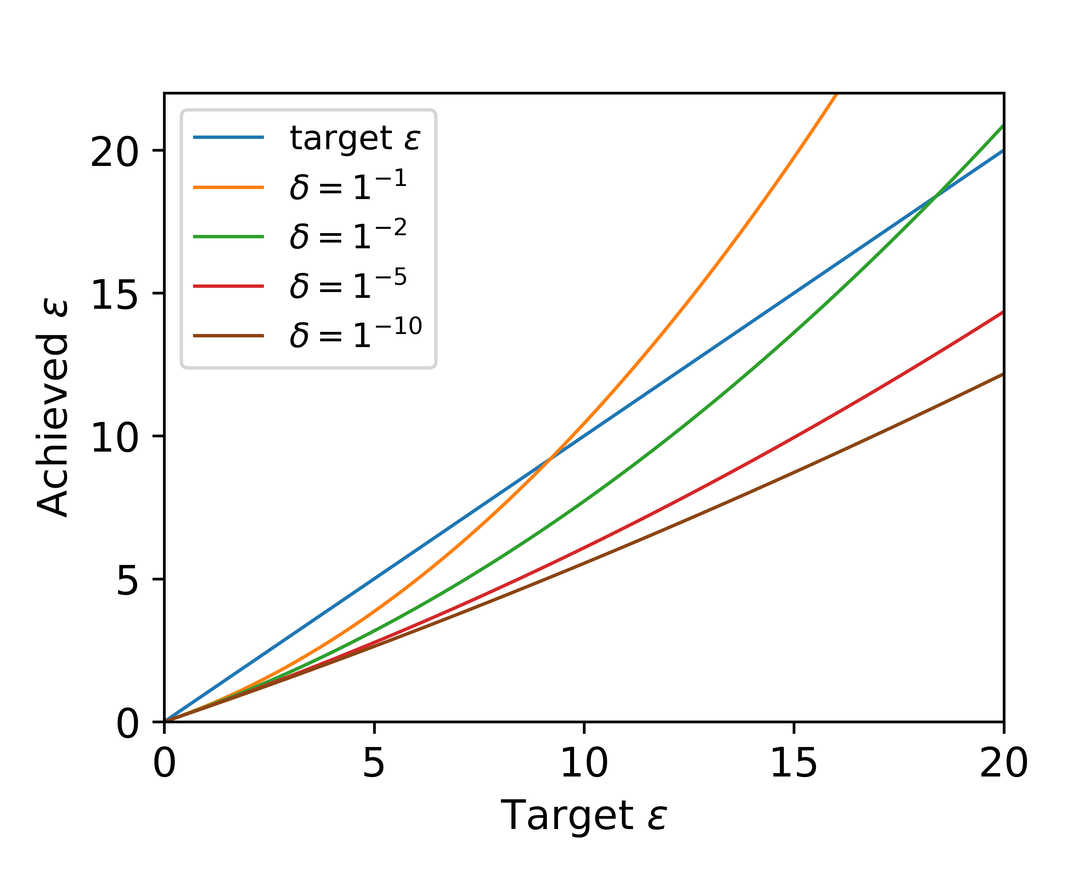
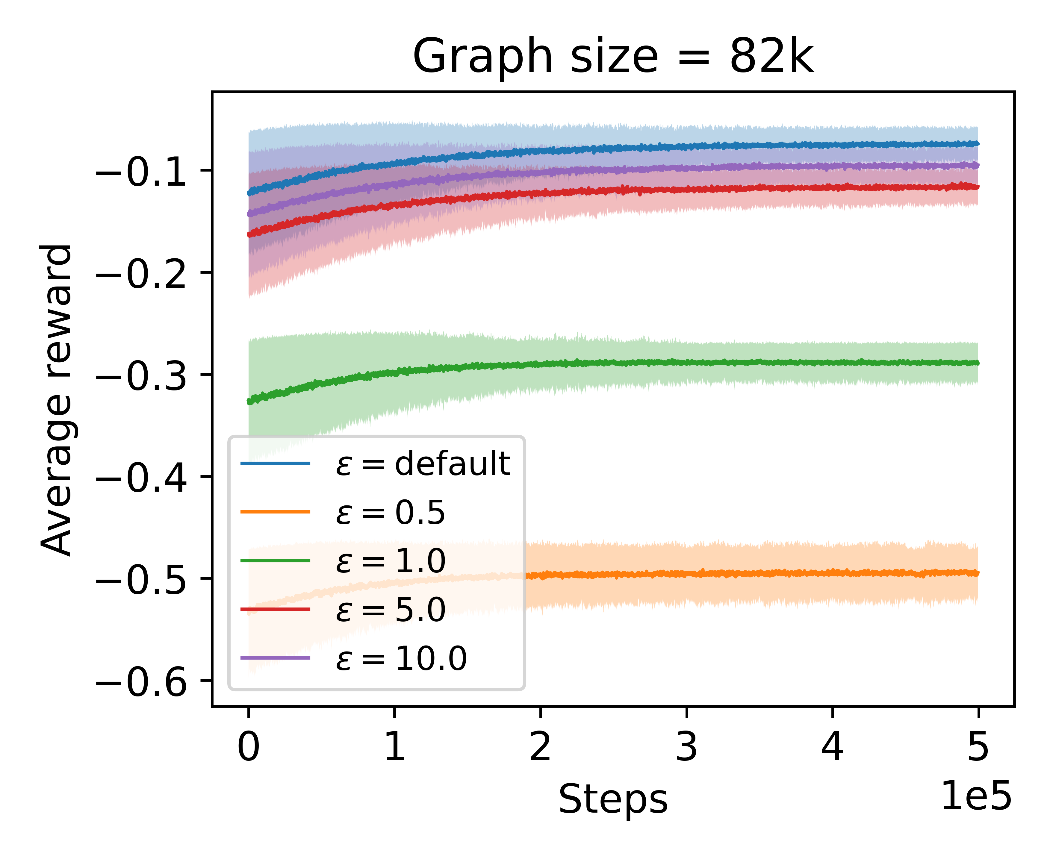
Figure 3: Left: Target privacy vs privacy achieved under equations (5) and (8) as $\delta$ is varied. $T=5e5$. Right: DP-DQN performance as $\epsilon$ is varied on graphs with 82K and 196K nodes.

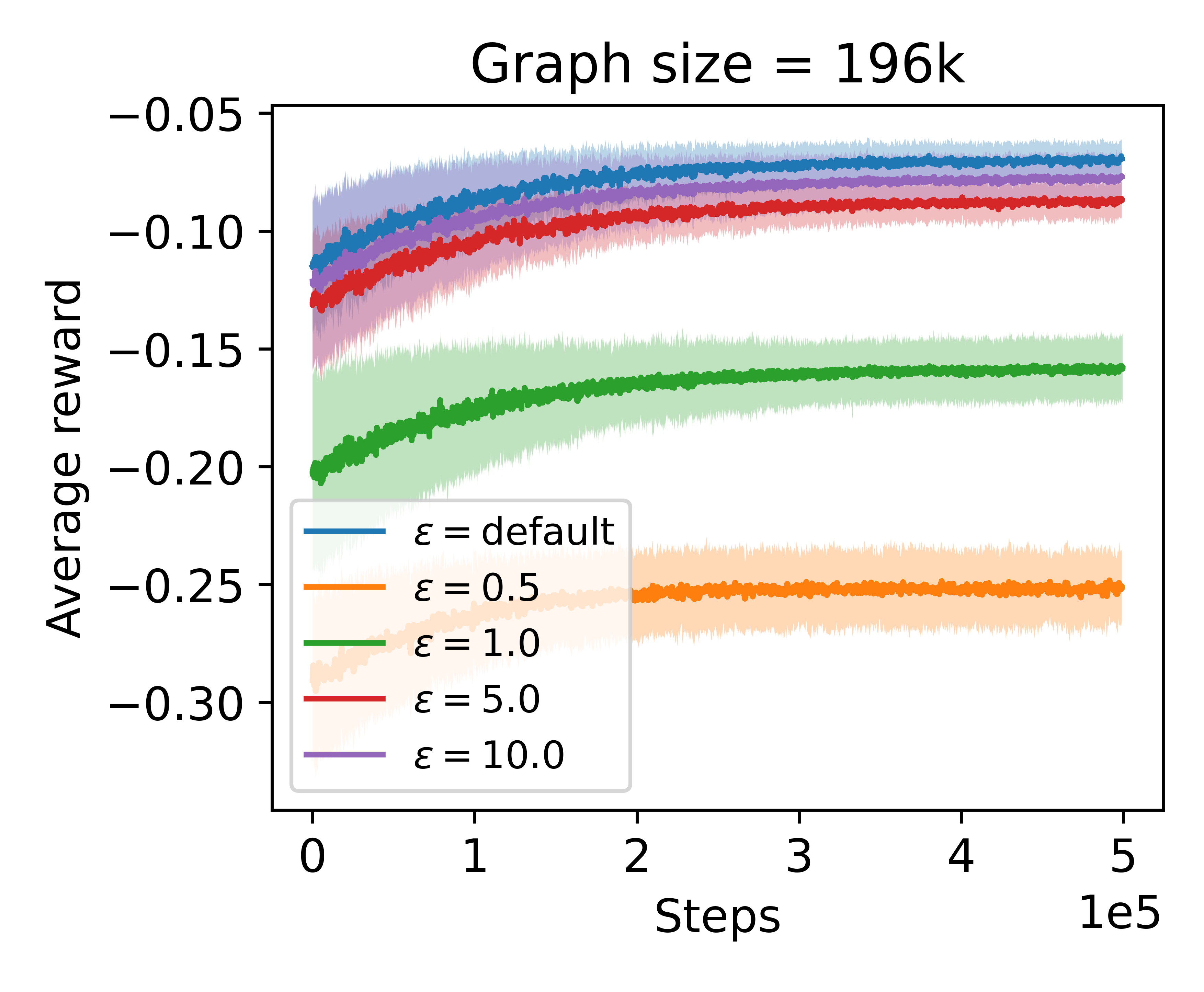
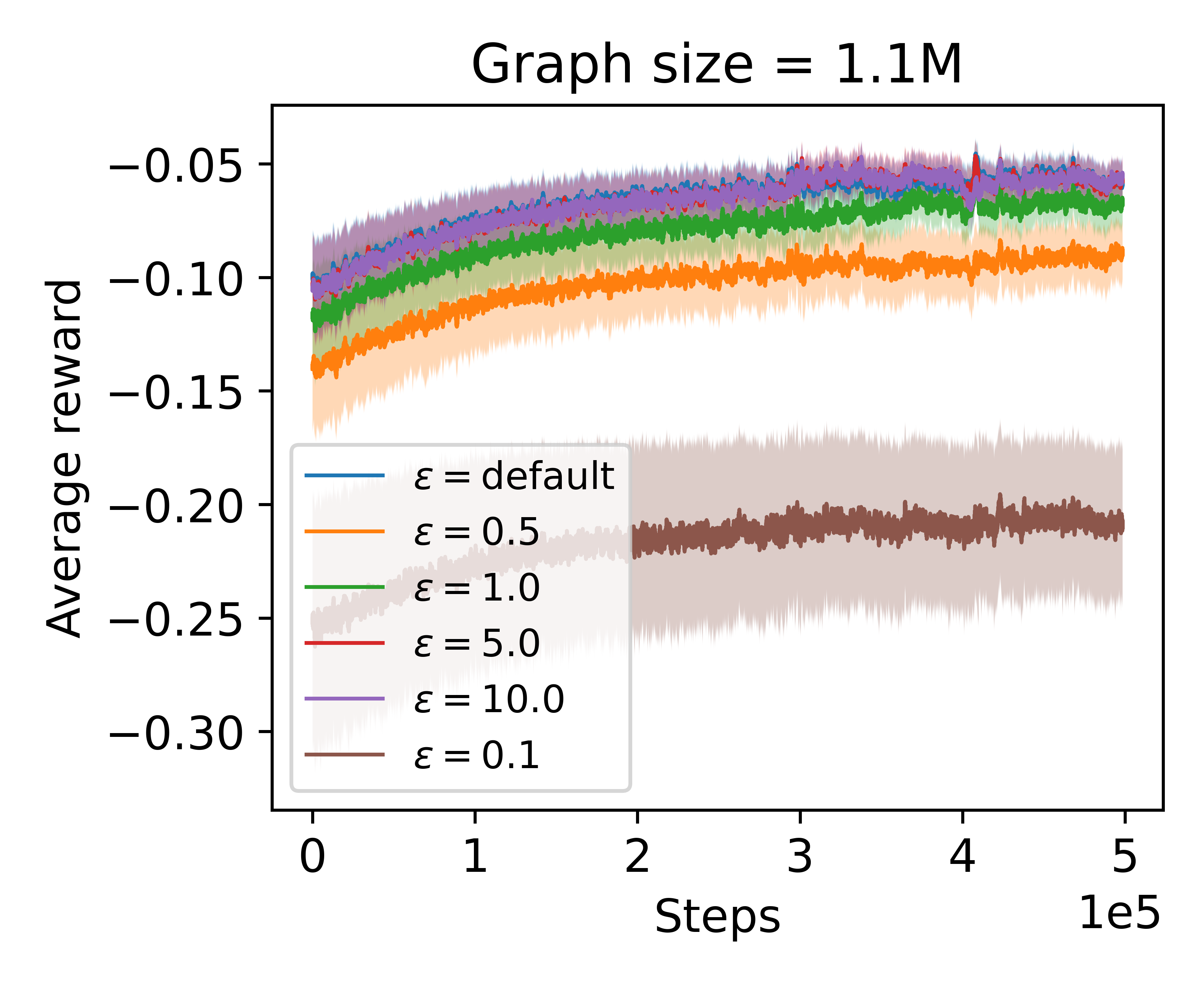
Figure 4: DP-DQN performance as $\epsilon$ is varied on graphs with 82K and 196K nodes.

The empirical results demonstrate in a finite sample setting the relationship between performance and the population size and privacy parameters highlighted by Theorem 3. For all graphs, the performance of DP-DQN in a low privacy setting (i.e. $\epsilon\geq 5$) clustered closely to the optimal performance. Notably, DP-DQN’s performance under low privacy on the 1.1M graph is essentially indistinguishable to the default performance. Across all graphs, the performance of DP-DQN degrades in a high privacy setting (i.e. $\epsilon<1$). The effect is especially pronounced for the small 81k graph. The performance of DP-DQN under $\epsilon=0.5$ in the 1.1M graph is quite close to the default performance. This falls in line with intuition as the noise added under a given privacy parameter has absolute scale. As the population size increases, the relative error due to privacy is much smaller. Assuming the environment transition function and reward function are Lipschitz, the small relative error due to privacy would not impact performance in a large population as much as it would in a smaller population. On the 1.1M graph we also plot the performance of DP-DQN under $\epsilon=0.1$. Again, this is made possible due to the increased population size.

6 Limitations and Future Work

One limitation of our theoretical results is that they are asymptotic in nature. This analysis provides guarantees on the error between the solution under privacy and the true solution without privacy, but does not provide any guidance on whether such a solution can be learned. Nevertheless, our empirical results provide some confidence the solutions found by learning algorithms will scale the way our results predict. Also, understanding the asymptotic properties of a problem setting is an important first step. Constructing and proving sublinear-regret algorithms in our problem setting is important future work.

Whilst our approach to achieving differential privacy is desirable as it is agnostic to the RL algorithm itself, it leaves open the possibility that the same privacy guarantees could be achieved by directly modifying an RL algorithm. Such an approach may be able to better deal with higher dimensional state spaces, which can adversely impact the approximation error, and is one of the limitations of our approach. Our analysis is also performed under some regularity assumptions; removing these assumptions would provide more generally applicable theoretical guarantees and is an interesting topic for future research.

Impact Statement

As reinforcement learning algorithms see wider adoption and begin interacting with humans and their data, issues around protecting privacy become more pertinent. Our work can be seen as providing a promising start and solid theoretical foundation to providing privacy protections in an important problem class where reinforcement learning may be applied in the future.

Acknowledgements

The authors would like to thank Mike Purcell for the many helpful discussions and whiteboard sessions during the development of the work.

Appendix

Appendix A Proof of Lemma 1

Lemma 1.

A family of mechanisms $\mathcal{F}$ satisfies $(\epsilon,\delta)$-differential privacy under $T$-fold adaptive composition iff every sequence of mechanisms $\mathcal{M}=(\mathcal{M}_{1},\ldots,\mathcal{M}_{T})$, with $\mathcal{M}_{i}\in\mathcal{F}$, satisfies $(\epsilon,\delta)$-Pufferfish privacy with parameters $(\mathbb{S},\mathbb{Q},\Theta)$ as defined in Section 3.2.

Proof.

We first show $T$-fold adaptive composition implies $(\epsilon,\delta)$-Pufferfish privacy.

Suppose $\mathcal{M}=(\mathcal{M}_{1},\ldots,\mathcal{M}_{T})$ satisfies $(\epsilon,\delta)$ differential privacy under $T$-fold adaptive composition. Let $\mathfrak{D}_{1:T}$ be a random variable denoting the sequence of databases. Given an arbitrary $\theta$, secret $\sigma_{i,S}$, we have for each non-empty $R\subseteq S$,

$$P(\mathcal{M}(\mathfrak{D}_{1:T})=y_{1:T}\,|\,\sigma_{(i,S)},\theta)$$ (9)

$$=\sum_{G_{1:T}}\sum_{X_{1:T}}\sum_{D_{1:T}\,|\,\sigma_{(i,S)}}P(G_{1:T},X_{1:T}\,|\,\theta)P(\mathfrak{D}_{1:T}=D_{1:T}\,|\,G_{1:T},X_{1:T},\sigma_{(i,S)},\theta)P(\mathcal{M}(D_{1:T})=y_{1:T})$$

$$\leq\delta+e^{\epsilon}\sum_{G_{1:T}}\sum_{X_{1:T}}\sum_{D_{1:T}\,|\,\sigma_{(i,S)}}P(G_{1:T},X_{1:T}\,|\,\theta)P(\mathfrak{D}_{1:T}=D_{1:T}\,|\,G_{1:T},X_{1:T},\sigma_{(i,S)},\theta)P(\mathcal{M}(D^{\prime}_{1:T})=y_{1:T}),$$

where $D^{\prime}_{1:T}$ is obtained from $D_{1:T}$ by removing individual $i$’s data from $D_{t}$, $t\in R$. The inequality (9) follows from the property of T-fold adaptive composition:

$$\max_{\omega:P(\mathcal{M}(D_{1:T})=\omega)\geq\delta}\ln\frac{P(\mathcal{M}(D_{1:T})=\omega)-\delta}{P(\mathcal{M}(D^{\prime}_{1:T})=\omega)}\leq\epsilon.$$ (10)

Given a $D_{1:T}$ satisfying $\sigma_{(i,S)}$, we have

$$P(\mathfrak{D}_{1:T}=D_{1:T} \,|\,G_{1:T},X_{1:T},\sigma_{(i,S)},\theta)=\biggl{[}\,\prod_{t\in S}P(\mathfrak{D}_{t}=D_{t}\,|\,X_{t},i\in L_{t},\theta)\biggr{]}\biggl{[}\,\prod_{t\in T\setminus S}P(\mathfrak{D}_{t}=D_{t}\,|\,X_{t},i\notin L_{t},\theta)\biggr{]}.$$

Given $D^{\prime}_{1:T}$ is obtained from $D_{1:T}$ as described above, it satisfies $\sigma_{(i,S\setminus R)}$ and we have

$$P( \mathfrak{D}_{1:T}=D^{\prime}_{1:T}\,|\,G_{1:T},X_{1:T},\sigma_{(i,S\setminus R)},\theta)=$$

$$\biggl{[}\,\prod_{t\in R}P(\mathfrak{D}_{t}=D^{\prime}_{t}\,|\,X_{t},i\neq L_{t},\theta)\biggr{]}\biggl{[}\,\prod_{t\in S\setminus R}P(\mathfrak{D}_{t}=D_{t}\,|\,X_{t},i\in L_{t},\theta)\biggr{]}\biggl{[}\,\prod_{t\in T\setminus S}P(\mathfrak{D}_{t}=D_{t}\,|\,X_{t},i\notin L_{t},\theta)\biggr{]}.$$

For each $t\in R$, we have

$$P(\mathfrak{D}_{t}=D_{t}\,|\,X_{t},i\in L_{t},\theta)=P(\mathfrak{D}_{t}=D^{\prime}_{t}\,|\,X_{t},i\notin L_{t},\theta)$$ (11)

since, by Equation (4), both the LHS and RHS of (11) are equal to

$$\prod_{j\in L_{t}\setminus\{i\}}\mu_{t,j}\prod_{j\in[N^{*}]\setminus L_{t}\}}(1-\mu_{t,j}).$$

We have thus established that

$$P(\mathfrak{D}_{1:T}=D_{1:T}\,|\,G_{1:T},X_{1:T},\sigma_{(i,S)},\theta)=P(\mathfrak{D}_{1:T}=D^{\prime}_{1:T}\,|\,G_{1:T},X_{1:T},\sigma_{(i,S\setminus R)},\theta).$$ (12)

Substituting Equation (12) into (9), and noting that the innermost summation $\sum_{D_{1:T}\,|\,\sigma_{(i,S)}}$ in (9) can be rewritten in the equivalent form $\sum_{D^{\prime}_{1:T}\,|\,\sigma_{(i,S\setminus R)}}$, allows us to claim

$$P(\mathcal{M}(\mathfrak{D}_{1:T})=y_{1:T}\,|\,\sigma_{(i,S)},\theta)\leq\delta+e^{\epsilon}P(\mathcal{M}(\mathfrak{D}_{1:T})=y_{1:T}\,|\,\sigma_{(i,S\setminus R)},\theta).$$

Given $\theta\in\Theta,i\in[N^{*}],S\subseteq[T]$ and $R\subseteq S$ are all arbitrary, we have shown $\mathcal{M}$ satisfies $(\epsilon,\delta)$-Pufferfish privacy with parameters $(\mathbb{S},\mathbb{Q},\Theta)$.

We next show $(\epsilon,\delta)$-Pufferfish privacy implies $T$-fold adaptive composition.

Suppose $\mathcal{M}=(\mathcal{M}_{1},\ldots,\mathcal{M}_{T})$ satisfies $(\epsilon,\delta)$ Pufferfish privacy with parameters $(\mathbb{S},\mathbb{Q},\Theta)$. We show for any pair of neighbouring databases there is a $\theta\in\Theta$ that preserves differential privacy.

Let $D_{1:T}$ be an arbitrary sequence of datasets. For each individual $i$ in $D_{1:T}$, let $D^{\prime}_{1:T}$ be obtained from $D_{1:T}$ by removing individual $i$’s data from one or more of the datasets. Thus, there exists $S$ and $R\subseteq S$ such that $D_{1:T}$ satisfies $\sigma_{(i,S)}$ and $D^{\prime}_{1:T}$ satisfies $\sigma_{(i,S\setminus R)}$.

We choose $\theta=\{(\mathscr{E},\mu_{t,1},\ldots,\mu_{t,N^{*}}\}_{t=1..T}$ to be the following. $\mathscr{E}$ can be any stochastic population process. For each $t\in S$, define $\mu_{t,i}=1/2$, and $\mu_{t,j}=1$ for each $j\in L_{t}\setminus S$ and $\mu_{t,k}=0$ for each $k\notin L_{t}$. And for each $t\notin S$, define $\mu_{t,j}=1$ for each $j\in L_{t}$ and $\mu_{t,k}=0$ for each $k\notin L_{t}$. Given $\mathcal{M}$ satisfies $(\epsilon,\delta)$ Pufferfish privacy, we have for any $y_{1:T}$:

$$P(\mathcal{M}(\mathfrak{D}_{1:T})=y_{1:T}\,|\,\sigma_{(i,S)},\theta)\leq e^{\epsilon}P(\mathcal{M}(\mathfrak{D}_{1:T})=y_{1:T}\,|\,\sigma_{(i,S\setminus R)},\theta)+\delta$$ (13)

$$\Leftrightarrow\, P(\mathcal{M}(D_{1:T})=y_{1:T}\,|\,\sigma_{(i,S)},\theta)\leq e^{\epsilon}P(\mathcal{M}(D^{\prime}_{1:T})=y_{1:T}\,|\,\sigma_{(i,S\setminus R)},\theta)+\delta$$ (14)

$$\Leftrightarrow\, P(\mathcal{M}(D_{1:T})=y_{1:T}\,|\,\theta)\leq e^{\epsilon}P(\mathcal{M}(D^{\prime}_{1:T})=y_{1:T}\,|\,\theta)+\delta$$ (15)

Step (14) follows because of all the dataset sequences that can be generated using $\theta$, only $D_{1:T}$ satisfies $\sigma_{(i,S)}$ and only $D^{\prime}_{1:T}$ satisfies $\sigma_{(i,S\setminus R)}$. Step (15) follows because $P(\sigma_{(i,S)}\,|\,\theta)=P(\sigma_{(i,S\setminus R)}\,|\,\theta)=(1/2)^{|S|}$.

Choosing $\theta\in\Theta$ in this manner for all neighbouring database sequences and repeating the calculations proves the final result. ∎

In the proof of Lemma 1, we have only considered neighbouring datasets where an individual’s data is dropped. The case when a neighbouring dataset $D^{\prime}$ is obtained from a dataset $D$ by replacing an individual $i$’s data with another individual $j$’s data, where $j$ is not in $D$, can be formulated using the following secrets and secret pairs:

$$\sigma_{(i,S)} \coloneqq\biggl{(}\,\bigwedge_{t\in S}\,i\in L_{t}\biggr{)}\wedge\biggl{(}\,\bigwedge_{t\in[T]\setminus S}i\notin L_{t}\biggr{)}$$

$$\sigma_{(i,S(W))} \coloneqq\biggl{(}\,\bigwedge_{t\in S\setminus W_{|1}}\,i\in L_{t}\biggr{)}\wedge\biggl{(}\,\bigwedge_{t\in[T]\setminus(S\setminus W_{|1})}i\notin L_{t}\biggr{)}\wedge\biggl{(}\,\bigwedge_{(t,j)\in W}j\in L_{t}\biggr{)}$$

$$\mathbb{S^{\prime}} \coloneqq\bigcup_{i\in[N^{*}]}\bigcup_{S\subseteq[T]:|S|\geq 1}\{\sigma_{(i,S)}\}$$

$$\mathbb{Q^{\prime}} \coloneqq\bigcup_{i\in[N^{*}]}\bigcup_{S\subseteq[T]:|S|\geq 1}\,\bigcup_{\begin{subarray}{c}W=\{(t,j)\,:\,t\in R,j\in[N^{*}]\setminus S\}\\ R\subseteq S\wedge|R|\geq 1\end{subarray}}\{(\sigma_{(i,S)},\sigma_{(i,S(W))}\}$$

In the above, given $W=\{(t,x)\}$, we define $W_{|1}=\{t\,:\,\exists x.(t,x)\in W\}$. Using very similar arguments, one can show that $(\epsilon,\delta)$ differential privacy under T-fold adaptive composition is equivalent to $(\epsilon,\delta)$ Pufferfish privacy with parameters $(\mathbb{S^{\prime}},\mathbb{Q^{\prime}},\Theta)$.

For each of the secret pairs $(s_{1},s_{2})\in\mathbb{Q^{\prime}}$, the Pufferfish privacy guarantees that

$$e^{-\epsilon}\leq\frac{P(s_{1}\,|\,\mathcal{M}(\mathfrak{D}_{1:T})=\omega,\theta)}{P(s_{2}\,|\,\mathcal{M}(\mathfrak{D}_{1:T})=\omega,\theta)}\bigg{/}\frac{P(s_{1}\,|\,\theta)}{P(s_{2}\,|\,\theta)}\leq e^{\epsilon}.$$ (16)

By inspecting the proof of Lemma 1, it is clear that secret pairs that represent an individual having two different status at a given time cannot be accommodated, and this is consistent with Example 4.

Appendix B Utility Analysis Proofs

B.1 Laplace and Projected Laplace Mechanism Properties

The mechanism we consider using is the projected laplace mechanism. Denote by $\mathcal{M}_{L}$ the laplace mechanism which outputs ${s^{\prime}=\mathcal{M}_{L}(s)=s+(Y_{1},\ldots,Y_{K})}$, $Y_{i}\sim Lap(\Delta q/\epsilon)$. The projected laplace mechanism outputs $\tilde{s}=\mathcal{M}(s)$ by first applying the laplace mechanism $s^{\prime}=\mathcal{M}_{L}(s)$ and then takes the $\ell_{2}$ projection back onto the state space, i.e. $\tilde{s}=\arg\min_{\tilde{s}\in\mathcal{S}}\left\lVert\tilde{s}-s^{\prime}\right\rVert_{2}$.

A concentration bound for the Laplace mechanism is given as follows.

Theorem 4 (Dwork & Roth (2014)).

Let $X_{t}=(X_{t,i})_{i\in L_{t}}$ denote a dataset, $s=q(X_{t})$ and $s^{\prime}=\mathcal{M}_{L}(s)$. For $\epsilon>0$ and $\delta\in(0,1]$,

$$\mathbb{P}\left[\left\lVert s-s^{\prime}\right\rVert_{\infty}\geq\ln\left(\frac{K}{\delta}\right)\cdot\left(\frac{\Delta q}{\epsilon}\right)\right]\leq\delta.$$

The following is a simple corollary of Theorem 4.

Corollary 1.

Let $X_{t}=(X_{t,i})_{i\in L_{t}}$ denote a dataset and let $s=q(X_{t})$ and $s^{\prime}=\mathcal{M}_{L}(s)$. Then for $\epsilon>0$ and $\alpha>0$,

$$\mathbb{P}\left(\left\lVert s-s^{\prime}\right\rVert_{\infty}\geq\alpha\right)\leq K\exp\left(-\frac{N\alpha\epsilon}{2}\right).$$

We now prove Theorem 2, a concentration bound for the projected laplace mechanism.

Theorem 2.

Let $X_{t}=(X_{t,i})_{i\in L_{t}}$ denote a dataset and let $s=q(X_{t})$ and $\tilde{s}=\mathcal{M}(s)$, where $\mathcal{M}$ is the Projected Laplace mechanism. Then for all $\epsilon>0$ and $\alpha>0$,

$$\mathbb{P}\left(\left\lVert s-\tilde{s}\right\rVert_{\infty}\geq\alpha+\frac{1}{\sqrt{2}N}\right)\leq K\exp\left(-\frac{N\alpha\epsilon}{2\sqrt{K}}\right).$$

Proof.

First, define $P_{\Delta_{K}}(s)=\arg\min_{s^{\prime}\in\Delta_{K}}\left\lVert s^{\prime}-s\right\rVert_{2}$ and $P_{\mathcal{S}}(s)=\arg\min_{s^{\prime}\in\mathcal{S}}\left\lVert s^{\prime}-s\right\rVert_{2}$ as the $\ell_{2}$ projections onto the $K-1$ probability simplex $\Delta_{K}$ and the state space $\mathcal{S}$, noting that $\mathcal{S}\subset\Delta_{K}$. Letting $s^{\prime}=\mathcal{M}_{L}(s)$, we can express $\tilde{s}$ as $\tilde{s}=\mathcal{M}(s)=P_{\mathcal{S}}(s^{\prime})$.

Rather than finding an upper bound on $\mathbb{P}(\left\lVert s-\tilde{s}\right\rVert_{\infty}\geq\alpha)$, we instead find a lower bound on $\mathbb{P}(\left\lVert s-\tilde{s}\right\rVert_{\infty}<\alpha)$. Note that the $\ell_{\infty}$ ball of radius $\alpha$ (actually a hypercube) has greater volume than the $\ell_{2}$ ball of radius $\alpha$. Thus,

$$\mathbb{P}\left(\left\lVert s-\tilde{s}\right\rVert_{\infty}<\alpha\right)\geq\mathbb{P}\left(\left\lVert s-\tilde{s}\right\rVert_{2}<\alpha\right).$$ (17)

Now define the following sets:

$$A \coloneqq\left\{s^{\prime}\in\mathbb{R}^{K}:\left\lVert s-P_{\mathcal{S}}(s^{\prime})\right\rVert_{2}<\alpha+\frac{1}{\sqrt{2}N}\right\}$$

$$B \coloneqq\left\{s^{\prime}\in\mathbb{R}^{K}:\left\lVert s-P_{\Delta_{K}}(s^{\prime})\right\rVert_{2}<\alpha\right\}$$

Note that $P_{\mathcal{S}}(s^{\prime})$ must be a point that minimizes the $\ell_{2}$ distance to $P_{\Delta_{K}}(s^{\prime})$, as $P_{\Delta_{K}}(s^{\prime})$ is the minimum distance to the simplex $\Delta_{K}$ and minimizing the distance to $\mathcal{S}$ thus involves minimizing the distance along $\Delta_{K}$ from $P_{\Delta_{K}}(s^{\prime})$. Also for two neighbouring points $s_{1},s_{2}\in\mathcal{S}$ (i.e. $s_{1}\neq s_{2}$ and closest in $\ell_{2}$ distance), we must have two dimensions $i\neq j$ where $s_{1,i}=s_{2,i}-\frac{1}{N}$ and $s_{1,j}=s_{2,i}+\frac{1}{N}$ and $s_{1,k}=s_{2,k}$ for $k\neq i,j$. Thus the minimum distance between two neighbouring points is $\left\lVert s_{1}-s_{2}\right\rVert_{2}=\frac{\sqrt{2}}{N}$ and $P_{\mathcal{S}}(s^{\prime})$ can be at most $\frac{1}{\sqrt{2}N}$ away from $P_{\Delta_{K}}(s^{\prime})$. Then for $s^{\prime}\in B$, we have:

$$\left\lVert s-P_{\mathcal{S}}(s^{\prime})\right\rVert_{2} \leq\left\lVert s-P_{\Delta_{K}}(s^{\prime})\right\rVert_{2}+\left\lVert P_{\Delta_{K}}(s^{\prime})-P_{\mathcal{S}}(s^{\prime})\right\rVert_{2}$$

$$\leq\alpha+\frac{1}{\sqrt{2}N}.$$

Thus $s^{\prime}\in B\implies s^{\prime}\in A$, implying $B\subseteq A$ and giving us $\mathbb{P}(A)\geq\mathbb{P}(B)$ or equivalently:

$$\mathbb{P}\left(\left\lVert s-P_{\mathcal{S}}(s^{\prime})\right\rVert_{2}<\alpha+\frac{1}{\sqrt{2}N}\right)\geq\mathbb{P}\left(\left\lVert s-P_{\Delta_{K}}(s^{\prime})\right\rVert_{2}<\alpha\right).$$ (18)

Let $\theta\in[0,\frac{\pi}{2}]$ denote the angle between $s-s^{\prime}$ and the plane $\Delta_{K}$. Since $P_{\Delta_{K}}(s^{\prime})$ is the orthogonal projection, we have $\left\lVert s-s^{\prime}\right\rVert_{2}=\left\lVert s-P_{\Delta_{K}}(s^{\prime})\right\rVert_{2}\cos^{-1}(\theta)$. Then we have:

$$\mathbb{P}\left(\left\lVert s-P_{\Delta_{K}}(s^{\prime})\right\rVert_{2}<\alpha\right) =\mathbb{P}\left(\left\lVert s-s^{\prime}\right\rVert_{2}<\alpha\cos^{-1}(\theta)\right)$$

$$\overset{(a)}{\geq}\mathbb{P}\left(\left\lVert s-s^{\prime}\right\rVert_{\infty}<\frac{\alpha\cos^{-1}(\theta)}{\sqrt{K}}\right)$$

$$=1-\mathbb{P}\left(\left\lVert s-s^{\prime}\right\rVert_{\infty}\geq\frac{\alpha\cos^{-1}(\theta)}{\sqrt{K}}\right)$$

$$\overset{(b)}{\geq}1-K\exp\left(-\frac{N\alpha\epsilon\cos^{-1}(\theta)}{2\sqrt{K}}\right),$$ (19)

where (a) follows as $\{s^{\prime}\in\mathbb{R}^{K}:\left\lVert s-s^{\prime}\right\rVert_{\infty}\leq\alpha/\sqrt{K}\}\subseteq\{s^{\prime}\in\mathbb{R}^{K}:\left\lVert s-s^{\prime}\right\rVert_{2}\leq\alpha\}$ – the former is a hypercube with side length $2\alpha/\sqrt{K}$ sitting completely inside the $\ell_{2}$ ball of radius $\alpha$ – and (b) follows by Corollary 1.

Combining (17), (18) and (19) then gives us:

$$\mathbb{P}\left(\left\lVert s-\tilde{s}\right\rVert_{\infty}<\alpha+\frac{1}{\sqrt{2}N}\right)\geq 1-K\exp\left(-\frac{N\alpha\epsilon}{2\sqrt{K}}\right),$$

where we drop $\cos^{-1}(\theta)$ as $\cos^{-1}(\theta)\in[1,\infty]$ for $\theta\in[0,\frac{\pi}{2}]$. Thus, we have:

$$\mathbb{P}\left(\left\lVert s-\tilde{s}\right\rVert_{\infty}\geq\alpha+\frac{1}{\sqrt{2}N}\right) =1-\mathbb{P}\left(\left\lVert s-\tilde{s}\right\rVert_{\infty}<\alpha+\frac{1}{\sqrt{2}N}\right)$$

$$\leq K\exp\left(-\frac{N\alpha\epsilon}{2\sqrt{K}}\right).$$

∎

B.2 Additional Lemmas

The Simulation Lemma Kearns & Singh (2002); Agarwal et al. (2022) lets us bound the value function error in terms of the error in the transition functions.

Lemma 4 (Simulation Lemma).

Let $M=(\mathcal{S},\mathcal{A},r,P,\gamma)$ and $\tilde{M}=(\mathcal{S},\mathcal{A},r,\tilde{P},\gamma)$ be two MDPs that differ only in the transition model. Given a policy $\pi$, let $Q^{\pi}$ be the value function under $\pi$ in $M$ and $\tilde{Q}^{\pi}$ be the value function under $\pi$ in $\tilde{M}$. Then for all $\pi$

$$\left\lVert Q^{\pi}-\tilde{Q}^{\pi}\right\rVert_{\infty}\leq\frac{\gamma}{1-\gamma}\left\lVert(P-\tilde{P})V^{\pi}\right\rVert_{\infty}.$$

Lemma 5 (Lipschitz preservation under convolution).

Suppose $f$ is an $L$-Lipschitz function and $\phi$ is a function such that $\int\phi(x)dx=1$ and $\phi(x)\geq 0$ for all $x$. Then $g=f\ast\phi$ is also an $L$-Lipschitz function.

Proof.

$$\left\lVert g(z)-g(z^{\prime})\right\rVert \leq\left\lVert\int(f(z+x)-f(z^{\prime}+x))\phi(x)dx\right\rVert$$

$$\leq\int\left\lVert f(z+x)-f(z^{\prime}+x)\right\rVert\phi(x)dx$$

$$\leq L\left\lVert z-z^{\prime}\right\rVert\int\phi(x)dx$$

$$=L\left\lVert z-z^{\prime}\right\rVert~{}.$$

∎

B.3 Proof of Theorem 3

Theorem 3.

Let $M$ be the MDP environment and $\tilde{M}$ denote the privatised MDP under an $\epsilon$-differentially private projected laplace mechanism. Let $Q^{*}$ be the optimal value function in $M$ and $\tilde{Q}^{*}$ be the optimal value function in $\tilde{M}$. Then,

$$\left\lVert Q^{*}-\tilde{Q}^{*}\right\rVert_{\infty} \leq\mathcal{O}\left(\sqrt{K}\exp\left(-\frac{\epsilon}{2\sqrt{2K}}\right)+K\exp\left(-\sqrt{N}\epsilon\right)+\frac{K^{\frac{3}{2}}}{\sqrt{N}}\right).$$

Proof.

We have

$$\left\lvert Q^{*}(s,a)-\tilde{Q}^{*}(s,a)\right\rvert =\left\lvert\sup_{\pi}Q^{\pi}(s,a)-\sup_{\pi}\tilde{Q}^{\pi}(s,a)\right\rvert$$

$$\leq\sup_{\pi}\left\lvert Q^{\pi}(s,a)-\tilde{Q}^{\pi}(s,a)\right\rvert$$

$$\leq\sup_{\pi}\left\lVert Q^{\pi}-\tilde{Q}^{\pi}\right\rVert_{\infty}.$$ (20)

Then (20) can be bound with Lemma 4. For any policy $\bar{\pi}$ and any behaviour policy $\pi$ satisfying Assumption 3,

$$\left\lVert Q^{\bar{\pi}}-\tilde{Q}^{\bar{\pi}}\right\rVert_{\infty} \leq\frac{\gamma}{1-\gamma}\left\lVert(P-\tilde{P}^{\pi})V^{\bar{\pi}}\right\rVert_{\infty}$$

$$\leq\frac{\gamma}{1-\gamma}\max_{s,a}\left\lVert P_{sa}-\tilde{P}^{\pi}_{sa}\right\rVert_{1}\left\lVert V^{\bar{\pi}}\right\rVert_{\infty}$$

$$\leq\frac{\gamma r_{\max}}{(1-\gamma)^{2}}\max_{s,a}\left\lVert P_{sa}-\tilde{P}^{\pi}_{sa}\right\rVert_{1}.$$ (21)

In the above, $\tilde{P}^{\pi}$ is as defined in (6) and denotes the transition model in $\tilde{M}$ under behaviour policy $\pi$. Writing $\bar{P}(s^{\prime}\,|\,s_{1},a)=\sum\limits_{s_{2}\in\mathcal{S}}P(s_{2}\,|\,s_{1},a)P_{\mathcal{M}}(s^{\prime}\,|\,s_{2})$, we have, for any $s,a$,

$$\left\lVert P_{sa}-\tilde{P}^{\pi}_{sa}\right\rVert_{1}=\left\lVert P_{sa}-\sum_{s_{1}\in\mathcal{S}}\nu_{\pi}(s_{1}\,|\,s,a)\bar{P}_{s_{1}a}\right\rVert_{1}$$

$$=\left\lVert\sum_{s_{1}\in\mathcal{S}}\nu_{\pi}(s_{1}\,|\,s,a)P_{sa}-\sum_{s_{1}\in\mathcal{S}}\nu_{\pi}(s_{1}\,|\,s,a)\bar{P}_{s_{1}a}\right\rVert_{1}$$

$$\leq\sum_{s_{1}\in\mathcal{S}}\nu_{\pi}(s_{1}\,|\,s,a)\left\lVert P_{sa}-\bar{P}_{s_{1}a}\right\rVert_{1}$$

$$\leq\sum_{s_{1}\in\mathcal{S}}\nu_{\pi}(s_{1}\,|\,s,a)\left(\underbrace{\left\lVert P_{sa}-\bar{P}_{sa}\right\rVert_{1}}_{(one)}+\underbrace{\left\lVert\bar{P}_{sa}-\bar{P}_{s_{1}a}\right\rVert_{1}}_{(two)}\right),$$

where the last two steps follows from the triangle inequality and splitting $\left\lVert P_{sa}-\bar{P}_{s_{1}a}\right\rVert_{1}$. The first term can be viewed as the error due to output privatisation and the second term can be viewed as the error due to input privatisation. We will look to bound the two terms separately.

Term (one)
By the Bretagnolle-Huber inequality Bretagnolle & Huber (1979); Canonne (2023), term (one) can be bound as:

$$\left\lVert P_{sa}-\bar{P}_{sa}\right\rVert_{1}\leq 2\sqrt{1-\exp(-D_{\mathit{KL}}(P_{sa}\,||\,\bar{P}_{sa})}.$$

The KL divergence term can be lower bound as follows:

$$-D_{\mathit{KL}}(P_{sa}\,||\,\bar{P}_{sa}) =\sum_{s^{\prime}\in\mathcal{S}}P_{sa}^{s^{\prime}}\log\frac{\bar{P}_{sa}^{s^{\prime}}}{P_{sa}^{s^{\prime}}}$$

$$=\sum_{s^{\prime}\in\mathcal{S}}P_{sa}^{s^{\prime}}\log\frac{\sum_{s_{2}\in\mathcal{S}}P_{\mathcal{M}}(s^{\prime}\,|\,s_{2})P_{sa}^{s_{2}}}{P_{sa}^{s^{\prime}}}$$

$$\geq\sum_{s^{\prime}\in\mathcal{S}}P_{sa}^{s^{\prime}}\log\frac{P_{\mathcal{M}}(s^{\prime}\,|\,s^{\prime})P_{sa}^{s^{\prime}}}{P_{sa}^{s^{\prime}}}$$ (22)

$$=\sum_{s^{\prime}\in\mathcal{S}}P_{sa}^{s^{\prime}}\log P_{\mathcal{M}}(s^{\prime}\,|\,s^{\prime})$$

$$\geq\min_{s^{\prime}\in\mathcal{S}}\log P_{\mathcal{M}}(s^{\prime}\,|\,s^{\prime}).$$

Here (22) follows as we shrink the sum to just when $s_{2}=s^{\prime}$.

Note that $P_{\mathcal{M}}(s^{\prime}\,|\,s^{\prime})$ is smallest when $s^{\prime}$ is an interior point as it has the smallest subspace of $\mathbb{R}^{K}$ that projects back onto itself. So let $s^{\prime}\in\mathcal{S}\setminus\partial\mathcal{S}$ denote an interior point going forward. Thus term (one) can be bound as:

$$\left\lVert P_{sa}-\bar{P}_{sa}\right\rVert_{1} \leq 2\sqrt{1-P_{\mathcal{M}}(s^{\prime}\,|\,s^{\prime})}.$$ (23)

We now look to lower bound $P_{\mathcal{M}}(s^{\prime}\,|\,s^{\prime})$. Letting $\mathcal{R}(s^{\prime})$ denote the subspace that projects onto $s^{\prime}$, $P_{\mathcal{M}}(s^{\prime}\,|\,s^{\prime})$ can be expressed as

$$P_{\mathcal{M}}(s^{\prime}\,|\,s^{\prime}) =P_{\mathcal{M}_{L}}(s\in\mathcal{R}(s^{\prime})\,|\,s^{\prime})$$

$$=\int_{s\in\mathcal{R}(s^{\prime})}\left(\frac{N\epsilon}{4}\right)^{K}\exp\left(-\frac{N\epsilon}{2}\left\lVert s-s^{\prime}\right\rVert_{1}\right)ds.$$

Let $\delta=\frac{1}{\sqrt{2}N}$ and $\mathcal{B}^{2}_{\delta}(s^{\prime})\coloneqq\{s\in\mathbb{R}^{K}:\left\lVert s-s^{\prime}\right\rVert_{2}\leq\delta\}$ denote the $\ell_{2}$ ball of radius $\delta$. Clearly, all points inside $\mathcal{B}^{2}_{\delta}(s^{\prime})$ are closest to $s^{\prime}$ compared to any other point in the state space. Also, we have that $\mathcal{B}^{2}_{\delta}(s^{\prime})\subseteq\mathcal{R}(s^{\prime})$. Integrating, we get:

$$P_{\mathcal{M}_{L}}(s\in\mathcal{R}(s^{\prime})\,|\,s^{\prime}) =\int_{s\in\mathcal{R}(s^{\prime})}\left(\frac{N\epsilon}{4}\right)^{K}\exp\left(-\frac{N\epsilon}{2}\left\lVert s-s^{\prime}\right\rVert_{1}\right)ds$$

$$\geq\int_{s\in\mathcal{B}_{\delta}^{2}(s^{\prime})}\prod_{i=1}^{K}\left(\frac{N\epsilon}{4}\right)\exp\left(-\frac{N\epsilon}{2}\left\lvert s_{i}-s^{\prime}_{i}\right\rvert\right)ds$$

Let $\delta_{K}=\delta/\sqrt{K}$. We now integrate over $C_{\delta_{K}}(x^{\prime})\coloneqq\bigtimes_{i=1}^{K}[s^{\prime}_{i}-\delta_{K},s^{\prime}_{i}+\delta_{K}]$ to get a lower bound as $C_{\delta_{K}}(x^{\prime})\subseteq\mathcal{B}_{\delta}^{2}(x^{\prime})$. The integral is then:

$$P_{\mathcal{M}_{L}}(s\in\mathcal{R}(s^{\prime})\,|\,s^{\prime}) \geq\int_{s\in\mathcal{B}_{\delta}^{2}(s^{\prime})}\prod_{i=1}^{K}\left(\frac{N\epsilon}{4}\right)\exp\left(-\frac{N\epsilon}{2}\left\lvert s_{i}-s^{\prime}_{i}\right\rvert\right)ds$$

$$\geq\int_{s\in C_{\delta_{K}}(s^{\prime})}\prod_{i=1}^{K}\left(\frac{N\epsilon}{4}\right)\exp\left(-\frac{N\epsilon}{2}\left\lvert s_{i}-s^{\prime}_{i}\right\rvert\right)ds$$

$$=\prod_{i=1}^{K}\int_{s^{\prime}_{i}-\delta_{K}}^{s^{\prime}_{i}+\delta_{K}}\frac{N\epsilon}{4}\exp\left(-\frac{N\epsilon}{2}\left\lvert s_{i}-s^{\prime}_{i}\right\rvert\right)ds_{i}$$

$$=\prod_{i=1}^{K}\int_{-\delta_{K}}^{\delta_{K}}\frac{N\epsilon}{4}\exp\left(-\frac{N\epsilon}{2}\left\lvert s_{i}\right\rvert\right)ds_{i}$$

$$=\prod_{i=1}^{K}\left(1-\exp(-\alpha\delta_{K})\right)$$ (24)

$$=\left(1-\exp\left(-\frac{\epsilon}{2\sqrt{2K}}\right)\right)^{K}$$

$$\geq 1-K\exp\left(-\frac{\epsilon}{2\sqrt{2K}}\right),$$ (25)

where step (24) follows by noting that for, all $\alpha>0$

$$\frac{\alpha}{2}\int_{-\delta_{K}}^{\delta_{K}}\exp\left(-\alpha\left\lvert x\right\rvert\right)dx=\alpha\left(\int_{0}^{\delta_{K}}\exp\left(-\alpha x\right)dx\right)=\alpha\left[\frac{1-\exp(-\alpha\delta_{K})}{\alpha}\right]=1-\exp(-\alpha\delta_{K})$$

and setting $\alpha=N\epsilon/2$, and step (25) follows by noting that for all $p\in[0,1]$, $(1-p)^{k}\geq 1-kp$.

Substituting into equation (23) gives the following bound on term (one):

$$\sum_{s_{1}\in\mathcal{S}}\nu_{\pi}(s_{1}\,|\,s,a)\left\lVert P_{sa}-\bar{P}_{sa}\right\rVert_{1} \leq 2\sqrt{1-P_{\mathcal{M}}(s^{\prime}\,|\,s^{\prime})}$$

$$=2\sqrt{1-\left(1-K\exp\left(-\frac{\epsilon}{2\sqrt{2K}}\right)\right)}$$

$$=2\sqrt{K}\exp\left(-\frac{\epsilon}{2\sqrt{2K}}\right).$$ (26)

Term (two)
Using equation 7, we have:

$$\sum_{s_{1}\in\mathcal{S}}\nu_{\pi}(s_{1}\,|\,s,a)\left\lVert\bar{P}_{sa}-\bar{P}_{s_{1}a}\right\rVert_{1} =\sum_{s_{1}\in\mathcal{S}}\frac{P_{\mathcal{M}}(s\,|\,s_{1})\nu_{\pi}(s_{1}\,|\,a)}{\tilde{\nu}_{\pi}(s\,|\,a)}\left\lVert\bar{P}_{sa}-\bar{P}_{s_{1}a}\right\rVert_{1}$$

$$\leq H\sum_{s_{1}\in\mathcal{S}}P_{\mathcal{M}}(s\,|\,s_{1})\left\lVert\bar{P}_{sa}-\bar{P}_{s_{1}a}\right\rVert_{1}$$

$$\leq H\sum_{s_{1}\in\mathcal{S}}\frac{P_{\mathcal{M}}(s\,|\,s_{1})}{P_{\mathcal{M}}(s_{1}\,|\,s)}P_{\mathcal{M}}(s_{1}\,|\,s)\left\lVert\bar{P}_{sa}-\bar{P}_{s_{1}a}\right\rVert_{1}$$

$$\leq HC_{\max}\sum_{s_{1}\in\mathcal{S}}P_{\mathcal{M}}(s_{1}\,|\,s)\left\lVert\bar{P}_{sa}-\bar{P}_{s_{1}a}\right\rVert_{1},$$

where $H=\max_{s,s_{1}}\frac{\nu_{\pi}(s_{1}\,|\,a)}{\tilde{\nu}_{\pi}(s\,|\,a)}$, and $C_{\max}=\max_{s,s_{1}}\frac{P_{\mathcal{M}}(s\,|\,s_{1})}{P_{\mathcal{M}}(s_{1}\,|\,s)}$.

We now look to bound $\sum_{s_{1}\in\mathcal{S}}P_{\mathcal{M}}(s_{1}\,|\,s)\left\lVert\bar{P}_{sa}-\bar{P}_{s_{1}a}\right\rVert_{1}$. For $\alpha>0$, define the $\ell_{\infty}$ ball of radius $\beta=\alpha+\frac{1}{\sqrt{2}N}$ around a state $s$ and its complement as:

$$B_{\alpha}(s) \coloneqq\{s^{\prime}\in\mathcal{S}:\left\lVert s-s^{\prime}\right\rVert_{\infty}<\beta\}$$

$$B_{\alpha}^{c}(s) \coloneqq\{s^{\prime}\in\mathcal{S}:\left\lVert s-s^{\prime}\right\rVert_{\infty}\geq\beta\}.$$

Splitting $\sum_{s_{1}\in\mathcal{S}}P_{\mathcal{M}}(s_{1}\,|\,s)\left\lVert\bar{P}_{sa}-\bar{P}_{s_{1}a}\right\rVert_{1}$ over $B_{\beta}(s)$ and $B_{\beta}^{c}(s)$ gives us the following bound:

$$\sum_{s_{1}\in\mathcal{S}} P_{\mathcal{M}}(s_{1}\,|\,s)\left\lVert\bar{P}_{sa}-\bar{P}_{s_{1}a}\right\rVert_{1}$$

$$=\sum_{s_{1}\in B_{\beta}(s)}P_{\mathcal{M}}(s_{1}\,|\,s)\left\lVert\bar{P}_{sa}-\bar{P}_{s_{1}a}\right\rVert_{1}+\sum_{s_{1}\in B^{c}_{\beta}(s)}P_{\mathcal{M}}(s_{1}\,|\,s)\left\lVert\bar{P}_{sa}-\bar{P}_{s_{1}a}\right\rVert_{1}$$

$$\leq LK\beta+2K\exp\left(-\frac{N\alpha\epsilon}{2\sqrt{K}}\right)$$ (27)

$$=2K\exp\left(-\frac{N\alpha\epsilon}{2\sqrt{K}}\right)+LK\alpha+\frac{LK}{\sqrt{2}{N}}.$$ (28)

The first term in inequality (27) follows by noting that $\bar{P}$ is $L$-Lipschitz by Lemma 5 and Assumption 2, and that, for all $x\in\mathbb{R}^{K}$, $\left\lVert x\right\rVert_{1}\leq K\left\lVert x\right\rVert_{\infty}$. The second term in inequality (27) follows by noting that the $L_{1}$ norm between distributions is bound by 2 and applying Proposition 2. Picking $\alpha=\frac{2\sqrt{K}}{\sqrt{N}}$ gives us

$$\sum_{s_{1}\in\mathcal{S}}P_{\mathcal{M}}(s_{1}\,|\,s)\left\lVert\bar{P}_{sa}-\bar{P}_{s_{1}a}\right\rVert_{1}\leq\mathcal{O}\left(K\exp\left(-\sqrt{N}\epsilon\right)+\frac{K^{3/2}}{\sqrt{N}}\right).$$

Thus the final bound on term (two) is:

$$\sum_{s_{1}\in\mathcal{S}}\nu_{\pi}(s_{1}\,|\,s,a)\left\lVert\bar{P}_{sa}-\bar{P}_{s_{1}a}\right\rVert_{1}\leq\mathcal{O}\left(K\exp\left(-\sqrt{N}\epsilon\right)+\frac{K^{3/2}}{\sqrt{N}}\right).$$ (29)

Combining (26) and (29) and picking the higher growth rate terms gives the final result. ∎

Appendix C Implementation Details

Our experimental results use a concrete instantiation of Algorithm 1 with DQN Mnih et al. (2015) and epsilon-greedy for exploration. We display the full algorithm details in Algorithm 3.

The state privatisation mechanism used is the projected laplace mechanism. We provide a particular instantiation of Algorithm 2 in Algorithm 4. Algorithm 4 works by first performing a projection onto the simplex using the sorting method from Shalev-Shwartz et al. (2006) before finding the nearest point in the state space. The sorting method has complexity $\mathcal{O}(K\log K)$ and finding the nearest point in the state space can be done in $\mathcal{O}(K)$.

Algorithm 3 has a few minor differences to Algorithm 1. Firstly, the algorithm takes the target cumulative privacy parameters as input instead of the per-step privacy parameters. The per-step privacy budget is calculated in line 5. Lines 10-21 of can be considered the RL algorithm in Algorithm 1 expanded. The replay buffer and target network are written such that they are not a part of the RL algorithm itself. This is done to make clear that the buffer and target network maintain state across all iterations. Finally, DQN returns a value function instead of a policy. This is a minor change however as the policy used is simply the epsilon-greedy policy with respect to the returned value function.

The parameters used in each experiment are listed in Table 3. The neural network used in all experiments was a 6 layer, fully connected MLP. The learning rate ($\alpha$) is not listed as we use the default settings of the RMSProp optimizer in PyTorch to optimize the neural network.

Algorithm 3 Differentially Private DQN (DP-DQN)

1:  Input: Environment $M=(\mathcal{S},\mathcal{A},r,P,\gamma)$, initial state $s_{0}\in\mathcal{S}$, privacy mechanism $\mathcal{M}:\mathcal{S}\times\mathbb{R}\to\mathcal{S}$.

2:  Parameters: cumulative privacy parameters $(\epsilon,\delta)$, time horizon $T$, batch size $B$, target update step $D$, population size $N$, learning rate $\alpha$, initial exploration rate $\epsilon_{start}<1$, decay rate $\kappa<1$.

3:  Initialize: network parameters $\theta$ randomly, target network parameters $\bar{\theta}=\theta$, $\epsilon_{explore}=\epsilon_{start}$.

4:  $\texttt{Buffer}\leftarrow\left\{\right\}$.

5:  $\epsilon^{\prime}=\frac{\epsilon}{2\sqrt{2T\log(1/\delta)}}$.

6:  $\tilde{s}_{0}=\mathcal{M}_{\epsilon^{\prime}}(s_{0})$.

7:  for $t=0,1,2,\ldots,T$ do

8:     $p\sim\mathit{Uniform}([0,1])$.

9:     if $p>\epsilon_{explore}$ then $\tilde{a}_{t}=\arg\max_{a}Q_{\theta}(\tilde{s}_{t},a)$ else $\tilde{a}_{t}\sim\mathit{Uniform}(\mathcal{A})$.

10:     Receive $s_{t+1}\sim P(\cdot\,|\,s_{t},\tilde{a}_{t})$.

11:     $\tilde{s}_{t+1}=\mathcal{M}_{\epsilon^{\prime}}(s_{t+1})$.

12:     $\tilde{r}_{t}=r(\tilde{s}_{t},a_{t})$,

13:     Append $(\tilde{s}_{t},\tilde{a}_{t},\tilde{r}_{t},\tilde{s}_{t+1})$ to Buffer.

14:     if $t>B$ then

15:        for $i=1,\ldots,B$ do

16:           $(s,a,r,s^{\prime})\sim\mathit{Uniform}(\texttt{Buffer})$.

17:           $y_{i}\leftarrow r+\gamma\max_{a}Q_{\bar{\theta}}(s^{\prime},a)$.

18:           $\ell_{i}\leftarrow\frac{1}{2}\left(Q_{\theta}(s,a)-y_{i}\right)^{2}$.

19:        end for

20:        Run one step SGD $\theta\leftarrow\theta+\alpha\frac{1}{B}\nabla_{\theta}\sum_{j=1}^{B}\ell_{j}$.

21:     end if

22:     if $t\mod D=0$ then

23:        Update target network parameters $\bar{\theta}\leftarrow\theta$.

24:     end if

25:     $\epsilon_{explore}\leftarrow 0.03+(\epsilon_{start}-0.03)\cdot e^{-\kappa t}$.

26:  end for

Algorithm 4 $\ell_{2}$-projected laplace mechanism

1:  Input: state $s\in\mathcal{S}\subseteq\mathbb{R}^{K}$.

2:  Parameters: Privacy parameter $\epsilon$, population size $N$.

3:  $s^{\prime}=s+\eta$, where $\eta\in\mathbb{R}^{K}$ and for $i\in[K],~{}\eta_{i}\sim\text{Lap}\left(\frac{2}{N\epsilon}\right)$.

4:  Sort $s^{\prime}=(s^{\prime}_{1},\ldots,s^{\prime}_{K})$ in descending order: $s^{\prime}_{(1)}\leq\ldots\leq s^{\prime}_{(n)}$.

5:  Define $\pi(m)=\frac{1}{m}\left(\sum_{r=1}^{m}s^{\prime}_{(r)}-1\right)$

6:  Compute $\rho=\max\left\{m\in[K]:s^{\prime}_{(m)}-\pi(m)>0\right\}$

7:  Compute $\bar{s}$ where $\bar{s}_{i}=\max(0,s^{\prime}_{i}-\pi(\rho))$

8:  Compute $e\in\mathbb{R}^{K}$ where $e_{i}=x_{i}-\bar{s}_{i}$ and $x_{i}=\arg\min_{x\in S_{1}}\left\lvert x-\bar{s}_{i}\right\rvert$ for $S_{1}=\left\{0,\frac{1}{N},\ldots,\frac{N-1}{N},1\right\}$.

9:  Find $J\subset[K]$ with $\left\lvert J\right\rvert=K-1$ that minimizes $\sqrt{\sum_{i\in J}e^{2}_{i}}$. Let $j=[K]\setminus J$ and set $e_{j}=-\sum_{i\in J}e_{i}$.

10:  return  $\bar{s}+e$.

Table 3: DP-DQN configuration for each experiment.

Parameter	82K	196K	1.1M
$\gamma$	0.999	0.999	0.999
$T$	5e5	5e5	5e5
$B$	128	128	128
$D$	800	800	800
$\epsilon_{start}$	0.9999	0.9999	0.9999
$\kappa$	$10^{-5}$	$10^{-5}$	$10^{-5}$

References

- Acemoglu et al. (2023) Daron Acemoglu, Asuman Ozdaglar, and James Siderius. A model of online misinformation. Review of Economic Studies, pp. rdad111, 2023.
- Agarwal et al. (2022) Alekh Agarwal, Nan Jiang, Sham M Kakade, and Wen Sun. Reinforcement learning: Theory and algorithms. URL https://rltheorybook.github.io, 2022.
- Almadhoun et al. (2020) Nour Almadhoun, Erman Ayday, and Özgür Ulusoy. Differential privacy under dependent tuples—the case of genomic privacy. Bioinformatics, 36(6):1696–1703, 2020.
- Arango & Pelov (2020) Mauricio Arango and Lyudmil Pelov. COVID-19 pandemic cyclic lockdown optimization using reinforcement learning. CoRR, abs/2009.04647, 2020. URL https://arxiv.org/abs/2009.04647.
- Ariely (2023) Dan Ariely. Misbelief: What Makes Rational People Believe Irrational Things. Heligo Books, 2023.
- Azize & Basu (2022) Achraf Azize and Debabrota Basu. When privacy meets partial information: A refined analysis of differentially private bandits. Advances in Neural Information Processing Systems, 35:32199–32210, 2022.
- Balle et al. (2016) Borja Balle, Maziar Gomrokchi, and Doina Precup. Differentially private policy evaluation, 2016. URL https://arxiv.org/abs/1603.02010.
- Berestizshevsky et al. (2021) Konstantin Berestizshevsky, Koffi-Emmanuel Sadzi, Guy Even, and Moni Shahar. Optimization of resource-constrained policies for covid-19 testing and quarantining. Journal of Communications and Networks, 23(5):326–339, 2021. doi: 10.23919/JCN.2021.000029.
- Bretagnolle & Huber (1979) Jean Bretagnolle and Catherine Huber. Estimation des densités: risque minimax. Zeitschrift für Wahrscheinlichkeitstheorie und verwandte Gebiete, 47:119–137, 1979.
- Budak et al. (2011) Ceren Budak, Divyakant Agrawal, and Amr El Abbadi. Limiting the spread of misinformation in social networks. In Proceedings of the 20th international conference on World wide web, pp. 665–674, 2011.
- Canonne (2023) Clément L Canonne. A short note on an inequality between KL and TV. arXiv preprint arXiv:2202.07198, 2023.
- Canonne et al. (2020) Clément L Canonne, Gautam Kamath, and Thomas Steinke. The discrete gaussian for differential privacy. Advances in Neural Information Processing Systems, 33:15676–15688, 2020.
- Charpentier et al. (2020a) Arthur Charpentier, Romuald Elie, Mathieu Laurière, and Viet Chi Tran. Covid-19 pandemic control: balancing detection policy and lockdown intervention under icu sustainability. Mathematical Modelling of Natural Phenomena, 15:57, 2020a.
- Charpentier et al. (2020b) Arthur Charpentier, Romuald Elie, Mathieu Laurière, and Viet Chi Tran. Covid-19 pandemic control: balancing detection policy and lockdown intervention under ICU sustainability, 2020b. URL https://arxiv.org/abs/2005.06526.
- Chen et al. (2022) Dawei Chen, Samuel Yang-Zhao, John Lloyd, and Kee Siong Ng. Factored conditional filtering: Tracking states and estimating parameters in high-dimensional spaces. arXiv:2206.02178, 2022.
- Cho et al. (2011) Eunjoon Cho, Seth A Myers, and Jure Leskovec. Friendship and mobility: user movement in location-based social networks. In Proceedings of the 17th ACM SIGKDD, pp. 1082–1090, 2011.
- Chowdhury & Zhou (2022a) Sayak Ray Chowdhury and Xingyu Zhou. Differentially private regret minimization in episodic markov decision processes. In Proceedings of the AAAI Conference on Artificial Intelligence, volume 36, pp. 6375–6383, 2022a.
- Chowdhury & Zhou (2022b) Sayak Ray Chowdhury and Xingyu Zhou. Distributed differential privacy in multi-armed bandits. arXiv preprint arXiv:2206.05772, 2022b.
- Colas et al. (2020) Cédric Colas, Boris Hejblum, Sébastien Rouillon, Rodolphe Thiébaut, Pierre-Yves Oudeyer, Clément Moulin-Frier, and Mélanie Prague. Epidemioptim: A toolbox for the optimization of control policies in epidemiological models, 2020. URL https://arxiv.org/abs/2010.04452.
- Del Vicario et al. (2016) Michela Del Vicario, Alessandro Bessi, Fabiana Zollo, Fabio Petroni, Antonio Scala, Guido Caldarelli, H Eugene Stanley, and Walter Quattrociocchi. The spreading of misinformation online. Proceedings of the National Academy of Sciences, 113(3):554–559, 2016.
- Dimitrakakis et al. (2017) Christos Dimitrakakis, Blaine Nelson, Zuhe Zhang, Aikaterini Mitrokotsa, and Benjamin IP Rubinstein. Differential privacy for Bayesian inference through posterior sampling. Journal of Machine Learning Research, 18(11):1–39, 2017.
- Dubey & Pentland (2020) Abhimanyu Dubey and Alex Pentland. Differentially-private federated linear bandits. Advances in Neural Information Processing Systems, 33:6003–6014, 2020.
- Dwork & Roth (2014) Cynthia Dwork and Aaron Roth. The algorithmic foundations of differential privacy. Foundations and Trends® in Theoretical Computer Science, 9(3–4):211–407, 2014.
- Dwork et al. (2006) Cynthia Dwork, Frank McSherry, Kobbi Nissim, and Adam Smith. Calibrating noise to sensitivity in private data analysis. In 3rd Theory of Cryptography Conference, pp. 265–284. Springer, 2006.
- Dwork et al. (2010) Cynthia Dwork, Guy N Rothblum, and Salil Vadhan. Boosting and differential privacy. In 51st Annual Symposium on Foundations of Computer Science, pp. 51–60. IEEE, 2010.
- Dyda et al. (2021) Amalie Dyda, Michael Purcell, Stephanie Curtis, Emma Field, Priyanka Pillai, Kieran Ricardo, Haotian Weng, Jessica C Moore, Michael Hewett, Graham Williams, and Colleen Lau. Differential privacy for public health data: An innovative tool to optimize information sharing while protecting data confidentiality. Patterns, 2(12), 2021.
- Garcelon et al. (2020) Evrard Garcelon, Vianney Perchet, Ciara Pike-Burke, and Matteo Pirotta. Local differential privacy for regret minimization in reinforcement learning, 2020. URL https://arxiv.org/abs/2010.07778.
- Guha Thakurta & Smith (2013) Abhradeep Guha Thakurta and Adam Smith. (Nearly) optimal algorithms for private online learning in full-information and bandit settings. Advances in Neural Information Processing Systems, 26, 2013.
- Holohan et al. (2020) Naoise Holohan, Spiros Antonatos, Stefano Braghin, and Pól Mac Aonghusa. The bounded laplace mechanism in differential privacy. Journal of Privacy and Confidentiality, 10:1, 2020.
- Kearns & Singh (2002) Michael Kearns and Satinder Singh. Near-optimal reinforcement learning in polynomial time. Machine learning, 49:209–232, 2002.
- Kifer & Machanavajjhala (2011) Daniel Kifer and Ashwin Machanavajjhala. No free lunch in data privacy. In ACM International Conference on Management of Data (SIGMOD), pp. 193–204. ACM, 2011.
- Kifer & Machanavajjhala (2014) Daniel Kifer and Ashwin Machanavajjhala. Pufferfish: A framework for mathematical privacy definitions. ACM Transactions on Database Systems (TODS), 39(1):1–36, 2014.
- Kompella et al. (2020) Varun Kompella, Roberto Capobianco, Stacy Jong, Jonathan Browne, Spencer Fox, Lauren Meyers, Peter Wurman, and Peter Stone. Reinforcement learning for optimization of covid-19 mitigation policies, 2020. URL https://arxiv.org/abs/2010.10560.
- Kurniawati (2022) Hanna Kurniawati. Partially observable markov decision processes and robotics. Annual Review of Control, Robotics, and Autonomous Systems, 5:253–277, 2022.
- Leskovec & Krevl (2014) Jure Leskovec and Andrej Krevl. SNAP Datasets: Stanford large network dataset collection. http://snap.stanford.edu/data, June 2014.
- Leskovec et al. (2009) Jure Leskovec, Kevin J Lang, Anirban Dasgupta, and Michael W Mahoney. Community structure in large networks: Natural cluster sizes and the absence of large well-defined clusters. Internet Mathematics, 6(1):29–123, 2009.
- Li et al. (2020) Li Li, Jufu Cui, Rui Zhang, Hui Xia, and Xiangguo Cheng. Dynamics of complex networks: Malware propagation modeling and analysis in industrial internet of things. IEEE Access, 8:64184–64192, 2020.
- Li et al. (2023) Yang Li, Michael Purcell, Thierry Rakotoarivelo, David Smith, Thilina Ranbaduge, and Kee Siong Ng. Private graph data release: A survey. ACM Computing Surveys, 55(11):1–39, 2023.
- Liao et al. (2023) Chonghua Liao, Jiafan He, and Quanquan Gu. Locally differentially private reinforcement learning for linear mixture markov decision processes. In Asian Conference on Machine Learning, pp. 627–642. PMLR, 2023.
- Lin (1992) Long-Ji Lin. Reinforcement learning for robots using neural networks. Carnegie Mellon University, 1992.
- Liu et al. (2016) Changchang Liu, Supriyo Chakraborty, and Prateek Mittal. Dependence makes you vulnerable: Differential privacy under dependent tuples. In Network and Distributed System Security Symposium, pp. 21–24. The Internet Society, 2016.
- Luyo et al. (2021) Paul Luyo, Evrard Garcelon, Alessandro Lazaric, and Matteo Pirotta. Differentially private exploration in reinforcement learning with linear representation. arXiv preprint arXiv:2112.01585, 2021.
- Mao et al. (2020) Hongzi Mao, Shannon Chen, Drew Dimmery, Shaun Singh, Drew Blaisdell, Yuandong Tian, Mohammad Alizadeh, and Eytan Bakshy. Real-world video adaptation with reinforcement learning. arXiv preprint arXiv:2008.12858, 2020.
- McSherry & Talwar (2007) Frank McSherry and Kunal Talwar. Mechanism design via differential privacy. In 48th Annual IEEE Symposium on Foundations of Computer Science, pp. 94–103. IEEE, 2007.
- Mishra & Thakurta (2015) Nikita Mishra and Abhradeep Thakurta. (Nearly) optimal differentially private stochastic multi-arm bandits. In Proceedings of the Thirty-First Conference on Uncertainty in Artificial Intelligence, pp. 592–601, 2015.
- Mnih et al. (2015) Volodymyr Mnih, Koray Kavukcuoglu, David Silver, Andrei A Rusu, Joel Veness, Marc G Bellemare, Alex Graves, Martin Riedmiller, Andreas K Fidjeland, Georg Ostrovski, et al. Human-level control through deep reinforcement learning. Nature, 518(7540):529–533, 2015.
- Monahan (1982) George E Monahan. State of the art – A survey of partially observable markov decision processes: theory, models, and algorithms. Management science, 28(1):1–16, 1982.
- Muthukrishnan et al. (2021) Senthilkumar Muthukrishnan, Sumathi Muthukumar, and Veeramani Chinnadurai. Optimal control of malware spreading model with tracing and patching in wireless sensor networks. Wireless Personal Communications, 117:2061–2083, 2021.
- Newman (2018) Mark Newman. Networks. Oxford University Press, 2018.
- Ngo et al. (2022) Dung Daniel T Ngo, Giuseppe Vietri, and Steven Wu. Improved regret for differentially private exploration in linear mdp. In International Conference on Machine Learning, pp. 16529–16552. PMLR, 2022.
- Nguyen et al. (2012) Nam P Nguyen, Guanhua Yan, My T Thai, and Stephan Eidenbenz. Containment of misinformation spread in online social networks. In Proceedings of the 4th Annual ACM Web Science Conference, pp. 213–222, 2012.
- Nowzari et al. (2016) Cameron Nowzari, Victor M Preciado, and George J Pappas. Analysis and control of epidemics: A survey of spreading processes on complex networks. IEEE Control Systems Magazine, 36(1):26–46, 2016.
- Pan et al. (2019) Xinlei Pan, Weiyao Wang, Xiaoshuai Zhang, Bo Li, Jinfeng Yi, and Dawn Song. How you act tells a lot: Privacy-leaking attack on deep reinforcement learning. In Proceedings of the 18th International Conference on Autonomous Agents and MultiAgent Systems, pp. 368–376. IFAAMAS, 2019.
- Pastor-Satorras et al. (2015) Romualdo Pastor-Satorras, Claudio Castellano, Piet Van Mieghem, and Alessandro Vespignani. Epidemic processes in complex networks. Reviews of Modern Physics, 87(3), 2015.
- Peng et al. (2013) Sancheng Peng, Shui Yu, and Aimin Yang. Smartphone malware and its propagation modeling: A survey. IEEE Communications Surveys & Tutorials, 16(2):925–941, 2013.
- Puterman (2014) Martin L Puterman. Markov decision processes: discrete stochastic dynamic programming. John Wiley & Sons, 2014.
- Qiao & Wang (2023) Dan Qiao and Yu-Xiang Wang. Near-optimal differentially private reinforcement learning. In Francisco Ruiz, Jennifer Dy, and Jan-Willem van de Meent (eds.), Proceedings of The 26th International Conference on Artificial Intelligence and Statistics, volume 206, pp. 9914–9940. PMLR, 25–27 Apr 2023.
- Ren et al. (2020) Wenbo Ren, Xingyu Zhou, Jia Liu, and Ness B Shroff. Multi-armed bandits with local differential privacy. arXiv preprint arXiv:2007.03121, 2020.
- Sajed & Sheffet (2019) Touqir Sajed and Or Sheffet. An optimal private stochastic-mab algorithm based on optimal private stopping rule. In International Conference on Machine Learning, pp. 5579–5588. PMLR, 2019.
- Shalev-Shwartz et al. (2006) Shai Shalev-Shwartz, Yoram Singer, Kristin P Bennett, and Emilio Parrado-Hernández. Efficient learning of label ranking by soft projections onto polyhedra. Journal of Machine Learning Research, 7(7), 2006.
- Shani et al. (2013) Guy Shani, Joelle Pineau, and Robert Kaplow. A survey of point-based POMDP solvers. Autonomous Agents and Multi-Agent Systems, 27:1–51, 2013.
- Shariff & Sheffet (2018) Roshan Shariff and Or Sheffet. Differentially private contextual linear bandits, 2018. URL https://arxiv.org/abs/1810.00068.
- Singh et al. (1994) Satinder P Singh, Tommi Jaakkola, and Michael I Jordan. Learning without state-estimation in partially observable markovian decision processes. In Machine Learning Proceedings 1994, pp. 284–292. Elsevier, 1994.
- Srivatsa & Hicks (2012) Mudhakar Srivatsa and Mike Hicks. Deanonymizing mobility traces: Using social network as a side-channel. In ACM conference on Computer and Communications Security (CCS), pp. 628–637. ACM, 2012.
- Tossou & Dimitrakakis (2016) Aristide Tossou and Christos Dimitrakakis. Algorithms for differentially private multi-armed bandits. In Proceedings of the AAAI Conference on Artificial Intelligence, volume 30, 2016.
- Tossou & Dimitrakakis (2017) Aristide Tossou and Christos Dimitrakakis. Achieving privacy in the adversarial multi-armed bandit. In Proceedings of the AAAI Conference on Artificial Intelligence, volume 31, 2017.
- Van Der Linden (2022) Sander Van Der Linden. Misinformation: Susceptibility, spread, and interventions to immunize the public. Nature Medicine, 28(3):460–467, 2022.
- Vietri et al. (2020) Giuseppe Vietri, Borja Balle, Akshay Krishnamurthy, and Zhiwei Steven Wu. Private reinforcement learning with PAC and regret guarantees, 2020. URL https://arxiv.org/abs/2009.09052.
- Wang & Hegde (2019) Baoxiang Wang and Nidhi Hegde. Privacy-preserving q-learning with functional noise in continuous spaces. Advances in Neural Information Processing Systems, 32, 2019.
- Wang & Yu (2021) Haoran Wang and Shi Yu. Robo-advising: Enhancing investment with inverse optimization and deep reinforcement learning. In 20th IEEE International Conference on Machine Learning and Applications (ICMLA), pp. 365–372. IEEE, 2021.
- Yang et al. (2015) Bin Yang, Issei Sato, and Hiroshi Nakagawa. Bayesian differential privacy on correlated data. In ACM International Conference on Management of Data (SIGMOD), pp. 747–762. ACM, 2015.
- Yang & Leskovec (2012) Jaewon Yang and Jure Leskovec. Defining and evaluating network communities based on ground-truth. In Proceedings of the ACM SIGKDD Workshop on Mining Data Semantics, pp. 1–8, 2012.
- Yu et al. (2014) Shui Yu, Guofei Gu, Ahmed Barnawi, Song Guo, and Ivan Stojmenovic. Malware propagation in large-scale networks. IEEE Transactions on Knowledge and data engineering, 27(1):170–179, 2014.
- Yu et al. (2022) Zhenhua Yu, Hongxia Gao, Dan Wang, Abeer Ali Alnuaim, Muhammad Firdausi, and Almetwally M Mostafa. SEI2RS malware propagation model considering two infection rates in cyber–physical systems. Physica A: Statistical Mechanics and its Applications, 597:127207, 2022.
- Zhao et al. (2017) Jun Zhao, Junshan Zhang, and H Vincent Poor. Dependent differential privacy for correlated data. In IEEE Globecom Workshops, pp. 1–7. IEEE, 2017.
- Zheng et al. (2020) Kai Zheng, Tianle Cai, Weiran Huang, Zhenguo Li, and Liwei Wang. Locally differentially private (contextual) bandits learning. Advances in Neural Information Processing Systems, 33:12300–12310, 2020.
- Zhou (2022) Xingyu Zhou. Differentially private reinforcement learning with linear function approximation. Proceedings of the ACM on Measurement and Analysis of Computing Systems, 6(1):1–27, 2022.