The Topological Behavior of Preferential Attachment Graphs
Abstract
We investigate the higher-order connectivity of scale-free networks using algebraic topology. We model scale-free networks as preferential attachment graphs, and we study the algebraic-topological properties of their clique complexes. We focus on the Betti numbers and the homotopy-connectedness of these complexes. We determine the asymptotic almost sure orders of magnitude of the Betti numbers. We also establish the occurence of homotopical phase transitions for the infinite complexes, and we determine the critical thresholds at which the homotopy-connectivity changes. This partially verifies Weinberger’s conjecture on the homotopy type of the infinite complexes. We conjecture that the mean-normalized Betti numbers converge to power-law distributions, and we present numerical evidence. Our results also highlight the subtlety of the scaling limit of topology, which arises from the tension between topological operations and analytical limiting process. We discuss such tension at the end of the Introduction.
1 Introduction
Many real-world networks are believed to be scale-free, in the sense that their degree distributions obey power laws, whose variance is often infinite [Barabási and Albert, 1999]. In particular, preferential attachment graphs, defined in Definition 3.1, are popular models for such networks. In these graphs, nodes are inductively added and attached to randomly chosen previous nodes. At each discrete time step, the new node is more likely to attach to high-degree nodes. The extent of this likeliness, called the strength of preferential attachment, can be controlled by a real parameter, often denoted by . The graph-theoretical properties of scale-free networks and preferential attachment graphs have been extensively studied, and we refer the reader to [van der Hofstad, 2016, 2024a] for comprehensive surveys.
Recently, there has been substantial interest in the higher-order connectivity in various (not necessarily scale-free) networks [Benson et al., 2016, Watts and Strogatz, 1998, Nolte et al., 2020, Lambiotte et al., 2019, Battiston et al., 2020, Bianconi, 2021]. In this work, we study higher-order connectivity using concepts from algebraic topology.
For instance, homotopy-connectedness generalizes path-connectedness.
Definition 1.1 (Homotopy and Homotopy-Connectedness).
-
•
Two maps such that are said to be homotopic if there exists a map such that , , and (Cf. p.3 of [Hatcher, 2002]).
-
•
For each nonnegative integer , let be the -dimensional sphere and fix an . Let be a nonempty topological space. is said to be -homotopy-connected if for every and every integer , every map such that is homotopic to the constant map (Cf. p.346 of [Hatcher, 2002]).
-homotopy-connectedness is equivalent to path-connectedness (). In general, -homotopy-connected spaces are more connected when is larger, in the sense that -homotopy-connected spaces are automatically -homotopy-connected if . Intuitively, a -homotopy-connected space has no spherical holes of dimension less than or equal to . We further discuss homotopy-connectedness in Appendix B, in particular, after Definition B.3.
Despite the rich theory of algebraic topology, much less is known about the algebraic-topological properties of scale-free networks. Most variants of preferential attachment graphs are path-connected by construction, but it is unclear whether they (more precisely, their associated complexes) are homotopy-connected.
1.1 Homological and Homotopical Properties of Preferential Attachment
Between the two main branches of algebraic topology, namely homology theory and homotopy theory, computations in homotopy theory are generally more difficult. Indeed, even the homotopy properties of spheres are not completely understood. We explain this further at the end of Appendix B. This difficulty partly explains the gap in the literature about the homotopy-connectedness of scale-free networks.
In terms of the homological properties of scale-free networks, the orders of magnitude of the mean Betti numbers of finite preferential attachment clique complexes were determined in [Siu et al., 2023], and critical thresholds at which the mean Betti numbers start exhibiting unbounded growth were discovered there as well.
Intuitively, the -dimensional Betti number of a topological space is the number of independent -dimensional holes (possibly non-spherical) in the space. Its formal definition is given below. The definitions of simplicial complexes and clique complexes are given in Appendix A. There we also further discuss their Betti numbers, and we contrast this homological property with homotopical properties in Appendix C.
Definition 1.2 (Homology Group, Betti Number, Cycle and Boundary; Section 5 of [Munkres, 1984]).
Let be a simplicial complex with totally ordered vertices.
-
•
For each nonnegative integer , let be the free abelian group generated by the -dimensional simplices of , and let be the homomorphism defined by
whenever is a simplex of and , where the hat denotes removal, e.g. .
-
•
The homology group and the Betti number of at dimension are defined by
where denotes group quotient.
-
•
Elements of , and are called, respectively, homology classes, cycles and boundaries of dimension .
Remark.
-
•
The quotient in the definition of the homology group is well-defined because one can show that , and hence .
-
•
Homology classes are represented by cycles. Boundaries represent the trivial homology class, and they do not contribute towards the Betti numbers.
1.2 Highlights on our Main Results

This work explores the limiting homological and homotopical properties of affine preferential attachment graphs. The two pursuits are not completely independent, as homology and homotopy theories are intimately related.
Theorem 4.1 gives the asymptotic almost sure limit of the orders of magnitude of the Betti numbers of finite preferential attachment clique complexes.
We also study the topological properties of the clique complexes of infinite preferential attachment graphs, where nodes are attached inductively by the preferential attachment mechanism ad infinitum.
In Theorem 4.2, we show that these infinite complexes are -homotopy-connected if the strength of preferential attachment exceeds a -dependent critical threshold. We establish our result by leveraging Barmak’s sufficient condition for homotopy-connectedness in [Farber, 2023]. To our knowledge, Theorem 4.2 is the first result on the homotopy properties of scale-free networks.
Theorem 4.3 implies the threshold in Theorem 4.2 is tight. It says that the Betti numbers are infinite if the preferential attachment strength is slightly weaker than the threshold in Theorem 4.2, and hence cannot be homotopy-connected, by Hurewicz’s theorem (Theorem B.6).
These two theorems together give a negative answer to Weinberger’s question in [Siu et al., 2023] on the contractibility of the infinite complexes, as Whitehead’s theorem (Theorem B.5) implies that a simplicial complex is contractible if and only if it is -homotopy-connected for every . Contractibility is defined in Definition B.4.
Regarding the homological properties of the infinite complexes, these two theorems enrich our understanding of the higher-dimensional homological phase transitions for preferential attachment complexes, as they imply that the Betti numbers of the infinite complexes change from almost surely infinite to almost surely zero at the aforementioned critical thresholds. This almost sure statement is stronger than the result in [Siu et al., 2023] regarding the expected Betti numbers. This phase transition is illustrated in Figure 2.
This shows that infinite complexes belong to a wide class of random simplicial complexes that undergo two phase transitions for each dimension, one at which many cycles emerge, and one at which most cycles become boundaries [Kahle, 2014, 2011]. The aforementioned drop of Betti numbers from infinity to zero is the second phase transition. Theorem 4.3 also gives the critical threshold at which Betti numbers jump from almost surely finite to almost surely infinite. The two phase transitions demarcate the two endpoints of each box labeled in Figure 2 for small ’s. This is in stark contrast with finite preferential attachment clique complexes, which do not belong to this two-phase-transition class, because cycles appear much more frequently than boundaries in the finite complexes [Siu et al., 2023]. However, this no longer applies for the infinite complexes, as the rates at which cycles appear and become boundaries are no longer relevant at infinity. Phase transitions of other random simplicial complexes are reviewed in Section 2.
Theorem 4.2 also affirms the observation in [Siu et al., 2023] that preferential attachment favors higher-order connectivity. Theorem 4.2 shows that, the stronger the preferential attachment strength, the more connected the infinite complex is, in the sense that it is -homotopy-connected for a larger . Such connectivity arises from the fact that under strong preferential attachment effect, later nodes can fill up larger gaps among ancient nodes.
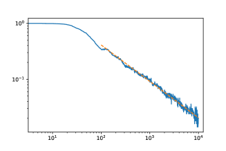
We conjecture that the Betti numbers of finite preferential attachment clique complexes with nodes admit a scaling limit, in the sense that the mean-normalized Betti numbers converge in distribution as . The right panel of Figure 1 shows the evolution of the complementary cumulative distribution functions () of the mean-normalized Betti numbers. Visually, the nearby curves suggest the distributions converge. Further details about this simulation, including model parameters and Kolmogorov-Smirnov statistics, will be detailed in Section 9 to support the conjectural convergence. The curves in the right panel of Figure 1 are visually pretty straight, and the fitted slope of the limiting distribution is , which means the power-law distribution has a finite variance. We note that this exponent depends on the model parameters, and it is not necessarily larger than . More simulation results for other model parameters than the ones for the right panel of Figure 1 will be presented in Section 9. Codes for our simulations are available at The GitHub repo carolinerongyi/Preferential_Attachment_Clique_Complex.
1.3 Intuition for our Homotopy-Connectedness Result
It was observed in [Siu et al., 2023] that the growth in Betti numbers in preferential attachment clique complexes is driven by the formation of (not necessarily disjoint) small spheres, and these spheres become boundaries at a much slower rate than their formation. Shmuel Weinberger conjectured that, since all such spheres should eventually become boundaries of balls, the infinite complexes, where the rate is no longer relevant, may be contractible. Our result formally verifies that such spheres are indeed the main obstruction to homotopy-connectedness. The infinite complexes are, however, not contractible, because the restriction on the number of edges implies certain cycles can never become boundaries.
1.4 The Subtlety of the Limiting Topology
The above intuition also explains the apparent paradox that Betti numbers of the finite complexes, by Theorem 4.1, diverge to infinity, while the infinite complexes, by Theorem 4.2, are homotopy-connected (and hence their Betti numbers vanish). For readers who are interested in persistent homology (Cf. Chapter VII.1 of [Edelsbrunner and Harer, 2010]), this discrepancy may be seen as a consequence of the facts that the persistence diagrams of preferential attachment clique complexes, filtered by node arrival, have infinitely many points with high probability, but almost surely none of them has an infinite death time.
This subtlety, however, does highlight the difficulty of studying the scaling limits of topological properties of random models. Topological operations may not commute with analytical limits, in the sense that a topological property of an analytically defined limiting object of a random model is not necessarily the same as the analytical limit of the corresponding topological properties of the random model. In symbols, we have
for many topological operations TopOp and many (analytically defined) limiting operations .
There are two main sources of noncommutativity:
- The Global Nature of Topology
-
Since topological properties are often global in nature, locally defined analytical limits may fail to capture these properties.
- Small Support of Nontrivial Topological Behavior
-
Many analytical limiting operations involve some kind of rescaling, e.g. the central limit theorem states that, upon scaling by , converges in distribution to a normal distribution under mild assumptions. In particular, variations vanish in the limit upon rescaling. If the nontrivial topological behavior is supported on a very small part of the spaces concerned, it may vanish upon rescaling when taking an analytical limit.
We illustrate these sources with examples below, but before that, we note that we have been carefully qualifying all instances of “limit” with “analytical”, because some topological operations do commute with limiting procedures in category theory, at least to a certain extent. For example, the theorem in Chapter 14.6 of [May, 1999] states that, under mild conditions, the homology groups of the colimit of a sequence of nested spaces are the colimit of their homology groups. However, for many random models, the underlying category is unclear, and so are the relevant morphims between different terms in the sequence. Even when these are clear, the categorical limit and the analytical limit may have very different properties.
Now, we give examples to illustrate the two sources of noncommutativity above, as well as the discrepancy between analytical and categorical limits.
In the first three examples below, we consider the Benjamini-Schramm limit for random graphs [Benjamini and Schramm, 2001, Aldous and Steele, 2004]. This limit is local in nature in the sense that it is determined by the behavior of metric balls.
Example 1.3 (Increasingly Large Cycles).
To illustrate the first source of discrepancy above, consider the family of 2-regular and connected graphs. Let be, deterministically, the cycle graph with nodes, e.g. is the octagon. Let be deterministically the linear graph with countably infinitely many nodes. Then is the Benjamini-Schramm limit of (Cf. Figure 10 of [Agostini, 2021]).
Now, each has (in fact, is) a cycle. Topologically, the 1-dimensional Betti number of each is 1. However, has no cycle, and the 1-dimensional Betti number is . Therefore, the 1-dimensional Betti number (the topological property) of the Benjamini-Schramm limit (the analytical limit) of is different from the numerical limit (the analytical limit) of the 1-dimensional Betti numbers (the topological property) of ’s.
The limit fails to capture the loops in the ’s because the limit is local in nature, while the loops in the ’s become bigger and bigger and they are eventually not contained in any metric balls of finite radii.
Example 1.4 (Preferential Attachment Graphs).
To illustrate the second source of discrepancy above, note that the Benjamini-Schramm limit of preferential attachment graphs is a random tree (Cf. Theorem 1.5 of [Garavaglia et al., 2023])
All the algebraic-topological properties of a (random) tree are trivial. In particular, the Betti numbers (the topological property) of the Benjamini-Schramm limit (the analytical limit) of preferential attachment clique complexes, are zero at all positive dimensions almost surely.
On the other hand, our results and those in [Siu et al., 2023] show that preferential attachment graphs have non-trivial limiting topological properties. By Theorem 3 of [Siu et al., 2023], the numerical limits of the expectation (the analytical limit) of the Betti numbers (the topological property) of preferential attachment graphs are infinite, say at dimension 2, for some choices of parameters.
This discrepancy can be explained as follows. The Benjamini-Schramm limit of preferential attachment graphs is a tree because most metric balls in preferential attachment graphs are trees. While these graphs do have nontrivial topological behavior (in terms of Betti numbers), such behavior is supported on a small portion of nodes, namely, the ’s in the subsection titled “Dominating Cycles and Proof Synopsis” of Section 1 of [Siu et al., 2023]. Therefore, when one takes the Benjamini-Schramm limit by averaging over all nodes, since there are not too many such ’s, their effect gets washed out in the limit.
Example 1.5 (Subtleties of Categorical Limits).
Our homotopy-connectedness result, Theorem 4.3, illustrates the discrepancy between analytical and categorical limits, as well as the subtlety of categorical limits.
First, as the categorical colimit of the finite complexes, the infinite complex has infinite Betti numbers almost surely for some parameters, whereas the Betti numbers of the Benjamini-Schramm limit, a random tree, vanish almost surely except at dimension 0.
Second, even though the homology groups of the infinite complex are the colimit of the homology groups of the finite complexes, this does not mean that the Betti numbers, which are the ranks (or dimensions) of the homology groups, of the infinite complexes are the limits of those of the finite complexes, as we have noted at the beginning of this subsection. This is because the colimit takes into account the inclusion maps between different finite complexes, and this information is lost when one takes the numerical limit of Betti numbers.
The noncommutativity and discrepancy are not peculiar to the Benjamini-Schramm limit. Consider, for instance, the Eden model, a model for simulating cell division [Eden, 1961, Auffinger et al., 2017]:
Example 1.6 (Eden Model).
A cell in is a volume-1 hypercube whose vertices are in . The Eden cluster in is the stochastic process of subsets of defined as follows.
-
•
is deterministically the cell in the positive octant that contains the origin.
-
•
is the union of and a uniformly randomly chosen cell that is outside of and shares at least a face with at least a cell in .
For the Eden model, the limiting cluster is convex [Cox and Durrett, 1981], and hence has trivial topology, while the Betti numbers of the cluster diverge to infinity with high probability [Manin et al., 2023]. The second source of discrepancy applies in this case, as all nontrivial topological behavior is supported on a thin collar near the boundary of the limiting convex set.
With these examples in mind, one must exercise caution when discussing the limiting behavior of topological properties.
1.5 Paper Outline
The rest of the paper is organized as follows. First, we further contextualize our work in the literature in Section 2. Then, we state our setup in Section 3 and the main results in Section 4. We prepare for the proofs of the main results by recalling relevant results from the literature in Section 5. We begin proving the main results in Section 6 by giving a synopsis of our proofs, and establishing two intermediate results. We finish the proofs in Section 7. We collect more technical proofs of intermediate results in Section 8. We discuss our simulations in Section 9 and future directions in Section 10. We collect background materials in algebraic topology in the appendices. We discuss homology and homotopy theory in Appendices A and B. We discuss the difficulty of homotopy theory at the end of Appendix B, and we contrast the two in Appendix C.
1.6 Acknowledgements
This research was partially funded by the AFOSR grant FA9550-22-1-0091.
This research was partially supported by the Cornell University Center for Advanced Computing, which receives funding from Cornell University, the National Science Foundation, and members of its Partner Program.
The author would like to thank Gennady Samorodnitsky for valuable discussions and feedbacks on the proofs of the main results and on the manuscript; and Shmuel Weinberger for suggesting the question. He also thanks Avhan Misra for assistance with simulations. He thanks Jason Manning, Henry Adams, Lorenzo Ruffoni, and Benjamin Thompson for insightful discussion.
2 Literature Review
This work builds on two strands of research, namely the study of higher-order connectivity of scale-free networks, and the study of random simplicial complexes.
Connectivity of scale-free networks has been widely studied. The clustering coefficients of various models were investigated in [Bollobás and Riordan, 2002, Holme and Kim, 2002, Eggemann and Noble, 2011, Ostroumova et al., 2013, Ostroumova Prokhorenkova, 2017]. In [Garavaglia and Stegehuis, 2019], the growth rate of the expected number of small motifs in preferential attachment graphs was determined. In [Bianconi and Rahmede, 2016, Courtney and Bianconi, 2017], some forms of higher-dimensional degrees were considered in some forms of preferential attachment simplicial complexes.
Algebraic-topological properties of scale-free networks are much less studied. The 1-dimensional Betti number of a scale-free simplicial complex was considered in [Oh et al., 2021]. The asymptotics of the expected Betti numbers of all dimensions of preferential attachment clique complexes were established in [Siu et al., 2023]. The central limit theorem for the Betti numbers of the age-dependent random connection clique complexes was established in [Hirsch and Juhasz, 2023] in the light-tailed regime. To our knowledge, these are the only analytical results about algebraic-topological properties of random scale-free networks in the literature. The current work is largely an extension of [Siu et al., 2023]. Phase transitions of the Euler characteristic of preferential attachment graphs were numerically observed in [de Amorim Filho et al., 2022], where the Euler characteristic is defined in terms of the sum of discrete curvature as opposed to Betti numbers.
On the other hand, there has been a growing literature on random simplicial complexes and their algebraic-topological properties. We refer the reader to [Kahle et al., 2014, Bobrowski and Krioukov, 2022] for comprehensive surveys. Below, we highlight results on homotopy-connectedness and phase transitions. As mentioned in Section 1.2, many random simplicial complexes exhibit two phase transitions for each dimension. In some situations, it can also be shown that at some point after the second transition, the complex becomes homotopy-connected. This is the case for the Erdos-Renyi clique complex [Kahle, 2014], with a homotopy-connectedness result in [Kahle, 2009]; and random Cech and Rips complexes [Kahle, 2011, Kahle and Meckes, 2013, Yogeshwaran and Adler, 2015]. For the Linial-Meshulam models, since they have maximal simplices (simplices that are not faces of other simplices) in only two adjacent dimensions, there is only one phase transition at the lower dimension [Linial and Meshulam, 2006, Meshulam and Wallach, 2009, Kahle and Pittel, 2016].
For percolation models, phase transition is often defined in terms of the emergence of giant cycles as opposed to the surge in the number of cycles. Typically, there is a threshold at which giant cycles of the underlying manifold appear, possibly simultaneously at the threshold [Bobrowski and Skraba, 2020, Duncan et al., 2023]. Defined slightly differently, the phase transition of the emergence of the giant component in the graph of holes was studied in [Hiraoka and Mikami, 2020].
3 Setup
We first define the preferential attachment model, which was first proposed in [Barabási and Albert, 1999]. Our notations follow those in [Siu et al., 2023].
Definition 3.1 (Affine Preferential Attachment Graphs; Definition 4.3.1 of [Garavaglia, 2019]).
Let and be positive integers with and let . The preferential attachment graph is the random graph, with no self-loops but possibly with repeated edges, that is constructed inductively as follows.
-
•
is the deterministic graph with two nodes, indexed by 1 and 2, and edges from node 2 to node 1.
-
•
is constructed by adding a node, indexed by , to and edges from node to randomly chosen nodes in one by one from the following conditional distribution:
for , where is the graph after adding edges from to , and the normalization constant is .
-
•
.
Remark.
To the best of our knowledge, the case for but with a general was first considered in [Móri, 2002]. The definition above is equivalent to the model in Definition 4.3.1 of [Garavaglia, 2019] and defined by (1.3.65) of [van der Hofstad, 2024a], modulo typos in the latter [van der Hofstad, 2024b]. For lists of other variants of the preferential attachment model, see [Ostroumova Prokhorenkova, 2017] and Chapter 4.3 of [Garavaglia, 2019].
Throughout this paper,
| (1) |
and our main results will be stated in terms of .
Remark.
We make two remarks on notations.
-
•
Sometimes we may drop the arguments and write to simplify notation.
-
•
Despite the convention in the literature of preferential attachment graphs, we refrain from denoting this quantity by to avoid confusion with the Euler characteristic, a topological invariant.
This quantity increases with and it can be seen as an alternative measure of the strength of preferential attachment. It is related to the rate at which the probability of forming an edge between a new node and an early node converges to . More precisely, we have the following proposition. (See also Exercise 8.13 and Lemma 8.17 of [van der Hofstad, 2016] for an analogous theorem about a slightly different preferential attachment model.)
Proposition 3.2.
Let be positive integers. Let be the probability that node is attached to node in the preferential attachment graph via at least one edge. Then there exist positive constants such that
Proof.
We merely sketch the proof because we will not use this proposition in the rest of the paper. For the lower bound, apply Lemma 1 of [Garavaglia and Stegehuis, 2019] with , , and . For the upper bound, sum over the upper bounds given by the lemma for the same choices of , but all possible choices of , namely . Note that the lemma has a typo: nodes in should precede those in . ∎
We conclude this section by defining preferential attachment clique complexes. We recall algebraic-topological notions like simplicial complexes in Appendix A.
Definition 3.3 (Preferential Attachment Clique Complexes).
Let be a positive integer and . For , the preferential attachment clique complex is the simplicial complex with the same nodes as , and is a simplex in if and only if there is at least one edge between each pair of distinct nodes in .
4 Main Results
Before we state our results, we remark on some probabilistic terminologies and conventions.
-
•
A property is said to hold almost surely if it holds with probability 1.
-
•
A property is said to hold asymptotically almost surely if the probability that it holds converges to 1.
-
•
Throughout this paper, and denote generic constants which may change from line to line or within the same line, unless when they are explicitly stated to be specific constants (the only such exception is in the definition of right after Equation 2). Their subscripts denote variables on which they may depend.
Our first main result concerns the scaling limit of the Betti numbers.
Theorem 4.1.
Let be the Betti number of at dimension . Suppose , , , and . Then the following inequalities hold asymptotically almost surely.
Our second main result concerns the homotopy-connectedness of :
Theorem 4.2.
If , and , then is -homotopy-connected almost surely.
In particular, all Betti numbers of vanish up to dimension , inclusively.
Our third main result addresses the tightness of the condition in the previous theorem.
Theorem 4.3.
Suppose and and . Then the Betti number of , in field coefficients, is almost surely infinite if ; it is almost surely finite if and .
Remark.
See Definition A.4 for the definition of homology with coefficients.
Indeed, if the Betti number in rational coefficients is infinite, then by Corollary 3A.6a of [Hatcher, 2002] (Proposition A.5), the homology group (in integer coefficients) cannot vanish, and hence the space cannot be -homotopy-connected by Hurewicz’s theorem (Theorem B.6).
5 Preliminaries
In this section, we state the preliminary facts on which the proofs of our main results are based. Topological facts are collected in the appendices.
5.1 An Equivalent Formulation of Finite Preferential Attachment Graphs
The Polya urn’s interpretation of the preferential attachment graph affords an equivalent formulation of the random graph process, which is sometimes more amenable to analytical computations.
Definition 5.1 (Finite Polya Preferential Attachment Graphs).
Let be a positive integer and . Let be a positive integer. The finite Polya preferential attachment graph is defined as follows.
-
•
Let be independent random variables with and .
-
•
Let
-
•
Let , where and , be an array of conditionally independent random variables given , and . Let be the unique index such that .
-
•
consists of nodes, indexed by , and one edge from node to node for each and .
Theorem 5.2 (Theorem 4.4.3 of [Garavaglia, 2019]).
If is finite, then and have the same distribution.
Remark.
Since the two graphs have the same distribution, we drop the subscript “Polya” hereafter.
The ’s decouple the dependency of different edges:
Lemma 5.3.
Given , all edges are conditionally independent, and the conditional probability that a node is connected to a node via its edge is , which is independent of .
Proof.
Direct verification, see also (5.3.32) and (5.3.33) of [van der Hofstad, 2024a]. ∎
We have the following variant of Proposition 5.18 of [van der Hofstad, 2024a] and Lemma 3.1 of [Berger et al., 2014] regarding the asymptotics of ’s.
Proposition 5.4.
There exists a positive constant such that for every and, every positive integer , with probability at least it holds that
and hence there exist positive constants such that for all ,
Proof.
Postponed to Section 8. ∎
5.2 Homology of Finite Preferential Attachment Clique Complexes
We set up for the results from [Siu et al., 2023] as follows.
-
•
Let be a clique complex with vertices .
-
•
Let be the link of in . We recall the definition of link in Definition A.3.
-
•
Let be the subcomplex of consisting of all simplices of whose vertices are in .
-
•
For a subcomplex of , a nonnegative integer , nodes of such that and all nodes in strictly precede , let
-
–
be the event where is isomorphic to the -dimensional octahedral sphere (with the simplicial complex structure of the -unit sphere in , see the second bullet point of Remark Remark for a formal definition of ) and all nodes in are connected to both and , and
-
–
,
where denotes the indicator function of the event . The quantity is the relative Betti number. Its precise definition, which can be found in Section 9 of [Munkres, 1984], needs not concern us here, as the results below give us all information we need about this quantity.
-
–
We need the following results.
Proposition 5.5 (Proposition 14 of [Siu et al., 2023]).
Let be a clique complex with vertices labeled by positive integers. Let , be a subcomplex of , and be a node that is strictly preceded by all nodes in . Then
Proposition 5.6 (Lemmas 19 and 20 of [Siu et al., 2023]).
Let . Suppose . Let . Let be a (possibly random) subcomplex of , and be a (possibly random) node in that is (almost surely) strictly preceded by all nodes in . Then
whenever the exponents of are positive. For each inequality, if the exponent is zero or negative, the bound still holds when the expression in is replaced by or respectively.
5.3 A Criterion for Homotopy-Connectedness
We need the following criterion for homotopy-connectedness.
Theorem 5.7 (Barmak; Theorem 4 in the appendix of [Farber, 2023]).
Let be a nonnegative integer and be a simplicial complex. If every subcomplex with at most vertices is contained in the star of a vertex , then is -homotopy-connected.
6 Proof Synopsis and Two Intermediate Results
In this section, we sketch our proof and establish two intermediate results (and their corollaries), from which the main results will follow without much complication.
Regarding Theorem 4.1 for , since the first moments of the Betti numbers have been estimated in [Siu et al., 2023], the upper bounds follow directly from Markov’s inequality. For the lower bounds, in light of Proposition 5.5, it suffices to establish a concentration result for the number of common neighbors of a finite set of nodes (namely nodes in ). This is the content of Proposition 6.1 below. Of course, to satisfy the assumptions of Proposition 5.5, this finite set of nodes has to form a sphere, so we also need a result on the existence of spheres in preferential attachment complexes. This is the content of Proposition 6.3 below.
It turns out the aforementioned concentration result also allows us to apply Theorem 5.7 to establish Theorem 4.2.
As in [Siu et al., 2023], the proof of Theorem 4.1 for is based on Morse theory.
Finally, given the preliminary facts, Theorem 4.3 is a straight-forward corollary of the other results.
We now state the intermediate results we need.
Proposition 6.1.
Suppose and . Fix nodes in the infinite preferential attachment graph . Let be the indicator of the event where node is a common neighbor of . Then for every there exists a constant such that with probability at least , for ,
We prove this proposition at the end of this section.
Corollary 6.2.
Suppose . If , then every collection of distinct nodes has infinitely many common neighbors in the infinite preferential attachment graph almost surely.
Proof.
The above proposition implies that, for every , the probability that the nodes have at most common neighbors in is bounded above by by considering with a sufficiently large . Hence the said probability is in fact . The result follows by taking union with ranging over all positive integers. ∎
Remark.
Putting shows that the diameter of the infinite preferential attachment graph is 2 almost surely. Geodesics between disconnected nodes go through nodes in the distant future. This behavior is markedly different from that of finite preferential attachment graphs, where short paths tend to pass through nodes in a small core of nodes [Dommers et al., 2010].
Proposition 6.3.
If and , then contains an as an induced subgraph almost surely, where denotes the graph formed by replacing repeated edges by single edges.
Proof.
We prove the proposition by induction. The case for is trivial, as is just two disconnected points. Inductively, assume contains an as an induced subgraph. By Corollary 6.2, the nodes of this have infinitely many common neighbors, and they cannot all be connected with each other (since the common neighbor cannot be connected with all previous ones). Then contains, as an induced subgraph, an that contains the above as the equator and two disconnected common neighbors of the nodes of the as the poles. ∎
Corollary 6.4.
If and , then for every , for , with probability at least , contains an as an induced subgraph.
Proof.
For , let be the event that contains an as an induced subgraph. Then
∎
Before proving Proposition 6.1, we first establish a lemma.
Lemma 6.5.
Consider the Polya urn model (Cf. Definitions 5.1 and 5.2). Suppose . Let be the conditional probability that given . Then for ,
Proof.
The second inequality follows directly from the first one, because . For the first inquality, we use the two-term Bonferroni inequality (Exercise 1.6.10 of [Durrett, 2019]):
For distinct integers , let be the event where the is connected to via ’s edge, for .
Then is the union of the ’s. There are distinct choices of .
By Lemma 5.3,
| If , then | ||||
where the last inequality holds because implies , and each , being a probability, lies in . The lemma then follows by applying the two-term Bonferroni inequality. ∎
Proof of Proposition 6.1.
Fix . We consider the Polya urn model (Cf. Definitions 5.1 and 5.2) and condition on . Then ’s are conditionally independent Bernoulli random variables.
By Proposition 5.4, there exist positive constants such that the event defined by
has probability at least .
Let be the event where , where is chosen such that is at most . This is possible by the continuity of Beta distributions.
Recall that Lemma 6.5 gives the lower bound of , the conditional probability that given . On , which is -measurable, if for some , the parenthesized factor (not the binomial coefficients) in the last line of Lemma 6.5 is at least and hence
because depends on and for every .
The Chernoff bound then implies that, on , for every ,
| (2) |
where all sums here range over . Picking and to be times the specific in Equation 2 gives
for some generic positive constant . The divergence of implies that the right-hand side is less than for large enough .
Therefore, by the -measurability of ,
The proposition then follows by noting that has the desired order of magnitude. ∎
7 Proofs of Main Results
Proof of Theorem 4.2.
Apply Corollary 6.2 with Theorem 5.7. ∎
Proof of Theorem 4.1 for .
We only prove the case for . The case for is analogous.
Similarly, in the notations of Proposition 5.6 and Proposition 5.5, it holds asymptotically almost surely that
regardless of the choice of and (as longs as the ’s are well-defined).
Let be the random subcomplex in that is the first subcomplex isomorphic to as an induced subcomplex. If such a subcomplex does not exist, let be the induced subcomplex on the first nodes. (This choice will be immaterial.)
Let be the random first node after those in that is connected to all nodes in . If such an does not exist, let be the first node after those in .
It suffices to bound
Fix . By Corollary 6.4, for large enough, .
By Proposition 6.1, conditioning on shows that for large enough,
The result then follows.
∎
Proof of Theorem 4.1 for .
We follow the proof of Proposition 4 of [Siu et al., 2023]. Let , , and be the (multi-)sets of vertices, edges and triangles of . Let and be the set of edges and triangles of . The strong Morse inequality (Theorem 1.8 of [Forman, 2002]) implies that
where denotes cardinality. Let be the number of “biangles” in (two-node subgraphs with two (repeated) edges between them). Since and ,
The rest of the proof follows from Markov’s inequality and Theorem 1 of [Garavaglia and Stegehuis, 2019].
∎
Before we prove Theorem 4.3, we need a lemma to compute the homology groups of the union of a nested sequence of spaces.
Lemma 7.1.
Let . Let be a nested sequence of simplicial complexes. Suppose the inclusion maps induce injective homomorphisms on eventually (induced homomorphism defined in Definition A.6). Then
Proof.
Deferred to the end of Section 8. ∎
Proof of Theorem 4.3.
In order to invoke Lemma 7.1 to reduce the computation to one for finite complexes, we show that the inclusion map induces an injective homomorphism between
eventually. Indeed, since , for the relevant sum in Proposition 5.6 to converge to a finite number almost surely, must be eventually almost surely, and hence, with field coefficients must vanish (Cf. the second bullet point after Definition A.4). The segment of the Mayer-Vietoris sequence (Theorem A.7) of
then implies that the latter map is eventually injective almost surely.
Now, Lemma 7.1 shows it suffices to show almost surely, or is bounded almost surely, depending on whether . For the former case, since is eventually increasing, it suffices to show that for every and every , with probability at least , eventually. This is a simple consequence of Theorem 4.1. The first case then follows. The other case follows from putting in the first estimate of Proposition 5.6 into Proposition 5.5 and applying Markov’s inequality.
∎
8 Proofs of Preliminary Facts
Proof of Proposition 5.4.
We largely follow the proof of Lemma 3.1 of [Berger et al., 2014]. Since , consider the approximation
where all sums above range over , the same for sums with unspecified ranges hereafter.
The first term, which is the only random term, forms a martingale when varies (and is fixed). Kolmogorov’s inequality (Theorem 2.5.5 of [Durrett, 2019]) gives
| (3) |
where is to be chosen. Since for , for ,
where denotes the Beta function. Therefore, the right-hand side of Equation 3 is bounded from above by if .
For the second term, since for ,
where, again, the the far-left term is bounded below by .
For the last term,
because .
The result then follows. ∎
Proof of Lemma 7.1.
This is a special case of the theorem in Chapter 14.6 of [May, 1999], which states that under assumptions more general than ours, the homology group of the union is the colimit of the homology groups. In the remainder of the proof, we do the routine checking that the group on the right-hand side is indeed the colimit, which is defined in Chapter 2.6 of [May, 1999].
Denote by the homomorphism induced by the inclusion . By assumption, there exists some such that is injective for . Denote by the union of groups in the lemma, where “large enough” means . Let be the inclusion homomorphism for . For , define .
To check that is indeed the colimit, it suffices to show that for every abelian group and every sequence of homomorphisms , if for every , then there exists a unique homomorphism such that
| (4) |
Fix and the ’s. Define as follows. For each , for some and . Define , which is equivalent to Equation 4. Therefore, if is well-defined, then is the desired map and it is unique. To see that is well-defined, note that once is chosen, is uniquely determined because is injective for . The choice of is immaterial because if for some , then (by the injectivity of ) and hence (by the assumption on the ’s).
To see that is a homomorphism, fix and with . Suppose . Let , hence . Hence
∎
9 Simulations
In this section, we present further numerical evidence that the mean-normalized Betti numbers of finite preferential attachment clique complexes have limiting distributions that obey power laws.
We first provide further details about the right panel of Figure 1 in the Introduction. We simulated 500 complexes with 10000 nodes and with parameters and and observe the evolution, as the number of nodes increases, of the distribution of the mean-normalized Betti number at dimension 2, where is the sample mean of the Betti numbers at dimension 2.
The left panel of Figure 3 shows the log-log plot of the evolution of the Kolmogorov-Smirnov norm between the distributions of normalized Betti numbers at time and time . It is estimated that the norm converges to 0 at a rate of .
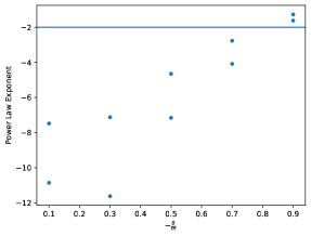
We now vary the model parameters and and we increase the number of trials to . We approximate the limiting distribution by the one for the complex with nodes. This simulation was done by Avhan Misra. The right panel of Figure 3, prepared by Misra, shows the fitted exponents. We note that the fitted exponents on the far right for are less negative than . Therefore, the limiting distribution, if existent, may have an infinite variance. We also note that the right-hand side of the figure also shows that the fitted exponent is not a function of , even though all our theoretical results depend on and through only.
10 Future Directions
Building on [Siu et al., 2023], we have established the asymptotic almost sure limits of the orders of magnitude of the Betti numbers of finite preferential attachment clique complexes, and we have established phase transitions for the infinite complexes for each dimension. Open questions about the algebraic-topological properties of preferential attachment complexes abound.
First, numerical evidence suggests the Betti numbers admit a scaling limit. Considerable effort is likely necessary to combine homological algebra and analysis to prove this conjecture. In fact, even the moments of the Betti numbers are not well understood.
Second, as discussed in the Introduction, common notions of analytical limits do not necessarily preserve topological properties. In order to study the large-scale topological behavior of random models, a suitable notion of convergence is yet to be developed.
Third, the topology of other related random models are yet to be studied. Our argument relies heavily on the alternative description of our specific preferential attachment model in Definition 5.1. It remains to be seen whether the topological behavior of this model is universal across different modes of preferential attachment. Further, since many real-world networks have different clustering behavior from preferential attachment models [Ostroumova Prokhorenkova, 2017], much work is needed to study the topological behavior of other random models with more complicated clustering behavior.
Appendix A Homology Theory
Homology groups and Betti numbers are defined in Definition 1.2. Here we fill in gaps in this definition. We follow the exposition in [Munkres, 1984] as far as possible.
First, we define simplicial complexes.
Definition A.1 (Simplicial Complex; Section 3 in Chapter 1 of [Munkres, 1984]).
A simplicial complex with totally ordered vertices is a collection of finite nonempty subsets of a totally ordered set that is closed under inclusion , i.e. whenever for some . Elements in this collection are called simplices, and the dimension of a simplex is one less the number of elements in this simplex (as a subset of the totally ordered set). - and -dimensional simplices are called vertices and edges.
Remark.
-
•
Simplicial complexes thus defined are often called abstract simplicial complexes, to distinguish them from their geometric realizations, which are unions of geometric simplices in Euclidean spaces. We only consider abstract simplicial complexes in this paper, with the only exception of the sphere in the bullet point in Section 5.2. There, we define as the unit sphere, which is a union of geometric simplices in . Throughout this paper, we think of as the abstract simplicial complexes whose geometric realization is such a union. Alternatively, may be defined as the clique complex (defined in Definition A.2) with vertices where and are connected by an edge if and only if .
-
•
Section 3 of [Munkres, 1984] starts with the discussion on oriented simplices. We do not need such notion for Definition 1.2 because we specialize to the case when the vertices are totally ordered. Indeed, there is a natural orientation on each simplex, namely the monotone ordering.
Definition A.2 (Clique Complex).
A simplicial complex is said to be a clique complex if for distinct vertices , is a simplex whenever there is an edge between every pair of distinct and .
The link of a vertex in a simplicial complex is defined as follows.
Definition A.3 (Star and Link; p.11 of [Munkres, 1984]).
-
•
The star of a vertex in is the subcomplex of consisting of all simplices containing (and the faces of these simplices).
-
•
The link of a vertex in is the subcomplex of the star of that consists of all simplices that do not contain .
Remark.
Our notion of star is called the closed star in [Munkres, 1984].
Next, we address the choice of coefficients.
Definition A.4 (Homology with Arbitrary Coefficients; Section 51 of [Munkres, 1984]).
Let be a simplicial complex with totally ordered vertices and be an abelian group. Let and be the chain groups and boundary maps in Definition 1.2. Let .
The homology group at dimension with coefficients in is defined by , where denotes the identity on .
See Section 10 in Chapter 1 of [Munkres, 1984] for a less intimidating but more verbose definition.
-
•
If , one recovers Definition 1.2.
-
•
If is a field, then the homology groups are vector spaces, and hence they vanish if and only if their Betti numbers vanish.
-
•
We often denote by if the choice of coefficients is implied.
Proposition A.5 (Homology with Rational Coefficients; Corollary 3A.6a of [Hatcher, 2002]).
Let be a topological space. Then
Finally, we define induced maps between homology groups. A simplicial map between two simplicial complexes is a function between the vertex sets of the two complexes such that is a simplex in for every simplex .
Definition A.6 (Induced Maps Between Homology Groups; Section 2 of Chapter 1 of [Munkres, 1984]).
For every integer , every simplicial map induces a homomorphism defined by
where is the permutation on such that is monotonically increasing under the ordering of vertices of . This map in turn induces a homomorphism defined by
for every -cycle of , where the two superscripted ’s are the boundary groups of and respectively.
Theorem A.7 (Mayer-Vietoris Sequence; Theorem 25.1 of [Munkres, 1984]).
Let and be subcomplexes of a simplicial complex . Then there exist maps such that the following sequence is exact.
A sequence is said to be exact if for every . (Cf. Section 23 of [Munkres, 1984]) In particular, if , then is injective.
Appendix B Homotopy Theory
Homotopy and homotopy-connectedness are defined in Definition 1.1. We start by filling gaps in the definition. We follow the exposition in Chapters 0 and 4 of [Hatcher, 2002]. For applications of the concept of homotopy-connectedness in graph theory, see Sections 4 and 6 of [Björner, 1996].
Homotopy-connectedness is typically defined via homotopy groups, whose elements are, intuitively speaking, spherical “holes” of the space.
Definition B.1 (Homotopy Groups; p.340 – 341 of [Hatcher, 2002]).
Let be a nonnegative integer and be the -dimensional sphere. Fix . Let be a topological space and .
As a set, the homotopy group of with base-point at dimension is the set of equivalence classes of maps such that , where the equivalence relation is homotopy. In symbols
if and only if and are homotopic.
Remark.
-
•
Homotopy groups, as their names suggest, are groups, but we will not describe the group operation because we never use it in this paper.
-
•
Two equivalent definitions of homotopy groups are given in [Hatcher, 2002]. The version above is stated at the last paragraph of p.340.
-
•
We note that if is path-connected, then and are isomorphic for every .
Example B.2.
For spheres, , and for . This is a testimony to the facts that a sphere has a spherical hole of its dimension, and that it has no lower-dimensional hole.
Definition B.3 (Homotopy-Connectedness; p.346 of [Hatcher, 2002]).
A space is said to be -homotopy-connected if and only if for every and every .
Remark.
-
•
In [Hatcher, 2002], -homotopy-connectedness is abbreviated to -connectedness. We refrain using from this abbreviation to avoid confusion with another graph-theoretic concept, which describes graphs that remain connected after the removal of vertices.
-
•
One may readily verify that Definition 1.1 and this definition are equivalent.
Intuitively, in a 1-homotopy-connected space, also known as a simply-connected space, every pair of paths are connected by a path of paths; in a 2-homotopy-connected space, every pair of paths of paths are connected by a path of paths of paths, etc, because the image of the two hemispheres of can be viewed as the pair of paths of paths and the image of the 3-dimensional ball as the path of paths of paths.
Definition B.4 (Contractible; p.4 of [Hatcher, 2002]).
A space is said to be contractible if the identity map on is homotopic to a constant map.
Theorem B.5 (Whitehead’s Theorem; Theorem 4.5 of [Hatcher, 2002]).
Let be a map between two connected CW complexes and let . If is an isomorphism for every positive integer , then is a homotopy equivalence, i.e. there exists a map such that , and and are homotopic to the identity maps on and respectively.
Remark.
As a corollary, if is path-connected and for every positive integer , then letting be the inclusion of in shows is contractible. (See the second paragraph of p.348 of [Hatcher, 2002].)
Theorem B.6 (Hurewicz’s Theorem; Theorem 4.32 of [Hatcher, 2002]).
If a space is -homotopy-connected for some integer , then for and for every .
We conclude this section by commenting on the difficulty of homotopy theory and sampling some positive results. The difficulty of homotopy theory is best illustrated by the fact that the computation of the higher homotopy groups of spheres is still an active area of research. In fact, even the computation of the higher stable homotopy groups of spheres, which are better behaved than higher homotopy groups, is difficult.
However, the ranks of the higher homotopy groups of spheres are known (Cf. Serre’s finiteness theorem, viz. Proposition V.3.3 and Corollary V.6.2 of [Serre, 1951]): if ,
For another positive result regarding the computation of homotopy groups, for each fixed , there is a polynomial-time algorithm to compute for simplicial complexes such that [Čadek et al., 2014].
Appendix C Comparison between Homology and Homotopy Groups
Homology groups and homotopy groups both capture holes of spaces, but they are subtly different. Homology is more flexible about both holes and trivial holes, in the sense that every map on a sphere gives rise to a cycle, while every path between maps on spheres also gives rise to a boundary. The converse is not true for each case. Consider, for instance, the torus. Its homology group at dimension 2 is , which is generated by the torus itself as a cycle. The homotopy group at dimension 2, however, is trivial. In this case, homology captures more structures. On the other hand, consider the torus with a small disc removed. The boundary of the small disc is a nontrivial element in the 1-dimensional homotopy group (it is , where and are the longitude and the meridian of the torus), but it is a trivial element in the homology group, because it is the boundary of the whole space as a 2-cycle.
References
- Agostini [2021] G. S. Agostini. Benjamini-Schramm convergence of random rooted graphs, 2021. URL https://www.uvm.edu/~smillere/TProjects/GAgostini21f.pdf.
- Aldous and Steele [2004] D. Aldous and J. M. Steele. The Objective Method: Probabilistic Combinatorial Optimization and Local Weak Convergence, pages 1–72. Springer Berlin Heidelberg, Berlin, Heidelberg, 2004. ISBN 978-3-662-09444-0. doi: 10.1007/978-3-662-09444-0˙1. URL https://doi.org/10.1007/978-3-662-09444-0_1.
- Auffinger et al. [2017] A. Auffinger, M. Damron, and J. Hanson. 50 Years of First-Passage Percolation. University Lecture Series. American Mathematical Society, 2017. ISBN 9781470441838. URL https://www.ams.org/books/ulect/068/.
- Barabási and Albert [1999] A.-L. Barabási and R. Albert. Emergence of scaling in random networks. Science, 286(5439):509–512, 1999. doi: 10.1126/science.286.5439.509. URL https://www.science.org/doi/abs/10.1126/science.286.5439.509.
- Battiston et al. [2020] F. Battiston, G. Cencetti, I. Iacopini, V. Latora, M. Lucas, A. Patania, J.-G. Young, and G. Petri. Networks beyond pairwise interactions: Structure and dynamics. Physics Reports, 874:1–92, 2020. ISSN 0370-1573. doi: https://doi.org/10.1016/j.physrep.2020.05.004. URL https://www.sciencedirect.com/science/article/pii/S0370157320302489. Networks beyond pairwise interactions: Structure and dynamics.
- Benjamini and Schramm [2001] I. Benjamini and O. Schramm. Recurrence of Distributional Limits of Finite Planar Graphs. Electronic Journal of Probability, 6(none):1 – 13, 2001. doi: 10.1214/EJP.v6-96. URL https://doi.org/10.1214/EJP.v6-96.
- Benson et al. [2016] A. R. Benson, D. F. Gleich, and J. Leskovec. Higher-order organization of complex networks. Science, 353(6295):163–166, 2016. doi: 10.1126/science.aad9029. URL https://www.science.org/doi/abs/10.1126/science.aad9029.
- Berger et al. [2014] N. Berger, C. Borgs, J. T. Chayes, and A. Saberi. Asymptotic behavior and distributional limits of preferential attachment graphs. The Annals of Probability, 42(1):1 – 40, 2014. doi: 10.1214/12-AOP755. URL https://doi.org/10.1214/12-AOP755.
- Bianconi [2021] G. Bianconi. Higher-Order Networks. Elements in the Structure and Dynamics of Complex Networks. Cambridge University Press, 2021. doi: 10.1017/9781108770996.
- Bianconi and Rahmede [2016] G. Bianconi and C. Rahmede. Network geometry with flavor: From complexity to quantum geometry. Phys. Rev. E, 93:032315, Mar 2016. doi: 10.1103/PhysRevE.93.032315. URL https://link.aps.org/doi/10.1103/PhysRevE.93.032315.
- Björner [1996] A. Björner. Topological Methods, pages 1819–1872. MIT Press, Cambridge, MA, USA, 1996. ISBN 0262071711.
- Bobrowski and Krioukov [2022] O. Bobrowski and D. Krioukov. Random Simplicial Complexes: Models and Phenomena, pages 59–96. Springer International Publishing, Cham, 2022. ISBN 978-3-030-91374-8. doi: 10.1007/978-3-030-91374-8˙2. URL https://doi.org/10.1007/978-3-030-91374-8_2.
- Bobrowski and Skraba [2020] O. Bobrowski and P. Skraba. Homological Percolation: The Formation of Giant k-Cycles. International Mathematics Research Notices, 2022(8):6186–6213, 12 2020. ISSN 1073-7928. doi: 10.1093/imrn/rnaa305. URL https://doi.org/10.1093/imrn/rnaa305.
- Bollobás and Riordan [2002] B. Bollobás and O. M. Riordan. Mathematical results on scale-free random graphs, chapter 1, pages 1–34. John Wiley & Sons, Ltd, 2002. ISBN 9783527602759. doi: https://doi.org/10.1002/3527602755.ch1. URL https://onlinelibrary.wiley.com/doi/abs/10.1002/3527602755.ch1.
- Courtney and Bianconi [2017] O. T. Courtney and G. Bianconi. Weighted growing simplicial complexes. Phys. Rev. E, 95:062301, Jun 2017. doi: 10.1103/PhysRevE.95.062301. URL https://link.aps.org/doi/10.1103/PhysRevE.95.062301.
- Cox and Durrett [1981] J. T. Cox and R. Durrett. Some Limit Theorems for Percolation Processes with Necessary and Sufficient Conditions. The Annals of Probability, 9(4):583 – 603, 1981. doi: 10.1214/aop/1176994364. URL https://doi.org/10.1214/aop/1176994364.
- de Amorim Filho et al. [2022] E. C. de Amorim Filho, R. A. Moreira, and F. A. N. Santos. The euler characteristic and topological phase transitions in complex systems. Journal of Physics: Complexity, 3(2):025003, may 2022. doi: 10.1088/2632-072X/ac664c. URL https://dx.doi.org/10.1088/2632-072X/ac664c.
- Dommers et al. [2010] S. Dommers, R. van der Hofstad, and G. Hooghiemstra. Diameters in preferential attachment models. Journal of Statistical Physics, 139(1):72–107, 2010. doi: 10.1007/s10955-010-9921-z. URL https://doi.org/10.1007/s10955-010-9921-z.
- Duncan et al. [2023] P. Duncan, M. Kahle, and B. Schweinhart. Homological percolation on a torus: plaquettes and permutohedra, 2023.
- Durrett [2019] R. Durrett. Probability: Theory and Examples. Cambridge Series in Statistical and Probabilistic Mathematics. Cambridge University Press, 5 edition, 2019.
- Edelsbrunner and Harer [2010] H. Edelsbrunner and J. Harer. Computational Topology: An Introduction. Applied Mathematics. American Mathematical Society, Providence, RI, 2010. ISBN 9780821849255. URL https://www.ams.org/books/mbk/069/.
- Eden [1961] M. Eden. A two-dimensional growth process. In J. Neyman, editor, Proceedings of the 4th Berkeley Symposium on Mathematical Statistics and Probability, volume 4, pages 223–239, Berkeley, CA, 1961. University of California Press.
- Eggemann and Noble [2011] N. Eggemann and S. Noble. The clustering coefficient of a scale-free random graph. Discrete Applied Mathematics, 159(10):953–965, 2011. ISSN 0166-218X. doi: https://doi.org/10.1016/j.dam.2011.02.003. URL https://www.sciencedirect.com/science/article/pii/S0166218X1100076X.
- Farber [2023] M. Farber. Large simplicial complexes: universality, randomness, and ampleness. Journal of Applied and Computational Topology, 2023. doi: 10.1007/s41468-023-00134-9. URL https://doi.org/10.1007/s41468-023-00134-9.
- Forman [2002] R. Forman. A user’s guide to discrete morse theory. Séminaire Lotharingien de Combinatoire, 48:B48c–35, 2002.
- Garavaglia [2019] A. Garavaglia. Preferential attachment models for dynamic networks. PhD thesis, Mathematics and Computer Science, Jan. 2019. Proefschrift.
- Garavaglia and Stegehuis [2019] A. Garavaglia and C. Stegehuis. Subgraphs in preferential attachment models. Advances in Applied Probability, 51(3):898–926, 2019. doi: 10.1017/apr.2019.36.
- Garavaglia et al. [2023] A. Garavaglia, R. S. Hazra, R. van der Hofstad, and R. Ray. Universality of the local limit of preferential attachment models, 2023.
- Hatcher [2002] A. Hatcher. Algebraic Topology. Cambridge University Press, Cambridge, 2002.
- Hiraoka and Mikami [2020] Y. Hiraoka and T. Mikami. Percolation on homology generators in codimension one. In N. A. Baas, G. E. Carlsson, G. Quick, M. Szymik, and M. Thaule, editors, Topological Data Analysis, pages 307–342, Cham, 2020. Springer International Publishing. ISBN 978-3-030-43408-3.
- Hirsch and Juhasz [2023] C. Hirsch and P. Juhasz. On the topology of higher-order age-dependent random connection models, 2023.
- Holme and Kim [2002] P. Holme and B. J. Kim. Growing scale-free networks with tunable clustering. Phys. Rev. E, 65:026107, Jan 2002. doi: 10.1103/PhysRevE.65.026107. URL https://link.aps.org/doi/10.1103/PhysRevE.65.026107.
- Kahle [2009] M. Kahle. Topology of random clique complexes. Discrete Mathematics, 309(6):1658–1671, 2009. ISSN 0012-365X. doi: https://doi.org/10.1016/j.disc.2008.02.037. URL https://www.sciencedirect.com/science/article/pii/S0012365X08001477.
- Kahle [2011] M. Kahle. Random geometric complexes. Discrete & Computational Geometry, 45(3):553–573, 2011. doi: 10.1007/s00454-010-9319-3. URL https://doi.org/10.1007/s00454-010-9319-3.
- Kahle [2014] M. Kahle. Sharp vanishing thresholds for cohomology of random flag complexes. Annals of Mathematics, 179(3):1085–1107, 2014. ISSN 0003486X. URL http://www.jstor.org/stable/24522785.
- Kahle and Meckes [2013] M. Kahle and E. Meckes. Limit theorems for Betti numbers of random simplicial complexes. Homology, Homotopy and Applications, 15(1):343 – 374, 2013.
- Kahle and Pittel [2016] M. Kahle and B. Pittel. Inside the critical window for cohomology of random k-complexes. Random Structures & Algorithms, 48(1):102–124, 2016. doi: https://doi.org/10.1002/rsa.20577. URL https://onlinelibrary.wiley.com/doi/abs/10.1002/rsa.20577.
- Kahle et al. [2014] M. Kahle et al. Topology of random simplicial complexes: a survey. AMS Contemp. Math, 620:201–222, 2014.
- Lambiotte et al. [2019] R. Lambiotte, M. Rosvall, and I. Scholtes. From networks to optimal higher-order models of complex systems. Nature Physics, 15(4):313–320, 2019. doi: 10.1038/s41567-019-0459-y. URL https://doi.org/10.1038/s41567-019-0459-y.
- Linial and Meshulam [2006] N. Linial and R. Meshulam. Homological connectivity of random 2-complexes. Combinatorica, 26(4):475–487, 2006. doi: 10.1007/s00493-006-0027-9. URL https://doi.org/10.1007/s00493-006-0027-9.
- Manin et al. [2023] F. Manin, É. Roldán, and B. Schweinhart. Topology and local geometry of the eden model. Discrete & Computational Geometry, 69(3):771–799, 2023. doi: 10.1007/s00454-022-00474-w. URL https://doi.org/10.1007/s00454-022-00474-w.
- May [1999] J. May. A Concise Course in Algebraic Topology. Chicago Lectures in Mathematics. University of Chicago Press, Chicago and London, 1999. ISBN 9780226511832.
- Meshulam and Wallach [2009] R. Meshulam and N. Wallach. Homological connectivity of random k-dimensional complexes. Random Structures & Algorithms, 34(3):408–417, 2009. doi: https://doi.org/10.1002/rsa.20238. URL https://onlinelibrary.wiley.com/doi/abs/10.1002/rsa.20238.
- Móri [2002] T. Móri. On random trees. Studia Scientiarum Mathematicarum Hungarica, 39(1-2):143 – 155, 2002. doi: 10.1556/sscmath.39.2002.1-2.9. URL https://akjournals.com/view/journals/012/39/1-2/article-p143.xml.
- Munkres [1984] J. R. Munkres. Elements of Algebraic Topology. Benjamin/Cummings Pub. Co., Menlo Park, CA, 1984.
- Nolte et al. [2020] M. Nolte, E. Gal, H. Markram, and M. W. Reimann. Impact of higher order network structure on emergent cortical activity. Network Neuroscience, 4(1):292–314, 03 2020. ISSN 2472-1751. doi: 10.1162/netn˙a˙00124. URL https://doi.org/10.1162/netn_a_00124.
- Oh et al. [2021] S. M. Oh, Y. Lee, J. Lee, and B. Kahng. Emergence of Betti numbers in growing simplicial complexes: analytical solutions. Journal of Statistical Mechanics: Theory and Experiment, 2021(8):083218, sep 2021. doi: 10.1088/1742-5468/ac1667. URL https://dx.doi.org/10.1088/1742-5468/ac1667.
- Ostroumova et al. [2013] L. Ostroumova, A. Ryabchenko, and E. Samosvat. Generalized preferential attachment: Tunable power-law degree distribution and clustering coefficient. In A. Bonato, M. Mitzenmacher, and P. Prałat, editors, Algorithms and Models for the Web Graph, pages 185–202, Cham, 2013. Springer International Publishing. ISBN 978-3-319-03536-9.
- Ostroumova Prokhorenkova [2017] L. Ostroumova Prokhorenkova. General results on preferential attachment and clustering coefficient. Optimization Letters, 11(2):279–298, 2017. doi: 10.1007/s11590-016-1030-8. URL https://doi.org/10.1007/s11590-016-1030-8.
- Serre [1951] J.-P. Serre. Homologie singuliere des espaces fibres. Annals of Mathematics, 54(3):425–505, 1951. ISSN 0003486X. URL http://www.jstor.org/stable/1969485.
- Siu et al. [2023] C. Siu, G. Samorodnitsky, C. L. Yu, and R. He. The asymptotics of the expected betti numbers of preferential attachment clique complexes, 2023.
- van der Hofstad [2016] R. van der Hofstad. Random Graphs and Complex Networks, volume 1 of Cambridge Series in Statistical and Probabilistic Mathematics. Cambridge University Press, 2016. doi: 10.1017/9781316779422.
- van der Hofstad [2024a] R. van der Hofstad. Random Graphs and Complex Networks, volume 2 of Cambridge Series in Statistical and Probabilistic Mathematics. Cambridge University Press, 2024a.
- van der Hofstad [2024b] R. van der Hofstad. Corrigenda random graphs and complex networks. volume two., 2024b. URL https://www.win.tue.nl/~rhofstad/CorrigendaNotesRGCNII.pdf.
- Čadek et al. [2014] M. Čadek, M. Krčál, J. Matoušek, L. Vokřínek, and U. Wagner. Polynomial-time computation of homotopy groups and postnikov systems in fixed dimension. SIAM Journal on Computing, 43(5):1728–1780, 2014. doi: 10.1137/120899029. URL https://doi.org/10.1137/120899029.
- Watts and Strogatz [1998] D. J. Watts and S. H. Strogatz. Collective dynamics of ‘small-world’networks. Nature, 393(6684):440–442, 1998. doi: 10.1038/30918. URL https://doi.org/10.1038/30918.
- Yogeshwaran and Adler [2015] D. Yogeshwaran and R. J. Adler. On the topology of random complexes built over stationary point processes. The Annals of Applied Probability, 25(6):3338–3380, 2015. ISSN 10505164. URL http://www.jstor.org/stable/24521658.