Prior-Informed AGN-Host Spectral Decomposition Using PyQSOFit

Abstract

We introduce an improved method for decomposing the emission of active galactic nuclei (AGN) and their host galaxies using templates from principal component analysis (PCA). This approach integrates prior information from PCA with a penalized pixel fitting mechanism which improves the precision and effectiveness of the decomposition process. Specifically, we have reduced the degeneracy and over-fitting in AGN-host decomposition, particularly for those with low signal-to-noise ratios (SNR), where traditional methods tend to fail. By applying our method to 76,565 SDSS Data Release 16 quasars with $z<0.8$, we achieve a success rate of $\approx$ 94%, thus establishing the largest host-decomposed spectral catalog of quasars to date. Our fitting results consider the impact of the host galaxy on the overestimation of the AGN luminosity and black hole mass ($M_{\rm BH}$). Furthermore, we obtained stellar velocity dispersion ($\sigma_{\star}$) measurements for 4,137 quasars. The slope of the $M_{\rm BH}-\sigma_{\star}$ relation in this subsample is generally consistent with previous quasar studies beyond the local universe. Our method provides a robust and efficient approach to disentangle the AGN and host galaxy components across a wide range of SNRs and redshifts.

1 Introduction

The optical spectrum of active galactic nuclei (AGNs) is a powerful tool for probing the inner regions around supermassive black holes (SMBH), such as dust-attenuating structures, the broad-line region, and the accretion disk (Gaskell & Benker, 2007; Guo et al., 2022; Fries et al., 2023). It also contains rich information about the environment around SMBHs, including gas-phase metallicity, geometry, and dynamics. Due to the blending of the AGN spectrum with that of the host galaxy during spectroscopic observations, accurate spectral decomposition is crucial for both AGN and host sciences (e.g., Bentz et al., 2009).

As pointed out by previous studies, the host galaxy emission accounts for a notable fraction of the total flux, e.g., more than 30% at rest frame 5100Å on average, based on both image and spectral decomposition for low-redshift quasars (luminous AGNs; Shen et al., 2015; Matsuoka et al., 2015; Li et al., 2021a). Non-removal of host galaxy emission can lead to an overestimation of the quasar continuum luminosity and thus black hole mass, thereby biasing the estimation of the AGN luminosity and mass functions (Hopkins et al., 2007; Singh et al., 2014; Shen & Kelly, 2012; Kelly & Shen, 2013). Such overestimation may also skew the $M_{\rm BH}-\sigma_{\star}$ and the $M_{\rm BH}-M_{\star}$ relationships, particularly when compared to local relations (Reines & Volonteri, 2015; Shen et al., 2015). Furthermore, mixing host emission into the quasar component can result in an underestimation of the quasar variability and emission line equivalent width, potentially leading to misleading conclusions in studies of AGN broad-line structures and dynamics (Villforth et al., 2012; Varisco et al., 2018; Ren et al., 2023).

On the other hand, a high fractional host galaxy contribution offers opportunities to study the host galaxy properties and delve deeper into AGN-host coevolution (e.g., Kauffmann et al., 2003a; Kormendy & Ho, 2013). With decomposed spectra, studies can be conducted, including an examination of the $M_{\rm BH}-\sigma_{\star}$ relationship (e.g., Shen et al., 2019), analyses of the connections between AGN accretion rates and host galaxy star formation rates (e.g., Jin et al., 2018), and exploring the luminosity correlation between AGN and their host (e.g., Jalan et al., 2023). Both existing and forthcoming spectral surveys are expected to greatly expand AGN and quasar samples thus facilitating a more thorough statistical analysis of AGN-host coevolution.

However, precisely disentangling the AGN and host galaxy components from composite spectra is a challenging task. Both AGN and galaxy exhibit diverse spectral features, lacking definitive indicators to determine their relative contributions. For the host galaxy component, the spectral shape depends on the stellar population and star formation history, both of which vary widely across different AGN populations (e.g., Kauffmann et al., 2003a; Silverman et al., 2009; Ni et al., 2023). Similarly, the AGN continuum shape can vary significantly, not only among different objects but also within the same object over years (e.g., Giveon et al., 1999; Webb & Malkan, 2000; Vanden Berk et al., 2004). The presence of overlapping emission and/or absorption lines from both AGN and the host galaxy further adds to the complexity of the decomposition. Therefore, further developments of robust and efficient methods of spectral decomposition remain an important and significant challenge.

Several notable studies have attempted to separate host galaxy emission from AGN spectra. These methodologies can be broadly classified into three categories: physical multi-component decomposition, principal component analysis (PCA) decomposition using a 1D spectrum, and techniques that leverage supplementary data beyond a single-epoch (SE) 1D spectrum. Incorporating spatial information beyond 1D spectrum proves both feasible and effective, especially when dealing with a small sample of targets. For instance, broad-band high-resolution images are often used to determine the host fraction and correct the AGN’s monochromatic luminosity measured from spectra (e.g., Wang et al., 2014; Bentz & Katz, 2015). Jahnke et al. (2007) distinguishes the AGN emission from its host by using 2D spectra to model the distinct spatial distributions of the point-like nucleus and the extended host galaxy. Additionally, both on- and off-axis spectra and integral field spectroscopy observations can be employed for this decomposition (Wold et al., 2010; Mezcua & Domínguez Sánchez, 2020; Riffel et al., 2023).

Unlike methods that require additional data, the second category relies solely on 1D spectra and intuitively employs physical models for decomposition. For the AGN component, the power-law continuum, Fe ii templates, and Gaussian emission line profiles are usually adopted. Shifted and broadened stellar templates are commonly utilized for modeling the host galaxy. However, due to the complexity and time-consuming nature of addressing non-linear fitting problems, studies focusing on host galaxy properties often simplify the modeling by representing the AGN component with a power-law (Canalizo et al., 2012; Jin et al., 2018). In contrast, studies that emphasize detailed AGN properties may simplify the host galaxy templates (Calderone et al., 2017; Lu et al., 2022). A few groups employ both sophisticated AGN and host templates through step-by-step fitting (Matsuoka et al., 2015; Oio et al., 2019) or Markov Chain Monte Carlo (MCMC) techniques (Sexton et al., 2021) to avoid local minima and diverging solutions. These meticulous fitting approaches allow for the simultaneous measurement of both host galaxy and AGN properties. Despite the sophistication of these models, they typically require spectra with high signal-to-noise ratios (SNR), generally above 15 per pixel, which far exceeds the typical survey level of about 5 for the Sloan Digital Sky Survey (SDSS) quasars at $z$ = 0.5. Moreover, the implementation of MCMC requires extended computational time to achieve convergence. As a result, applying these methods broadly across larger datasets often poses significant challenges.

Included in the above list, the PCA method is an effective technique for spectral decomposition for large survey samples (e.g., Greene & Ho, 2004, 2005; Vanden Berk et al., 2006; Shen et al., 2008; Sun & Shen, 2015; Shen et al., 2015). It employs two sets of truncated PCA templates, one derived from quasar samples and the other from galaxy samples, to linearly determine their optimal fitting combination. By leveraging PCA templates that synthesize the traits of various emissions into a few number of representative eigenspectra (Yip et al., 2004a, b; Li et al., 2005), this method avoids dependence on specific local features, making it exceptionally suitable for bulk fitting tasks. Consequently, it achieves consistent performance across wide distributions of redshifts and spectral signal-to-noise ratios (SNR). Despite these advantages, existing implementations have not been fully successful since only a fraction of the sample can be successfully decomposed with this PCA method (e.g., Rakshit et al., 2020). A primary limitation is that PCA decomposition is not a physically-driven method; its scaling parameters lack direct physical interpretations, leading occasionally to unphysical model outputs.

The technical reason for the failed outcomes primarily stems from the combination of two PCA templates. The orthogonality between template spectra from different sets is not guaranteed. With compromised independence, the fitting can easily be influenced by model degeneracies, overfitting to spectral noise, and dust extinction. Thus, the best-fit models often contain unrealistic features. To address the overfitting and degeneracy issues, we propose a method that incorporates prior information on the eigencoefficient distribution. This approach ensures the dominance of the first eigenspectra in its corresponding model, effectively preventing ill-fitting results from the disproportionate influence of high-order eigenspectra. Such refinement offers a more reasonable decomposition for continuum measurements and subsequent fittings. We have incorporated this practice as a module within the existing quasar spectral fitting software PyQSOFit (Guo et al., 2018), and provide a detailed description in §2.

By applying this method to the low-redshift (z¡0.8) subset of SDSS Data Release 16 (SDSS DR16) quasars, we have compiled an unprecedentedly large catalog of host-decomposed quasar spectra. Utilizing the host-free SE black hole mass estimation recipe (Shen et al., 2023), we explored the impact of host galaxy contamination on the accuracy of measurements of AGN properties. We further examined how spectral SNR affects the reliability of the measurements and assessed the resulting $M_{\rm BH}-\sigma_{\star}$ relation.

This paper is organized as follows. The algorithm is described in §2. We present the limitations of the linear decomposition method in §2.1. The detailed mechanism and the benchmark tests are described in §2.2 and §2.3. In §3, we apply our method to the SDSS DR16 quasar (SDSS DR16Q, Lyke et al., 2020) catalog and present the refined results. We summarize our results in §4. Throughout this paper, we adopt a flat $\rm{\Lambda}$CDM cosmology with $\Omega_{\Lambda}=0.7$, $\Omega_{m}=0.3$, and $H_{0}=70~{}\rm{km~{}s^{-1}~{}Mpc^{-1}}$.

2 Algorithm

In the following subsections, the limitations and drawbacks of the existing linear PCA decomposition approach are initially discussed. This is followed by a detailed description of the fitting procedure for our proposed prior-informed PCA decomposition method. Subsequent sections present benchmark tests that evaluate the accuracy and efficiency of our method. The discussion and the benchmark tests are all based on the SDSS spectra unless otherwise specified. Note that our program can also be extended to other spectroscopic surveys, such as the Dark Energy Spectroscopic Instrument (DESI) (DESI Collaboration et al., 2016a, b) and the Subaru Prime Focus Spectrograph (PFS) (Takada et al., 2014). However, compatibility and performance may vary due to the differences in spectral resolution and sample selection.

2.1 Limitations of Linear PCA Decomposition

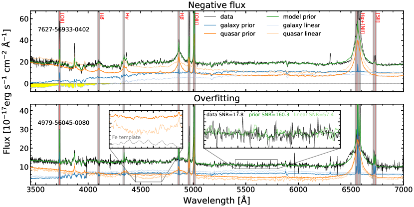
Figure 1: Two examples show typical problems (negative flux and overfitting) in the linear decomposition method. The first example highlights the negative flux of the host galaxy model (yellow regions) in linear decomposition. The second example shows the unrealistic twist and overfitting problem, indicated in insets. Both issues are addressed with our new method; see §2.1 for details. The original spectra are depicted with black lines, while regions with strong emission lines, shaded in gray, are masked during fitting. Our fitted models for the galaxy and quasar are represented in dark blue and orange lines, respectively, with the combined model displayed in green. For comparison, the results from linear decomposition are shown in light blue and orange. Spectral names (plate, MJD, fiber), line names, SNR are listed.

The PCA, also known as the Karhumen-Loève transformation, is a mathematical method usually used for dimensionality reduction, transforming high-dimensional data into a lower-dimensional space. The fundamental concept is to find a lower-dimensional set of orthogonal eigenvectors where the projection of the original data can preserve most of its characteristics. In spectral analysis, each spectrum can be thought of as a vector in a multidimensional hyperspace, with each wavelength pixel representing one axis, $\hat{\lambda}_{j}$. Then the $i$th spectrum can be expressed as $\mathbf{f}_{i}=\sum_{j}{f_{ij}\hat{\lambda}_{j}}$, where $f_{ij}$ is the spectral flux at $\hat{\lambda}_{j}$. Similarly, we can define a set of rotated base vectors, $\mathbf{e}_{k}=\sum_{j}e_{jk}\hat{\lambda}_{j}$, where $k$ is the index of the base vector. Thus, the original spectra can also be expressed as $\mathbf{f}_{i}=\sum_{k}{f^{\prime}_{ik}}\mathbf{e}_{k}$, where $f^{\prime}_{ik}=\sum_{j}{f_{ij}e_{jk}}$. Given a sample of spectra, the PCA aims to identify a set of base vectors that maximize the variance of the projections of the original data onto these vectors in a sequential manner: the first base vector captures the highest variance, denoted by $\sigma^{2}_{f^{\prime}_{i1}}$, followed by the second base vector, which accounts for the next highest variance, and so forth. We call this set of basis vectors as the eigenspectra. Since the eigenspectra are usually built based on populations with similar characteristics, ideally, the first few eigenspectra would account for nearly all information (variance) (Vanden Berk et al., 2006).

In astronomy, the PCA technique is extensively used for spectral classification and dimensionality reduction (e.g., Connolly et al., 1995; Ronen et al., 1999; McGurk et al., 2010; Pâris et al., 2011; Ma et al., 2019). Yip et al. (2004a, b) and Li et al. (2005) have demonstrated that, for galaxies, the first five eigen spectra can account for over 98% of the variance, while for quasars, the first ten eigenspectra can explain more than 90% of the variance. If AGN spectra are simple combinations of emissions from quasars and galaxies, integrating the PCA spectra of both allows us to effectively separate two components from the composite spectra (Vanden Berk et al., 2006; Shen et al., 2008). Thus, the method of decomposing using a linear combination of PCA spectra has been widely adopted in various studies due to its computational efficiency and stability (e.g., Shen et al., 2015; Sun & Shen, 2015; Rakshit et al., 2020).

However, when these methods are applied to a large quasar sample with relatively low spectral SNR of $\sim$ 5, typical of current spectroscopic surveys, the failure rate of such decompositions increases significantly (Rakshit et al., 2020). Moreover, even for high SNR spectra, there remains a substantial failure rate. We emphasize that these failures stem not only from extremely low host galaxy fractions, but also from significant contributions of model degeneracies and overfitting.

Fig. 1 exhibits two typical examples of the unreliable decomposition results using 10 quasar eigenspectra and 5 galaxy eigenspectra. Negative model is the most common problem that leads to failure in linear decomposition, as shown with at the shorter wavelength range in the upper panel (also see Fig. 3). Even for some cases where the decomposed models are entirely positive, they might still be physically unreal solution, e.g., absorption features erroneously appearing in regions typically characterized by emission lines. These issues are often caused by competition between two sets of PCA templates. If one set overestimates the flux, the other must compensate by turning negative to offset the excess and align closely with the total data flux.

In the second example, we clearly see a depressed feature in the linearly decomposed quasar model at around 4600 Å (also see the inset), where the original data are smooth and flat. Normally, this region is dominated by a series of broadened Fe ii emission lines, and thus, a flat or convex continuum would be expected. We suggest that the concave decomposed AGN continuum is anomalous, likely resulting from degeneracies. Furthermore, the linear decomposition method tends to overfit the noise within the spectra. Theoretically, the fitted template should maintain a constant SNR level, independent of the data’s SNR. In the second example the linearly decomposed AGN model (light green line) appears significantly noisier than the prior-informed model (dark green line) around 5600 Å (also see the inset). Given the high SNR of the PCA templates, there are no prominent features in this region, and therefore, the fitted model should exhibit a very smooth appearance. The additional noise in the linearly fitted results stems from overfitting the data noise with high-order PCA templates (see §2.3 for details).

The issues mentioned above are primarily due to the simplistic nature of the decomposition method. A critical problem is that although the PCA spectra within the same set are mutually orthogonal and independent, those from two different sets (i.e., quasar and galaxy template libraries) can exhibit severe degeneracy. Furthermore, in cases of low SNR spectra, high-order PCA templates might be used to fit noise artifacts, resulting in their disproportionate weighting in the fitting process (see §2.2.1). Consequently, originally negligible higher-order eigenspectra might compete for flux with the dominant eigenspectra, leading to a disastrously unrealistic solution.

2.2 Prior-Informed PCA Decomposition

To mitigate issues of degeneracy and overfitting, we assign weights to each PCA eigenspectra during the decomposition. These weights are natural byproducts of the construction of PCA templates. We employ the penalized pixel fitting method (e.g., Merritt, 1997) to incorporate these weights into the fitting procedure. By leveraging this approach, we effectively mitigate the degeneracy between different PCA templates and significantly enhance the overall quality of the decomposition. The success rate of this method reaches approximately 94% for the SDSS DR16Q catalog with $z<0.8$.

2.2.1 Distribution of PCA Eigencoefficients

Following Vanden Berk et al. (2006), we chose the quasar PCA templates built based on the C1 bin in Yip et al. (2004a), which has an absolute $i$-band magnitude of $-26<M_{i}<-24$ and a redshift of $0.08<z<0.53$. The low redshift range was selected to match the general population properties of our target sample. The high luminosity of the PCA templates minimizes the host contamination. However, since these PCA templates were constructed based on the first data release (DR1) of SDSS and include a relatively small number of identified quasars (109 objects), they may not fully represent the broader quasar population. While the current templates are sufficient for proof of concept, developing more comprehensive PCA templates (Bailey, 2012), e.g., $z$ up to 1, in a future study could further improve the feasibility and accuracy of the host decomposition (Brodzeller et al., 2023). The galaxy PCA templates used in this study were created by Yip et al. (2004b) and are based on approximately 170,000 galaxies from SDSS DR1.

Following the procedure described in Yip et al. (2004a, b), we collected the spectra used to construct the PCA templates and then projected the data onto each eigenspectrum to obtain the coefficient,

$$c_{i}=\sum_{k}{f_{k}e_{ik}},$$ (1)

where $f_{k}$ is the spectral flux at wavelength $\lambda_{k}$ and $e_{ik}$ is the $i$th eigenspectra value at wavelength $\lambda_{k}$. We retained only the coefficients associated with the first ten eigenspectra and normalized these coefficients for each spectrum to ensure that the sum of their squares equals 1. These normalized coefficients, known as eigencoefficients or weights, are illustrated in the upper panels of Fig. 2. The distributions of the first five eigencoefficients for both the quasar and galaxy samples are presented.

For galaxy and quasar spectra, the first eigenspectrum accounts for over 90% of the total weight, while the second eigenspectrum takes about half of the remaining weight, on average. Assuming that the AGN spectra comprise two independent components (quasar$+$galaxy), we would expect that the normalized eigencoefficients for each component derived from the decomposition process should generally follow the distributions observed in pure quasar and galaxy populations respectively. However, in practice, the linear decomposition method does not guarantee these expected distributions.

In the lower panels of Fig. 2, we apply linear decomposition to quasars from the SDSS DR16Q catalog and present the distribution of the eigencoefficients as color-filled histograms. For comparison, we also display the posterior distribution obtained through our prior-informed method as step histograms, alongside the prior distribution shown in gray histograms. The scatter in the coefficient distribution derived from the linear method is significantly larger than expected, suggesting that this method has overestimated the weights of high-order PCA templates in a substantial portion of the sample. Consequently, we propose using the parameter distribution from the building sample as a prior to constrain the fitting. As illustrated in the figure, our prior-informed method effectively reduces the scatter and confines the parameter distribution within a reasonable range.

In the linear decomposition method, we notice a greater deviation in the parameters for galaxy PCA templates compared to those for quasar PCA templates. This disparity arises because the quasar component typically dominates the total flux, resulting in more stable fitting outcomes. Conversely, the galaxy component is relatively weaker and more sensitive to noise, resulting in more serious fitting degeneracy.

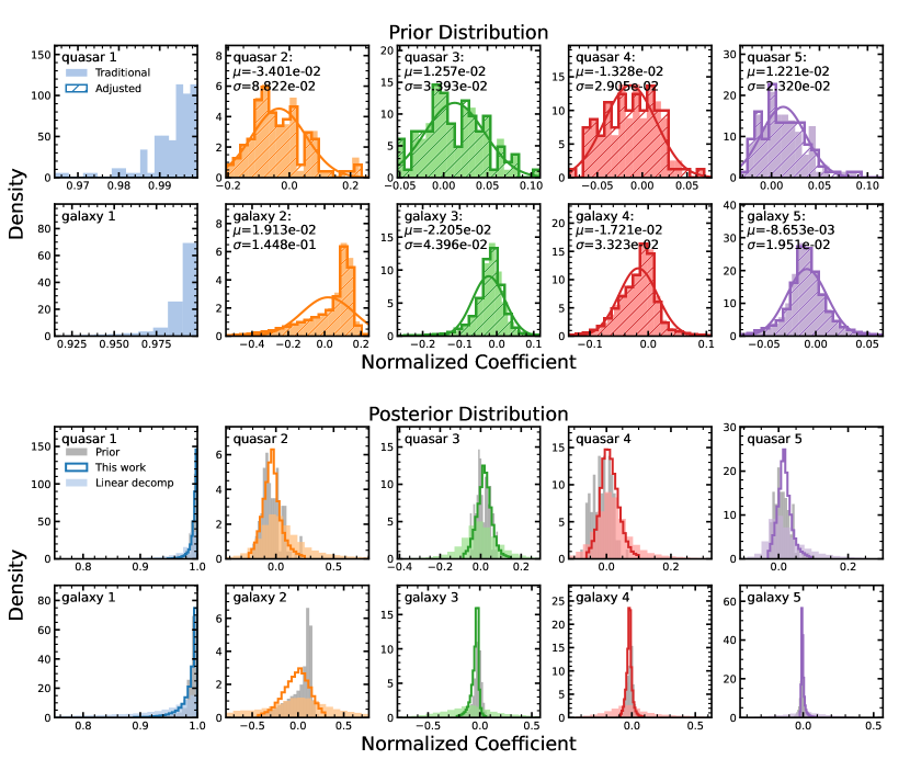
Figure 2: The prior and posterior distributions of the eigencoefficients. The upper panels show the distributions of normalized eigencoefficients for the first five quasar and galaxy PCA templates. The filled (traditional) and dashed (adjusted) histogram represent the distribution of coefficient normalized with different methods (See §2.2.2). Our adjusted method can faithfully recover the traditional distribution and enhance the optimization efficiency. We use one Gaussian to model the adjusted distribution, and the fitted parameters are listed in the upper left. The lower panels show the posterior distributions of eigencoeffcients from prior-informed and the distributions from linear decomposition based on SDSS DR16 quasars. Prior distributions are plotted for comparison. The prior-informed method significantly reduced the fitting degeneracy and the scatter of the eigencoeffcients distribution.

2.2.2 Penalized Pixel Fitting

The fundamental reason for the mismatch between the linear PCA decomposed distributions and the prior distribution stems not only from the degeneracy among PCA templates but also from the overfitting of noise. To resolve this issue, it is crucial to impose self-adaptable constraints on the fitted PCA eigencoefficients, which can change the strength of the constraints according to the spectral SNR. The maximum penalized likelihood formalism used in pPXF provides a solution to this requirement (Merritt, 1997; Cappellari & Emsellem, 2004; Cappellari, 2016, 2023). The basic idea is to incorporate an adjustable penalty term to the $\chi^{2}$ to move the solution towards the prior. The penalty term is only related to the weights of each fitting parameter. The greater the deviation of the weights from the prior, the larger the penalty term becomes. Since the $\chi^{2}$ term is also affected by the spectral SNR, the penalty term would be more dominant in lower SNR cases. By combining these two terms within a balance factor, the program can automatically make a compromise between a lower $\chi^{2}$ and a more prior-like solution.

To construct a uniform penalty term that incorporates both the galaxy and quasar PCA sets, it is necessary to normalize each set of coefficients. Traditionally, this normalization involves:

$$q\prime_{i}=\frac{q_{i}}{\sqrt{\sum_{i=1}^{m}{q_{i}^{2}}}},$$ (2)

where $q_{i}$ and $q\prime_{i}$ represent the eigencoefficients before and after normalization, respectively, and $m$ denotes the total number of templates used. This normalization method is equivalent to setting an implicit constraint to all coefficients, i.e. the sum of the squares of all coefficients equals 1, which would hinder the optimization. Considering the computational costs and convergence efficiency, we use the coefficient of the first eigenspectra as the normalization factor and only use priors to constrain the rest of the coefficients. The normalization formula is then simplified to:

$$q\prime_{i}=\frac{q_{i}}{q_{1}},i\neq 1.$$ (3)

The new distributions of the rest of the coefficients are shown as hatched histograms in Fig. 2. Since the first eigencoefficients in both sets consistently approximate 0.95 with little variation, re-normalizing the subsequent coefficients does not substantially alter the prior distribution.

Given normalized eigencoefficients, we can then parameterize the prior distribution. Except for the first-order eigencoefficients, the rest generally distribute around 0 with a small standard deviation. We thus simply use a normal distribution to represent each prior distribution. The parameter used in this work is listed in Table 1. Apparently, the distributions of the second-order galaxy eigencoefficients are asymmetrical and have a longer tail than the normal distribution. However, the approximation using a normal distribution is sufficiently effective for improving decomposition fitting. Given that the penalty term must be calculated in every iteration of the optimization, employing a complex distribution would substantially increase the computational cost with negligible gain. Additionally, the data size available for quasar PCA templates is not large enough to support a more intricate model. Constructing quasar PCA templates with a data volume comparable to that of galaxy PCA templates, and modeling the distribution using GAMLSS (Generalized Additive Models for Location, Scale, and Shape, Rigby & Stasinopoulos, 2005) or a non-parametric model, would be a promising future work.

With the above preparations in place, we design the penalized $\chi_{p}^{2}$ as

$$\chi_{p}^{2}=\chi^{2}(1+\alpha\mathcal{P}),$$ (4)

where $\alpha$ is the adjustable factor and $\mathcal{P}$ is the penalty function, respectively. Assuming every normalized coefficient $q\prime_{i}=q_{i}/q_{1}~{}(i\neq 1)$ follows a normal distribution, we can fit a mean value $\mu_{\rm q\prime_{i}}$ and a standard deviation $\sigma_{\rm q\prime_{i}}$ from the prior sample. Then, the penalty function can be naturally constructed as:

$$\mathcal{P}=\left(\sum_{i=2}^{m}{\left(\frac{q\prime_{i}-\mu_{q\prime_{i}}}{\sigma_{q\prime_{i}}}\right)^{2}}+\sum_{i=2}^{n}{\left(\frac{g\prime_{i}-\mu_{g\prime_{i}}}{\sigma_{g\prime_{i}}}\right)^{2}}\right)/(m+n-2).$$ (5)

Here, we use $q_{i}$ ($g_{i}$) to represent the $i$th coefficient of quasar (galaxy) PCA template and $m$ ($n$) to represent the total number of used template.

During our fitting, we adopted the penalty factor $\alpha=0.01$, which has the most prior-like posterior distribution. With a larger penalty factor, the fitting procedure would have stronger constraints and resulted in a narrower posterior distribution of the fitted eigencoefficients and vice versa. Nevertheless, the success rate of decomposition and the host fraction would not be significantly affected by changing $\alpha$ from 0.001 to 0.1.

Throughout this work, we use the first 5 PCA components for galaxies and the first 10 PCA components for quasars to perform the decomposition, i.e., $m=10$ and $n=5$, following previous studies (e.g., Vanden Berk et al., 2006; Shen et al., 2008, 2015; Rakshit et al., 2020). As all PCA eigencoefficients are constrained by the prior distributions, incorporating additional higher-order PCA components, which contribute minimally to the overall weight, would not substantially alter our results. Major emission lines are masked during the fitting process to mitigate the model competition effect (gray windows in Fig. 1). We eventually reconstructed the quasar and galaxy eigenspectra, utilizing LMfit (Newville et al., 2014) for minimization, and measured the host galaxy fraction at 5100 Å ($f_{\rm h,5100}$) and 4200 Å ($f_{\rm h,4200}$).

Table 1: Best-fit parameters of the normal distribution for the first 10 normalized PCA eigencoefficients of quasar and galaxy sets.

Order	$\mu_{\rm gal}$	$\sigma_{\rm gal}$	$\mu_{\rm qso}$	$\sigma_{\rm qso}$
1	/	/	/	/
2	$~{}~{}1.91\times 10^{-2}$	$1.45\times 10^{-1}$	$-3.40\times 10^{-2}$	$8.82\times 10^{-2}$
3	$-2.20\times 10^{-2}$	$4.40\times 10^{-2}$	$~{}~{}1.26\times 10^{-2}$	$3.39\times 10^{-2}$
4	$-1.72\times 10^{-2}$	$3.32\times 10^{-2}$	$-1.33\times 10^{-2}$	$2.90\times 10^{-2}$
5	$-8.65\times 10^{-3}$	$1.95\times 10^{-2}$	$~{}~{}1.22\times 10^{-2}$	$2.32\times 10^{-2}$
6	$-1.20\times 10^{-2}$	$2.12\times 10^{-2}$	$~{}~{}4.47\times 10^{-3}$	$1.74\times 10^{-2}$
7	$~{}~{}5.63\times 10^{-3}$	$1.67\times 10^{-2}$	$-1.36\times 10^{-3}$	$2.03\times 10^{-2}$
8	$-4.41\times 10^{-3}$	$1.26\times 10^{-2}$	$-1.36\times 10^{-3}$	$1.16\times 10^{-2}$
9	$-3.45\times 10^{-3}$	$9.84\times 10^{-3}$	$-5.25\times 10^{-3}$	$6.17\times 10^{-3}$
10	$~{}~{}4.85\times 10^{-3}$	$7.82\times 10^{-3}$	$~{}~{}4.21\times 10^{-3}$	$9.57\times 10^{-3}$

2.3 Benchmark Tests

2.3.1 Efficiency

Utilizing a comprehensive stellar library as the host template for performing host spectral decomposition is a relatively robust approach. This method fits all components simultaneously and employs an MCMC technique to ascertain the global optimum (e.g., Sexton et al., 2021). However, the extensive computational demands of the MCMC method, which typically require several hours per spectrum, making it impractical for large-scale studies that involve tens of thousands of quasar spectra.

The prior-informed decomposition proposed by this paper is more economical. The entire fitting procedure, combining the decomposition process, host galaxy fitting with pPXF, and quasar spectra fitting with PyQSOFit, only requires a few minutes for a single computational core to execute 100 Monte Carlo simulations to assess statistical uncertainties. To avoid convergence at a local minimum, we run decomposition with initial host fractions from 0.1 to 0.9 in increments of 0.1 for each spectrum and adopt the result with the lowest $\chi^{2}$. The overall resource consumption of our pipeline approximately triples that of the original PyQSOFit, which adopts the linear combination decomposition method.

2.3.2 Efficacy

Figure 3: Upper panel: The number density distribution of original sample used in decomposition. Middle panel: The success rate of different decomposition methods as a function of spectral SNR. Blue circles represent our prior-informed method; orange triangles stand for the linear decomposition method using quasar PCA templates based on the C1 sample (a low redshift and high luminosity quasar sample) in Yip et al. (2004a); green squares denote the linear decomposition method using global quasar PCA templates. Lower panel: the mean SNR of reconstructed model of all successfully decomposed spectra as a function of spectral SNR. If the model is not overfitting to spectral noise, a uniformly high spectral SNR of the model is expected.

The decomposition success rate and the ability to avoid overfitting noise are two key evaluation metrics for our method. To assess the efficacy of our approach, we applied our decomposition process to the low-redshift subset of SDSS DR16 quasars, which comprise a total of 76,565 quasars with $z<0.8$ (see §3.1 for details).

Given the definition of failed host decomposition, where the fitted galaxy or quasar templates exhibit more than 10% negative pixels, we assessed the efficacy of our prior-informed method across different spectral SNRs, compared with that of linear decomposition methods, as shown in Fig. 3. Two different templates are used in the linear decomposition method: the C1 bin and global quasar PCA templates. As previously mentioned, the former is built from a low-redshift, high-luminosity subsample, adopted in our developed decomposition method. The latter is the default template used in previous versions of PyQSOFit, and was constructed from all quasar spectra in SDSS DR1, covering a redshift range up to $\sim$ 5 and a wavelength span from 900 to 8000 Å. The spectral SNRs are calculated using a data-based algorithm, DER_SNR (Stoehr et al., 2008), which provides a simple and robust estimation for spectra with varying wavelength coverage, without relying on pixel errors.

The middle panel of Figure 3 illustrates two significant improvements achieved through our prior-informed decomposition approach: Firstly, the success rate of our method has significantly improved across all spectral SNR regimes, outperforming the linear decomposition. Secondly, by incorporating a penalty function and C1 quasar PCA templates, we effectively mitigate the degeneracy issue in most SDSS quasars, particularly at the low SNR end (less than 5). This has elevated the success rate from $<$ 60% to $>$ 90%.

The difference of using different PCA templates is clearly demonstrated in two distinct linear decompositions (C1 and global). Although global quasar PCA templates are generally considered more representative of typical quasars, the inclusion of low-luminosity quasars in their constructed sample introduces potential host features. These features compete with the galaxy PCA template, leading to failed decompositions. Additionally, during the decomposition process, a significant portion of the global PCA template must be truncated, further exacerbating the degeneracy issue. Consequently, it is not surprising that the success rate of the global PCA templates is lower than that of the C1 bin templates.

For the prior-based results, the success rate decreases with increasing spectral SNR. This occurs because high-SNR spectra retain finer structures, necessitating either a greater number of templates or a more intricate model for accurate fitting. While increasing the number of PCA templates used in decomposition can improve the success rate for high-SNR spectra, it also decreases the success rate for low-SNR spectra. Moreover, the limited representativeness of the C1 bin quasar PCA templates, based on only 109 quasars, could be a significant factor contributing to the lower success rate.

The lower panel of Fig. 3 displays the spectral SNR of reconstructed model for all successfully decomposed objects as a function of the SNR of its spectral data. Ideally, if the model is not overfitted to spectral noise, we would expect a uniform template SNR in the reconstructed model, regardless of the observed spectral SNR. The figure clearly shows that the template SNR from all three methods remains stable around 160 at the high SNR end, indicating that the PCA templates used in this work are effective in recovering spectra with SNRs greater than 10. At the low SNR end, the template SNR from linear decomposition methods decreases sharply, confirming the overfitting issue previously discussed in §2.1. In contrast, the template SNR based on the prior-informed method remains stable at a high level, indicating that the overfitting issue is significantly reduced.

2.3.3 Host Fraction Accuracy

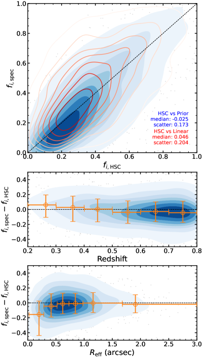
Figure 4: The comparison of $i$-band host fractions between the Hyper Suprime-Cam Subaru Strategic Program (HSC-SSP) image decomposition (Li et al., 2021a) and this study in the observed frame. In the upper panel, we directly compare the results of 2651 quasars in our sample having HSC images. As a comparison, linear decomposition method is also plotted as red contours. The host fraction difference dependence on redshift and effective radius of host galaxy are shown in the middle and lower panels. We show the binned median with orange circles. Their x-axis error indicate the bin size and their y-axis error indicate the 16% to 84% range.

To verify the precision of our host decomposition, we compare our results with those from high-quality image decomposition. Li et al. (2021a) have compiled an AGN-host decomposition catalog from the Hyper Suprime-Cam Subaru Strategic Program (HSC-SSP). This catalog is a subsample of the SDSS DR14Q catalog (Pâris et al., 2018). For comparison, we applied the HSC $i$-band filter transmission function to our decomposed host galaxy template and the original spectra to determine the spectral host fraction in the HSC $i$-band, $f_{i}$. For the HSC images, we convolved the HSC decomposition model with a 2-D Gaussian with an FWHM equal to the median plate seeing and then applied a circular aperture (2″ diameter for BOSS spectra and 3″ diameter for SDSS spectra) to each model to derive a fiber-corrected host fraction. This process yielded 2651 quasars with valid host fraction measurements in both catalogs, whereas only 1560 of them can be decomposed using the linear decomposition method due to its relatively low success rate.

The upper panel of Fig. 4 illustrates the comparison between the host decomposition results using the prior-informed method (blue contours) and the linear decomposition method (red contours). Employing the image decomposition results as a benchmark, the prior-informed method achieves a median offset of $-0.025$ and a scatter of 0.173, while the linear method records a median offset of 0.046 and a scatter of 0.204. This suggests that the prior-informed method has significantly improved the success rate of decomposition and reduced the scatter in host fraction measurements, albeit with a slightly median offset, which should originate from intrinsic uncertainties in different methods and datasets.

The two lower panels of Fig. 4 demonstrate that the differences between spectroscopic and image decompositions generally show no dependence on the redshift and effective radius of the host galaxy. The drop-off in differences for host galaxies with an effective radius less than $0.5\arcsec$ suggests that image decomposition may compete with the AGN model in compact galaxies, leading to an overestimation of the host fraction. Such a discrepancy could be reason for the weak decreasing trend in these differences relative to redshift, which the galaxy size would be smaller at higher redshifts.

2.3.4 Stellar Velocity Dispersion Accuracy

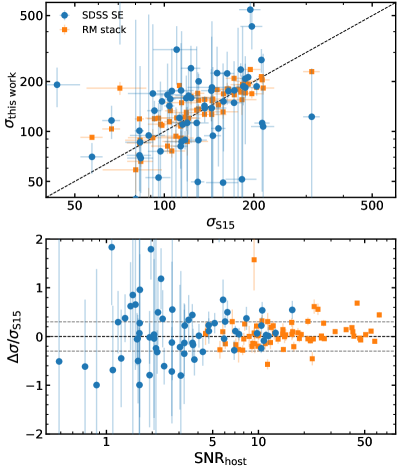
Figure 5: The comparison of stellar velocity measurements given by Shen et al. (2015) and by this work. We apply our fitting routine to the best single-epoch spectra (SDSS SE) and the stacked high SNR spectra (RM stack) of these reverberation-mapping targets and give two sets of stellar velocity measurements. We present the direct comparison in the upper panel and the dependence of differences on the host galaxy spectra SNR in the lower panel. The gray dashed horizontal lines in the lower panel indicate the $\pm$ 30% difference limits.

The stellar velocity dispersion $\sigma_{\star}$ is crucial for studying host galaxy properties. We evaluate the accuracy of our method in $\sigma_{\star}$ measurements by fitting the host component using the stellar kinematics fitting code pPXF (see §3.2 for details).

To assess the accuracy of our $\sigma_{\star}$ measurements, we compare our results with those of 66 high-quality RM stacked quasar hosts cross-matched from Shen et al. (2015). To evaluate the performance of our method across both low and high spectral SNRs, we apply our routine to both the stacked RM spectra and the corresponding best SE spectra (labeled as Science Primary in SDSS archives) for each object. Fig. 5 presents our measured velocity dispersions, which are generally consistent with the stacked spectra (mostly within 30%). However, the measurement is very sensitive to the spectral SNR. When switching to SE spectra with relatively lower SNRs, the inconsistency increases significantly, especially when spectral $\rm SNR_{host}<4$. Therefore, we suggest that a minimum criterion of ${\rm SNR_{host}}>4$ is required when using the $\sigma_{\star}$ measurements in our catalog.

3 Application

The benchmark tests have demonstrated that our algorithm not only achieves a high success rate but also effectively mitigates overfitting issues. We thus applied our method to the entire low-redshift SDSS DR16 quasars. This section briefly outlines the data and spectral analysis methods employed. Subsequent discussions present the results of our measurements and explore the impact of host galaxy emission on existing AGN studies.

3.1 Data and Sample Selection

The SDSS DR16Q catalog, compiled by Lyke et al. (2020), represents the final quasar sample from SDSS IVand includes 750,414 quasars. The majority of the spectra were observed by BOSS spectrographs (Smee et al., 2013), which cover a wavelength range from 3600 to 10,400 Å at a spectral resolution $R\sim$ 2000. The remaining spectra ($<$10%) were obtained using SDSS I/II spectrographs with a shorter wavelength coverage of 3800 to 9200 Å. Given that the host galaxy’s contribution is relatively low in distant, bright quasars, we limited our sample to a redshift of $z<0.8$. This threshold ensures the inclusion of the H$\beta$ emission line region and the 5100 Å luminosity, which are critical for estimating $M_{\rm BH}$. This criterion yields 76,565 quasars for further study.

3.2 Spectral Analysis

Our fitting procedure is based on the open-source spectral fitting code PyQSOFit (Guo et al., 2018). The prior-informed decomposition method has already been merged into the GitHub repository. In the pipeline, the spectra are first corrected for Galactic extinction using a dust map by Schlegel et al. (1998) and a Milky Way extinction curve from Fitzpatrick & Massa (1990), and then transformed to the rest frame based on the redshift identified in DR16Q (Lyke et al., 2020). Next, we utilize both the galaxy and quasar PCA spectra (Yip et al., 2004a, b) to perform the prior-informed decomposition, separating the host galaxy and quasar components. For more details, also see Shen et al. (2011, 2019).

3.2.1 Measurements of the Host Galaxy properties

The host galaxy spectra are derived by subtracting the reconstructed quasar eigenspectra from the original spectra (galaxy = data $-$ quasar templates). Due to the complexity of the broad component of the quasar spectra, the quasar PCA templates may not fully recover the broad line shape. To minimize the impact of residual broad H$\alpha$ and H$\beta$ emission lines, we mask out the regions from 6400$\sim$6765 Å and 4760$\sim$5035 Å in the host galaxy spectra. For a conservative result, the pixel error from the original spectra is directly adopted as that of the host galaxy spectra in our subsequent measurement error estimations, which is apparently overestimated.

We then employ the stellar kinematics fitting code pPXF to measure the stellar velocity dispersion ($\sigma_{\star}$) of the host galaxy. The Indo-U.S. Library of Coudé Feed Stellar Spectra (Valdes et al., 2004) was adopted as the stellar library, which covers the wavelength of 3460$\sim$9460 Å at a spectral resolution of 1.35 Å. We broaden the templates to the SDSS spectral resolution (2.76 Å) before fitting. Only the first two moments (radial velocity and velocity dispersion) are fitted. Uncertainties are derived from the standard deviation of 100 mock spectra generated by adding Gaussian noise realization to the host galaxy spectra.

Since our sample spans a large redshift range, to guarantee the consistency of our measurements, we restrict the fitting range to 4000 $-$ 5350 Å, the same as used in Shen et al. (2015). A few significant stellar absorption features are within this range, including the G band (4304 Å), the Mg i b $\lambda\lambda$5167, 5173, 5184 triplet, and Fe I blends (5270 Å). The preferred infrared Ca ii $\lambda\lambda$8498, 8542, 8662 triplet around 8500 Å falls outside the PCA templates used in this work. Additionally, the unreliable Ca H+K $\lambda\lambda$3969, 3934 line is excluded due to its strong dependence on spectral type, its location in a region with a steep local continuum, and significant intrinsic broadening, as noted in Greene & Ho (2006).

We also measure the ${\rm D_{n}}4000$ index, defined as the flux ratio of two adjacent windows: 3850$\sim$3950 Å and 4000$\sim$4100 Å (Balogh et al., 1999). Its value increases as a function of stellar population age (e.g. Kauffmann et al., 2003b; Zahid et al., 2015; Zahid & Geller, 2017), thus serving as an age indicator of the host galaxy.

3.2.2 Measurements of the Quasar Properties

The quasar spectra are also derived by using the original spectra and subtracting the reconstructed galaxy eigenspectra (quasar = data $-$ galaxy templates). To avoid the blending of emission and absorption lines from hosts, we simply assume that the total emission line flux, e.g., H$\beta$ and [O iii], is from quasars, ignoring the negligible contributions from the hosts.

The quasar spectral fitting procedure is similar to previous works (Shen et al., 2019; Guo et al., 2019; Ren et al., 2022; Wu & Shen, 2022). Here, we describe the general workflows and fitting setups. First, we fit the dereddened, deredshifted quasar spectra in several line-free regions using a power-law model along with a broadened empirical optical Fe ii emission line template (Boroson & Green, 1992). After subtracting the continuum models, we fit the emission lines using Gaussian profiles on the emission-line-only spectrum. For the H$\alpha$ complex, we employ 3 Gaussian models to fit the broad components and 1 Gaussian for each narrow line including H$\alpha$, the [N ii] doublet, and the [S ii] doublet. Similarly, for the H$\beta$ complex, we use 3 Gaussian models for the broad H$\beta$ component and 1 for narrow H$\beta$. A core component and a wind component are considered for each [O iii] doublet. The relative line centers and line widths are fixed during the fitting for narrow lines and the wing components, respectively.

3.3 Results

We compiled our spectral measurements in Table 2. Out of 76,565 low-redshift quasars, we successfully performed host decomposition for 71,760 quasars (93.7%). In the following sections, we use the host fraction at 5100 Å to represent the host contribution, unless specified otherwise. As a comparison, the decomposition success rate in Rakshit et al. (2020), which uses the linear decomposition method, is only 23% (12,807 out of 55,703). Next, we compare our refined measurements of AGN to those that do not properly separate the host-AGN components.

3.3.1 Host Galaxy Fraction $f_{h}$

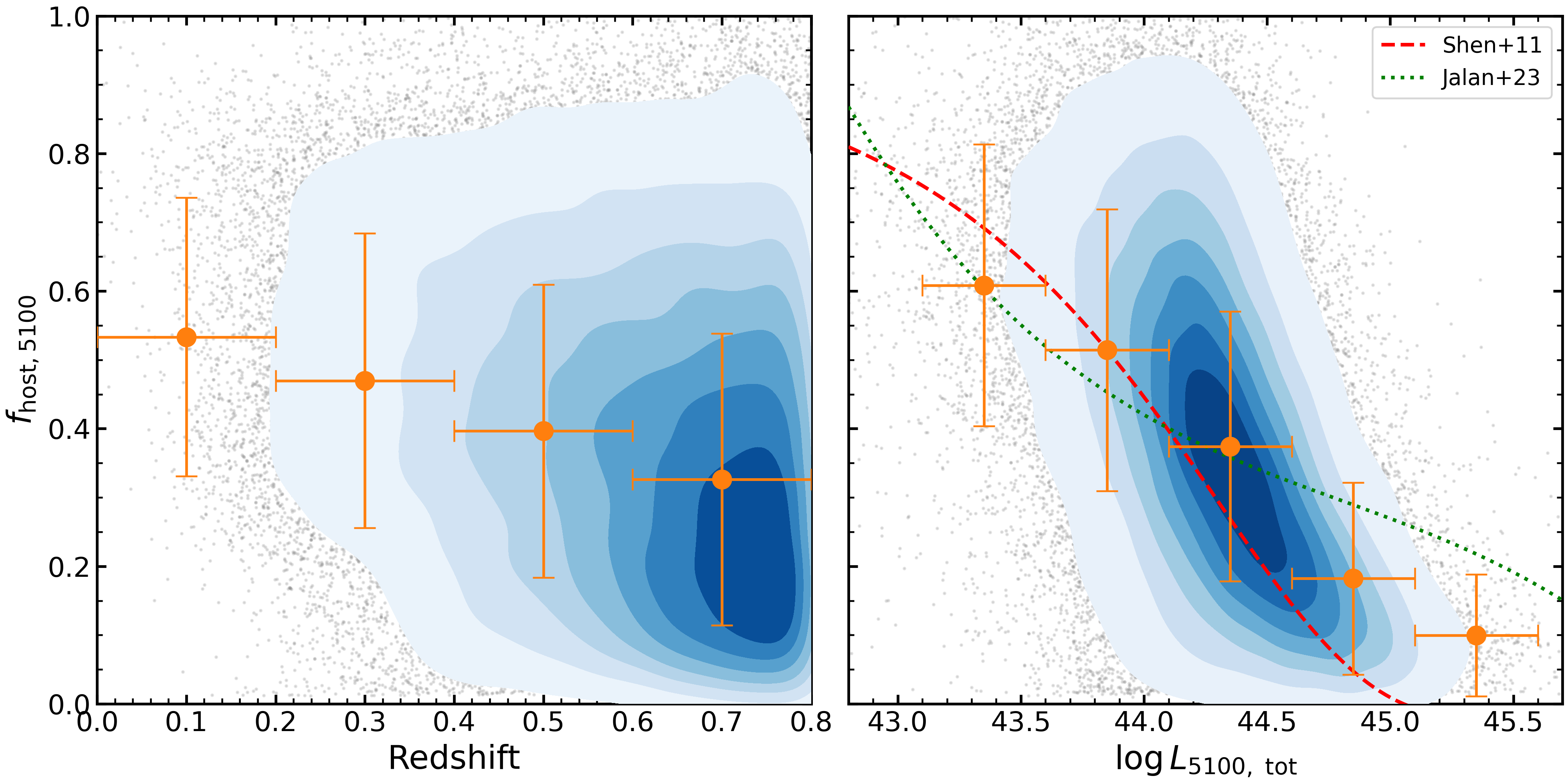
Figure 6: 2D distributions (blue contours) of host fraction at 5100 Å as a function of the redshift and total 5100 Å luminosity. The orange dots show the $f_{\rm host,5100}$ distribution in different redshift and luminosity bins. The x-axis error bars indicate the bin range, and the y-axis error bars indicate the standard deviation of each bin. The red dashed and green dotted lines are previous results for comparison.

The host contribution in the continuum can be significant for low-redshift quasars in SDSS (e.g., Jalan et al., 2023). For all SDSS spectra with $z<0.8$, the median host contribution is $f_{h,5100}=35.7\%$, consistent with the results from SDSS-RM data, which report a median fraction of $38.8\%$ for a similar redshift range (Shen et al., 2019).

Fig. 6 displays the distributions of $f_{\rm host,5100}$ against redshift and total luminosity, $L_{\rm 5100,tot}$, along with the median for each x-axis bin. The host fraction gradually decreases from over 50% at $z\sim 0.1$ to approximately 30% at $z\sim 0.8$. This mild decline in host fraction with redshift could be due to a selection effect at higher redshifts, where only luminous quasars can be identified. Nevertheless, there is no effective redshift cut to avoid host contamination at optical wavelength.

The correlation between the host fraction and the total luminosity is more significant, with a decrease trend in median host fraction of $\sim 65\%$ for the lowest luminosity bin ($L_{\rm 5100,tot}<43.6$) to $\sim 10\%$ for the highest luminosity bin ($L_{\rm 5100,tot}>45.1$). This further confirms the selection effect that a less fractional host component decomposed in a more luminous target at a higher redshift. Two empirical relations suggested by Shen et al. (2011) and Jalan et al. (2023) are also plotted for comparison, which show similar trends to our results. The slight discrepancies among these studies are likely due to the using of different samples and decomposition methods. Generally, catalogs for low-redshift SDSS quasars should be used with caution if the host galaxy is not properly subtracted.

3.3.2 Black Hole Masses

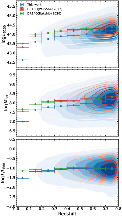
Figure 7: The distributions of measured $L_{5100}$, $M_{\rm BH}$, and Eddington ratio as a function of redshift are depicted for the DR16 quasar catalog (Wu & Shen, 2022), DR14 quasar catalog (Rakshit et al., 2020), and the current study. The filled blue contours represent our results, while the red contours correspond to DR16. Additionally, we bin the sample into intervals of 0.1 in redshift, displaying the corresponding median values for each bin. The difference in $L_{5100}$ comes from the host galaxy subtraction, while the difference in $M_{\rm BH}$ is a combined result of the host galaxy subtraction, the different mass recipe, and the improved FWHM measurements (See §3.3.2).

In this section, we provide the $M_{\rm BH}$ measurement based on our host-subtracted spectra, and quantitatively compare it with previous studies. Furthermore, we will discuss the potential influence of non-host-subtracted measurements on previously obtained results.

The black hole masses $M_{\rm BH}$ are usually calculated based on the 5100 Å continuum luminosity $L_{5100}$ and H$\beta$ broad emission line width ${\rm FWHM_{H\beta}}$, which is the so-called “single-epoch virial BH mass” estimators:

$$\log{\left(\frac{M_{\rm BH}}{M_{\odot}}\right)}=a+b\log{\left(\frac{L_{5100}}{10^{44}~{}\text{erg s${}^{-1}$}}\right)}+c\log{\left(\frac{\rm FWHM_{H\beta}}{\text{km s${}^{-1}$}}\right)},$$ (6)

where coefficients $a$, $b$, and $c$ are determined empirically using the RM AGN sample (e.g., Vestergaard & Peterson, 2006; Feng et al., 2014; Shen et al., 2019), the fiducial mass recipe, commonly used by quasar studies (e.g., Shen et al., 2011; Rakshit et al., 2020; Wu & Shen, 2022), originates from Vestergaard & Peterson (2006) and specifies coefficients $a=0.91$, $b=0.50$, and $c=2.0$. However, it does not correct for host contributions. Therefore, in this work, we adopted the host-corrected recipe derived by Shen et al. (2023, hereafter S23), which modifies $a$ to 0.85 only. The statistical uncertainties of $M_{\rm BH}$ are given by the propagation of uncertainties in $L_{5100}$ and ${\rm FWHM_{H\beta}}$. For individual quasars, an absolute systematic uncertainty of approximately 0.35 dex in SE masses should be considered (Shen et al., 2023). The bolometric luminosity is estimated using $L_{\rm bol}=9.26\times L_{5100}$, where 9.26 is the bolometric correction obtained from Richards et al. (2006). The Eddington ratio $\lambda_{\rm Edd}=L_{\rm bol}/L_{\rm Edd}$, where $L_{\rm Edd}$ is the Eddington luminosity.

We then compare our revised $L_{5100}$ and $M_{\rm BH}$ measurements with those from Wu & Shen (2022), which did not account for host contributions. Fig. 7 displays the distributions of these two samples as a function of redshift, overlapped the median value for each redshift bin. Considering host emissions, our results show a median $L_{5100}$ that is 0.215 dex lower and a median $M_{\rm BH}$ that is 0.219 dex lower compared to the values reported in Wu & Shen (2022). Despite these differences, the Eddington ratios between the two samples remain consistent, likely due to coincidence. Fig. 7 also includes the distribution from the SDSS DR14Q property catalog (Rakshit et al., 2020) for comparison, which adopted the linear decomposition method with global quasar PCA templates. The discrepancies observed may be attributed to differences in the samples and the low success rate of decomposition in DR14Q.

Several factors contribute to the systematically lower $M_{\rm BH}$, measured as 0.219 dex lower in our study. Firstly, the constant $a$ in the S23 recipe is 0.06 dex smaller than that in VP06. Additionally, the subtraction of the host contribution, 38.8% on average (see §3.3.1), accounts for another 0.11 dex decrease in $M_{\rm BH}$. The remaining 0.05 dex discrepancy is likely attributable to degeneracy in the spectral decomposition process in different works.

Accurate determination of $M_{\rm BH}$ is crucial for deepening our understanding of AGN dynamics and their coevolution with the surrounding environment. Given the systematic overestimation of $M_{\rm BH}$ in low-redshift quasars, we suggest that previous studies relying on the absolute value of $M_{\rm BH}$ could be biased. For instance, the ratio of $M_{\rm BH}$ to galaxy stellar mass based on SE spectra without host correction (e.g., Ding et al., 2020; Li et al., 2021b), might be overestimated compared to local results, where $M_{\rm BH}$ is dynamically measured and relatively free from host contamination. A similar issue exists in estimating the black hole mass function (BHMF): Previous studies often set a redshift limit of $z>0.3$ to minimize host contamination on $M_{\rm BH}$ measurements (Shen & Kelly, 2012; Kelly & Shen, 2013), which, according to our results, is not sufficient. Considerable bias in $M_{\rm BH}$ estimation persists even up to $z\sim 0.8$, raising concerns for BHMF studies using SE mass estimations.

3.3.3 $M_{\rm BH}$-$\sigma_{\star}$ Relation

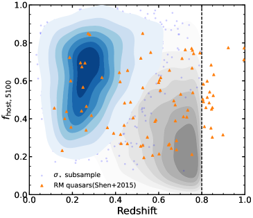
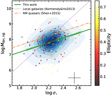
Figure 8: Upper panel: sample distribution in the $f_{\rm host,5100}$-redshift plane. Blue contours and dots represent the quasar subsample that passed the $\sigma_{\star}$ quality cuts. The distribution of our main sample is shown in gray contours with a vertical dashed line indicating the redshift cut at 0.8. The quasars used in Shen et al. (2015) are shown as orange triangles for comparison. Lower panel: the blue contours show the $M_{\rm BH}-\sigma_{\star}$ relation for the $\sigma_{\star}$ quality cut subsample with its average uncertainty at the lower right corner. The green line and the dashed region indicate the best-fit relation and the 95% confidence band derived by linmix. We add the relation derived by Kormendy & Ho (2013); Shen et al. (2015) for reference. We also cross-matched 151 quasars with HSC image in Li et al. (2021b) and color coded with the ellipticity of the host galaxy to illustrate the galaxy inclination effect on $\sigma_{\star}$ measurements.

Given the high success rate of our host decomposition method, we are able to investigate the $M_{\rm BH}$-$\sigma_{\star}$ relation across a larger sample. To ensure the measurement reliability of the stellar velocity dispersion $\sigma_{\star}$, we use the same criteria as Shen et al. (2015): 1) the host fraction at 4200 Å is required to be larger than 0.05; 2) The spectral SNR of host galaxy should be larger than 4; 3) $\sigma_{\star}$ is above $3\sigma$ confidence level (see §2.3.4 for the discussion of the reliability of our $\sigma_{\star}$ measurements).

In total, 4137 quasars passed these quality cuts. The distribution of this subsample in the $f_{\rm host,5100}$-redshift plane is shown in the upper panel of Fig. 8. Different from the main sample, this selection criteria favor quasars with relatively higher host fraction and lower redshift. The median redshift and the median host fraction of this subsample are 0.27 and 63%, respectively. Although we discard most of the high-redshift quasars, this subsample still has a reasonable completeness at low redshift (e.g., 45% for $z<0.3$).

Start from $\sigma_{\star}$ quality cut subsample, we further studied the relation between their $\sigma_{\star}$ and $M_{\rm BH}$ based on broad H$\beta$ line. We use linmix, a Bayesian linear regression code based on the method developed by Kelly (2007), to perform the linear fit:

$$\log{\left(\frac{M_{\rm BH,H\beta}}{M_{\odot}}\right)}=\alpha+\beta\log{\left(\frac{\sigma_{\star}}{200~{}\text{km s${}^{-1}$}}\right)}.$$ (7)

To account for the scatter due to the systematic errors in SE mass estimates, we additionally add 0.35 dex to the measured statistical errors (Shen et al., 2023) during the fitting. The lower panel of Fig. 8 presents the best-fit linear relation, with an intercept of $\alpha=7.940\pm 0.010$ and a slope of $\beta=1.231\pm 0.069$ (green line). The intrinsic scatter of $\log{M_{\rm BH}}$ around the best-fit model is 0.129.

Our result holds a similar slope to that from stacked RM quasar sample (orange dash-dotted line, Shen et al., 2015), yet with $\sim 0.5$ dex lower in $M_{\rm BH}$. The difference in intercept is primarily due to the sample differences in redshift and host fraction, shown in the upper panel of Fig. 8. Since the quasars spectra in Shen et al. (2015) are stacked from about 38 epochs with the accumulated exposure time tens of times higher than that of our SE spectra, their high SNR allows a higher completeness at higher redshift and lower host fraction under the same selection criteria. On the contrary, our sample would favor quasars with relatively lower AGN luminosity and higher galaxy luminosity, leading to a systematic lower-right shift in Fig. 8. Besides, the new recipe for SE $M_{\rm BH}$ estimation and the reduction of host contamination would also contribute to $\sim 0.2$ dex discrepancy, as clarified in §3.3.2.

Our $M_{\rm BH}$-$\sigma_{\star}$ relation is significantly shallower than the local relation for inactive galaxies (purple dotted line, Kormendy & Ho, 2013). The divergence from the local relation is more complex. One frequently cited factor is the luminosity constraints, under which more luminous quasars with brighter broad lines are preferentially identified. Assuming a positive correlation between luminosity and $M_{\rm BH}$, this selection bias leads to a more massive $M_{\rm BH}$-biased sample with respect to $\sigma_{\star}$ (Lauer et al., 2007). In a flux-limited sample, such an offset becomes more pronounced at lower $\sigma_{\star}$ values, resulting in a shallower slope in the $M_{\rm BH}-\sigma_{\star}$ relation (Shen et al., 2015). Note that the redshift of our sample is generally lower than 0.4, so the bias described by Lauer et al. (2007) would be less severe than that in the sample of Shen et al. (2015).

The decomposition procedure would introduce additional uncertainties to the $\sigma_{\star}$ measurements beyond the statistical error. Passing underestimated error could lead to a shallower fitted slope

The accuracy of $\sigma_{\star}$ measurements will also impact the fitted slope. Underestimating the $\sigma_{\star}$ error due to the decomposition procedure, beyond mere statistical errors, and passing this underestimated error to the fitting process could lead to a shallower fitted slope. Besides, the $\sigma_{\star}$ estimation of a subset of our sample could be overestimated, which would extend the true $\sigma_{\star}$ distribution to the right in Fig. 8, and therefore shallow the fitted slope. The measured integrated velocity dispersion from the spectrum is contributed to by both the inner bulge stellar velocity dispersion and the rotational velocity from the outer disk. As will be discussed in §3.3.4 that the AGN hosts tend to be star-forming galaxies, which are likely to be disk dominated. Therefore, the measured dispersion will represent the intrinsic $\sigma_{\star}$ only for face-on galaxies, while being boosted by the rotational velocity for edge-on galaxies, leading to an overestimation of $\sigma_{\star}$ (Bezanson et al., 2015). Fig. 8 highlights 143 quasars with morphology measurements in Li et al. (2021b), color coded by the ellipticity ($\epsilon=1-b/a$) of the host galaxy, which is correlated with the inclination angle. Galaxies with higher ellipticity tend to reside on the right side of the local relation, indicating a possible overestimation of $\sigma_{\star}$.

The potential evolution of the $M_{\rm BH}-\sigma_{\star}$ relation may also play a role in this divergence. Silverman et al. (2022) suggest an intrinsic shallower $M_{\rm BH}-\sigma_{\star}$ slope at higher redshift based on the SDSS quasar at $0.2<z<0.8$, with selection bias corrected. Since the quasars in our sample have a median $z\sim 0.3$, the change of intrinsic relation can be a possible reason.

3.3.4 Stellar Age of Quasar Hosts

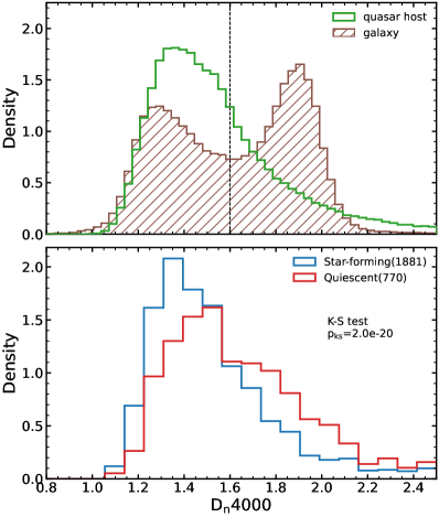
Figure 9: The upper panel shows the distribution of ${\rm D_{n}}$4000 index for our decomposed quasar hosts. The distribution of the ${\rm D_{n}}4000$ index for the galaxy sample used to build the galaxy PCA template is also plotted (hatched histogram) for comparison. Quasar hosts generally reside on the left side of the distribution, consistent with the younger age of the star-forming galaxy population. Quasar hosts with HSC-based $\rm{UVM_{\star}}$ diagram classification (Li et al., 2021b) are displayed in the lower panel, separated by image-based galaxy type. The number of quasars in each bin is listed in the legend.

Previous studies have demonstrated that quasars are predominantly hosted by young galaxies, indicating that the BH accretion rate tracks the star formation rate over cosmic history (e.g., Kormendy & Ho, 2013; Matsuoka et al., 2013; Trump et al., 2013; Xie et al., 2021). The ${\rm D_{n}}$4000 index, a commonly used age indicator, measures the break strength at 4000 Å and reflects the age of host galaxies. This index is typically smaller than 1.6 for young stellar populations and higher than 1.6 for older ones (Kauffmann et al., 2003b). The upper panel of Fig. 9 clearly illustrates a young distribution among our quasar hosts (green histogram), generally consistent with the host ages of X-ray selected Type 2 AGNs that has little contamination from AGN continuum (Silverman et al., 2009; Ni et al., 2023). Our results not only confirm the existing findings that cold gas serves as a common fuel for the SMBH in quasars, but also validate our host decomposition method as reliable for obtaining host properties.

We further checked our measured ${\rm D_{n}}$4000 index of star-forming and quiescent galaxies, identified by HSC image-based $\rm{UVM_{\star}}$ diagram (Li et al., 2021b), in our sample. The lower panel of Fig. 9 shows a significant difference between two groups, with a K-S test p-value of $2.0\times 10^{-20}$. Despite a considerable overlap, this classification of the star-forming and quiescent galaxy populations can be verified by the ${\rm D_{n}}$4000 index from our method, further demonstrating the credibility of our host galaxy decomposition.

4 Summary

We introduced a prior-informed AGN-host spectra decomposition technique which is now implemented in PyQSOFit, which significantly increased the decomposition success rate and provided accurate AGN-host flux ratios, host-free $L_{\rm bol}$ and $M_{\rm BH}$ estimations and host galaxy properties ($\sigma_{\star}$ and ${\rm D_{n}}$4000). We applied this method to SDSS DR16 quasars containing 76,565 quasars at $z<0.8$, and, for the first time, compiled a survey-level, host-decomposed catalog.

The main novelty of our host decomposition is to use the distribution of the PCA eigencoefficient as prior information to decrease the degeneracy of PCA templates between quasar and galaxy datasets, and efficiently reduced the overfitting issue. Our decomposition success rate on SDSS DR16 quasar catalog reaches 93.7%, substantially higher than previous works (Fig. 3).

We illustrate that the average host galaxy contribution in these low-$z$ quasar spectra is 38.8% at 5100 Å. If the host galaxy is not taken into account, this will result in an overestimation of 0.215 dex in $L_{5100}$ and 0.219 dex in$M_{\rm BH}$ (Fig. 7), which could lead to biased conclusions for previous related works, such as the $M_{\rm BH}-M_{\star}$ relation and black hole mass function.

We suggest that the $\sigma_{\star}$ measurements are reliable with a scatter of 0.15 dex when host spectral SNR are larger than 4 (Fig. 5). The $M_{\rm BH}-\sigma_{\star}$ relation in our sample is significantly shallower than the local relation (Kormendy & Ho, 2013), however, consistent to that from high-redshift quasar sample (Shen et al., 2015). We argue that both sample selection bias and measurement scatter would affect the fitted slope.

We note that, limited by the sample size and the spectral resolution of current PCA templates, our code is not optimized for quasars with intrinsically low luminosity or high spectral resolution. To adapt this method for compatibility with next generation of spectroscopic surveys such as DESI (DESI Collaboration et al., 2016a, b), 4MOST (de Jong et al., 2014), and PFS (Takada et al., 2014), a new set of PCA or independent component analysis (Lu et al., 2006) templates based on a more complete sample with higher spectral resolution is required for future work.

All products from this work, including the catalog, fitted parameters and quality assurance figure can be accessed from https://zenodo.org/doi/10.5281/zenodo.11376764.

Table 2: FITS catalog format

Number	Column Name	Format	Unit	Description
1	SDSS_NAME	string		Unique identifier from the SDSS DR16 quasar catalog
2	RA	float32	deg	Right ascension (J2000)
3	DEC	float32	deg	Declination (J2000)
4	Z	float32		Redshift
5	PLATE	int32		SDSS plate number
6	MJD	int32		MJD when spectrum was observed
7	FIBER	int32		SDSS fiber ID
8	SN_CONTI	float32		Mean signal-to-noise ratio estimated at 5100 $\rm{\AA}$
9	LOGL5100_TOT	float32	erg s-1	Logarithmic total luminosity at rest-frame 5100 $\rm{\AA}$
10	LOGL5100_TOT_ERR	float32	erg s-1	Error in LOGL5100_TOT
11	RCHI2_DECOMP	float32		Reduced chi-square of the PCA decomposition
12	HOST_FR_5100	float32		Fraction of host galaxy at rest-frame 5100 $\rm{\AA}$
13	HOST_FR_4200	float32		Fraction of host galaxy at rest-frame 4200 $\rm{\AA}$
14	HOST_FR_REST_G	float32		Fraction of host galaxy at rest-frame SDSS g-band
15	HOST_FR_REST_R	float32		Fraction of host galaxy at rest-frame SDSS r-band
16	HOST_FR_OBS_G	float32		Fraction of host galaxy at observer-frame SDSS g-band
17	HOST_FR_OBS_R	float32		Fraction of host galaxy at observer-frame SDSS r-band
18	HOST_FR_OBS_I	float32		Fraction of host galaxy at observer-frame SDSS i-band
19	HOST_REST_GMAG	float32	mag	SDSS g-band host galaxy magnitude at rest-frame
20	HOST_REST_RMAG	float32	mag	SDSS r-band host galaxy magnitude at rest-frame
21	HOST_OBS_GMAG	float32	mag	SDSS g-band host galaxy magnitude at observer-frame
22	HOST_OBS_RMAG	float32	mag	SDSS r-band host galaxy magnitude at observer-frame
23	HOST_OBS_IMAG	float32	mag	SDSS i-band host galaxy magnitude at observer-frame
24	SN_HOST	float32		Signal-to-noise ratio of the host galaxy
25	DN4000	float32		${\rm D_{n}}$4000 index of the host galaxy
26	VDISP	float32		Velocity dispersion of the host galaxy measured by pPXF
27	VDISP_ERR	float32		Error in VDISP
28	VOFF	float32		Velocity offset of the host galaxy measured by pPXF
29	VOFF_ERR	float32		Error in VOFF
30	RCHI2_PPXF	float32		Reduced chi-square of the pPXF fitting
31	PL_SLOPE	float32		Slope of AGN power law
32	PL_SLOPE_ERR	float32		Error in PL_SLOPE
33	LOGL5100	float32	erg s-1	AGN continuum luminosity at rest-frame 5100 $\rm{\AA}$
34	LOGL5100_ERR	float32	erg s-1	Error in LOGL5100
35	LOGL4200	float32	erg s-1	AGN continuum luminosity at rest-frame 4200 $\rm{\AA}$
36	LOGL4200_ERR	float32	erg s-1	Error in LOGL4200
37	LOGL3000	float32	erg s-1	AGN continuum luminosity at rest-frame 3000 $\rm{\AA}$
38	LOGL3000_ERR	float32	erg s-1	Error in LOGL3000
39	FE_4435_4685_FLUX	float32	$10^{-17}$ erg s-1 cm-2	Flux of Fe II complex within the 4435-4685 $\rm{\AA}$
40	FE_4435_4685_FLUX_ERR	float32	$10^{-17}$ erg s-1 cm-2	Error in FE_4435_4685_FLUX
41	LOGLBOL	float32	erg s-1	Bolometric luminosity estimated based on LOGL5100
42	LOGLBOL_ERR	float32	erg s-1	Error in LOGLBOL_5100
43	LOGMBH	float32	$M_{\odot}$	Black hole mass estimated based on broad H$\beta$ line
44	LOGMBH_ERR	float32	$M_{\odot}$	Error in LOGMBH_HB
45	LOGLEDD_RATIO	float32		Logarithmic Eddington ratio
46	HA_BR_SNR	float32		Signal-to-noise ratio of broad H$\alpha$ component
47	HA_BR_PEAK	float32	$\rm{\AA}$	Peak wavelength of broad H$\alpha$ component
48	HA_BR_PEAK_ERR	float32	$\rm{\AA}$	Error in HA_BR_PEAK
49	HA_BR_FLUX	float32	$10^{-17}$ erg s-1 cm-2	Flux of broad H$\alpha$ component
50	HA_BR_FLUX_ERR	float32	$10^{-17}$ erg s-1 cm-2	Error in HA_BR_FLUX
51	HA_BR_EW	float32	$\rm{\AA}$	Rest-frame EW of broad H$\alpha$ component
52	HA_BR_EW_ERR	float32	$\rm{\AA}$	Error in HA_BR_EW
53	HA_BR_SIGMA	float32	km s-1	Line dispersion of broad H$\alpha$ component
54	HA_BR_SIGMA_ERR	float32	km s-1	Error in HA_BR_SIGMA
55	HA_BR_FWHM	float32	km s-1	FWHM of broad H$\alpha$ component
56	HA_BR_FWHM_ERR	float32	km s-1	Error in HA_BR_FWHM
57	HB_BR_SNR	float32		Signal-to-noise ratio of broad H$\beta$ component
58	HB_BR_PEAK	float32	$\rm{\AA}$	Peak wavelength of broad H$\beta$ component
59	HB_BR_PEAK_ERR	float32	$\rm{\AA}$	Error in HB_BR_PEAK
60	HB_BR_FLUX	float32	$10^{-17}$ erg s-1 cm-2	Flux of broad H$\beta$ component
61	HB_BR_FLUX_ERR	float32	$10^{-17}$ erg s-1 cm-2	Error in HB_BR_FLUX
62	HB_BR_EW	float32	$\rm{\AA}$	Rest-frame EW of broad H$\beta$ component
63	HB_BR_EW_ERR	float32	$\rm{\AA}$	Error in HB_BR_EW
64	HB_BR_SIGMA	float32	km s-1	Line dispersion of broad H$\beta$ component
65	HB_BR_SIGMA_ERR	float32	km s-1	Error in HB_BR_SIGMA
66	HB_BR_FWHM	float32	km s-1	FWHM of broad H$\beta$ component
67	HB_BR_FWHM_ERR	float32	km s-1	Error in HB_BR_FWHM

References

- Astropy Collaboration et al. (2022) Astropy Collaboration, Price-Whelan, A. M., Lim, P. L., et al. 2022, ApJ, 935, 167, doi: 10.3847/1538-4357/ac7c74
- Bailey (2012) Bailey, S. 2012, Publications of the Astronomical Society of the Pacific, 124, 1015, doi: 10.1086/668105
- Balogh et al. (1999) Balogh, M. L., Morris, S. L., Yee, H. K. C., Carlberg, R. G., & Ellingson, E. 1999, The Astrophysical Journal, 527, 54, doi: 10.1086/308056
- Bentz & Katz (2015) Bentz, M. C., & Katz, S. 2015, Publications of the Astronomical Society of the Pacific, 127, 67, doi: 10.1086/679601
- Bentz et al. (2009) Bentz, M. C., Walsh, J. L., Barth, A. J., et al. 2009, The Astrophysical Journal, 705, 199, doi: 10.1088/0004-637x/705/1/199
- Bezanson et al. (2015) Bezanson, R., Franx, M., & Dokkum, P. G. v. 2015, The Astrophysical Journal, 799, 148, doi: 10.1088/0004-637X/799/2/148
- Boroson & Green (1992) Boroson, T. A., & Green, R. F. 1992, Astrophys. J. Suppl., 80, 109, doi: 10.1086/191661
- Brodzeller et al. (2023) Brodzeller, A., Dawson, K., Bailey, S., et al. 2023, The Astronomical Journal, 166, 66, doi: 10.3847/1538-3881/ace35d
- Calderone et al. (2017) Calderone, G., Nicastro, L., Ghisellini, G., et al. 2017, Monthly Notices of the Royal Astronomical Society, 472, 4051, doi: 10.1093/mnras/stx2239
- Canalizo et al. (2012) Canalizo, G., Wold, M., Hiner, K. D., et al. 2012, The Astrophysical Journal, 760, 38, doi: 10.1088/0004-637X/760/1/38
- Cappellari (2016) Cappellari, M. 2016, Monthly Notices of the Royal Astronomical Society, 466, 798, doi: 10.1093/mnras/stw3020
- Cappellari (2023) —. 2023, Monthly Notices of the Royal Astronomical Society, 526, 3273, doi: 10.1093/mnras/stad2597
- Cappellari & Emsellem (2004) Cappellari, M., & Emsellem, E. 2004, Publ. Astron. Soc. Pac., 116, 138, doi: 10.1086/381875
- Connolly et al. (1995) Connolly, A. J., Szalay, A. S., Bershady, M. A., Kinney, A. L., & Calzetti, D. 1995, Astron. J., 110, 1071, doi: 10.1086/117587
- de Jong et al. (2014) de Jong, R. S., Barden, S., Bellido-Tirado, O., et al. 2014, in Ground-based and Airborne Instrumentation for Astronomy V, ed. S. K. Ramsay, I. S. McLean, & H. Takami (SPIE), doi: 10.1117/12.2055826
- DESI Collaboration et al. (2016a) DESI Collaboration, Aghamousa, A., Aguilar, J., et al. 2016a, doi: 10.48550/ARXIV.1611.00036
- DESI Collaboration et al. (2016b) —. 2016b, doi: 10.48550/ARXIV.1611.00037
- Ding et al. (2020) Ding, X., Silverman, J., Treu, T., et al. 2020, ApJ, 888, 37, doi: 10.3847/1538-4357/ab5b90
- Feng et al. (2014) Feng, H., Shen, Y., & Li, H. 2014, ApJ, 794, 77, doi: 10.1088/0004-637X/794/1/77
- Fitzpatrick & Massa (1990) Fitzpatrick, E. L., & Massa, D. 1990, ApJS, 72, 163, doi: 10.1086/191413
- Fries et al. (2023) Fries, L. B., Trump, J. R., Davis, M. C., et al. 2023, The Astrophysical Journal, 948, 5, doi: 10.3847/1538-4357/acbfb7
- Gaskell & Benker (2007) Gaskell, C. M., & Benker, A. J. 2007, doi: 10.48550/ARXIV.0711.1013
- Giveon et al. (1999) Giveon, U., Maoz, D., Kaspi, S., Netzer, H., & Smith, P. S. 1999, Monthly Notices of the Royal Astronomical Society, 306, 637, doi: 10.1046/j.1365-8711.1999.02556.x
- Greene & Ho (2004) Greene, J. E., & Ho, L. C. 2004, The Astrophysical Journal, 610, 722, doi: 10.1086/421719
- Greene & Ho (2005) —. 2005, The Astrophysical Journal, 627, 721, doi: 10.1086/430590
- Greene & Ho (2006) Greene, J. E., & Ho, L. C. 2006, ApJ, 641, 117, doi: 10.1086/500353
- Guo et al. (2018) Guo, H., Shen, Y., & Wang, S. 2018, PyQSOFit: Python Code to Fit the Spectrum of Quasars, Astrophysics Source Code Library. http://ascl.net/1809.008
- Guo et al. (2019) Guo, H., Sun, M., Liu, X., et al. 2019, ApJ, 883, L44, doi: 10.3847/2041-8213/ab4138
- Guo et al. (2022) Guo, W.-J., Li, Y.-R., Zhang, Z.-X., Ho, L. C., & Wang, J.-M. 2022, The Astrophysical Journal, 929, 19, doi: 10.3847/1538-4357/ac4e84
- Harris et al. (2020) Harris, C. R., Millman, K. J., van der Walt, S. J., et al. 2020, Nature, 585, 357, doi: 10.1038/s41586-020-2649-2
- Hopkins et al. (2007) Hopkins, P. F., Hernquist, L., Cox, T. J., Robertson, B., & Krause, E. 2007, The Astrophysical Journal, 669, 67, doi: 10.1086/521601
- Jahnke et al. (2007) Jahnke, K., Wisotzki, L., Courbin, F., & Letawe, G. 2007, Monthly Notices of the Royal Astronomical Society, 378, 23, doi: 10.1111/j.1365-2966.2007.11623.x
- Jalan et al. (2023) Jalan, P., Rakshit, S., Woo, J.-J., Kotilainen, J., & Stalin, C. S. 2023, Monthly Notices of the Royal Astronomical Society: Letters, 521, L11, doi: 10.1093/mnrasl/slad014
- Jin et al. (2018) Jin, J.-J., Zhu, Y.-N., Meng, X.-M., Lei, F.-J., & Wu, H. 2018, The Astrophysical Journal, 864, 32, doi: 10.3847/1538-4357/aad4f7
- Kauffmann et al. (2003a) Kauffmann, G., Heckman, T. M., Tremonti, C., et al. 2003a, Monthly Notices of the Royal Astronomical Society, 346, 1055, doi: 10.1111/j.1365-2966.2003.07154.x
- Kauffmann et al. (2003b) Kauffmann, G., Heckman, T. M., Simon White, D. M., et al. 2003b, Mon. Not. Roy. Astron. Soc., 341, 33, doi: 10.1046/j.1365-8711.2003.06291.x
- Kelly (2007) Kelly, B. C. 2007, Astrophys. J., 665, 1489, doi: 10.1086/519947
- Kelly & Shen (2013) Kelly, B. C., & Shen, Y. 2013, The Astrophysical Journal, 764, 45, doi: 10.1088/0004-637x/764/1/45
- Kormendy & Ho (2013) Kormendy, J., & Ho, L. C. 2013, Annu. Rev. Astron. Astrophys., 51, 511, doi: 10.1146/annurev-astro-082708-101811
- Lauer et al. (2007) Lauer, T. R., Tremaine, S., & Richstone, D. 2007, Astrophys. J., 670, 249, doi: 10.1086/522083
- Li et al. (2005) Li, C., Wang, T.-G., Zhou, H.-Y., Dong, X.-B., & Cheng, F.-Z. 2005, The Astronomical Journal, 129, 669, doi: 10.1086/426909
- Li et al. (2021a) Li, J., Silverman, J. D., Ding, X., et al. 2021a, The Astrophysical Journal, 918, 22, doi: 10.3847/1538-4357/ac06a8
- Li et al. (2021b) —. 2021b, ApJ, 922, 142, doi: 10.3847/1538-4357/ac2301
- Lu et al. (2006) Lu, H., Zhou, H., Wang, J., et al. 2006, The Astronomical Journal, 131, 790, doi: 10.1086/498711
- Lu et al. (2022) Lu, K.-X., Bai, J.-M., Wang, J.-M., et al. 2022, The Astrophysical Journal Supplement Series, 263, 10, doi: 10.3847/1538-4365/ac94d3
- Lyke et al. (2020) Lyke, B. W., Higley, A. N., McLane, J. N., et al. 2020, Astrophys. J. Suppl., 250, 8, doi: 10.3847/1538-4365/aba623
- Ma et al. (2019) Ma, B., Shang, Z., & Brotherton, M. S. 2019, Res. Astron. Astrophys., 19, 169, doi: 10.1088/1674-4527/19/12/169
- Matsuoka et al. (2013) Matsuoka, Y., Strauss, M. A., Price, T. N., & DiDonato, M. S. 2013, The Astrophysical Journal, 780, 162, doi: 10.1088/0004-637X/780/2/162
- Matsuoka et al. (2015) Matsuoka, Y., Strauss, M. A., Shen, Y., et al. 2015, Astrophys. J., 811, 91, doi: 10.1088/0004-637X/811/2/91
- McGurk et al. (2010) McGurk, R. C., Kimball, A. E., & Ivezić, Ž. 2010, Astron. J., 139, 1261, doi: 10.1088/0004-6256/139/3/1261
- Merritt (1997) Merritt, D. 1997, Astron. J., 114, 228, doi: 10.1086/118467
- Mezcua & Domínguez Sánchez (2020) Mezcua, M., & Domínguez Sánchez, H. 2020, The Astrophysical Journal Letters, 898, L30, doi: 10.3847/2041-8213/aba199
- Newville et al. (2014) Newville, M., Stensitzki, T., Allen, D. B., & Ingargiola, A. 2014, LMFIT: Non-Linear Least-Square Minimization and Curve-Fitting for Python, Zenodo, doi: 10.5281/ZENODO.11813
- Ni et al. (2023) Ni, Q., Aird, J., Merloni, A., et al. 2023, Monthly Notices of the Royal Astronomical Society, 524, 4778, doi: 10.1093/mnras/stad2070
- Oio et al. (2019) Oio, G. A., Vega, L. R., Schmidt, E. O., & Ferreiro, D. 2019, Astronomy & Astrophysics, 629, A50, doi: 10.1051/0004-6361/201935934
- pandas development team (2020) pandas development team, T. 2020, pandas-dev/pandas: Pandas, latest, Zenodo, doi: 10.5281/zenodo.3509134
- Pâris et al. (2011) Pâris, I., Petitjean, P., Rollinde, E., et al. 2011, Astron. Astrophys., 530, A50, doi: 10.1051/0004-6361/201016233
- Pâris et al. (2018) Pâris, I., Petitjean, P., Aubourg, E., et al. 2018, Astronomy & Astrophysics, 613, A51, doi: 10.1051/0004-6361/201732445
- Rakshit et al. (2020) Rakshit, S., Stalin, C. S., & Kotilainen, J. 2020, Astrophys. J. Suppl., 249, 17, doi: 10.3847/1538-4365/ab99c5
- Reines & Volonteri (2015) Reines, A. E., & Volonteri, M. 2015, The Astrophysical Journal, 813, 82, doi: 10.1088/0004-637x/813/2/82
- Ren et al. (2022) Ren, W., Wang, J., Cai, Z., & Guo, H. 2022, ApJ, 925, 50, doi: 10.3847/1538-4357/ac3828
- Ren et al. (2023) Ren, W., Wang, J., Cai, Z., & Hu, X. 2023, doi: 10.48550/arXiv.2312.10869
- Richards et al. (2006) Richards, G. T., Lacy, M., Storrie-Lombardi, L. J., et al. 2006, Astrophys. J. Suppl. Ser., 166, 470, doi: 10.1086/506525
- Riffel et al. (2023) Riffel, R. A., Riffel, R., Bianchin, M., et al. 2023, Monthly Notices of the Royal Astronomical Society, 521, 3260, doi: 10.1093/mnras/stad776
- Rigby & Stasinopoulos (2005) Rigby, R. A., & Stasinopoulos, D. M. 2005, Journal of the Royal Statistical Society Series C: Applied Statistics, 54, 507, doi: 10.1111/j.1467-9876.2005.00510.x
- Ronen et al. (1999) Ronen, S., Aragón-Salamanca, A., & Lahav, O. 1999, Mon. Not. Roy. Astron. Soc., 303, 284, doi: 10.1046/j.1365-8711.1999.02222.x
- Schlegel et al. (1998) Schlegel, D. J., Finkbeiner, D. P., & Davis, M. 1998, Astrophys. J., 500, 525, doi: 10.1086/305772
- Sexton et al. (2021) Sexton, R. O., Matzko, W., Darden, N., Canalizo, G., & Gorjian, V. 2021, Monthly Notices of the Royal Astronomical Society, 500, 2871, doi: 10.1093/mnras/staa3278
- Shen et al. (2008) Shen, J., Berk, D. E., Schneider, D. P., & Hall, P. B. 2008, Astron. J., 135, 928, doi: 10.1088/0004-6256/135/3/928
- Shen & Kelly (2012) Shen, Y., & Kelly, B. C. 2012, The Astrophysical Journal, 746, 169, doi: 10.1088/0004-637x/746/2/169
- Shen et al. (2011) Shen, Y., Richards, G. T., Strauss, M. A., et al. 2011, Astrophys. J. Suppl., 194, 45, doi: 10.1088/0067-0049/194/2/45
- Shen et al. (2015) Shen, Y., Greene, J. E., Ho, L. C., et al. 2015, Astrophys. J., 805, 1, doi: 10.1088/0004-637X/805/2/96
- Shen et al. (2019) Shen, Y., Hall, P. B., Horne, K., et al. 2019, ApJS, 241, 34, doi: 10.3847/1538-4365/ab074f
- Shen et al. (2023) Shen, Y., Grier, C. J., Horne, K., et al. 2023, arXiv:2305.01014 [astro-ph.GA], doi: 10.48550/arXiv.2305.01014
- Silverman et al. (2022) Silverman, J. D., Li, J., & Ding, X. 2022, ApJ, 933, 165, doi: 10.3847/1538-4357/ac7648
- Silverman et al. (2009) Silverman, J. D., Lamareille, F., Maier, C., et al. 2009, The Astrophysical Journal, 696, 396, doi: 10.1088/0004-637X/696/1/396
- Singh et al. (2014) Singh, S. A., Meitei, I. A., & Singh, K. Y. 2014, International Journal of Astronomy and Astrophysics, 04, 474, doi: 10.4236/ijaa.2014.43043
- Smee et al. (2013) Smee, S. A., Gunn, J. E., Uomoto, A., et al. 2013, Astron. J., 146, 32, doi: 10.1088/0004-6256/146/2/32
- Stoehr et al. (2008) Stoehr, F., White, R., Smith, M., et al. 2008, 394, 505. https://ui.adsabs.harvard.edu/abs/2008ASPC..394..505S
- Sun & Shen (2015) Sun, J., & Shen, Y. 2015, The Astrophysical Journal Letters, 804, L15, doi: 10.1088/2041-8205/804/1/L15
- Takada et al. (2014) Takada, M., Ellis, R. S., Chiba, M., et al. 2014, Publications of the Astronomical Society of Japan, 66, doi: 10.1093/pasj/pst019
- Trump et al. (2013) Trump, J. R., Hsu, A. D., Fang, J. J., et al. 2013, The Astrophysical Journal, 763, 133, doi: 10.1088/0004-637X/763/2/133
- Valdes et al. (2004) Valdes, F., Gupta, R., Rose, J. A., Singh, H. P., & Bell, D. J. 2004, Astrophys. J. Suppl., 152, 251, doi: 10.1086/386343
- Vanden Berk et al. (2004) Vanden Berk, D. E., Wilhite, B. C., Kron, R. G., et al. 2004, The Astrophysical Journal, 601, 692, doi: 10.1086/380563
- Vanden Berk et al. (2006) Vanden Berk, D. E., Shen, J., Yip, C.-W., et al. 2006, Astron. J., 131, 84, doi: 10.1086/497973
- Varisco et al. (2018) Varisco, L., Sbarrato, T., Calderone, G., & Dotti, M. 2018, Astronomy & Astrophysics, 618, A127, doi: 10.1051/0004-6361/201832655
- Vestergaard & Peterson (2006) Vestergaard, M., & Peterson, B. M. 2006, Astrophys. J., 641, 689, doi: 10.1086/500572
- Villforth et al. (2012) Villforth, C., Sarajedini, V., & Koekemoer, A. 2012, Monthly Notices of the Royal Astronomical Society, 426, 360, doi: 10.1111/j.1365-2966.2012.21732.x
- Virtanen et al. (2020) Virtanen, P., Gommers, R., Oliphant, T. E., et al. 2020, Nature Methods, 17, 261, doi: 10.1038/s41592-019-0686-2
- Wang et al. (2014) Wang, J.-M., Du, P., Hu, C., et al. 2014, The Astrophysical Journal, 793, 108, doi: 10.1088/0004-637X/793/2/108
- Webb & Malkan (2000) Webb, W., & Malkan, M. 2000, The Astrophysical Journal, 540, 652, doi: 10.1086/309341
- Wold et al. (2010) Wold, I., Sheinis, A. I., Wolf, M. J., & Hooper, E. J. 2010, Monthly Notices of the Royal Astronomical Society, 408, 713, doi: 10.1111/j.1365-2966.2010.17163.x
- Wu & Shen (2022) Wu, Q., & Shen, Y. 2022, Astrophys. J. Suppl., 263, 42, doi: 10.3847/1538-4365/ac9ead
- Xie et al. (2021) Xie, Y., Ho, L. C., Zhuang, M.-Y., & Shangguan, J. 2021, The Astrophysical Journal, 910, 124, doi: 10.3847/1538-4357/abe404
- Yip et al. (2004a) Yip, C. W., Connolly, A. J., Vanden Berk, D. E., et al. 2004a, Astron. J., 128, 2603, doi: 10.1086/425626
- Yip et al. (2004b) Yip, C. W., Connolly, A. J., Szalay, A. S., et al. 2004b, Astron. J., 128, 585, doi: 10.1086/422429
- Zahid et al. (2015) Zahid, H. J., Damjanov, I., Geller, M. J., & Chilingarian, I. 2015, Astrophys. J., 806, 122, doi: 10.1088/0004-637X/806/1/122
- Zahid & Geller (2017) Zahid, H. J., & Geller, M. J. 2017, Astrophys. J., 841, 32, doi: 10.3847/1538-4357/aa7056