Ranking nodes in bipartite systems with a non-linear iterative map

Abstract

This paper introduces a method based on a non-linear iterative map to evaluate node relevance in bipartite networks. By tuning a single parameter $\gamma$, the method captures different concepts of node importance, including established measures like degree centrality, eigenvector centrality and the fitness-complexity ranking used in economics. The algorithm’s flexibility allows for efficient ranking optimization tailored to specific tasks. As an illustrative example, we apply this method to ecological mutualistic networks, where ranking quality can be assessed by the extinction area - the rate at which the system collapses when species are removed in a certain order. The map with the optimal $\gamma$ value, which is dataset-specific, surpasses existing ranking methods on this task. Additionally, our method excels in evaluating nestedness, another crucial structural property of ecological systems, requiring specific node rankings. The final part of the paper explores the theoretical aspects of the map, revealing a phase transition at a critical $\gamma$ value dependent on the data structure that can be characterized analytically for random networks. Near the critical point, the map exhibits unique features and a distinctive “triangular” packing pattern of the adjacency matrix.

I Introduction

How to quantify the “importance” of a node in a graph is an extensively studied question in network theory. Several definitions of node centrality have been proposed, each exploiting different aspects of the network structure Newman (2018). The simplest one is the well-known degree centrality, in which the importance of a node is simply its degree Freeman (1978). The natural extensions of this idea are centrality measures, which takes into account also the importance of the node’s neighbors. The eigenvector centrality Bonacich (1987) and the Katz centrality Katz (1953) are two examples. The popular PageRank centrality Brin and Page (1998) is also based on a similar concept. In this case, the importance of a node is a linear function of the importance of its neighbors, but their contribution is normalized by their out-degree. While these centrality measures are the most relevant for this paper, there are plenty of other examples in network theory Freeman (1977); Kleinberg (1999); Newman (2005); Estrada and Rodriguez-Velazquez (2005); Borgatti and Everett (2006).

A particular class of networks is bipartite networks, in which links only connect nodes of two distinct types. This structure describes a vast number of complex systems, including all modular or component systems. In component systems, each realization is an assembly of basic building blocks, such as books composed of words or genomes composed of genes, which naturally translates into a bipartite network of connections between basic components and realizations Mazzolini et al. (2018a, b, c); Lazzardi et al. (2023). This analogy has led to a fruitful exchange of methods between network theory and statistical data analysis in different domains Gerlach et al. (2018a); Valle et al. (2020, 2022)

The extension of node centrality measures to bipartite networks is, despite their ubiquity, a relatively under-explored problem. A possible naive approach is to project the bipartite network on one of the two layers, and then directly use standard tools of network analysis Watts and Strogatz (1998); Newman (2001); Cancho and Solé (2001); Everett (2016). However, the projection clearly hinders a fundamental property of the network with possible relevant consequences on the analysis results Guillaume and Latapy (2004, 2006); Latapy et al. (2008); Pavlopoulos et al. (2018). Few methods that explicitly keep into account the bipartite structure have been proposed, such as extensions of the eigenvector centrality Hidalgo and Hausmann (2009); Daugulis (2012), or methods based on the statistics of random walkers on the network Yildirim and Coscia (2014). Finally, a statistical approach based on a non-linear map, the so-called fitness-complexity map, was introduced in the context of economics, and then generalized and applied in other fields Tacchella et al. (2012); Cristelli et al. (2013); Tacchella et al. (2018); Cristelli et al. (2015); Domínguez-García and Muñoz (2015); Mariani et al. (2015)

The present paper proposes a general and flexible method to rank the importance of nodes in bipartite networks based on a non-linear map inspired by the fitness-complexity concept. The non-linearity of the map depends on a single parameter $\gamma$. The parameter value sets what structural features are relevant for defining the node importance and thus the final node ranking. Indeed, tuning $\gamma$ we can interpolate between the eigenvector centrality, the degree centrality, and the original fitness-complexity map. Depending on the system in analysis and the specific task, different choices of $\gamma$ can be optimal.

Ecological networks provides an illustrative example in which different algorithms, and the resulting rankings, can be quantitatively compared Domínguez-García and Muñoz (2015); Mariani et al. (2019). In fact, the so-called extinction area can be used to quantify how good a ranking is in mutualistic systems. This quantity determines how fast the system gets extinct by removing the species according to a specific order. The fitness-complexity map was shown to outperform previously existing algorithms when applied to this class of systems Domínguez-García and Muñoz (2015). We will show that our generalized non-linear map can provide even better results by choosing the appropriate value of $\gamma$. In the same context of ecological systems, nestedness is a long-studied structural property Patterson and Atmar (1986); Ulrich et al. (2009); Mariani et al. (2019). A nested ecological system is essentially composed by few generalist species that tend to interact with almost all the other species, and by several specialists that preferentially interact with generalists, rather than with other specialists. Existing measures of nestedness require finding the ordering of rows and columns of the adjacency matrix which maximize its “triangular shape”. We will show that again our algorithm improves the performance of the fitness-complexity map, which, in turn, has been shown to perform better than previous state-of-the-art algorithms Lin et al. (2018).

Having established the practical usefulness of this flexible non-linear map, we will focus on its general mathematical properties and on possible strategies to identify the optimal value of the parameter $\gamma$. More specifically, we will show that the dynamical system defined by the map undergoes a dynamical phase transition for a critical value $\gamma_{c}$ that depends on the structure of the adjacency matrix. We will explore in detail the close connection between the phase transition, the maximization of the extinction area, and the re-ordering of the adjacency matrix in a triangular form, with all the ones located in the upper-left corner and the bottom-right corner only composed by zeros. This connection is also instrumental to define the parameter region where the value of $\gamma$ maximizing the extinction area can be found.

II Datasets

The ecological interaction matrices used in this work were downloaded from Web of Life (http://www.web-of-life.es/), an open access database with a large number of published species interaction networks. In particular, the illustrative example shown in Fig. 2 and Fig. 4 is a plant-pollinator interaction matrix based on the work of C. Robertson who collected in 1929 the list of interactions between flowers and insects in Carlinville, Illinoise. This dataset was validated and updated in ref. Marlin and LaBerge (2001), extending the network to 1429 animal species visiting flowers of 456 plant species.

III Results

III.1 A general and flexible measure of node importance for bipartite systems

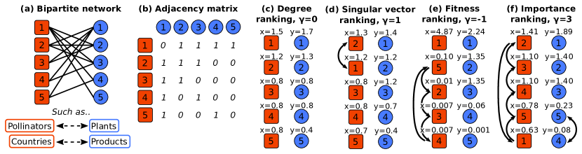
Figure 1: Toy example of a bipartite system, which is represented as a non directed, unweighted, bipartite network, (a), where a set of nodes, e.g. countries or pollinator animals, interact with a disjoint set of other nodes, e.g. products or plants. Such a network is associated with the adjacency matrix (b), in which the element is equal to $1$ if there is a link between the two nodes. The next four panels show the scores and the rankings that Eq. 1 provides for four values of $\gamma$. The black arrows between nodes are changes in the ranking with respect to the degree ranking.

This section presents the non-linear map and how to use it to measure the node importance for bipartite networks. We consider unweighted undirected bipartite networks, with an $N\times M$ adjacency matrix $A$, with $A_{ij}\in\{0,1\}$ (Fig. 1a,b). We denote with $\mathbf{x}$ the scores of the nodes in the first layer of the network, and with $\mathbf{y}$ the scores relative to the second layer. The scores are iteratively updated by the map, which starts from vectors of ones as initial conditions, i.e., $x_{i}^{(0)}=1$ and $y_{j}^{(0)}=1$, and is defined by the equations

$$\left\{\begin{aligned} &x_{i}^{(t)}=\frac{\tilde{x}_{i}^{(t)}}{\langle\tilde{\mathbf{x}}^{(t)}\rangle},\;\text{ where }\;\tilde{x}_{i}^{(t)}=\sum_{j=1}^{M}A_{ij}\left(y_{j}^{(t-1)}\right)^{\gamma},\\ &y_{j}^{(t)}=\frac{\tilde{y}_{j}^{(t)}}{\langle\tilde{\mathbf{y}}^{(t)}\rangle},\;\text{ where }\;\tilde{y}_{j}^{(t)}=\sum_{i=1}^{N}A_{ij}\left(x_{i}^{(t-1)}\right)^{\gamma}.\end{aligned}\right.$$ (1)

The angular brackets denote the vector average $\langle\mathbf{x}\rangle=\sum_{i=1}^{N}x_{i}/N$. The map, possibly, converges to stationary values, which represent the importance measure of the nodes. In general, there is no guarantee that a stationary condition exists. However, we could define a ranking of the nodes from the map behavior at large $t$ for all the empirical systems considered. A detailed discussion about the map convergence is postponed to Sect. III.4.

The numerical approximations that have to be applied to reliably simulate the map and a pseudocode are discussed in the Supplementary Material, Sec. 1. The algorithm, and some of its applications, can be downloaded from the public repository https://github.com/amazzoli/xymap.git.

The map depends on the free parameter $\gamma$ which can be tuned depending on the idea of node importance suggested by the system in analysis. In particular, the generalized map recovers known measures of importance for specific values of $\gamma$, as detailed in the following.

III.1.1 Degree centrality, $\gamma=0$

The simplest case is the degree centrality, which is defined as the number of neighbors of a node, and can be obtained for $\gamma=0$. In this case, the stationary solution is reached at the first map iteration, and the scores are simply the node degree divided by the average degree of the layer. Fig. 1c shows the degree ranking of the toy example illustrated in Fig. 1a.

III.1.2 Singular vector centrality, $\gamma=1$

For $\gamma=1$ the importance of a node is proportional to the importance of the connected nodes in the other layer. In other words, a node is important if it has a lot of important neighbors. The illustrative example in Fig. 1d shows that this notion of importance leads to a different ranking with respect to the case of $\gamma=0$ (i.e., degree centrality). In particular, the second squared node now surpasses the first one in the ranking because, even if it has less connections, it is connected to the most important circular node in the opposite layer.

This is the foundational idea of the eigenvector centrality in classical non-bipartite networks Bonacich (1987). According to this measure, the importance $c_{i}$ of a node $i$ is

$$c_{i}=\lambda^{-1}\sum_{j=1}^{N}B_{ij}c_{j},$$

where $B$ is the $N\times N$ adjacency matrix, which we assume to be symmetric and irreducible, i.e., the network is undirected and connected. The equation above, when written in matrix form, is satisfied by each eigenvector of $B$ with corresponding eigenvalue $\lambda$: $B\mathbf{c}=\lambda\mathbf{c}$. To resolve the ambiguity of having multiple possible choices for the scores, the scores are required to be all positive. This constrains the choice to the eigenvector corresponding to the largest eigenvalue, since the Perron-Frobenius theorem proves that it is the only eigenvector with all positive components  Hogben (2013). Therefore, the leading eigenvector of $B$ defines the so-called eigenvector centrality. This definition of score is arbitrary to within a multiplicative constant. However, one is usually interested in the node ranking, which is not affected by this degree of freedom. An important property of the eigenvector centrality is that it can be computed in a dynamical way, in the similar spirit of the map given by Eq. 1. Starting from a vector of ones as initial condition, the recursive relation $\mathbf{c}^{(t+1)}=\lambda^{-1}B\mathbf{c}^{(t)}$, converges to the leading eigenvector, in the limit of large $t$.

This measure can be extended to bipartite network Daugulis (2012). Since the adjacency matrix $A$ is rectangular in this case, the concept of eigenvector is substituted with left/right singular vectors, and eigenvalue with singular value. Supplementary Material, Sec. 2 shows the proof that the iteration of the Eq. 1 for $\gamma=1$ leads to a vector of scores $\mathbf{x}$ which is proportional to the leading left singular vector $\mathbf{u}_{1}$ of $A$ (corresponding to the largest singular value $\sigma_{1}$), while $\mathbf{y}$ is proportional to the leading right singular vector $\mathbf{v}_{1}$:

$$\begin{aligned} \mathbf{x}&\propto\mathbf{u}_{1}\\ \mathbf{y}&\propto\mathbf{v}_{1}\end{aligned}\hskip 14.22636pt\text{where}\hskip 14.22636pt\begin{aligned} A^{T}\mathbf{u}_{1}=\sigma_{1}\mathbf{v}_{1}\\ A\mathbf{v}_{1}=\sigma_{1}\mathbf{u}_{1}\end{aligned}$$ (2)

Again, the Perron-Frobenius theorem guarantees that the leading singular vectors are positive, and therefore consistent with the unique definition of a positive score.

It is useful to describe one possible example of application of this score system: rating the desirability of products which have been used by a set of consumers Daugulis (2012). This can be described by a consumer-product bipartite system which has links whether a consumer has tried a product. Clearly, the more a product is consumed (high degree) the more important it is, but one can also speculate that an “experienced” consumer increases further the importance of the products that it has tried. The evaluation of consumer experience can be made by the amount of the tried products and if those tried products are considered very desirable. Another important example is the measure of economic complexity introduced in Hidalgo and Hausmann (2009) (with a small difference in the normalization factor of the map).

III.1.3 Fitness-complexity map, $\gamma=-1$

The choice of the exponent $\gamma=-1$ recovers the fitness-complexity map introduced in the context of economics Tacchella et al. (2012); Cristelli et al. (2013, 2015). The score $x_{i}$ corresponds to the fitness, while the score $y_{j}$ is the inverse of the complexity. Therefore, the fitness-complexity map is recovered through the substitution $\tilde{q}_{j}=\tilde{y}_{j}^{-1}$ for every $j$, and defining the complexity as $q_{j}=\tilde{q}_{j}/\langle\tilde{q}\rangle$.

In this regime, the map attributes large importance to nodes with many connections, but, differently from the previous case of $\gamma=1$, the connections with low-importance neighbors have a larger weight. This effect is shown by the ranking in Fig. 1e, where the squared node $5$ increases its position in the ranking with respect to the degree sorting, and surpasses the higher-degree node $2$. Indeed, node $5$ is connected to the circular node $4$, which has the second lowest importance, while the squared nodes $2$, $3$, and $4$, are not.

The fitness-complexity map was introduced to quantify the non-monetary competitiveness of a country on the basis of its exported products. The basic idea is that the fitness (i.e, the $x$ score) of a country is proportional to the sum of the complexities of its exported products, which in our notation is the sum of the inverse of the “simplicities”, given by the $y$ scores. The simplicity of a product is large if many countries can export that product, in particular if these countries have low fitness. On the contrary, a product is complex ( i.e., low $y$) if only few countries with high fitness can produce it.

The range of application of the fitness-complexity map extends to other bipartite networks. For example, it has been used to analyze the contribution of different countries to a set of scientific topics  Cimini et al. (2014). A different field of application are mutualistic ecological networks. In the case of the interactions between plants and pollinators, the fitness of an animal pollinator seems to be significantly related to its ecological importance within the ecosystem, while the complexity of a plant quantifies its vulnerability to system perturbations Domínguez-García and Muñoz (2015). This ecological example will be our main illustrative application.

III.1.4 Behavior at large exponents

It is instructive to characterize the map behavior for large exponents. In the case of $\gamma\gg 1$, the first score of Eq. 1 can be approximated as:

$$x_{i}^{(t)}\propto\frac{\max_{j\in J(i)}\left(y_{j}^{(t-1)}\right)^{\gamma}}{\max_{j\in\{1,\ldots,N\}}\left(y_{j}^{(t-1)}\right)^{\gamma}},$$ (3)

where the maximum at numerator comes from the approximation of $\tilde{x}^{(t)}$, and it is evaluated among the set $J(i)$ of neighbors of $i$. The maximum at denominator is instead the leading term of $\langle\tilde{x}^{(t)}\rangle$, and considers the largest y-score among all the nodes of the second layer. This expression implies that only the nodes connected with the maximal y-score have non-negligible x-score and, therefore, will dominate the ranking. In this limit, the degree of the node does not enter explicitly in the computation. This can be seen in Fig. 1f, which displays a ranking calculated for $\gamma=3$. The squared node $1$, which is the most connected among the squared nodes, becomes the last one in the ranking, since it lacks the connection with the most important circular node, i.e., the first one. The opposite limit of $\gamma\rightarrow-\infty$ leads exactly to the same result of Eq. 3, but with a minimum instead of a maximum. Therefore, the $x$-score is determined by the connection with the minimal $y$-score.

III.1.5 General intuition behind the map behavior

Putting all these considerations together one can conclude that the absolute value of $\gamma$ sets the balance between two properties in determining the importance of a node. The first is the degree of the node which, for $\gamma=0$, is the only relevant feature. The second property is the connection with important nodes in the other layer: in the limit of large $|\gamma|$, only the maximum (or minimum) score among the connected neighbors contributes to the importance. The sign of $\gamma$ determines if the importance is given by having high-score neighbors (positive $\gamma$) or low-score ones (negative $\gamma$).

III.2 Looking for the specie ranking which maximizes the extinction area

We can now evaluate the ranking generated by the map on ecological systems of mutualistic interactions between species, such as plants and pollinators. We use the extinction area to quantitatively evaluate the goodness of the rankings Domínguez-García and Muñoz (2015); Allesina and Pascual (2009). The computation of this quantity is illustrated in Fig. 2a-c. Given an animal ranking (e.g., $(A_{1},A_{2},A_{3})$), we can first remove the first animal ($A_{1}$) and all its links. As a consequence, a certain number of plants remain without links and thus get extinct ($F_{1}$ in the example).

By progressively removing all the animals according to the ranking, we can calculate the fraction of extinct plants as a function of the fraction of removed animals (Fig. 2c). The extinction area is defined as the integral of this curve, and quantifies the speed of the ecosystem collapse for the given ranking.

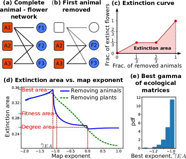
Figure 2: The panel (a), (b) and (c) show a toy example of the extinction area computation. Starting from the complete network (a), animals are removed according to a certain ranking. In (b) the animal $A_{1}$ has been deleted leading to the extinction of the flower $F_{1}$ which remains without links. The extinction area is the integral of the curve (c) which shows the fraction of extinct flowers at a given fraction of removed animals. The panel (d) is the extinction area for different map exponents $\gamma$ of the mutualistic system Robertson 1929. The blue continuous line is the area computed in the same way of the toy example above, where the animal ranking is provided by the $x$-score at the given $\gamma$. The green dash-dot line is computed using the opposite procedure: the plants are removed following the $y$ ranking keeping track of the extinct animals. The right-bottom panel shows the distribution of the map exponent at which the area is maximized removing rows, $\gamma_{EA}$, among $116$ mutualistic networks of the Web-of-Life database, see II, having size (product between the number of rows and columns) larger that $500$.

A previous work Domínguez-García and Muñoz (2015) demonstrated that the fitness-complexity map, that we recover for $\gamma=-1$, provides an animal ordering that leads to a larger extinction area than other algorithms. Fig. 2d shows that, in a specific case, our map can reach even larger values of extinction area for other values of $\gamma$. In particular, there is a maximum at $\gamma_{EA}\simeq-1.12$. The improvement with respect to the fitness-complexity map is even larger than the improvement that the fitness-complexity map has compared to the simple degree ranking ($\gamma=0$).

The value of $\gamma$ that maximizes the area, $\gamma_{EA}$, is dataset dependent. We notice that in all the cases we studied the optimal value of $\gamma$ was strictly smaller than -1 and typically within the range $\gamma_{EA}\sim[-1.4,-1]$. We report in Fig. 2 the distribution of the best parameters for all the mutualistic networks discussed in section II. We shall further discuss the issue of finding the best gamma and, in particular, the origin of the $\gamma_{EA}<-1$ bound in the next section (Eq. 7).

One further question is how close the obtained extinction area is to the global maximum. We can explore a large population of rankings by employing a genetic algorithm that searches for the best extinction area. Supplementary Material, Sec. 3 shows that, for different ensembles of randomly generated matrices, the average best extinction area found by our map always coincides or is better than the genetic-algorithm result. It is worth noticing that the iterative map is typically 100 times faster than a genetic algorithm, as also discussed in Supplementary Material, Sec. 3.

III.3 Looking for the species ranking that maximizes the matrix nestedness

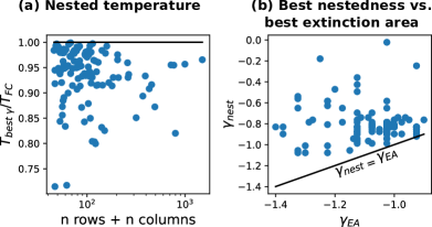
Figure 3: (a): ratio of the nestedness temperature between the fitness-complexity map, $\gamma=-1$, $T_{FC}$, and the best temperature found by our algorithm, $T_{best\;\gamma}$. Each point is an ecological matrix of Sect. II. On the x-axis we show the matrix size as the sum of the number of rows and columns. (b): for each matrix we plot the value of $\gamma$ that maximizes the extinction area, y-axis, and the one that maximized the nestedness temperature, x-axis.

The classical way to measure the nestedness of a network depends on the reordering of rows and columns Atmar and Patterson (1993). Given a row and column order, one can compute a nestedness temperature and the final temperature of the network is the maximal one among all the possible orders. Therefore, this measure relies on algorithms that have to explore the factorially growing space of possible rankings of rows and columns.

The fitness-complexity map has been shown to be very efficient for this purpose, finding rankings that perform better than state-of-art search algorithms in several cases Lin et al. (2018). This task can be tackled with our map by varying the parameter $\gamma$ and choosing the value minimizing the nestedness temperature as defined in reference Rodríguez-Gironés and Santamaría (2006)). The temperatures that we find are typically better than the ones at $\gamma=-1$ ( Fig. 3a). In particular, we find lower temperatures also for larger matrices, where the fitness-complexity map was performing slightly worse than the state of the art, as reported in Fig. 3 of reference Lin et al. (2018). Interestingly, the best parameters for this task, $\gamma_{nest}$, take values in the range $[-1,0]$. Fig. 3b shows the scatter plot of this value and the one that maximizes the extinction area for the same matrix. One would naively expect that these two tasks are somehow similar, since they both try to “triangularize” the adjacency matrix. However, the exponents for the two tasks take values in different regions of the parameter space, i.e., before and after $\gamma=-1$. Moreover, the values are are not correlated (Spearman $\rho=0.01$, $\text{p-val}=0.9$).

III.4 A phase transition suggests the value of $\gamma$ maximizing the extinction area

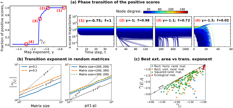
Figure 4: The panel (a) shows the transition of the fraction of scores which converge to positive values of the plant-pollinator matrix Robertson 1929 (see Sect. II). The four red circles above the blue line of the plot on the left are associated to the four plots on the right, which show the $x$-score trajectories for different exponents. The line colors refer to the node degree. The panel (b) displays the absolute value of the transition exponent, $\gamma_{c}$, for the $x$-score as a function of the size and the density in uniform random matrices. Each point is computed as an average over $5$ matrices generated with the same parameters. The panel (c) shows the scatter plot of the exponent which maximizes the extinction area, $\gamma_{EA}$ and the exponent of the phase transition, $\gamma_{c}$, for uniform random matrices and the $20$ largest ecological matrices (red points). The other three colors are different shapes of uniform random matrices: horizontal $N=s/1.5,M=s*1.5$, vertical $N=s*1.5,M=s/1.5$, and squared $N=M=s$. The considered matrices have been generated with different sizes $s$, between $50$ and $200$, and different densities between $0.2$ and $0.4$.

This section examines on the stationary behavior of the general map described by Eq. 1 for different values of $\gamma$. For the convergence analysis as a function of the input matrix in the specific case of $\gamma=-1$, please refer to ref. Pugliese et al. (2016).

As the number of iterations of the map increases, the scores $x_{i}$ and $y_{j}$ tend to an asymptotic behavior which strongly depends on the value of $\gamma$. For special choices of the adjacency matrix and of $\gamma$, this limiting behavior may even be an oscillatory type. However, the generic situation is that the scores tend well defined and finite fixed points. We observe that the fixed points are all strictly positive for positive parameters ($\gamma>0$), as well as for negative and small parameters, i.e., $\gamma<0$ and $|\gamma|\ll 1$. An example is reported in Fig. 4a1). On the other hand, for small enough values of $\gamma$, some of the scores can tend to zero as in the examples of panels Fig. 4a2-4. This latter phenomenology could create an ambiguity in the ranking definition. However, not all the nodes’ scores tend to zero with the same speed, and we can thus rank first the nodes that have a slower score decay, as better explained in Supplementary Material, Sec. 1.

Interestingly, how the fraction of zero-scores changes as a function of $\gamma$ strongly resembles a phase transition. This is displayed in Fig. 4a1 for the particular case of the Robertson 1929 matrix. For exponents close to zero, the score is proportional to the node degree, implying that all the fixed points are positive: $f=1$. Also when the exponent is decreased from zero to values near $-1$, for instance at $\gamma=-0.75$ in Fig. 4a1, all the scores reach positive values. Approaching $\gamma=-1$, a small fraction of trajectories begins decaying to zero, as in Fig. 4a2. Moving from $-1$ towards a “critical” exponent, the fraction of positive trajectories decreases, as shown in Fig. 4a3, for $\gamma=-1.1$. Finally, after a discontinuous transition, there is a ”condensation phenomenon” with most trajectories converging to zero with few exceptions, as in Fig. 4a4 for $\gamma=-1.3$. As it typically happens in phase-transition phenomena, the time required for convergence increases approaching the transition. This abrupt transition from a macroscopic number of positive scores to a fraction of order $1/N$ is present across all the different empirical cases we have considered (see Supplementary Material, Sec. 4).

Moreover, the behavior of the order parameter as a function of $\gamma$ in the case of random interaction matrices $A_{i,j}$ shows that the its jump becomes steeper with the matrix size. This is exactly the expected phenomenology for a phase transition in the thermodynamic limit, i.e., in the large matrix size limit. This allows to define a critical value $\gamma_{c}$ which in the thermodynamic limit separates the $f\sim 1$ phase (for $\gamma>\gamma_{c}$) from the $f\sim 0$ phase (for $\gamma<\gamma_{c}$). In the empirical cases, this critical value is rounded out due to the finite size of the interaction matrix, as it can be seen in Fig. 4. However, despite finite size effects, the critical $\gamma$ region is narrow and transition in the order parameter still evident.

Even if the underlying dynamics is different, this phase transition strongly resembles the condensation phenomena discussed for instance in Godrèche (2019) or in Bianconi and Barabasi (2001). The score of one (or few) node takes a macroscopic value and the other scores ones are pushed to zero due to the normalization constraint. For this reason, we denote the $f=0$ phase for $\gamma<\gamma_{c}$ as the “condensed phase” and the $\gamma_{c}$ as the “condensation point”.

Unfortunately, there is no obvious way to predict the value of $\gamma_{c}$ for a given empirical interaction matrix. However, the calculation of Supplementary Material, Sec. 5 derives an upper bound in the limit of large matrices:

$$\gamma_{c}\leq-1$$ (4)

III.4.1 Phase transition in uniform random matrices

In the case of uniform random matrices, the scaling of the critical map-exponent with the parameters of the adjacency matrix can be understood with the following computation. Let us choose the matrix elements to be Bernoulli random variables, such that $A_{ij}=1$ with probability $p$ and $A_{ij}=0$ with $1-p$, where the matrix has size $(N,M)$. The map starts from initial conditions of ones, $x_{i}^{(0)}=1$ and $y_{j}^{(0)}=1$, and, after one step, it leads to sums of independent and identically distributed random variables: $\tilde{x}^{(1)}_{i}=\sum_{j=1}^{M}A_{ij}$. Using the central limit theorem one can obtain the following expressions:

$$\begin{cases}{x}^{(1)}_{i}=1+\sqrt{\frac{1-p}{Mp}}\eta\\ {y}^{(1)}_{j}=1+\sqrt{\frac{1-p}{Np}}\eta,\end{cases}$$ (5)

where $\eta$ is the standard normal random variable ($\langle\eta\rangle=0$ and $\text{Var}(\eta)=1$). At the next step the non-normalized score reads:

$$\tilde{x}^{(2)}_{i}=\sum_{i}^{M}A_{ij}\left(1+\sqrt{\frac{1-p}{Np}}\eta\right)^{\gamma}.$$

If $|\gamma|$ is small, the score can be approximated at first order in the following small quantity: $|\gamma|\sqrt{(1-p)/(\min({N,M})p)}\ll 1$. This leads to a summation of variables, both for $x^{(2)}$ and $y^{(2)}$, which have the same first and second moment of the Bernoulli matrix element. As a consequence, by applying again the central limit theorem, the score at the second step has the same distribution of the score at the first step (Eq. 5), implying that the stationary solution has been reached. The scores follow a Gaussian distribution, and are all positive. Thus for these values of $\gamma$ the system is in the $f=1$ phase. We know that for large enough negative values of $\gamma$ this solution is certainly unstable and the system is in the condensed phase. If we assume that the onset of the condensed phase coincides with the values of $\gamma$ for which the above approximation is not any more valid. i.e. $|\gamma|\sqrt{(1-p)/(\min({N,M})p)}=O(1)$, we can derive the following scaling relationships for the critical exponent:

$$\gamma_{c}\sim-\sqrt{\frac{\min({N,M})p}{1-p}}.$$ (6)

Those predictions are verified in Fig. 4b.

III.4.2 The connection between condensation and the best extinction area

The condensation of a few scores to positive values seems to be related to the good performance in finding the extinction area. This is shown by Fig. 4c, where the transition exponent, computed according to the procedure described in Supplementary Material, Sec. 4, is plotted as a function of the exponent that maximizes the extinction area $\gamma_{EA}$. Combining this this empirical observation with Eq. 4, we can derive the following bound:

$$\gamma_{EA}\leq\gamma_{c}\leq-1.$$ (7)

III.5 The condensation implies a triangular shape of the adjacency matrix

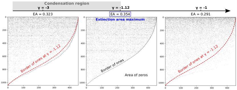
Figure 5: Examples of matrices with rows and columns sorted according to the $x$ and $y$ ranking for three different map exponents, $\gamma=-3,-1.12,-1$, of the same mutualistic system (Robertson 1292 matrix). A black dot corresponds to the entry $1$, while a white dot to the entry $0$. $\gamma\simeq-1.12$ is the value which maximizes the extinction area, as shown in Fig. 2d. The exponents less or equal than $-1.12$ are in the condensation phase, see Fig. 4a, and present the typical border of ones that separates a right-bottom area of zeros from the rest of the matrix.

The shape of the adjacency matrix, when ordered according to the map ranking, shows a clear geometric pattern in the condensation phase. Fig. 5 shows the matrix corresponding to an ecological example (Robertson 1929), with the ones represented in black and the zero entries in white. Three different rankings are displayed corresponding to three different value of the exponent $\gamma$. In the condensed phase, a large area of contiguous zeros appears in the bottom right corner. The area is well separated by the top left area by a continuous border of ones. The calculation of Supplementary Material, Sec. 5 shows how both these features can be derived from the map (Eq. 1) with the only assumptions of having the system in the $f=0$ condensed phase, and the solution to be stable.

There is a connection between this packing phenomenology and the extinction area. Supplementary Material, Sec. 6 proves that the extinction area obtained by removing the rows is a linear function of the area of consecutive zeros from the matrix bottom. Specifically, if we define $z_{j}$ as the number of consecutive zeros from the matrix bottom of the column $j$, and $Z=\sum_{1}^{M}z_{j}$ the total area of zeros, the extinction area obtained removing rows, $E$, reads:

$$E=\frac{1}{N}\left(\frac{Z}{M}+1\right),$$ (8)

where $N$ and $M$ are the number of rows and columns respectively. A similar relation can be derived also for the transposed quantities. In other worsds, the extinction area obtained by removing columns is linearly dependent on the area of zeros from the matrix right. These relations connect the extinction area with the visual triangular pattern of the adjacency matrix, and we expect that the ordering with the largest area of zeros (second matrix of Fig. 5) would also have the largest extinction area.

The results of the last two sections suggest that the behavior of the map in the condensed phase drives the ranking of nodes in a way that it “triangularizes” the adjacency matrix, leading to a large area of zeros of the bottom right corner, which also implies a large (almost optimal) extinction area. It is important to stress that we are only able to prove that the triangular shape is a consequence of the condensation and that the extinction area is closely connected with this area of zeros. However, we do not have analytical results about the optimality of the extinction area. As a general empirical fact, in all the studied cases the best extinction area is always reached in the condensation phase and close to the transition point, and therefore for $\gamma<-1$.

IV Discussion

Bipartite networks are the natural description for various complex systems in technological Pang and Maslov (2013); Mazzolini et al. (2018b), social Vasques Filho and O’Neale (2020); Koskinen and Edling (2012), economical Hidalgo and Hausmann (2009); Cristelli et al. (2013), linguistic Gerlach et al. (2018b), and biological Corel et al. (2018); Mazzolini et al. (2018a) domains. We introduce a tool to rank nodes in bipartite networks according to different concepts of importance. The scores used for ranking are defined through a non-linear map connecting the two network layers. The map depends on the network adjacency matrix and on an exponent $\gamma$ which dictates the non-linearity, and implicitly defines node importance. By adjusting $\gamma$, users can tailor the analysis to the specific task and incorporate prior beliefs about node relevance. In particular, we have shown how specific $\gamma$ values correspond to well known definitions of node importance. More generally, given a metric to measure how good a ranking is, we can look for the optimal $\gamma$ value. For instance, we examined the problem of identifying the optimal extinction area in ecological interaction matrices and the ranking that maximizes their nestedness temperature. These tasks have been previously effectively addressed using the fitness-complexity map, which correspond to $\gamma=-1$ in our framework Domínguez-García and Muñoz (2015); Lin et al. (2018). Our results indicate that the optimal $\gamma$ values range from $[-1.4,-1]$ for the extinction area, and from $[-1,0]$ for nestedness. The optimal values vary based on the specific task and dataset, making them challenging to predict in advance. However, theory can help in limiting the range of parameters that should be explored. For example, we could analytically set the upper bound at $\gamma_{EA}=-1$ for the extinction area, Eq. 7. Our theoretical argument is based on the presence of a dynamical phase transition for large enough negative values of $\gamma$. This transition separates the score space into two phases. For $\gamma>\gamma_{c}$ all scores remain finite and positive, whereas for $\gamma<\gamma_{c}$ a “condensed” phase emerges where only one or few scores dominate, pushing the others towards zero through normalization. We first established an upper bound for this transition as $\gamma_{c}\leq 1$, and then we postulated (and check numerically, Fig. 4) that the extinction area is maximized in the condensed phase, $\gamma_{EA}\leq\gamma_{c}$. This picture is coherent with the visual inspection of the adjacency matrix ordered according to the ranking in the condensed phase. We proved that the extinction area is proportional to the area of consecutive zeros from the bottom-right of the matrix and, indeed, the matrix takes a clear triangular shape, with a border of ones separating a “large” bottom-right area of zeros.

Although we focused on ecological systems, it would be valuable to explore the applicability of our generalized map in other fields. For instance, several results have been obtained using the fitness-complexity algorithm (i.e., the $\gamma=-1$ case) in economic systems Tacchella et al. (2012); Cristelli et al. (2013, 2015); Servedio et al. (2018); Tacchella et al. (2018). In particular, there is an interesting ongoing debate on the meaning and the evaluation of the “complexity” of exported products and on the “fitness” of the exporter nations Morrison et al. (2017); Sciarra et al. (2020); Balland et al. (2022). Different economic definitions would ideally correspond to different values of $\gamma$ and can thus lead to different rankings of nations.

Besides its practical applications, our non-linear map represents a relatively simple model with a rich phenomenology and an emergent ”dynamical” phase transition that could be explored in more depth with statistical physics tools. For example, understanding the deep connection between the condensation phase transition and the maximum of the extinction area, shown by Fig. 4c, is still an open issue. These two features seem closely connected by the triangular shape of the adjacency matrix. However the actual proof that the condensation is necessary for the maximal extinction area (or the maximal that our mapping can provide) is still missing. The possible connection between the condensation we observe and the well studied condensation transition in network theory is also an open problem Bianconi and Barabasi (2001).

Our framework represents only one possible generalization of ranking algorithms based on non-linear maps as the fitness-complexity map Tacchella et al. (2012). A previous attempt along this line Mariani et al. (2015) can actually be easily included in our framework by re-defining the exponents for the $x$ and $y$ layers, i.e., $\gamma_{x}=-\beta$ and $\gamma_{y}=-1/\beta$. However, our symmetric choice in Eq. 1 is computationally more efficient and leads, for example, to larger extinction areas as analyzed in more detail in Supplementary Material, Sec. 7.

A more general extension of our map, which we plan to investigate, involves a two-parameter version where the non-linearity differs between the two layers, i.e., $\gamma_{x}\neq\gamma_{y}$. In this case, the $\gamma_{x},\gamma_{y}$ plane could be explored to select the best combination of exponents given the task at hand. This generalization would allow the introduction of different principles of node importance on the two layers with the consequent coupled rankings. The statistical properties of this more general map in terms of convergence and phase transitions could present an even richer phenomenology.

Finally, our approach can also be extended to study node centrality on large multiplex networks Battiston et al. (2017); Rahmede et al. (2018). Multiplex networks are playing an increasingly important role in modern big data analyses. Many of these networks could be represented as multi-partite networks and could thus be approached with an extension of our map. Moreover, multiplex networks implicitly have a natural bipartite scheme with the nodes on one side and the layers of the multiplex on the other side. Weighted links connect a node with a layer with a weight proportional to the number (and centrality) of neighboring nodes present in that layer. Following Rahmede et al. (2018), we may rank the importance of nodes by increasing the centrality of nodes that receive links from highly influential layers, and symmetrically enhance the influence of a layer if it contains central nodes. This idea naturally leads to an iterative map, but extended to include a weighted adjacency matrix. An additional non-trivial extension of our approach could be developed for temporal networks Holme and Saramäki (2012), adding yet another layer of dynamics to the non-linear map.

SUPPLEMENTARY MATERIAL

S1 Computational issues

The $x$/$y$-scores are provided by the dynamical iteration of the map (1) of the main text. In this section we discuss some technical points and approximations that are necessary to carry out a reliable numerical simulation of it.

S1.1 Dealing with the zeros

A straightforward simulation of the $x$-$y$ map has the problem that some of the scores can have zero as fixed point. If $\gamma<0$, those scores have to be elevated to a negative power, implying that some approximations must be introduced to deal with infinite values. To understand the correct way to keep into account those zeros, let us go through the simple example of Figure S1.

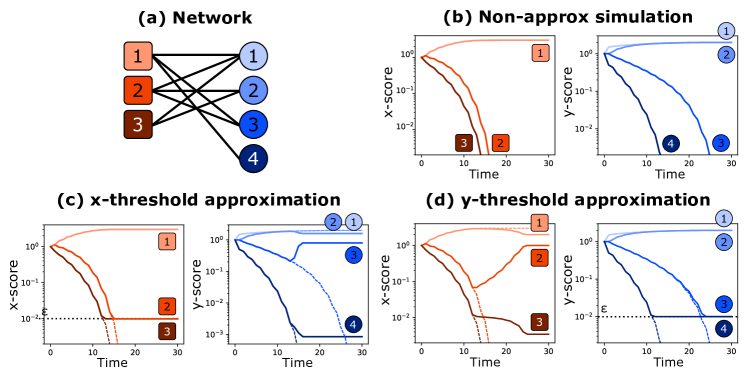
Supplementary Figure S1: Trajectories of the $x$ and $y$ scores for the network in panel (a), evaluated with the algorithm at $\gamma=-1.2$. Panel (b) shows the non-approximated algorithm, panel (c) the map with a threshold $\epsilon$ imposed on the $y$ score, while panel (d) on the $x$ score. In panel (c) and (d) the dashed lines are to the non-approximated trajectories.

The trajectories for a negative $\gamma$ without any approximation is shown in panel (b). Note that we can run the map without approximation only because the system is small and the simulation runs for a few time steps. This shows one positive fixed point and two zeros for the $x$-scores, while two positive and two zeros for the other layer. In general, the trajectories that go to zero will eventually reach the numerical limit and they will be approximated with a zero, leading to a division by zero. One possible solution is that, once a trajectory reaches a small value $\epsilon$, it stops decaying and it is set equal to $\epsilon$ for all the remaining time. Panel (c) shows this procedure for a threshold $\epsilon$ applied only to the $x$-scores: $x_{i}\rightarrow\max\{x_{i},\epsilon\}$. The $y$-scores are computed without approximations. Looking at the panel, it seems that $x$ scores follow the true trajectories (represented by dashed lines) until the threshold is reached. In that case, the ranking can be computed putting the scores that reach the threshold first at lower positions in the ranking. However, the $y$ scores show a weird behavior, and, in particular, the node number $3$ converges to a positive value, while the panel (b) says that it should go to zero. In panel (d) the threshold is imposed to the $y$ scores, showing a reliable approximation for the $y$s, but not for the $x$s. This picture does not change for the more complex case of Figure S2a, which shows the good approximation of $x$-thresholding for the $x$-scores, while an unreliable set of trajectories for the $y$ scores (with changes in the ranking with respect the true computation), and similarly for $y$-thresholding in panel S2b.

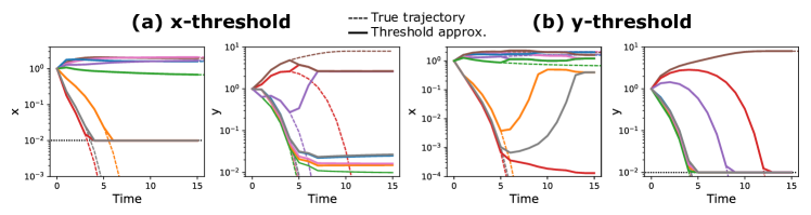
Supplementary Figure S2: Threshold approximation for a $8\times 8$ matrix. The $x$-scores for the $x$-thresholding and the $y$-scores for the $y$-thresholding overlap almost perfectly the non-approximated trajectories (dashed lines).

S1.1.1 Wrong approximation of the $y$-score by the $x$-thresholding

To better understand this behavior, let us first focus on why the $x$-threshold approximation does not work well for the $y$ score. The same reasoning can be transposed to the $y$-threshold. For example, we can focus on the $y$-trajectory of node $3$ in panel S1c. This trajectory should go to zero, as panel (b) shows. Indeed, in the regime where $x_{1}\simeq 3\gg x_{2}\gg x_{3}$ (reached after few time steps), the score at the next step $y_{3}^{\prime}$ as a function of the score two steps before $y_{3}$, reads:

$$y_{3}^{\prime}=\frac{x_{1}^{\gamma}+x_{2}^{\gamma}}{\frac{1}{3}(3x_{1}^{\gamma}+3x_{2}^{\gamma}+2x_{3}^{\gamma})}\simeq 2\left(\frac{x_{2}}{x_{3}}\right)^{\gamma}\simeq 2\left(\frac{y_{3}}{2}\right)^{\gamma^{2}}\propto y_{3}^{\gamma^{2}}$$

where the third equality is obtained by using the expression of the $x$-scores as a function of the previous $y$-scores, and assuming $y_{1}=y_{2}=2\gg y_{3}\gg y_{4}$. Since $y_{3}$ is smaller than $1$ and $\gamma^{2}$ is a positive exponent, the trajectory will decay (more than exponentially) to zero. This corresponds to the correct behavior, however when both $x_{3}$ and $x_{2}$ hit the threshold $\epsilon$ ($x_{1}=3\gg x_{2}=x_{3}=\epsilon$), the value of $y_{3}^{\prime}$ becomes constant and equal to $y_{3}=4/5$, drastically changing the fixed point value. Also the two larger scores $y_{1},y_{2}$ deviate from the true fixed point $2$ and converge to $8/5$.

In general, the thresholding procedure affects the smallest $x$-scores, but, for $\gamma<0$, the smallest $x$-scores are also the most important contributions in computing the $y$-scores (the largest $y$s are the ones connected with the smallest $x$s). In the next section it is shown that, quite surprisingly, even though these scores are wrong, the $x$-scores computed with the $x$-thresholding are instead well approximated.

S1.1.2 Good approximation of the $x$-score by the $x$-thresolding

Let us write down the trajectories of the non-approximated $x$s in the regime $x_{1}\simeq 3\gg x_{2}\gg x_{3}$:

$$\begin{cases}x_{1}^{\prime}\simeq 3\\ x_{2}^{\prime}\simeq 3\left(\frac{x_{2}}{3}\right)^{\gamma^{2}}\\ x_{3}^{\prime}\simeq 3\;2^{\gamma}\left(\frac{x_{3}}{3}\right)^{\gamma^{2}}\end{cases}$$ (S1)

Where, the score $x_{i}^{\prime}$ is expressed as a function of the score two steps before, $x_{i}$, using the map two consecutive times: the first to compute the $y$s as a function of the $x$s, and the second to get $x_{i}^{\prime}$ as a function of the $y$s. Considering Figure S1b, this behavior is followed until $x_{3}$ hits the threshold, let us say, at time $t_{1}$. For $t>t_{1}$ this score is then imposed to be $x_{3}=\epsilon$. We also define $t_{2}$ as the time at which the trajectory $x_{2}$ becomes smaller than $\epsilon$ and it is set equal to $\epsilon$. Between $t_{1}$ and $t_{2}$ the trajectories can be computed applying the map two times as before, but having $x_{3}=\epsilon\ll 1$ and the condition $x_{2}\gg x_{3}$ no longer satisfied. The result is:

$$\begin{cases}x_{1}^{\prime}\simeq 3\\ x_{2}^{\prime}\simeq\frac{3}{3^{\gamma^{2}}}\left(2(x_{2}^{\gamma}+\epsilon^{\gamma})^{\gamma}+x_{2}^{\gamma^{2}}\right)\\ x_{3}^{\prime}=\epsilon\end{cases}$$ (S2)

Therefore, the largest score is not affected at all, while $x_{2}$ changes its trajectory. However this change is negligible as long as it stays away from the threshold $x_{2}\gg\epsilon$ (the equation above for the correct behavior can be easily recovered in this regime). When $t>t_{2}$, and $x_{2}=x_{3}=\epsilon$, one can see that the map provides again the right value for $x_{1}\simeq 3$. As a conclusion, the trajectories are well approximated as long as the scores are larger than the threshold. The fact that the approximation for the $x$s is good even though the $y$s used to compute them are wrong (as shown in the previous section) can be explained as follows. The threshold imposed to $x_{3}$ changes significantly the values of $y_{1}$ and $y_{2}$ at which it is connected, as we saw before. However, the behavior of $x_{2}$ is dominated by $y_{3}$ ($y_{3}^{\gamma}$ is the largest term in its summation), while $x_{1}$ is driven by $y_{4}$. The scores $y_{1}$, $y_{2}$ affect significantly only $x_{3}$, which has already reached $\epsilon$. As a consequence, the error in $y_{1}$, $y_{2}$ does not “propagates” to the $x$-scores that are larger than the threshold. Similarly, when $x_{2}$ hits the threshold, $y_{3}$ is now affected, but $x_{1}$ depends mostly on $y_{4}$. This can seem a lucky case, but in fact this is due to the structure of the ordered adjacency matrix when there are zeros as fixed points discussed in section S5. Referring to the Figure S5 positions, the first set of nodes that hit the threshold is $\mathcal{N}_{k}$. This strongly affects the values of the $y$-scores of $\mathcal{M}_{0}$ which are the only ones connected to them. However, because of the matrix structure, all the other nodes not in $\mathcal{N}_{k}$ are connected to nodes with smaller $y$ (belonging to $\mathcal{M}_{j>0}$), and therefore the contribution of the wrong estimates is then negligible for the computation of the scores in $\mathcal{N}_{i<k}$. This reasoning can then be applied iteratively for $\mathcal{N}_{k-1}$ hitting the threshold and modifying the $y$-scores in $\mathcal{M}_{1}$. As before, all the nodes in $\mathcal{N}_{i>k-1}$ have at least a connection with a node in $\mathcal{M}_{j>1}$ and the error does not propagate.

In conclusion, imposing a threshold to one of the two layers allows us to carry out a reliable simulation of the scores of that layer. The scores of the other layer have to be obtained with an independent simulation with the suitable thresholding procedure.

S1.2 Convergence criterion

Another important point is to identify the stationary condition, at which the map iteration stops, and the scores are obtained. The following simple procedure for $x$ is employed (and similarly for $y$): at each computational time step, the average differential of the fitness trajectories is computed, and reads as follows:

$$\langle d_{x}\rangle_{t}=\frac{1}{n}\sum_{i=1}^{n}\mid x_{i}^{(t)}-x_{i}^{(t-2)}\mid$$ (S3)

where $t$ is the map time-step. Note that we are using the difference with the scores in $t$ and two steps before. This is because computing the $x$-score every two steps results in a much faster simulation. See the section S1.4 for a pseudocode of the algorithm. The map stops if one of the two following conditions are satisfied: $\langle d_{x}\rangle_{t}<\theta$, where the threshold is chosen equal to $10^{-6}$, or if the number of iterations exceeds a limit value (about $2000$ iterations). The latter condition is required in particular rare cases where the relaxation time becomes extremely large, such as if there are power law decaying trajectories, or when a stationary state does not exists.

S1.3 Computing the ranking

A third crucial point is the ranking computation, i.e. the ordering of the nodes based on the map score. In a scenario where all the score trajectories converge to non-zero values, the ranking can be computed trivially, and it is just given by the sorted scores. However, the presence of trajectories which decay to zero is very common. Clearly these nodes cannot be compared on the basis of their stationary value, which is zero (actually $\epsilon$) for all of them. In such cases, we distinguish between the nodes with non-zero stationary fitness, and the nodes with trajectories decaying to zero and hitting the threshold $\epsilon$. The nodes in the first group are put at the top positions of the ranking, and they are ordered according to their stationary score. The zero trajectories are ranked according to the time at which they went below the boundary. Specifically, the ones that crossed the threshold before are put at lower positions in the ranking.

S1.4 Pseudocode

The following pseudocode is based on the arguments discussed above. An implementation in python of the algorithm can be found at the following repository: https://github.com/amazzoli/xymap.git. Note that instead of using $x$ and $y$, we refer to $a$ as the score that we want to reliably compute, and $b$ the opposite score (that can be affected by the thresholding approximation).

Input: $A$, adjacency matrix of the bipartite network.

Input: $\gamma$, exponent of the map.

Input: $a\in\{x,y\}$, which scores to compute (axis).

Define: $b$, opposite score of $a$, $b=y$ if $a=x$, or $b=x$ if $a=y$.

Input: $\tau_{max}$, maximum number of allowed iterations.

Input: $\epsilon$, zero threshold for approximating the zeros of the $a$-score.

Input: $\delta$, average $a$-score differential below which the algorithm converges.

Initialize: $\mathbf{a}^{(0)}$, $\mathbf{b}^{(0)}$, initial conditions of the scores as vectors of ones.

Initialize: $\mathbf{r}_{a}$, the ranking of the score $a$ as an empty vector.

Initialize: $\mathcal{Z}_{a}$, the set of nodes of the layer $a$ which have reached the threshold $\epsilon$ as an empty set.

Loop: for $\tau=1,\ldots,\tau_{max}$:

$|\;$ Compute the opposite score: $\mathbf{b}^{(2\tau-1)}=A^{T}(\mathbf{a}^{(2\tau-2)})^{\gamma}$

$|\;$ Compute the main score: $\mathbf{a}^{(2\tau)}=A(\mathbf{b}^{(2\tau-2)})^{\gamma}$

$|\;$ Check which nodes have crossed the threshold in this step: $\mathcal{Z}_{a}^{\text{new}}=\{i\;|\;\mathbf{a}^{(2\tau)}_{i}\leq\epsilon\text{ and }i\not\in\mathcal{Z}_{a}\}$.

$|\;$ Update the ranking with the new nodes below threshold: $\mathbf{r}_{a}\leftarrow(argsort[\mathbf{a}^{(2\tau)}_{i\in\mathcal{Z}_{a}^{\text{new}}}],\mathbf{r}_{a})$

$|\;$ Update the set of nodes below threshold $\mathcal{Z}_{a}\leftarrow\mathcal{Z}_{a}\;\bigcup\;\mathcal{Z}_{a}^{\text{new}}$

$|\;$ Impose the threshold approximation: $a_{i}^{(2\tau)}=\epsilon$ if $i\in\mathcal{Z}_{a}$.

$|\;$ Compute the quantity in equation (S3): $\langle d_{a}\rangle$

$|\;$ Check the convergence: If $\langle d_{a}\rangle<\delta$:

$|\;$      $|\;$ Break the loop

Loop end.

Compute the ranking of the nodes with positive fixed point: $\mathbf{r}_{a}\leftarrow(argsort[\mathbf{a}^{(2\tau)}_{i\not\in\mathcal{Z}_{a}}],\mathbf{r}_{a})$

We refer to $t$ as the time of the map written in equation (1) of the main text. $\tau$ is instead the time step of the loop which corresponds to $\tau=\text{int}(t/2)$. Note that the algorithm computes the trajectories every two steps: $(\mathbf{a}^{2},\mathbf{a}^{4},\ldots)$ and $(\mathbf{b}^{1},\mathbf{b}^{3},\ldots)$.

S2 Derivation of the singular vector centrality in the case of $\gamma=1$

Here we prove that the $\mathbf{x}$/$\mathbf{y}$ scores converge to the left/right singular vectors of the adjacency matrix corresponding to the leading singular value. Let us consider the map written in matrix form:

$$\left\{\begin{aligned} &\mathbf{x}^{t}=\frac{\tilde{\mathbf{x}}^{t}}{\langle\tilde{\mathbf{x}}^{t}\rangle},\;\text{ where }\;\tilde{\mathbf{x}}^{t}=A\mathbf{y}^{t-1}\\ &\mathbf{y}^{t}=\frac{\tilde{\mathbf{y}}^{t}}{\langle\tilde{\mathbf{y}}^{t}\rangle},\;\text{ where }\;\tilde{\mathbf{y}}^{t}=A^{T}\mathbf{x}^{t-1}\end{aligned}\right..$$

We now consider the proportionality between the $x$-score and the left singular vector (the derivation is similar for the $y$-score). Writing down recursively the map one obtains:

$$\begin{aligned} \mathbf{x}^{t}=\frac{A\mathbf{y}^{t-1}}{\langle A\mathbf{y}^{t-1}\rangle}=\frac{AA^{T}\mathbf{x}^{t-2}}{\langle AA^{T}\mathbf{x}^{t-2}\rangle}&\;=\;t\text{ even}=\frac{(AA^{T})^{t/2}\;\mathbf{x}^{0}}{\langle(AA^{T})^{t/2}\;\mathbf{x}^{0}\rangle}\\ &\;=\;t\text{ odd}=\frac{(AA^{T})^{(t-1)/2}\;A\mathbf{y}^{0}}{\langle(AA^{T})^{(t-1)/2}\;A\mathbf{y}^{0}\rangle}\end{aligned},$$

where $\mathbf{x}^{0}$ and $\mathbf{y}^{0}$ are the initial conditions of the map which we choose to be vectors of ones. The $n\times m$ matrix $A$ can be then rewritten using the singular value decomposition: $A=UDV^{T}$, where $U=(\mathbf{u}^{1},\ldots,\mathbf{u}^{n})$ and $V=(\mathbf{v}^{1},\ldots,\mathbf{v}^{m})$ are unitary matrices whose columns are, respectively, the left and right singular vectors of $A$. The matrix $D$ is a rectangular diagonal matrix: $D_{ij}=\sigma_{i}\delta_{ij}$. Using the singular value decomposition in the equation above, one obtains:

$$\mathbf{x}^{t} =\;t\text{ even}=\frac{U(DD^{T})^{t/2}U^{T}\mathbf{x}^{0}}{\langle U(DD^{T})^{t/2}U^{T}\mathbf{x}^{0}\rangle}$$

$$=\;t\text{ odd}=\frac{U(DD^{T})^{(t-1)/2}DV^{T}\mathbf{y}^{0}}{\langle U(DD^{T})^{(t-1)/2}DV^{T}\mathbf{y}^{0}\rangle}.$$

Then one can consider the element $i$ of the following vector:

$$\left(U(DD^{T})^{t/2}U^{T}\mathbf{x}^{0}\right)_{i}=\sum_{j,k,l,p}u_{i}^{j}\sigma_{j}^{t/2}\delta_{kl}\sigma_{k}^{t/2}\delta_{jk}u_{p}^{l}=\sum_{j}u_{i}^{j}\sigma_{j}^{t}\sum_{l}u_{l}^{j},$$

We define $\sigma_{1}$ the leading singular value, which the Perron-Frobenius theorem guarantees to be unique, positive and that the associated left/right singular vectors to be positive. Therefore, by taking the limit of $t\rightarrow\infty$ one gets:

$$\left(U(DD^{T})^{t/2}U^{T}\mathbf{x}^{0}\right)_{i} \rightarrow u_{i}^{1}\sigma_{1}^{t}\sum_{l}u_{l}^{1}$$

$$\left(U(DD^{T})^{t/2}DV^{T}\mathbf{y}^{0}\right)_{i} \rightarrow u_{i}^{1}\sigma_{1}^{t}\sum_{l}v_{l}^{1}$$

By putting everything together, one can express the $i$ component of the $x$-score in the large $t$ limit:

$$x_{i}^{t}\rightarrow\begin{aligned} &\;t\text{ even }\rightarrow\frac{u_{i}^{1}\sigma_{1}^{t}\sum_{l}u_{l}^{1}}{\frac{1}{n}\sum_{i}u_{i}^{1}\sigma_{1}^{t}\sum_{l}u_{l}^{1}}\\ &\;t\text{ odd }\rightarrow\frac{u_{i}^{1}\sigma_{1}^{t}\sum_{l}v_{l}^{1}}{\frac{1}{n}\sum_{i}u_{i}^{1}\sigma_{1}^{t}\sum_{l}v_{l}^{1}}\end{aligned}\;=u_{i}^{1}\frac{n}{\sum_{i}u_{i}^{1}}$$ (S4)

S3 Genetic algorithm

To check the efficiency of the $x$-$y$ map in finding the best extinction area, we compare its results with a genetic algorithm over a set of random binary square matrices with growing size. Let us define the matrix size $s$ as the number of rows and columns. We have considered the two ensembles of random matrices. Uniform random matrices in which is element has a given probability $p$ to be one, and a “heterogeneous” set, defined by the condition that an element $m_{ij}$ is equal to $1$ with probability $\frac{2ij}{s(s+1)}$, where $i=1,\ldots s$ and $j=1,\ldots s$, and zero otherwise. In this way the average of the row $i$ degree is $d_{i}=\sum_{j}p_{ij}=i$, and similarly $d_{j}=j$. Figure S3 shows the computational time and the best extinction area found as a function of the matrix size $s$, for the two algorithms and the standard fitness-complexity map.

The genetic algorithm starts with a population composed of $N$ row rankings generated at random (i.e. each one is a random permutation of the row indexes). At each time step two rankings are drawn from the population and the two associated extinction areas are computed. The row ordering with the lesser extinction area is substituted by a copy of the other ”fitter” ranking, and this new copy can mutate with probability $\mu$, where a mutation means that two row indexes exchange their position in the ranking. The algorithm stops if there is no improvement of the extinction area for $t_{stop}$ iterations.

It is also necessary to define a procedure to find the exponent of the $x$-$y$ map which maximizes the extinction area. We employ two different methods that are compared. The first one is the Nelder-Mead simplex algorithm Nelder and Mead (1965) which is implemented in the scipy.optimize.fmin method of python. The second one is based on the bisection algorithm. It is faster but assumes that the extinction area as a function of the map exponent is concave, which seems to be approximately true in a lot of empirical cases. The method is the following: at a generic step $t$, the extinction area is computed for an exponent $\gamma_{t}$ and a second exponent $\gamma_{t+1}=\gamma_{t}+\Delta_{t}$. If the extinction area at $\gamma_{t+1}$ is greater than the area of the first exponent, this means that I am approaching the maximum, and, at the next time step, $\gamma_{t+2}=\gamma_{t+1}+\Delta_{t+1}$, with $\Delta_{t+1}=\Delta_{t}$. Otherwise, if the area at $\gamma_{t+1}$ is smaller, the increment becomes negative and divided by a factor $2$: $\Delta_{t+1}=-\frac{\Delta_{t+1}}{2}$. The method stops if the exponent increment becomes smaller than a certain threshold $\hat{\Delta}$.

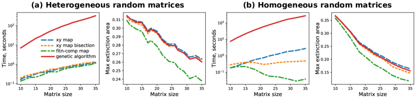
Supplementary Figure S3: Comparison of a genetic algorithm, the $x$-$y$ map (using two procedures for finding the optimum), and the fitness-complexity map for the performance in computing the extinction area of a bipartite system. Two ensembles of random matrices have been considered whose precise definition is in the main text: uniform matrices with $p=1/3$, panel (a), and heterogeneous matrices panel (b). The left plot of each panel shows the computational time (in seconds) as a function of the matrix size $s$, while on the right there is the best extinction area found by each algorithm. The two quantities are the average over an ensemble of $200$ random matrices for each size. The definition of the algorithms and procedure of the matrix generation are explained in the main text. The parameters of the genetic algorithm are: $N=500$, $\mu=0.05$, and $t_{stop}=10^{4}$, while for the bisection of the $x$-$y$ map: $\gamma_{0}=0.8$, $\Delta_{0}=0.2$, $\hat{\Delta}=0.01$.

Figure S3 shows that the $x$-$y$ map with the simplex algorithm finds, on average, a better extinction area than all the other algorithms. The fact that it is even larger than the genetic algorithm should be due to the very large space of the ranking that cannot be reliably explored in reasonable computational times. The bisection method applied to the $x$-$y$ map can be faster than the simplex method (panel (b)), but can be trapped in local maxima and performs a bit poorer, suggesting that the extinction area as a function of the exponent $\gamma$ is not always perfectly concave. The fitness-complexity map performs significantly worse than the other algorithms. It is curious that the computational time decreases with the size in homogeneous matrices. This happens because the transition point, which is close to one for small matrices, increases with the size, and, as a consequence, the computational time to run the map farther from the transition decreases.

S4 Computing the phase transition exponent

From Figure 4 of the main manuscript and Figure S4, it is clear that the phase transition of the fraction of positive scores is not always a sudden jump from $1$ to a number $O(1/n)$. Therefore, to numerically compute the transition exponent one needs a general procedure that gives reliable estimates in all the possible scenarios. We employed the following algorithm:

• Find the largest exponent for which the number of convergent trajectories is $O(1/n)$, $\gamma_{\text{left}}$. To this end, we start simulating the map at a very low exponent, compute the fraction of positive scores, $f_{\text{small}}$, and iteratively increase the exponent using a bisection method to find the point in which a number of positive scores larger than $f_{\text{small}}$ converges.

• Find the smallest exponent for which the number of convergent trajectories is $1$, $\gamma_{\text{right}}$. A similar procedure of the step above is employed.

• Compute the fraction of positive scores, $\{f_{1},\ldots,f_{k}\}$ for a set of evenly spaced exponents between $\gamma_{\text{left}}$ and $\gamma_{\text{right}}$: $\{\gamma_{1},\ldots,\gamma_{k}\}$.

• The critical exponent is the average of the computed gammas weighted by the size of the jumps between them:

  $$\gamma_{c}=\frac{\sum_{i=1}^{k-1}\frac{(\gamma_{i+1}+\gamma_{i})}{2}|f_{i+1}-f_{i}|}{\sum_{i=1}^{k-1}|f_{i+1}-f_{i}|}$$

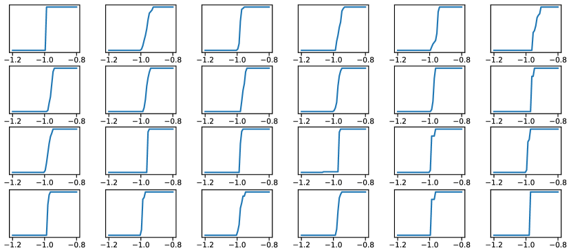
Supplementary Figure S4: Fraction of convergent trajectories as a function of the map exponent in different ecological mutualistic network dataset. Specifically the $24$ largest systems. All the datasets display a phase transition in the number of positive stationary trajectories, and the critical exponent varies.

S5 A stable solution in the condensation phase leads to the bottom-right area of zeros

For a large enough negative value of $\gamma$, the systems lies in the condensed phase and the distribution of scores is characterized by a few scores of order $1$ while all the remaining scores decay to zero exponentially or more than exponentially, see Figure 4 of the main text. This distribution of scores can be parameterized as follows:

$$\mathbf{x}=(\boldsymbol{\epsilon}_{0},\boldsymbol{\epsilon}_{1},\ldots,\boldsymbol{\epsilon}_{k})$$ (S5)

where $\boldsymbol{\epsilon}_{k}$ denotes a set of scores of order $\epsilon_{k}$ and the few scores of order $1$ are in the first block $x_{i}\in\boldsymbol{\epsilon}_{0}$. Let us call $\mathcal{N}_{p}=\{i|x_{i}\in\boldsymbol{\epsilon}_{p}\}$ the set of indexes of the scores that belong to the block $\boldsymbol{\epsilon}_{p}$, and its size $n_{p}=|\mathcal{N}_{p}|$. Moreover let us assume that each block $\boldsymbol{\epsilon}_{p}$ is characterized by an order of magnitude $\epsilon_{p}^{(t)}$ which is much larger than the order of magnitude of the next block, namely, for a sufficiently larger $t$:

$$\frac{x^{(t)}_{i\in\mathcal{N}_{p+1}}}{x^{(t)}_{j\in\mathcal{N}_{p}}}\sim\frac{\epsilon_{p+1}^{(t)}}{\epsilon_{p}^{(t)}}\ll 1$$ (S6)

For the moment, $k$ can be whatever integer larger than $0$, since at least two blocks exist in the condensed phase: the positive scores and the ones going to zero. It will be shown later that, for consistency, the number of scores in each block is of order $1$, implying $k$ to be of the same order of the matrix size.

The only requirement we must impose on eq. S5 if we want to have a consistent solution of the map in the condensed phase is that the pattern of scores is stable under the mapping, i.e. that it reproduces itself after a complete iteration of the mapping. More precisely, a stable solution would require that the scores belonging to the first block are stationary, $x_{i}^{(t+2)}=x_{i}^{(t)}$ $\forall i\in\mathcal{N}_{0}$, while all the others decrease, $x_{i}^{(t+2)}<x_{i}^{(t)}$ $\forall i\notin\mathcal{N}_{0}$, and the property S6 is conserved. What we are going to study now is the $y$ obtained from such an assumption, which conditions are implied by imposing the stability, and which shape the ordered adjacency matrix has in this regime.

The first step is to compute the scores in the opposite layer $\mathbf{y}^{(t+1)}$ given $\mathbf{x}^{(t)}$ having the shape (S5). Let us call the set of nodes in the second layer connected with the smallest $x$-scores (i.e. the block $\boldsymbol{\epsilon}_{k}$) as $\mathcal{M}_{0}=\{j|\exists i\in\mathcal{N}_{k}|A_{ij}=1\}$. We also call the $y$-scores of the nodes in this set as $\boldsymbol{\eta}_{0}=(y_{1},\ldots,y_{m_{0}})$. Thanks to the separation of scales (S6), and the fact that $\gamma<0$, those scores can be approximated as:

$$\tilde{y}_{j\in\mathcal{M}_{0}}^{(t+1)}\simeq\sum_{i\in\mathcal{N}_{k}}A_{ij}\left(x_{i}^{(t)}\right)^{\gamma}\simeq\left(\epsilon_{k}^{(t)}\right)^{\gamma}d_{j}^{k}$$ (S7)

where, for a more compact notation we introduced $d_{j}^{k}=\sum_{i\in\mathcal{N}_{k}}A_{ij}$, which is the number of links from $j$ to a node in the block $k$ of the first layer. One can then iterate the procedure and define $\mathcal{M}_{1}$ as the nodes connected with $\boldsymbol{\epsilon}_{k-1}$ and not with $\boldsymbol{\epsilon}_{k}$, leading to a score of order $(\epsilon_{k-1}^{(t)})^{\gamma}$. In general $\mathcal{M}_{q}=\{j\notin\mathcal{M}_{q-1}|\exists i\in\mathcal{N}_{k-q}|A_{ij}=1\}$, for $q=0,\ldots,k$, defines the nodes whose lowest $x$ neighbour is of order $\epsilon_{k-q}^{(t)}$. Note that, at this point, there is no guarantee that $\mathcal{M}_{q}$, for $q>1$, contains some nodes, however the analysis can be performed without problems allowing for empty sets. It will be found later that the stability of (S5) requires that all the sets $\mathcal{M}_{q}$ contain at least one element. The score of the nodes belonging to $\mathcal{M}_{q}$ (after the normalization step) read:

$$y_{j\in\mathcal{M}_{q}}^{(t+1)}=\frac{\tilde{y}_{j\in\mathcal{M}_{q}}^{(t+1)}}{\langle\tilde{\mathbf{y}}^{(t+1)}\rangle}\simeq\frac{Md^{k-q}_{j}}{\sum_{j\in\mathcal{M}_{0}}d_{j}^{k}}\left(\frac{\epsilon_{k-q}^{(t)}}{\epsilon_{k}^{(t)}}\right)^{\gamma}$$ (S8)

Therefore, one can see that also the ordered $y$-scores form a block structure $\mathbf{y}=(\boldsymbol{\eta}_{0},\boldsymbol{\eta}_{1},\ldots,\boldsymbol{\eta}_{k})$, where scores of order one are only contained in $\boldsymbol{\eta}_{0}$, and the other blocks are of order $\eta_{q}\sim M(\epsilon_{k-q}/\epsilon_{k})^{\gamma}$. Moreover, a counterpart of relation (S6) is satisfied: $\eta_{q+1}/\eta_{q}\ll 1$.

Now one can propagate the $y$-scores to the subsequent step of the $x$-score. Let us define $\mathcal{N}_{0}^{\prime}$ as the set of the first-layer nodes connected with the nodes in $\mathcal{M}_{k}$, the ones with the lowest $y$-score, of order $\eta_{k}^{(t+1)}\sim(\epsilon_{k}^{(t)})^{-\gamma}$. This leads to:

$$\tilde{x}_{i\in\mathcal{N}_{0}^{\prime}}^{(t+2)}\simeq\sum_{j\in\mathcal{M}_{k}}A_{ij}\left(y_{i}^{(t+1)}\right)^{\gamma}\simeq\left(\eta_{k}^{(t+1)}\right)^{\gamma}d_{i}^{k}=\left(\epsilon_{k}^{(t)}\right)^{-\gamma^{2}}d_{i}^{k}$$ (S9)

Since those $x$-scores are much larger than all the other scores, the average $\langle\tilde{\mathbf{x}}^{(t+2)}\rangle$ is dominated by them, and it is of the same order. This implies that the nodes in $\mathcal{N}_{0}^{\prime}$ are of order $1$, and, by imposing the stationary condition of the solution, they must coincide with the order-$1$ scores at time $t$. Therefore $\mathcal{N}_{0}=\mathcal{N}_{0}^{\prime}=\{i|\exists j\in\mathcal{M}_{k}|A_{ij}=1\}$. As a consequence, the ordered adjacency matrix will show a block connecting $\mathcal{N}_{0}$ and $\mathcal{M}_{k}$ at the top-right corner, see Figure S5, and all the other elements below that block are zero (no other nodes of the first layer are connected to nodes in $\mathcal{M}_{k}$). In a similar way one can define $\mathcal{N}_{1}^{\prime}$ as the nodes connected with $\mathcal{M}_{k-1}$ and not with $\mathcal{M}_{k}$. These nodes are of the second leading order, and, to be consistent with a stationary solution of the kind (S5), they must coincide with the nodes in $\mathcal{N}_{1}$. Iterating this procedure one obtains that $\mathcal{N}_{p}=\mathcal{N}_{p}^{\prime}=\{i\notin\mathcal{N}_{p-1}|\exists j\in\mathcal{M}_{k-p}|A_{ij}=1\}$. Note that, to be consistent with the stationary condition, all the $\mathcal{M}_{q}$, $q=1,\ldots,k$ must be non empty, otherwise, if $|\mathcal{M}_{q}|=0$, the nodes in $\mathcal{N}_{k-q}^{\prime}$ are of the same order of the nodes in another block, going against the separation of scales (S6). The consequence of this structure, where no scores in the block $\mathcal{N}_{p}$ are connected to scores in the blocks $\mathcal{M}_{q}$, $q>k-p$, implies the triangular shape of the ordered adjacency matrix shown in Figure S5. The area of zeros below the diagonal of blocks $\mathcal{N}_{p}$-$\mathcal{M}_{k-p}$ is consistent with the behavior observed in Figure 5 of the main text. The shape of the scores belonging to the block $p$ reads:

$$x_{i\in\mathcal{N}_{p}}^{(t+2)}\simeq N\frac{B_{i}^{p}}{\sum_{i^{\prime}\in\mathcal{N}_{0}}B_{i^{\prime}}^{0}}\left(\frac{\epsilon_{p}^{(t)}}{\epsilon_{0}}\right)^{\gamma^{2}}$$ (S10)

where, for simplicity of notation we introduced $B_{i}^{p}=\sum_{j\in\mathcal{M}_{k-p}}A_{ij}\left(d_{j}^{p}\right)^{\gamma}$.

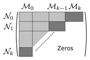
Supplementary Figure S5: Adjacency matrix ordered according to the scores in the condensation regime.

If one assumes that the $B_{i}^{p}$ are approximately of the same order of magnitude for each $p$ and $i$, the scores are: $x_{i\in\mathcal{N}_{p}}\sim N(\epsilon_{p}^{(t)}/\epsilon_{0})^{\gamma\cdot\gamma}/n_{0}$. Under this approximation, the condition that each block $\boldsymbol{\epsilon}_{p}$, with $p>0$, decreases at each step, can be written as follows:

$$\left(\frac{\epsilon_{p}^{(t)}n_{0}}{N}\right)^{\gamma^{2}-1}<1$$ (S11)

Since a decreasing $\epsilon_{p}^{(t)}$ becomes eventually less than $N$, the only possibility is to choose $\gamma<-1$, providing a qualitative upper bound for the condensed phase, equation (4) of the main text.

A further consequence of relation (S10) is that each score in a block must have the same value, $x_{i}=x_{j}=\epsilon^{p}$, $\forall x_{i},x_{j}\in\boldsymbol{\epsilon}^{p}$. Indeed a small difference between two scores in the same block leads to a separation of scales after a sufficiently large number of steps. If, for example, $x_{i}^{(t)}=\delta+x_{i+1}^{(t)}$, with $\delta>0$:

$$\frac{x_{i+1}^{(t+2k)}}{x_{i}^{(t+2k)}}\propto\left(1+\frac{\delta}{x_{i+1}^{(t)}}\right)^{-\gamma^{2k}}\ll 1$$

Implying that two distinct blocks can be created and a new solution (S5) can be written. This consideration has two important consequences. First, this justifies a posteriori the separation of the scales (S6) assumed at the beginning. Second, it implies that all the nodes in the same block must have the same value, and this happens only if they are connected exactly to the same nodes, which happens very rarely in empirical networks. In turns, we expect that the sizes of the blocks are $1$ or a few units. The sub-matrices $\mathcal{N}_{p}$-$\mathcal{M}_{k-p}$ that separate the area of zeros form the rest of the matrix are, therefore, very small, and this can explain the “border of ones” that one typically sees in the ordered matrix in the condensation phase.

S6 Adjacency matrix shape and extinction area

It can be proved that the number of consecutive zeros from the bottom of the matrix (Figure S6a, green area) is proportional to extinction area computed removing rows (S6b). Also the transposed relation is true: the area of contiguous zeros from the matrix right side is proportional to the extinction area calculated by removing columns.

Supplementary Figure S6: The figure shows the equivalence between the area of zeros from the matrix bottom, panel (a) and the extinction area computed removing rows, panel (b). If the first row is removed, the third column gets extinct, and therefore the extinction curve increases by one green block at “fraction of erased rows”$=0.25$. Note that this contribution to the curve is represented by a box with the same shade of green of the extinct column. The removal of the second row leads to the extinction of the first and the fourth columns, therefore the height of the extinction curve is now at three blocks. Iterating the procedure one can see the equivalence between the area of zeros and the extinction area.

Let us start to formalize the area of zeros from the matrix bottom. For each column $j$, the number of consecutive zeros from the bottom is $z_{j}$. It is also useful to define the following row index: $l_{j}=\max_{i}(A_{ij}=1)$, which is the largest $i$ associated to a $1$ in the column $j$. It is easy to see that $z_{j}=N-l_{j}$, where $N$ is the number of rows. For example, in Figure S6a, $l_{1}=2$, $l_{2}=4$, and so on. The area of zeros is:

$$Z=\sum_{j=1}^{M}z_{j}=\sum_{j=1}^{M}(N-l_{j})$$ (S12)

where the sum is over all the $M$ column. We now assume that the rows of the adjacency matrix are ordered according to the ranking at which we want to compute the extinction area. In order to compute this quantity, the first node/row in the ranking is removed. The node in the opposite layer which remains without links corresponds to a column which, without the removed row, is composed of only zeros (for example in the figure S6a, the third column gets extinct). Let us call $e_{1}$ the fraction of extinct columns after one removed row:

$$e_{1}=\frac{1}{M}\sum_{j=1}^{M}\delta_{l_{j},1}$$ (S13)

where the Kronecker delta is equal to $1$ if $l_{j}=1$, meaning that all the other elements of the column are zeros. Iterating this procedure, the fraction of extinct columns at the $k$-th removal step is:

$$e_{k}=e_{k-1}+\frac{1}{M}\sum_{j=1}^{M}\delta_{l_{j},k}=\frac{1}{M}\sum_{j=1}^{M}\theta(k-l_{j})$$ (S14)

which is the fraction at the previous step, plus the new extinct columns. The Heaviside theta function is $1$ only if $l_{j}\leq k$, i.e. the last non-zero element is lesser or equal than the number of removed columns $k$. The sequence of $e_{k}$ from $k=1$ to $N$ defines the extinction curve, implying that the extinction area reads:

$$E=\frac{1}{N}\sum_{k=1}^{N}e_{k}=\frac{1}{NM}\sum_{j=1}^{M}(N-l_{j}+1)=\frac{Z}{NM}+\frac{1}{N}$$ (S15)

where we have used the expression S14 and the fact that $\sum_{i}^{N}\theta(i-l_{j})=N-l_{j}+1$, establishing a connection between the extinction area and the area of contiguous zeros. Note that the term $1/N$ becomes negligible for large matrices, implying the proportionality between $E$ and $Z$. By transposing the matrix, one can obtain the same relation between the extinction area removing the columns and the area of consecutive zeros from the right side of the matrix.

S7 Comparison with the Mariani map

The map generalization proposed in Mariani et al. (2015) reads as follows:

$$\left\{\begin{array}[]{ll}\tilde{f}^{(t)}_{i}=\sum_{j}A_{ij}q^{(t-1)}_{j}&\hskip 14.22636ptf^{(t)}_{i}=\frac{\tilde{f}^{(t)}_{i}}{\langle\tilde{f}^{(t)}\rangle}\\ \tilde{q}^{(t)}_{j}=\left(\sum_{i}\frac{A_{ij}}{\left(f^{(t-1)}_{i}\right)^{\beta}}\right)^{-\frac{1}{\beta}}&\hskip 14.22636ptq^{(t)}_{j}=\frac{\tilde{q}^{(t)}_{j}}{\langle\tilde{q}^{(t)}\rangle}\end{array}\right.$$ (S16)

which is actually different from our symmetric generalization. This can be seen by imposing the substitution $\tilde{f}_{i}=\tilde{x}_{i}$ and $\tilde{q}_{j}=\tilde{y}_{j}^{-1/\beta}$.

$$\left\{\begin{array}[]{ll}\tilde{x}^{(t)}_{i}=\sum_{j}A_{ij}\left(y^{(t-1)}_{j}\right)^{-1/\beta}&\hskip 14.22636ptx^{(t)}_{i}=\frac{\tilde{x}^{(t)}_{i}}{\langle\tilde{x}^{(t)}\rangle}\\ \tilde{y}^{(t)}_{j}=\sum_{i}A_{ij}\left(x^{(t-1)}_{i}\right)^{-\beta}&\hskip 14.22636pty^{(t)}_{j}=\frac{\tilde{y}^{(t)}_{j}}{\langle\tilde{y}^{(t)}\rangle}\end{array}\right.$$

Indeed they find different node rankings, and therefore different extinction areas, as shown in Figure S7 as a function of the map exponent $\gamma$. In particular, it seems that the symmetric generalization finds always a larger or equal extinction area maximum, and the two maximum coincides only if the symmetric map peak is at $\gamma=1$, Figure S7 (b).

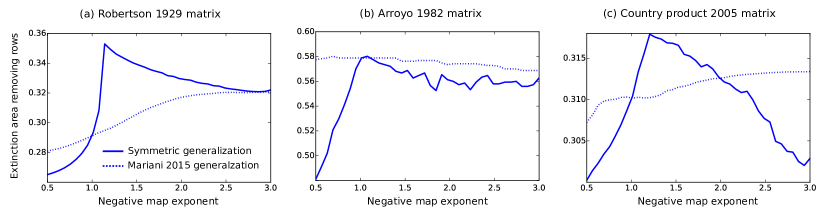
Supplementary Figure S7: Extinction area computed through the Mariani generalization Mariani et al. (2015) and the symmetric one, for three different datasets. Consistently for $\gamma=-1$ both the algorithms are equivalent to the standard one and find the same value of extinction area.

References

- Newman (2018) M. Newman, Networks (Oxford university press, 2018).
- Freeman (1978) L. C. Freeman, Social networks 1, 215 (1978).
- Bonacich (1987) P. Bonacich, American journal of sociology 92, 1170 (1987).
- Katz (1953) L. Katz, Psychometrika 18, 39 (1953).
- Brin and Page (1998) S. Brin and L. Page, Computer networks and ISDN systems 30, 107 (1998).
- Freeman (1977) L. C. Freeman, Sociometry pp. 35–41 (1977).
- Kleinberg (1999) J. M. Kleinberg, Journal of the ACM (JACM) 46, 604 (1999).
- Newman (2005) M. E. Newman, Social networks 27, 39 (2005).
- Estrada and Rodriguez-Velazquez (2005) E. Estrada and J. A. Rodriguez-Velazquez, Physical Review E 71, 056103 (2005).
- Borgatti and Everett (2006) S. P. Borgatti and M. G. Everett, Social networks 28, 466 (2006).
- Mazzolini et al. (2018a) A. Mazzolini, M. Gherardi, M. Caselle, M. C. Lagomarsino, and M. Osella, Physical Review X 8, 021023 (2018a).
- Mazzolini et al. (2018b) A. Mazzolini, J. Grilli, E. De Lazzari, M. Osella, M. C. Lagomarsino, and M. Gherardi, Physical review E 98, 012315 (2018b).
- Mazzolini et al. (2018c) A. Mazzolini, A. Colliva, M. Caselle, and M. Osella, Phys. Rev. E 98, 052139 (2018c), URL https://link.aps.org/doi/10.1103/PhysRevE.98.052139.
- Lazzardi et al. (2023) S. Lazzardi, F. Valle, A. Mazzolini, A. Scialdone, M. Caselle, and M. Osella, Phys. Rev. E 107, 044403 (2023), URL https://link.aps.org/doi/10.1103/PhysRevE.107.044403.
- Gerlach et al. (2018a) M. Gerlach, T. P. Peixoto, and E. G. Altmann, Science advances 4, eaaq1360 (2018a).
- Valle et al. (2020) F. Valle, M. Osella, and M. Caselle, Cancers 12, 3799 (2020).
- Valle et al. (2022) F. Valle, M. Osella, and M. Caselle, Cancers 14, 1150 (2022).
- Watts and Strogatz (1998) D. J. Watts and S. H. Strogatz, Nature 393, 440 (1998).
- Newman (2001) M. E. Newman, Proceedings of the national academy of sciences 98, 404 (2001).
- Cancho and Solé (2001) R. F. I. Cancho and R. V. Solé, Proceedings of the Royal Society of London. Series B: Biological Sciences 268, 2261 (2001).
- Everett (2016) M. G. Everett, Methodological Innovations 9, 2059799116630662 (2016).
- Guillaume and Latapy (2004) J.-L. Guillaume and M. Latapy, Information processing letters 90, 215 (2004).
- Guillaume and Latapy (2006) J.-L. Guillaume and M. Latapy, Physica A: Statistical Mechanics and its Applications 371, 795 (2006).
- Latapy et al. (2008) M. Latapy, C. Magnien, and N. Del Vecchio, Social networks 30, 31 (2008).
- Pavlopoulos et al. (2018) G. A. Pavlopoulos, P. I. Kontou, A. Pavlopoulou, C. Bouyioukos, E. Markou, and P. G. Bagos, Gigascience 7, giy014 (2018).
- Hidalgo and Hausmann (2009) C. A. Hidalgo and R. Hausmann, Proceedings of the national academy of sciences 106, 10570 (2009).
- Daugulis (2012) P. Daugulis, networks 59, 261 (2012).
- Yildirim and Coscia (2014) M. A. Yildirim and M. Coscia, PLOS ONE 9 (2014), ISSN 1932-6203.
- Tacchella et al. (2012) A. Tacchella, M. Cristelli, G. Caldarelli, A. Gabrielli, and L. Pietronero, Scientific reports 2 (2012).
- Cristelli et al. (2013) M. Cristelli, A. Gabrielli, A. Tacchella, G. Caldarelli, and L. Pietronero, PloS one 8, e70726 (2013).
- Tacchella et al. (2018) A. Tacchella, D. Mazzilli, and L. Pietronero, Nature Physics 14, 861 (2018).
- Cristelli et al. (2015) M. Cristelli, A. Tacchella, and L. Pietronero, PloS one 10, e0117174 (2015).
- Domínguez-García and Muñoz (2015) V. Domínguez-García and M. A. Muñoz, Scientific reports 5 (2015).
- Mariani et al. (2015) M. S. Mariani, A. Vidmer, M. Medo, and Y.-C. Zhang, The European Physical Journal B 88, 1 (2015).
- Mariani et al. (2019) M. S. Mariani, Z.-M. Ren, J. Bascompte, and C. J. Tessone, Physics Reports 813, 1 (2019), ISSN 0370-1573, URL https://www.sciencedirect.com/science/article/pii/S037015731930119X.
- Patterson and Atmar (1986) B. D. Patterson and W. Atmar, Biological journal of the Linnean society 28, 65 (1986).
- Ulrich et al. (2009) W. Ulrich, M. Almeida-Neto, and N. J. Gotelli, Oikos 118, 3 (2009).
- Lin et al. (2018) J.-H. Lin, C. J. Tessone, and M. S. Mariani, Entropy 20, 768 (2018).
- Marlin and LaBerge (2001) J. C. Marlin and W. E. LaBerge, Conservation Ecology 5, 9 (2001).
- Hogben (2013) L. Hogben, Handbook of linear algebra (Chapman and Hall/CRC, 2013).
- Cimini et al. (2014) G. Cimini, A. Gabrielli, and F. S. Labini, PLoS One 9, e113470 (2014).
- Allesina and Pascual (2009) S. Allesina and M. Pascual, PLoS computational biology 5, e1000494 (2009).
- Atmar and Patterson (1993) W. Atmar and B. D. Patterson, Oecologia 96, 373 (1993).
- Rodríguez-Gironés and Santamaría (2006) M. A. Rodríguez-Gironés and L. Santamaría, Journal of biogeography 33, 924 (2006).
- Pugliese et al. (2016) E. Pugliese, A. Zaccaria, and L. Pietronero, The European Physical Journal Special Topics 225, 1893 (2016).
- Godrèche (2019) C. Godrèche, Journal of Statistical Mechanics: Theory and Experiment 2019, 063207 (2019).
- Bianconi and Barabasi (2001) G. Bianconi and A. Barabasi, Physical Review Letters 86, 5632 (2001), ISSN 0031-9007.
- Pang and Maslov (2013) T. Y. Pang and S. Maslov, Proceedings of the National Academy of Sciences 110, 6235 (2013).
- Vasques Filho and O’Neale (2020) D. Vasques Filho and D. R. O’Neale, Physical Review E 101, 052305 (2020).
- Koskinen and Edling (2012) J. Koskinen and C. Edling, Social Networks 34, 309 (2012).
- Gerlach et al. (2018b) M. Gerlach, T. P. Peixoto, and E. G. Altmann, Science advances 4, eaaq1360 (2018b).
- Corel et al. (2018) E. Corel, R. Méheust, A. K. Watson, J. O. McInerney, P. Lopez, and E. Bapteste, Molecular Biology and Evolution 35, 899 (2018).
- Servedio et al. (2018) V. D. Servedio, P. Buttà, D. Mazzilli, A. Tacchella, and L. Pietronero, Entropy 20, 783 (2018).
- Morrison et al. (2017) G. Morrison, S. V. Buldyrev, M. Imbruno, O. A. Doria Arrieta, A. Rungi, M. Riccaboni, and F. Pammolli, Scientific Reports 7, 15332 (2017).
- Sciarra et al. (2020) C. Sciarra, G. Chiarotti, L. Ridolfi, and F. Laio, Nature communications 11, 3352 (2020).
- Balland et al. (2022) P.-A. Balland, T. Broekel, D. Diodato, E. Giuliani, R. Hausmann, N. O’Clery, and D. Rigby, Research Policy 51, 104568 (2022).
- Battiston et al. (2017) F. Battiston, V. Nicosia, and V. Latora, The European Physical Journal Special Topics 226, 401 (2017).
- Rahmede et al. (2018) C. Rahmede, J. Iacovacci, A. Arenas, and G. Bianconi, Journal of Complex Networks 6, 733 (2018), ISSN 2051-1310.
- Holme and Saramäki (2012) P. Holme and J. Saramäki, Physics reports 519, 97 (2012).
- Nelder and Mead (1965) J. A. Nelder and R. Mead, The computer journal 7, 308 (1965).