Minimal Interaction Edge Tuning: A New Paradigm for Visual Adaptation

Abstract

The rapid scaling of large vision pretrained models makes fine-tuning tasks more and more difficult on edge devices with low computational resources. We explore a new visual adaptation paradigm called edge tuning, which treats large pretrained models as standalone feature extractors that run on powerful cloud servers. The fine-tuning carries out on edge devices with small networks which require low computational resources. Existing methods that are potentially suitable for our edge tuning paradigm are discussed. But, three major drawbacks hinder their application in edge tuning: low adaptation capability, large adapter network, and high information transfer overhead. To address these issues, we propose Minimal Interaction Edge Tuning, or MIET, which reveals that the sum of intermediate features from pretrained models not only has minimal information transfer but also has high adaptation capability. With a lightweight attention-based adaptor network, MIET achieves information transfer efficiency, parameter efficiency, computational and memory efficiency, and at the same time demonstrates competitive results on various visual adaptation benchmarks.

1 Introduction

Pretraining a large model [10, 9, 3, 22] on general data and fine-tune it on downstream tasks is emerging as the mainstream methodology for computer vision tasks. Knowledge or representation learned from the pretraining makes adaptation to a target domain much easier than training from scratch.

However, some paradoxes begin to emerge within this process or learning paradigm. One natural issue is: if the downstream dataset is small, we cannot afford to and should not store one new fine-tuned model for each downstream visual task. Parameter-efficient fine-tuning (PEFT) methods [14, 32, 15, 28, 19] are proposed to fine-tune large pretrained models with only a small set of trainable parameters, by either inserting small learnable blocks, adding few learnable tokens, or learning low rank decomposition of extra parameters. These methods achieve competitive results on various downstream adaptation tasks with less than 1% trainable parameters compared to full fine-tuning.

While PEFT methods partially solved the storage cost of fine-tuned models, other problems remain. As the scale of pretrained models grows with a blazing fast speed, fine-tuning or even inference itself is becoming unaffordable, especially on devices with limited computational resources. On the other hand, the need for fine-tuning and inference on edge devices (e.g., personal computers, mobile phones or even cameras) rather than on the cloud AI infrastructure is increasing rapidly.

In this paper, we propose a new visual adaptation paradigm: edge tuning, which enables edge devices to fine-tune downstream visual tasks with a small edge network. The edge network merely receives intermediate features/activations from a pretrained model, such that the huge pretrained network is not required to be (either forward or backward) computed on edge devices. Upon the proposed paradigm, we design a new visual adaptation method: Minimal Interaction Edge Tuning, which is based on the side-tuning idea [27, 29]. Methods in this style potentially enables edge-tuning, but the interaction (i.e., features transferred) from the pretrained network to the edge device is too much for an edge device to handle. Our contributions can be summarized as follows:

• We propose a new visual adaptation paradigm: edge tuning, where the pretrained model works as a service in a cloud server, and edge devices fine-tune small edge networks to transfer the pretrained large model towards specific downstream tasks.

• To reduce the interaction between server and edge devices, we reveal that the sum of intermediate features effectively capture essence of the pretrained network, which leads to both minimal interaction and high accuracy.

• We propose a new visual adaptation method: MIET, as an effective means for edge tuning. MIET is parameter-efficient, GPU memory-efficient, computation efficient, and enjoys a low communication overhead between a cloud server and edge devices. Experimental results on various datasets show that MIET is comparable with state-of-the art PEFT methods in visual adaptation accuracy, but enjoys significantly smaller resource consumptions.

2 New Pipeline: Edge Tuning

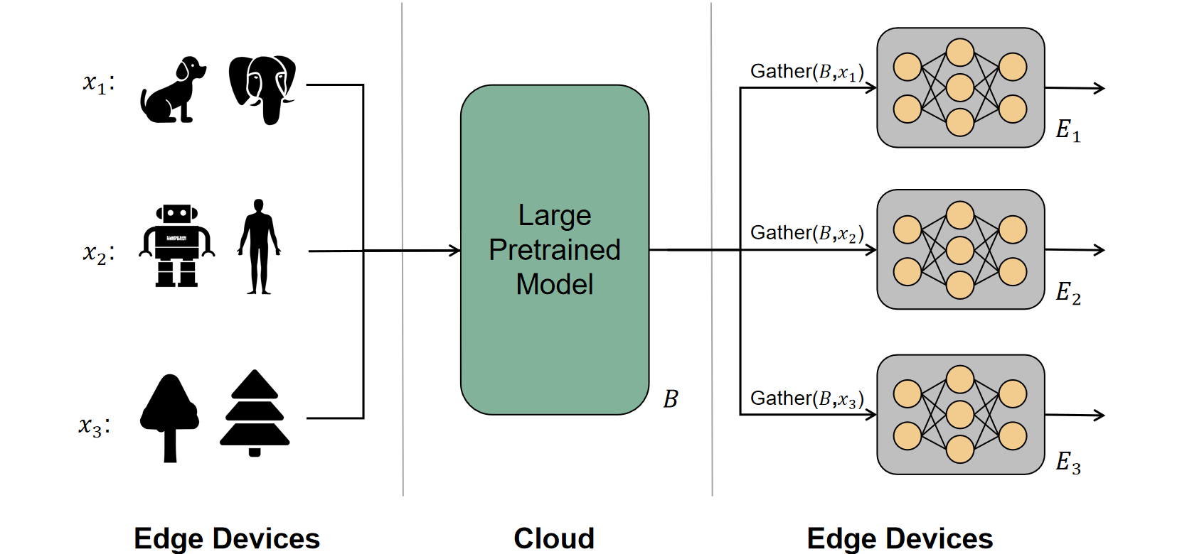
Figure 1: Illustration of Edge Tuning. Visual samples for different tasks ($x_{1},x_{2},x_{3},\dots$) are collected and transferred to the cloud server. Within the cloud server, a large pretrained model $B$ acts as a standalone feature extractor, producing intermediate feature sets $(B,x_{i})$. A gather function compresses this set to $\mathrm{Gather}(B,x_{i})$ to achieve minimal interaction but still keeps essential information in $(B,x_{i})$ for downstream task learning. The gathered features for task $i$ is sent to an edge device $E_{i}$, where the fine-tuning is performed solely on $E_{i}$ with input $\mathrm{Gather}(B,x_{i})$. During inference, the pretrained model extracts features, gather them to a minimal level, transfers only a small chunk of bytes to the edge device, which then makes decisions with small storage, computational, and memory costs.

As illustrated and described in Figure 1, the idea and structure of edge tuning are pretty simple. Computations are split between a pretrained model $B$ (residing in a cloud server) and edge devices. The pretrained model $B$ is general-purpose and pretrained with abundant data and computing resources, which is too big to infer on the edge device. The edge device is mostly likely not powerful enough to store the model $B$ itself, nor does it has the compute or GPU memory resources to forward compute $B$. The solution is to let $B$ extract features and transfer them to the edge device.

Very important but less discussed, the edge device often lacks communication resources. That is, in real world it is often difficult or even impossible to transfer large chunks of data between the edge and the server, e.g., due to bandwidth or energy constraints. Given an input image $x$, $B$ extracts features $(B,x)$ and sends it to the edge device. For example, $(B,x)$ can be the set of activations of all intermediate Transformer blocks’ activations, which contains tens of times more bytes to transfer than that in the input $x$ itself. In such case communication is too heavy a burden for the edge device.

Practical applications, however, are often keen to fine-tune and infer with a model for downstream tasks solely on the edge device with limited storage, compute, memory, and communication capabilities.

2.1 Recipes and Obstacles

Methods that allow to split computations between a large backbone and a small side-network has appeared in the community [27, 29], where the side-network receives features from the backbone but does not send its features back to the computation graph of the backbone. Thus, during fine-tuning, the backbone does not need to compute gradients. This split greatly reduces the compute and (GPU) memory costs of fine-tuning.

An even simpler recipe is linear evaluation, in which final features of the pretrained model $B$ is coupled with a simple fully connected (FC) layer. Fine-tuning is then learning the FC layer, where the transferred features are tiny, the storage, compute and memory costs for edge devices are small, too. Partial-$k$ tuning unfreezes the last $k$ layers of $B$ during fine-tuning. When $k$ is small (e.g., $k=1$), it might be able to fit into edge devices.

However, these methods do not yet fit the purpose of edge tuning we propose in Figure 1. The set of 5 goals in our edge tuning (small storage/parameters, small compute small memory footprint, small communication, high accuracy) cannot be met by existing methods. For example,

• Linear evaluation and partial-$k$ tuning leads to low accuracy in recognition, because they overlook the domain gap between the general-purpose model $B$ and the downstream task.

• Parameter-efficient (PEFT) methods [14, 4] often requires large compute and GPU memory during fine-tuning.

• Side-tuning methods [27] produces and transfers large features $(B,x)$, and the side-network may be too big for the edge device.

2.2 Minimal Interaction Edge Tuning

Our solution, as depicted in Figure 1, meets these requirements by proposing a gather function $\mathrm{Gather}$, which compresses the information in $(B,x)$ to $\mathrm{Gather}(B,x)$. The gathered output is succinct, hence achieving minimal interaction or communication. So long as $\mathrm{Gather}(B,x)$ distills essential information for the downstream task, the small network on the edge device, $E(\mathrm{Gather}(B,x))$ will achieve high accuracy. Because in Figure 1, $E_{i}$ is very small and it does not transfer any features back to $B$, the fine-tuning and inference processes resemble side-tuning methods, which are storage (parameter), compute, and memory efficient, too.

One additional benefit of our pipeline is that the pretrained model is agnostic to downstream tasks. The pretrained model $B$ does not need to store any task-specific parameters or gradients. It simply extract features for any input images. If an input image $x$ is useful in many downstream tasks (edge devices), the pretrained model $B$ only needs to compute its features $(B,x)$ once.

Then, the key and most difficult question is: how to design a gather function that captures essential information in $(B,x)$ and at the same time achieves minimal interaction?

3 Method

We start by studying existing recipes. For example, side-tuning methods can be placed in our pipeline so long as we adopt the following gather function:

$$\mathrm{Gather}(B,x)=\mathrm{Stack}(z_{0},z_{1},\cdots,z_{N}),$$ (1)

where $z_{0}$ is embedding of $x$, and $z_{i}$ is the activations/features of the $i$-th Transformer block in $B$, as illustrated in Figure 2. The ‘Stack’ operator stacks or concatenates all tensors $z_{i}$ together. For example, when the pretrained network $B$ is ViT-B, one $3\times 224\times 224$ input image (0.60MB in size) is required to transfer more than 7.5MB to edge devices!

Figure 2: Architecture of a typical ladder side tuning network [27], where intermediate features $z_{i}$ from the pretrained model $B$ are added to side blocks through side paths. The interaction (features to be transferred) $(B,x)$ are the concatenation of all $z_{i}$ ($i=0,1,\dots,N$).

Because side tuning methods [27, 29] have achieved state-of-the-art accuracy in visual adaptation tasks, it is a natural hypothesis that $\mathrm{Stack}(z_{0},z_{1},\cdots,z_{N})$ contains enough information for downstream tasks. And, we aim to find a gather function $\mathrm{Gather^{*}}$ that can most effectively reduce its size but keep the essential information for downstream tasks.

3.1 Gather Function: Sum is All You Need

Given a typical side tuning structure as shown in Figure 2, learnable side blocks are placed beneath the frozen base network blocks. The $i$-th side block $S_{i}$ takes as input the sum of previous block output $o_{i-1}$ and corresponding feature map $z_{i-1}$ from the pretrained model $B$. Suppose the computing function in side block $S_{i}$ is $F_{i}$, then the output from $S_{i}$ is:

$$o_{i}=F_{i}(o_{i-1}+z_{i-1})+o_{i-1}+z_{i-1}\,.$$ (2)

By induction, we have

$$o_{i}=F_{1}(z_{0})+\Sigma_{l=2}^{i}F_{l}(o_{l-1}+z_{l-1})+\Sigma_{l=0}^{i-1}z_{l}\,.$$ (3)

Then the input for the $i+1$-th side block is $o_{i}+z_{i}$, or equivalently,

$$in_{i+1}=F_{1}(z_{0})+\Sigma_{l=2}^{i}F_{l}(o_{l-1}+z_{l-1})+\Sigma_{l=0}^{i}z_{l}\,.$$ (4)

The first two terms in the right-hand side of Eq. 4 are outputs from learnable side network blocks, while the third term is the sum of intermediate features (or activations) from the pretrained model $B$. It is worth noting that the the first two terms both depend on the side-network, while the third term does not—it is determined by $B$ alone. We name this term (or more generally a term that only depends on $B$) as an external feature term.

To fit into our edge tuning pipeline, $B$ can only send external feature terms to edge devices, a requirement only the third term $\Sigma_{l=0}^{i}z_{l}$ satisfies. This term is developed through repeatedly applying the skip connections.

Furthermore, because side network computations ($F_{i}$) are low rank transformation to achieve parameter efficiency [29], a natural conjecture is that this third term (which is determined by the complex model $B$) contains more complicated features compared to the first two terms (which are determined by the simple computations $F_{i}$). In other words, it is reasonable to guess that the third term, $\Sigma_{l=0}^{i}z_{l}$, contains essential information in $in_{i+1}$. Please note that this conjecture is made with respect to any $i$ ($1\leq i\leq N$), not only the final block (i.e., $i=N$).

Our analysis in the above clearly suggests a simple gather function:

$$\mathrm{Gather^{*}}(B,x)=\mathrm{Sum}(z_{0},z_{1},\cdots,z_{N})\,.$$ (5)

This gather function leads to only $1/(N+1)$ communication overhead compared to the one in Eq. 1. Smaller input to the edge devices also means that the storage, compute, and memory costs will be reduced accordingly. As our experimental results will show in later sections, $\mathrm{Gather^{*}}(B,x)$ does contains essential information for downstream tasks, which leads to high accuracy for them.

$\mathrm{Gather^{*}}(B,x)$ is very simple in its formation, and the idea to sum up intermediate features may seem naive from a first peak. We want to suggest that a simple gather function is the most effective in practice: this gather function incurs almost zero extra computation or memory cost. Furthermore, this simple and natural form is derived from careful analyses of existing methods, which is endorsed by both existing experimental results and supportive conjectures.

3.2 Gather Function: Migrating to Downstream Tasks

One difficulty in handling different downstream tasks are the domain gaps. In some simple tasks with only low-level image patterns, high-level features extracted by a pretrained model may be harmful to the adaptation. In such cases, gathering all the intermediate features altogether is suboptimal.

So we migrate the extracted features to specific downstream tasks by only gathering features from the first $k$ layers, which leads to the final form of our minimal interaction gather function:

$$\mathrm{Gather^{*}}(B,x,k)=\mathrm{Sum}(z_{0},z_{1},\cdots,z_{k})\,,$$ (6)

in which $0\leq k\leq N$. As we emphasized earlier, our hypothesis that the third term in Eq. 4 contains essential information inside $in_{i+1}$ is made for all $i$ ($1\leq i\leq N$). Hence, this final form is also supported by our hypothesis.

We also want to point out that previous side-tuning methods such as [27, 29] correspond to $k=N$ (i.e., use the feature set $\{z_{0},z_{1},\dots,z_{N}\}$ all the way up to the final layer’s output $z_{N}$). However, as our analysis and experiments show, it is both reasonable and beneficial to use $i<N$ for tasks with large domain gaps.

This final form introduces a hyperparameter, $k$, which needs to be set before edge tuning. We select the best $k$ from a candidate set by using the validation set. The candidate set is formed by $N$, $3N/4$ and $N/2$. For example, for ViT-B with 12 layers, we pick $k$ from the set $[6,9,12]$.

Figure 3: Illustration of MIET and other fine-tuning methods. Adapter fine-tunes a model by inserting trainable adapter blocks. LoRA adds trainable low-rank decomposed matrices to parameters. Side-tuning trains a decoupled side network by passing intermediate features to the side network block-wise. MIET adds intermediate features together, and pass the sum to a trainable edge network to adapt to specific task.

3.3 The Proposed MIET Method

With $\mathrm{Gather^{*}}$, our Minimal Interaction Edge Tuning (MIET) method becomes clear and easy to describe. It contains a pretrained base vision transformer network $B$ and a low-rank attention edge network $\mathrm{LAE}$ (which will be introduced latter).

First we gather the intermediate features with $\mathrm{Gather^{*}}$. For base network $B$ with $N$ layers, it receives an input image $x$ and a $k$ for gather function. The forward path of $x$ produces a set of feature maps, Then we gather the feature maps with $\mathrm{Gather^{*}}$ to form a mixed feature map $Z_{\mathrm{mix}}$:

$$Z_{\mathrm{mix}}=\mathrm{Gather^{*}}(B,x,k)\,.$$ (7)

Then the low-rank attention edge network $\mathrm{LAE}$ takes $Z_{\mathrm{mix}}$ as input and output the final tuning result:

$$Z_{\mathrm{out}}=\mathrm{LAE}(Z_{\mathrm{mix}})\,.$$ (8)

From the result in [29], attention block with low-dimensional QKV projection is an effective and efficient structure for visual adaptation. Our experimental results also show that it is very effective for edge tuning. So we adopt this structure for edge network.

As shown in Figure 3, $\mathrm{LAE}$ contains $L$ blocks. Each block contains a layer norm [1] and a low-rank attention, where low-rank attention refers to self-attention with an extremely low QKV hidden dimension $r$ (e.g., hidden dimension equals 16 for feature dimension equals 768). Skip connection is also applied in each block. In practice, we take $L=4$ and $r=32$ for all downstream tasks, and find that such a small edge network scale is already enough for most visual adaptation tasks.

4 Experiments

Table 1: Results on VTAB-1K. “Params”: number of trainable parameters. “MACs Cloud”, “MACs Edge”: multiply–accumulate operations for cloud and edge model during fine-tuning. “GPU Mem Cloud”, “GPU Mem Edge”: GPU memory footprint within cloud and edge devices, respectively during fine-tuning with batch size 32. “Nat.”, “Spe.”, “Str.”: average accuracy for “Natural”, “Specialized”, “Structured” task groups. “Avg.”: group-wise average accuracy. Best results are in boldface.

ViT-B/16	Support	Transfer	Trainable	MACs		GPU Mem		VTAB
	Edge	Overhead	Params	Cloud	Edge	Cloud	Edge
(85.8M)	Tuning	(MB/img)	(M)	$\bm{(\times{10}^{9})}$	$\bm{(\times{10}^{9})}$	(GB)	(GB)	Nat.	Spe.	Str.	Avg.
# of tasks								7	4	8	19
Full fine-tuning		-	85.8	0000	17.57	000	6.09	75.9	83.4	47.6	68.9
BitFit		-	0.10	0000	17.57	000	3.80	73.3	78.2	44.1	65.2
VPT		-	0.56	0000	23.18	000	5.63	78.5	82.4	54.9	72.0
LoRA		-	0.29	0000	21.87	000	3.40	79.5	84.6	59.8	74.5
AdaptFormer		-	0.16	0000	17.60	000	4.11	80.6	84.9	59.0	74.7
FacT		-	0.07	0000	18.67	000	4.81	80.6	85.3	60.7	75.6
SPT-LoRA		-	0.54	0000	20.44	000	5.13	81.9	85.9	61.3	76.4
Linear probing	✓	0.003	000	17.57	0000	0.57	0.07	69.1	77.1	26.8	57.6
Partial-1	✓	0.577	6.75	17.57	01.42	0.57	0.52	69.4	78.5	34.2	60.7
LST	✓	7.503	2.38	17.57	00.51	0.57	2.08	77.6	85.6	59.7	74.3
LAST	✓	4.040	0.66	17.57	00.15	0.57	0.77	80.9	86.2	62.3	76.5
MIET (ours)	✓	0.577	0.38	17.57	00.09	0.57	0.45	81.4	86.4	62.4	76.7

4.1 Experiments on VTAB-1K

We conducted experiments on VTAB with a ViT-B/16 pretrained with ImageNet-21k. Visual Tasks Adaptation Benchmark (VTAB) [34] is a collection of visual adaptation tasks widely used in assessing transferability of pretrained vision models and fine-tuning methods. It is a benchmark composed of 19 tasks, which can be categorized into three groups: Natural, Specialized, and Structured. Each task includes 800 training images and 200 validation images.

Baseline methods.

We compare MIET with various fine-tuning methods. Basically, we divide them into two categories: those potentially support edge tuning and those do not. For the first category, we have linear probing, Partial-1 (which unfreeze the final layer of ViT-B), LST [27], LAST [29] and our method MIET. For the second category, we have BitFit [33], VPT [15], LoRA [14], AdaptFormer [4], FacT [16], SPT-LoRA [8].

Results.

The results on VTAB-1K is shown in Table 1. Methods that support edge tuning are marked with $\checkmark$ in corresponding cell. In the “Transfer Overhead” column, we list the communication cost per image between cloud and edge devices. MIET only requires to transfer 0.58MB of information per image (which roughly equals the size of an original image), lower than other compared methods (except linear probing). This overhead is only about $1/7$ of LAST and $1/13$ of LST. Hence, MIET has met our “minimal interaction” goal.

With respect to trainable parameters, MIET only introduces 0.38M trainable parameters, lower than other methods that support edge tuning. Though MIET requires slightly more trainable parameters than some non-edge tuning methods, this difference is in fact negligible with respect to parameter size of the pretrained model (e.g., MIET:0.38/85.8=0.44% vs. FacT:0.07/85.8=0.08%, both $<1\%$).

We also list the MACs and GPU memory footprint for different methods. For non-edge tuning methods, the whole model are enforced to be fine-tuned on edge devices. For methods that support edge tuning, pretrained model is deployed on a cloud server and edge networks are deployed on edge devices, leading to very low FLOPs and memory footprint on edge devices. MIET requires the lowest MACs and GPU memory (again except linear probing) within edge devices, which are respectively about 1% and 10% of normal PEFT methods.

MIET achieves the highest group-wise accuracy compared to other methods. It has the highest group accuracy for specialized datasets and structured datasets. This result proves that MIET has strong adaptation ability and our $\mathrm{Gather^{*}}$ indeed capture essential information in intermediate features.

4.2 Experiments on Fine-Grained Few-Shot Learning

To further assess the few-shot adaptation ability of MIET, following [16] we run MIET on fine-grained few-shot (FGFS) benchmark, which contains 5 fine-grained datasets: Aircraft [20], Food101 [2], Pets [23], Flowers102 [21] and Cars [17]. We fine-tune the edge network with train set containing 1, 2, 4, 8, 16-shot per class. Experiments are repeated three times with three different random seeds, and we report the average test set accuracy.

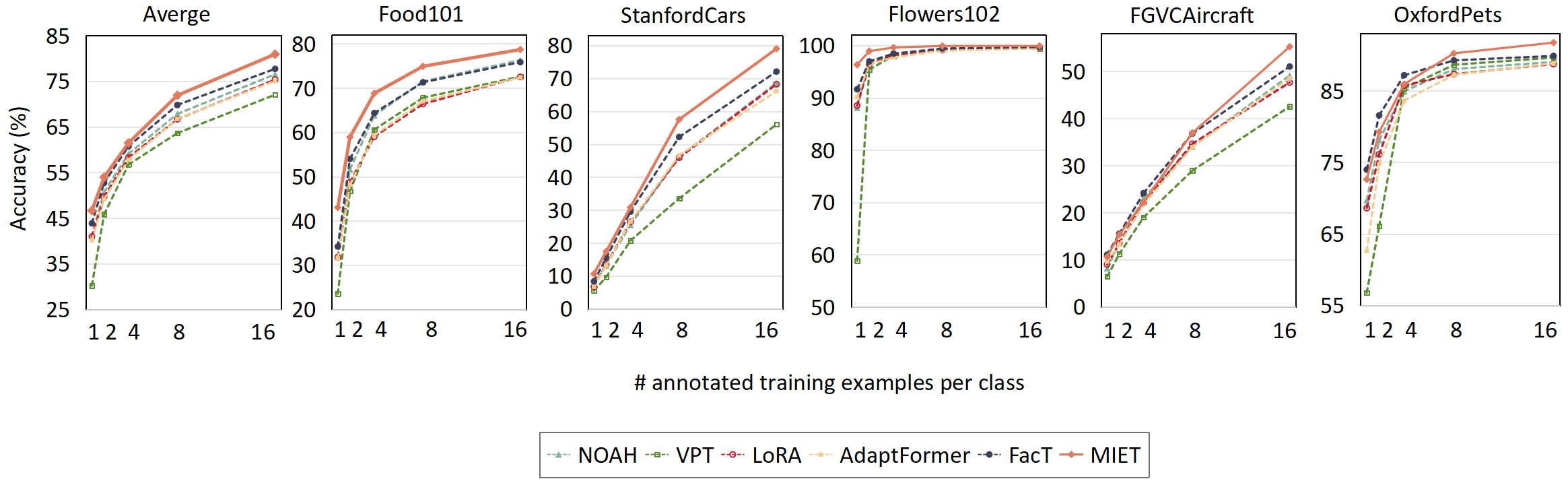
Figure 4: Top-1 accuracy on fine-grained few-shot datasets with train set containing 1, 2, 4, 8, 16-shot per class.

Results.

As shown in Figure 4, the average few-shot accuracy of MIET consistently outperforms other 5 baseline methods in all cases. The average improvement of MIET compared to previous state-of-the-art FacT gets to 3.2% in 16-shot, which is the greatest improvement among all settings.

4.3 Experiments on Domain Generalization

Following the setting in [35], we test the robustness of MIET to domain shifts [36] when they are inevitable. We randomly sample 16 images from each class in ImageNet-1K to form train set. Apart from the validation set from ImageNet-1K [26], we also test the fine-tuned model on four out-of-domain datasets: 1) ImageNet-V2 [25] is collected from different sources than ImageNet but following the same collection protocol, 2) ImageNet-Sketch [31] is composed of sketch images of the same 1,000 classes in ImageNet, 3) ImageNet-A [12] contains adversarially-filtered images, 4) ImageNet-R [11] contains various artistic renditions of ImageNet-1K. We repeat the experiments for three times with different seeds and report average result over three seeds.

Table 2: Results on domain generalization with ViT-B/16 as the pretrained model $B$. Following [35], we randomly sample 16 images from each class in ImageNet-1K, and test the fine-tuned model on test sets with different domain shifts. We report average test accuracy over 3 different random seeds. Best Results are shown in boldface.

	Source	Target
	ImageNet	-Sketch	-V2	-A	-R
Adapter	70.5	16.4	59.1	5.5	22.1
VPT	70.5	18.3	58.0	4.6	23.2
LoRA	70.8	20.0	59.3	6.9	23.3
NOAH	71.5	24.8	66.1	11.9	28.5
MIET (ours)	76.5	37.9	66.5	21.4	37.5

Results.

As shown in Table 2, MIET outperforms previous methods consistently in both the source domain and in generalization to other domains. Compared to the previous the state-of-the-art method NOAH, the accuracy gain of MIET is very significant in ImageNet, ImageNet-Sketch,ImagnetNet-A and ImageNet-R, which are 5.0, 13.1, 9.5 and 9.0 percentage points, respectively. These result verifies the robustness of MIET against test set domain shift.

Table 3: Ablations on removing important components of MIET. “Avg.” denotes the group wise average accuracy on VTAB. $\mathrm{Gather}^{*}$ for (add intermediate features together / use output feature alone). LAE for (use low-rank attention edge network / linear probing).

$\mathrm{Gather}^{*}$	LAE	Avg.
		57.6
✓		59.3
	✓	66.7
✓	✓	76.7

Table 4: Ablations on different block functions with ViT-B/16 as the pretrained model. # Layers denotes the number of layers in edge network. Avg. denotes the group wise average accuracy on VTAB.

Block Func	# Layers	Params (M)	Avg.
LAE	4	0.38	76.7
LAE	8	0.76	76.9
MLP	4	0.38	75.8
MLP	8	0.76	76.1
DWConv	4	0.03	69.8
DWConv	8	0.06	70.2

4.4 Ablation studies

Now we conduct ablation studies on different components of MIET.

Ablations on feature gathering and LAE.

we test the effectiveness of minimal interaction feature gathering ($\mathrm{Gather}^{*}$) and low-rank edge network in our method. Results are shown in Table 4.3. When both of them are not adopted, the method degrade to naive linear probing. When only minimal interaction feature gathering is used, then intermediate features are added for linear probing, the result in the second row reveal a 1.7% gain over naive linear probing, but this improvement is limited. When only LAE is used, the accuracy gain over naive linear probing is 9.1%, which indicates that adding an edge network directly after a pretrained model is useful for visual adaptation, but still lags far behind other fine-tuning methods. When both $\mathrm{Gather}^{*}$ and LAE are adopted, the average accuracy increases to 76.7% (on par with or better than other fine-tuning methods). This ablation shows that both components are important for MIET in visual adaptation, and only when two components are used together can we get the best results.

Ablations on different edge network structure.

We substitute the block function of edge network with MLP and Depthwise convolution (DWConv) [5]. Results are shown in Table 4.3. We can see that while low-rank attention (LAE) and MLP have the same number of parameters, LAE outperforms MLP with about 1% average accuracy lead. When the block function is changed to depthwise convolution, the number of parameters decreases, but the average accuracy also drops by a large margin. Overall, low-rank attention leads to the best performance and parameter efficiency tradeoff.

Ablations on domain migration.

To verify the effect of domain migration with different $k$, we test the respective accuracy on all 19 VTAB datasets for $k=6$, $k=9$ and $k=12$. Results are shown in Figure 5. For Natural and Specialized tasks, $k=12$ (adding all intermediate features) usually lead to the best result. But for structured datasets which have more low-level features, $k=9$ outperforms $k=12$ in 6 out of 9 datasets. These results indicate that in datasets with rich low-level features, intermediate outputs from early layers of the pretrained model are more important.

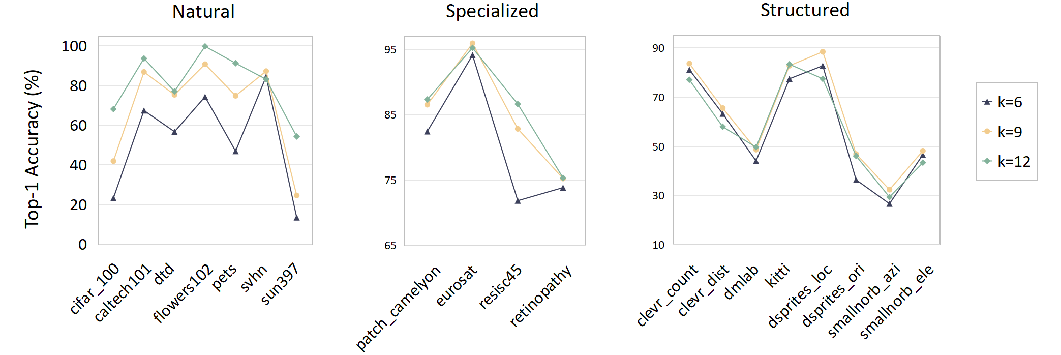
Figure 5: Ablation study on gather function with different $k$ on VTAB. Figures from left to right respectively refer to “Natural”, “Specialized”, and “Structured” task group.

5 Related Work

Parameter-efficient fine-tuning (PEFT) aims at fine-tuning a large pretrained model with only a small amount of trainable parameters. Adapter [13] inserts learnable MLP layers after each attention [30] layer in a Transformer block. AdaptFormer [4] inserts MLP layers to FFN in a parallel form. BitFit [33] fine-tunes the pretrained model to downstream tasks by learning all bias terms within the pretrained model. SSF [18] learns scale factor $\gamma$ and shift factor $\beta$, and $X^{\prime}=\gamma\odot X+\beta$, where $\odot$ is element-wise product. VPT [15] does visual adaptation by learning additional task-specific tokens. VPT-Shallow only inserts learnable tokens before the first later, while VPT-Deep inserts learnable tokens before each later.

LoRA [14] fine-tunes low-rank decomposition matrices of a dense layer instead of fine-tuning dense layers directly. Weights are updated with $W^{\prime}=W+AB$, where $A\in\mathbb{R}^{h\times h^{\prime}}$, $B\in\mathbb{R}^{h^{\prime}\times h}$, $h^{\prime}\ll h$. NOAH [35] combines the structure of Adapter, VPT and LoRA and use evolutionary algorithm to search for best combination.

Another line for visual adaptation is about memory-efficiency. LST [27] proposes to fine-tune a side network which is disentangled from pretrained model, and save memory by freeing pretrained model from back-propagation. DTL [7] considers adding side information back to pretrained network to make a tradeoff between adaptation ability and memory consumption. LAST [29] proposes a low-rank attention side network for effective visual adaptation.

6 Conclusion and Discussion

In this paper, we proposed a visual adaptation paradigm and a method which allows edge devices with extremely low computation resources to finetune large vision model without access to the pretrained model itself. While a pretrained model resides in cloud and provides features that are too large to transfer to the edge device, our minimal interaction edge tuning (MIET) compresses the features while keeping essential information for downstream tasks. The entire fine-tuning process is performed only on the edge device, requesting only limited storage, compute, memory, and communication resources while achieving high accuracy. In particular, we emphasized the communication factor, which has been largely ignored in previous research.

Currently, our MIET is restricted to visual recognition tasks. However, side-tuning has been shown to be able to work for object detection. We will work on this limitation, by extending MIET to object detection and other visual tasks. More vision tasks, such as image and video generation, may also enjoy benefits brought up by MIET. We will also explore other gather functions in the minimal interaction side tuning framework, which may provide even higher accuracy and smaller interaction.

Appendix A Detailed results on VTAB-1K

Here we present a detailed version of Table 1, where per-task accuracy on VTAB-1K datasets are listed.

Table 5: Per-task results on the VTAB-1K benchmark with ViT-B/16 pretrained on IN21k. “Mean Acc” denoted groupwise average accuracy on three VTAB task groups.

	Natural							Specialized				Structured
	CIFAR-100	Caltech101	DTD	Flowers102	Pets	SVHN	Sun397	Patch Camelyon	EuroSAT	Resisc45	Retinopathy	Clevr/count	Clevr/distance	DMLab	KITTI/distance	dSprites/loc	dSprites/ori	SmallNORB/azi	SmallNORB/ele	Mean Acc
Linear probing	64.4	85.0	63.2	97.0	86.3	36.6	51.0	78.5	87.5	68.5	74.0	34.3	30.6	33.2	55.4	12.5	20.0	09.6	19.2	57.6
Full finetuning	68.9	87.7	64.3	97.2	86.9	87.4	38.8	79.7	95.7	84.2	73.9	56.3	58.6	41.7	65.5	57.5	46.7	25.7	29.1	68.9
BitFit	72.8	87.0	59.2	97.5	85.3	59.9	51.4	78.7	91.6	72.9	69.8	61.5	55.6	32.4	55.9	66.6	40.0	15.7	25.1	65.2
VPT	78.8	90.8	65.8	98.0	88.3	78.1	49.6	81.8	96.1	83.4	68.4	68.5	60.0	46.5	72.8	73.6	47.9	32.9	37.8	72.0
LST	59.5	91.5	69.0	99.2	89.9	79.5	54.6	86.9	95.9	85.3	74.1	81.8	61.8	52.2	81.0	71.7	49.5	33.7	45.2	74.3
LoRA	67.1	91.4	69.4	98.8	90.4	85.3	54.0	84.9	95.3	84.4	73.6	82.9	69.2	49.8	78.5	75.7	47.1	31.0	44.0	74.5
AdaptFormer	70.8	91.2	70.5	99.1	90.9	86.6	54.8	83.0	95.8	84.4	76.3	81.9	64.3	49.3	80.3	76.3	45.7	31.7	41.1	74.7
FacT	70.6	90.6	70.8	99.1	90.7	88.6	54.1	84.8	96.2	84.5	75.7	82.6	68.2	49.8	80.7	80.8	47.4	33.2	43.0	75.6
SPT-LoRA	73.5	93.3	72.5	99.3	91.5	87.9	55.5	85.7	96.2	75.9	85.9	84.4	67.6	52.5	82.0	81.0	51.1	30.2	41.3	76.4
LAST	66.7	93.4	76.1	99.6	89.8	86.1	54.3	86.2	96.3	86.8	75.4	81.9	65.9	49.4	82.6	87.9	46.7	32.3	51.5	76.5
MIET	67.8	93.2	76.8	99.7	91.1	87.5	54.0	87.3	95.8	87.1	75.3	84.5	66.8	51.2	83.7	84.0	45.7	33.3	50.3	76.7

Appendix B Imlementation details

We conducted all visual adaptation tasks with a ViT-B/16 pretrained on IN21k as backbone. For VTAB-1K, FGFS and domain generalization tasks, we used Adam optimizer with batch size 32, and cosine learning scheduler to adjust learning rate. Learning rate is selected according to the accuracy on validation set. Following the setting of [15], images were directly resized to 224 × 224 for VTAB-1K. For FGFS and domain generalization tasks, following the setting in [16] and [35], we performed random resize crop and random horizontal flip, and no extra data augmentation tricks were used.

All the experiments were implemented with PyTorch [24].

Appendix C Experiment on varying side input for side tuning

In section 3.1, we conjecture that the third term in Eq. 4 ($\Sigma_{l=0}^{i}z_{l}$, or external feature term), contains essential information in $in_{i+1}$, and thus important to the fine-tune accuracy. So we vary the side input term, by taking $\hat{z_{i}}$ instead of $z_{i}$ as auxiliary input for side block $S_{i+1}$, where:

$$\hat{z_{i}}=\left\{\begin{aligned} &z_{i}&,i<g\\ &z_{i}-z_{i-g}&,i\geq g\end{aligned}\right.$$ (9)

$g$ varies from 1 to N+1. then, $in_{i}=F_{1}(z_{0})+\Sigma_{l=2}^{i}F_{l}(o_{l-1}+z_{l-1})+\Sigma_{l=0}^{i}\hat{z}_{l}$, making:

$$in_{i}=\left\{\begin{aligned} &F_{1}(z_{0})+\Sigma_{k=2}^{i}F_{k}(o_{k-1}+z_{k-1})+\Sigma_{k=0}^{i}z_{k}&,i<g\\ &F_{1}(z_{0})+\Sigma_{k=2}^{i}F_{k}(o_{k-1}+z_{k-1})+\Sigma_{k=i-g+1}^{i}z_{k}&,i\geq g\end{aligned}\right.$$ (10)

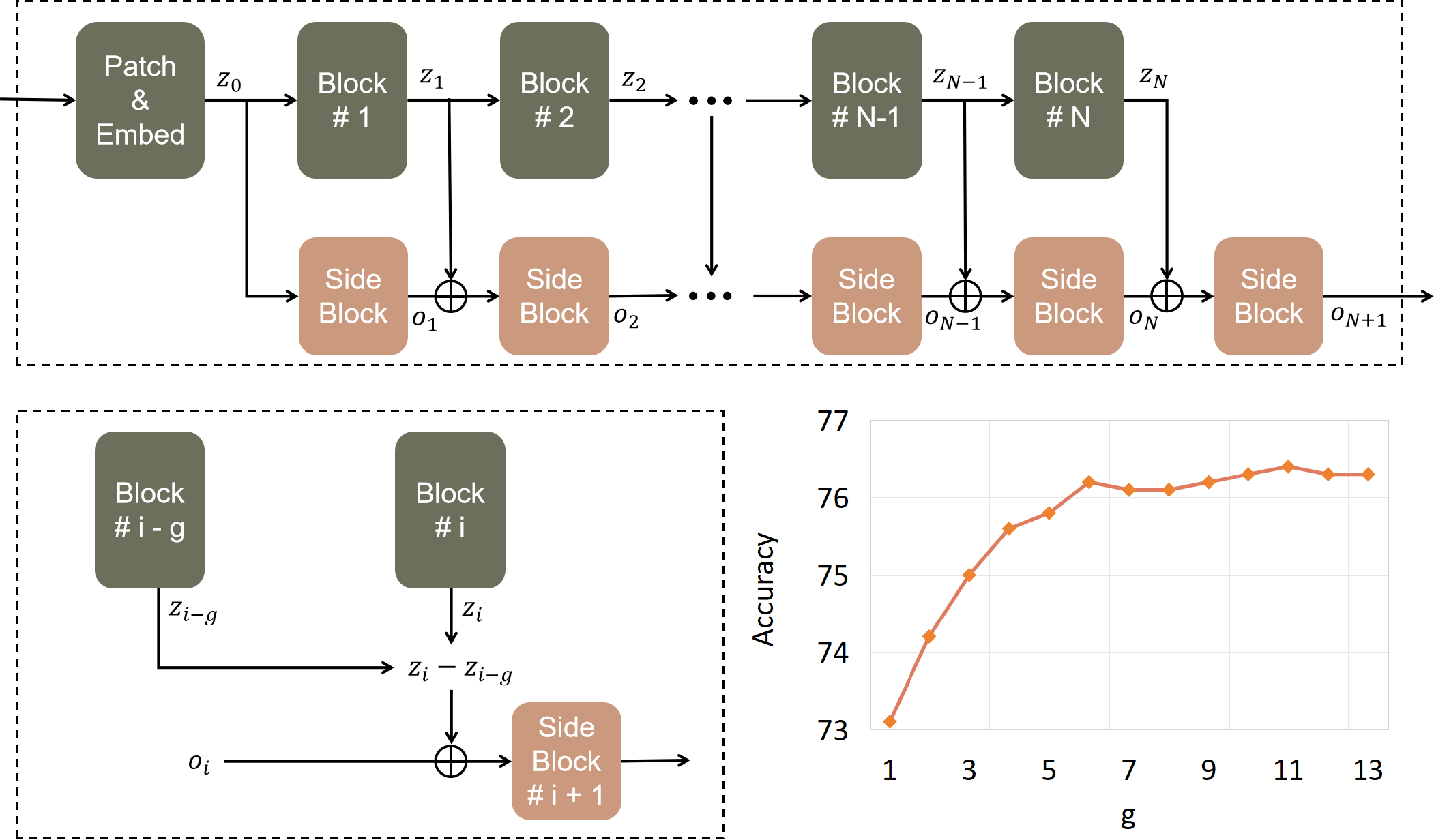
Figure 6: The upper figure shows the architecture of typical ladder side tuning, where intermediate features from pretrained model are added to side blocks through side paths. The lower-left figure shows a modified version of ladder side tuning, where the input from $i$-th side path $z_{i}$ is replaced with $z_{i}-z_{i-g}$. Experiment result on varying intermediate feature input to side network is shown in the lower-right figure. Where $g$ is the hyperparameter which controls the form of intermediate feature input to each side block. Accuracy stands for group-wise average accuracy on VTAB benchnark.

In the experiment, we use ViT-B [6] as backbone, and adopts the low-rank attention structure from [29] as block function in side network. We test the effect of different $g$ on VTAB benchmark, and results are shown in lower-right of Figure 2 (Notice that when $g=13$, the setting falls backs to normal side tuning). From this experiment, we can find that, without previous external feature term from skip connection (the case when $g=1$), overall accuracy suffers from a big cut (73.1). So $z_{i}$ from the side path alone is not enough, the accumulated external feature term is the key for side network. Furthermore, we can discover that increase of $g$ will lead to a higher accuracy, this indicates that more complicated external feature term can result in better model accuracy. The overall accuracy reaches a platform when $g\geq 6$, indicating the benefit of more complicated external feature term is limited.

References

- Ba et al. [2016] Jimmy Lei Ba, Jamie Ryan Kiros, and Geoffrey E Hinton. Layer normalization. arXiv preprint arXiv:1607.06450, 2016.
- Bossard et al. [2014] Lukas Bossard, Matthieu Guillaumin, and Luc Van Gool. Food-101–mining discriminative components with random forests. In European Conference on Computer Vision (ECCV), pages 446–461, 2014.
- Caron et al. [2021] Mathilde Caron, Hugo Touvron, Ishan Misra, Hervé Jégou, Julien Mairal, Piotr Bojanowski, and Armand Joulin. Emerging properties in self-supervised vision transformers. In Proceedings of the IEEE/CVF International Conference on Computer Vision (ICCV), pages 9650–9660, 2021.
- Chen et al. [2022] Shoufa Chen, Chongjian Ge, Zhan Tong, Jiangliu Wang, Yibing Song, Jue Wang, and Ping Luo. Adaptformer: Adapting vision transformers for scalable visual recognition. In Advances in Neural Information Processing Systems (NIPS), pages 16664–16678, 2022.
- Chollet [2017] François Chollet. Xception: Deep learning with depthwise separable convolutions. In IEEE Conference on Computer Vision and Pattern Recognition (CVPR), pages 1800–1807, 2017.
- Dosovitskiy et al. [2021] Alexey Dosovitskiy, Lucas Beyer, Alexander Kolesnikov, Dirk Weissenborn, Xiaohua Zhai, Thomas Unterthiner, Mostafa Dehghani, Matthias Minderer, Georg Heigold, Sylvain Gelly, Jakob Uszkoreit, and Neil Houlsby. An image is worth 16x16 words: Transformers for image recognition at scale. In International Conference on Learning Representations (ICLR), pages 1–21, 2021.
- Fu et al. [2024] Minghao Fu, Ke Zhu, and Jianxin Wu. Dtl: Disentangled transfer learning for visual recognition. In Proceedings of the AAAI Conference on Artificial Intelligence, pages 12082–12090, 2024.
- He et al. [2023] Haoyu He, Jianfei Cai, Jing Zhang, Dacheng Tao, and Bohan Zhuang. Sensitivity-aware visual parameter-efficient fine-tuning. In Proceedings of the IEEE/CVF International Conference on Computer Vision (ICCV), pages 11825–11835, 2023.
- He et al. [2020] Kaiming He, Haoqi Fan, Yuxin Wu, Saining Xie, and Ross Girshick. Momentum contrast for unsupervised visual representation learning. In Proceedings of the IEEE/CVF Conference on Computer Vision and Pattern Recognition (CVPR), pages 9726–9735, 2020.
- He et al. [2022] Kaiming He, Xinlei Chen, Saining Xie, Yanghao Li, Piotr Dollár, and Ross Girshick. Masked autoencoders are scalable vision learners. In Proceedings of the IEEE/CVF Conference on Computer Vision and Pattern Recognition (CVPR), pages 15979–15988, 2022.
- Hendrycks et al. [2021a] Dan Hendrycks, Steven Basart, Norman Mu, Saurav Kadavath, Frank Wang, Evan Dorundo, Rahul Desai, Tyler Zhu, Samyak Parajuli, Mike Guo, et al. The many faces of robustness: A critical analysis of out-of-distribution generalization. In Proceedings of the IEEE/CVF international conference on computer vision (ICCV), pages 8340–8349, 2021a.
- Hendrycks et al. [2021b] Dan Hendrycks, Kevin Zhao, Steven Basart, Jacob Steinhardt, and Dawn Song. Natural adversarial examples. In Proceedings of the IEEE/CVF conference on computer vision and pattern recognition (CVPR), pages 15262–15271, 2021b.
- Houlsby et al. [2019] Neil Houlsby, Andrei Giurgiu, Stanislaw Jastrzebski, Bruna Morrone, Quentin De Laroussilhe, Andrea Gesmundo, Mona Attariyan, and Sylvain Gelly. Parameter-efficient transfer learning for NLP. In International Conference on Machine Learning, pages 2790–2799, 2019.
- Hu et al. [2022] Edward J Hu, Yelong Shen, Phillip Wallis, Zeyuan Allen-Zhu, Yuanzhi Li, Shean Wang, Lu Wang, and Weizhu Chen. LoRA: Low-rank adaptation of large language models. In International Conference on Learning Representation (ICLR), pages 1–13, 2022.
- Jia et al. [2022] Menglin Jia, Luming Tang, Bor-Chun Chen, Claire Cardie, Serge Belongie, Bharath Hariharan, and Ser-Nam Lim. Visual Prompt Tuning. In European Conference on Computer Vision (ECCV), pages 709–727. Springer, 2022.
- Jie and Deng [2023] Shibo Jie and Zhi-Hong Deng. FacT: Factor-tuning for lightweight adaptation on vision transformer. In Proceedings of the AAAI Conference on Artificial Intelligence, pages 1060–1068, 2023.
- Krause et al. [2013] Jonathan Krause, Michael Stark, Jia Deng, and Li Fei-Fei. 3d object representations for fine-grained categorization. In Proceedings of the IEEE Conference on Computer Vision and Pattern Recognition Workshops, pages 554–561, 2013.
- Lian et al. [2022] Dongze Lian, Daquan Zhou, Jiashi Feng, and Xinchao Wang. Scaling & Shifting Your Features: A new baseline for efficient model tuning. In Advances in Neural Information Processing Systems (NIPS), pages 109–123, 2022.
- Liu et al. [2024] Ting Liu, Xuyang Liu, Siteng Huang, Honggang Chen, Quanjun Yin, Long Qin, Donglin Wang, and Yue Hu. DARA: Domain- and relation-aware adapters make parameter-efficient tuning for visual grounding. In Proceedings of the IEEE International Conference on Multimedia and Expo (ICME), pages 1–6, 2024.
- Maji et al. [2013] Subhransu Maji, Esa Rahtu, Juho Kannala, Matthew Blaschko, and Andrea Vedaldi. Fine-grained visual classification of aircraft. arXiv preprint arXiv:1306.5151, 2013.
- Nilsback and Zisserman [2006] M-E Nilsback and Andrew Zisserman. A visual vocabulary for flower classification. In Proceedings of the IEEE Conference on Computer Vision and Pattern Recognition (CVPR), pages 1447–1454. IEEE, 2006.
- Oquab et al. [2024] Maxime Oquab, Timothée Darcet, Théo Moutakanni, Huy Vo, Marc Szafraniec, Vasil Khalidov, Pierre Fernandez, Daniel Haziza, Francisco Massa, Alaaeldin El-Nouby, Mahmoud Assran, Nicolas Ballas, Wojciech Galuba, Russell Howes, Po-Yao Huang, Shang-Wen Li, Ishan Misra, Michael Rabbat, Vasu Sharma, Gabriel Synnaeve, Hu Xu, Hervé Jegou, Julien Mairal, Patrick Labatut, Armand Joulin, and Piotr Bojanowski. Dinov2: Learning robust visual features without supervision, 2024.
- Parkhi et al. [2012] Omkar M Parkhi, Andrea Vedaldi, Andrew Zisserman, and CV Jawahar. Cats and dogs. In Proceedings of the IEEE Conference on Computer Vision and Pattern Recognition (CVPR), pages 3498–3505, 2012.
- Paszke et al. [2019] Adam Paszke, Sam Gross, Francisco Massa, Adam Lerer, James Bradbury, Gregory Chanan, Trevor Killeen, Zeming Lin, Natalia Gimelshein, Luca Antiga, Alban Desmaison, Andreas Kopf, Edward Yang, Zachary DeVito, Martin Raison, Alykhan Tejani, Sasank Chilamkurthy, Benoit Steiner, Lu Fang, Junjie Bai, and Soumith Chintala. PyTorch: An imperative style, high-performance deep learning library. In Advances in Neural Information Processing Systems (NIPS), pages 8026–8037, 2019.
- Recht et al. [2019] Benjamin Recht, Rebecca Roelofs, Ludwig Schmidt, and Vaishaal Shankar. Do imagenet classifiers generalize to imagenet? In International conference on machine learning, pages 5389–5400, 2019.
- Russakovsky et al. [2015] Olga Russakovsky, Jia Deng, Hao Su, Jonathan Krause, Sanjeev Satheesh, Sean Ma, Zhiheng Huang, Andrej Karpathy, Aditya Khosla, Michael Bernstein, Alexander C. Berg, and Li Fei-Fei. ImageNet large scale visual recognition challenge. IJCV, 115(3):211–252, 2015.
- Sung et al. [2022a] Yi-Lin Sung, Jaemin Cho, and Mohit Bansal. LST: Ladder Side-Tuning for parameter and memory efficient transfer learning. In Advances in Neural Information Processing Systems (NIPS), pages 12991–13005, 2022a.
- Sung et al. [2022b] Yi-Lin Sung, Jaemin Cho, and Mohit Bansal. VL-Adapter: Parameter-efficient transfer learning for vision-and-language tasks. In Proceedings of the IEEE/CVF Conference on Computer Vision and Pattern Recognition (CVPR), pages 5227–5237, 2022b.
- Tang et al. [2024] Ningyuan Tang, Minghao Fu, Ke Zhu, and Jianxin Wu. Low-rank attention side-tuning for parameter-efficient fine-tuning, 2024.
- Vaswani et al. [2017] Ashish Vaswani, Noam Shazeer, Niki Parmar, Jakob Uszkoreit, Llion Jones, Aidan N Gomez, Łukasz Kaiser, and Illia Polosukhin. Attention is all you need. In Advances in Neural Information Processing Systems (NIPS), pages 6000–6010, 2017.
- Wang et al. [2019] Haohan Wang, Songwei Ge, Zachary Lipton, and Eric P Xing. Learning robust global representations by penalizing local predictive power. Advances in Neural Information Processing Systems (NIPS), 32, 2019.
- Yin et al. [2023] Dongshuo Yin, Yiran Yang, Zhechao Wang, Hongfeng Yu, Kaiwen Wei, and Xian Sun. 1% vs 100%: Parameter-efficient low rank adapter for dense predictions. In Proceedings of the IEEE/CVF Conference on Computer Vision and Pattern Recognition (CVPR), pages 20116–20126, 2023.
- Zaken et al. [2022] Elad Ben Zaken, Shauli Ravfogel, and Yoav Goldberg. BitFit: Simple parameter-efficient fine-tuning for transformer-based masked language-models. In Proceedings of the 60th Annual Meeting of the Association for Computational Linguistics, pages 1–9, 2022.
- Zhai et al. [2019] Xiaohua Zhai, Joan Puigcerver, Alexander Kolesnikov, Pierre Ruyssen, Carlos Riquelme, Mario Lucic, Josip Djolonga, Andre Susano Pinto, Maxim Neumann, Alexey Dosovitskiy, et al. A large-scale study of representation learning with the visual task adaptation benchmark. arXiv preprint arXiv:1910.04867, 2019.
- Zhang et al. [2022] Yuanhan Zhang, Kaiyang Zhou, and Ziwei Liu. Neural prompt search, 2022.
- Zhou et al. [2023] Kaiyang Zhou, Ziwei Liu, Yu Qiao, Tao Xiang, and Chen Change Loy. Domain generalization: A survey. IEEE Transactions on Pattern Analysis and Machine Intelligence, 45(4):4396–4415, 2023.