A Weighted-Median Model of
Opinion Dynamics on Networks

Abstract

Social interactions influence people’s opinions. In some situations, these interactions result in a consensus opinion; in others, they result in opinion fragmentation and the formation of different opinion groups in the form of “echo chambers”. Consider a social network of individuals, who hold continuous-valued scalar opinions and change their opinions when they interact with each other. In such an opinion model, it is common for an opinion-update rule to depend on the mean opinion of interacting individuals. However, we consider an alternative update rule — which may be more realistic in some situations — that instead depends on a weighted median opinion of interacting individuals. Through numerical simulations of our opinion model, we investigate how the limit opinion distribution depends on network structure. For configuration-model networks, we also derive a mean-field approximation for the asymptotic dynamics of the opinion distribution when there are infinitely many individuals in a network.

1 Introduction

The opinions of people play important roles in society [1, 7], and the influence that people exert on each other through social interactions affect these opinions [21, 5]. However, it is difficult to determine the global opinion landscape that ultimately arises from these interactions. In the study of opinion dynamics, researchers investigate how empirically observed phenomena like polarization (the formation of 2 distinct opinion clusters), fragmentation (the formation of 3 or more distinct opinion clusters), and radicalization can emerge from individual-level social mechanisms (such as cognitive dissonance) [34].

The concept of cognitive dissonance from social psychology gives some insight into opinion dynamics [14]. The theory of cognitive dissonance states that individuals experience psychological stress (so-called “cognitive dissonance”) when they disagree with each other and that individuals change their opinions to relieve this stress [15]. This theory has been used to explain findings about social influence and shifts of political opinions [4, 27]. However, it is infeasible to directly measure the small-scale social forces that people exert on each other. Instead, researchers often study how individual-level mechanisms, which one models using opinion-update rules, produce observed large-scale phenomena (such as polarization).

There are numerous models of opinion shifts [43, 34]. In such models, a typical assumption is that individuals use simple heuristics when navigating complex social domains. When individuals have a social tie in a network, they can influence each other when they interact. Traditionally, one models a network as a time-independent graph, which model pairwise (i.e., dyadic) social ties. However, opinion dynamics have also been studied on more general network structures, such as temporal networks (which allow social ties to change with time) [40, 12] and hypergraphs (which incorporate polyadic social ties) [39, 19].

1.1 Models of continuous-valued opinion dynamics

In the present paper, we suppose that individuals have continuous-valued opinions. (It is also common to study models, such as voter models [37], with discrete-valued opinions.) Such opinions can either take a scalar real value or take a value in a higher-dimensional space. An example situation in which continuous-valued opinions seem appropriate is the choice of the best distribution of state funds to divide between crime prevention and law enforcement, a complex issue in which most people likely hold opinions that lie somewhere between the two extremes of exclusively funding crime prevention or exclusively funding law enforcement.

There is much prior research on opinion models with continuous-valued opinions. Phenomena that have been studied in such models include whether or not they reach a consensus state [38, 25], the time to reach a steady state [32, 44], public versus private opinions [22], and phase transitions between regimes of qualitatively different behaviors [3, 13, 24]. In most opinion models with continuous-valued opinions, the opinion-update rule depends on the mean of the opinions of interacting individuals [34]. Specifically, at each time step, one or more individuals update their opinions based on their own current opinion and a weighted mean of the opinions of the individuals with whom they interact. Well-known examples of such models include DeGroot consensus models [10, 20] and bounded-confidence models [6]

1.2 Median-based models of opinion dynamics

Recently, Mei et al. [29, 30] introduced an opinion model that draws inspiration from cognitive dissonance theory and has an opinion-update rule that is based on the median opinion of interacting individuals. In their model, they supposed that individuals interact with each other in a weighted and directed network. The nodes of the network represent the individuals, who have continuous-valued scalar opinions. In this model, individuals update their opinions asynchronously. At each discrete time, a uniform randomly chosen individual (i.e., node) experiences a cognitive dissonance that is equal to the sum of the absolute differences between their opinion and each of their neighbors’ opinions, with influence weightings that are proportional to edge weights. At each time, this node updates its opinion to a new opinion that minimizes its cognitive dissonance. Using game-theoretic arguments, Mei et al. [30] showed that minimizing the experienced cognitive dissonance entails that individuals shift their opinion to a weighted median of their neighbors’ opinions when they update their opinions. Their model provides a fascinating alternative to opinion models, such as DeGroot models [10, 20] and bounded-confidence models, with update rules that depend on the mean opinions of neighbors [6]. Weighted-median based opinion dynamic models have since been studied with continuous time [18] and for unweighted networks [23].

A possible shortcoming of the weighted-median model of Mei et al. [29] is that individuals do not compromise; they simply assimilate to their surroundings and replace their opinion with the weighted median of their neighbors’ opinions.

In the present paper, we introduce and analyze a synchronous-update analogue of the weighted-median model of Mei et al. [29, 30]. We also modify their model to incorporate self-appraisal, as this allows individuals to not only assimilate the opinions of their neighbors (as in the model of Mei et al.) but also to compromise with them. We investigate the following two questions: (1) How does the final opinion distribution (i.e., the limit opinion distribution) depend on network structure and the initial opinion distribution? (2) Can we effectively describe the dynamics of our model using a mean-field approximation?

Our paper proceeds as follows. In section 2.1, we review a few definitions from network science. In section 2.2, we define our weighted-median model of opinion dynamics. In section 3, we examine the limit opinion distributions of our model for a variety of networks. In section 4, we derive a mean-field approximation of our weighted-median model and then examine its accuracy. Finally, in section 5, we conclude and discuss our findings. In Appendix A, we investigate how the limit opinion distribution depends on the parameters of our opinion-update rule and on network structure. In Appendix B, we derive our mean-field approximation and examine finite-size effects.

2 A weighted-median model of opinion dynamics

We consider a weighted-median opinion model with synchronous opinion updating. We represent each individual as a node of a weighted and directed network. We also suppose that all relationships, which are encoded by the edges of the network, are mutual. Therefore, if there is a directed edge from node $i$ to node $j$, there must also exist an edge from node $j$ to node $i$. However, the weights of these two edges can differ from each other. We normalize the edge weights for each node so that the weights of its outgoing edges (i.e., the out-edges) sum to $1$.

2.1 Some elementary definitions about networks

The simplest type of network is a graph, which is a pair $G=(V,E)$, where $V$ is a set of nodes and $E$ is a set of edges. In a directed graph, each edge has a direction. The directed edge $(i,j)$ emanates from a source node $i$ to a target node $j$. To consider a weighted graph, we assign a positive real value to each edge in $G$. Such an edge weight can encode features such as a social-connection strength or a communication frequency. If nodes $i$ and $j$ are connected by an edge $e$, then the nodes are “adjacent” to each other and are neighbors in the graph $G$. The edge $e$ is “incident” to nodes $i$ and $j$. If $e$ emanates from $i$ to $j$, then $j$ is an “out neighbor” of $i$. The out-degree (respectively, in-degree) of a node is equal to the number of edges that start (respectively, end) at that node.

For a directed network, an “undirected walk” is a sequence of nodes in which each node is adjacent to the next node in the sequence. Two nodes $i$ and $j$ are “weakly connected” if there exist an undirected walk between them. A “largest weakly connected component” of a directed network is a maximal subset of nodes, along with their associated edges, such that all of the nodes are pairwise weakly connected.

Each weighted, directed network $G$ has an associated influence matrix $W\in[0,1]^{|V|}$ [10]. If there is a directed edge from node $i$ to node $j$, the matrix entry $W_{ij}$ gives its weight. If there is no edge from $i$ to $j$, then $W_{ij}=0$. We suppose that $W$ is row stochastic, so the entries of each row sum to $1$. This entails that all nodes have nonzero out-degree, which implies in our opinion model that every node is influenced by at least one other node.

2.2 Synchronous weighted-median opinion updates

Each node $i\in V$ has a time-dependent opinion $x_{i}(t)\in[0,\,1]$ at time $t\in\mathbb{N}_{0}=\{0,1,2,\ldots\}$. The state $x(t)\in[0,1]^{|V|}$ consists of all opinions $x_{i}(t)$ for $i\in V$. Given an initial state $x(0)$, opinions update according to the map

(1) $$x_{i}(t+1)=(1-s)x_{i}(t)+s\,\mathrm{Med}_{i}(x(t)\,;\,W)\,,\quad i\in V\,,$$

where $s\in(0,1)$ is the level of self-appraisal and $\mathrm{Med}_{i}(x(t)\,;\,W)$ denotes the weighted median, which is the unique element of the set

(2) $$\left\{x_{k}\in x(t)\>\>\Big{|}\>W_{i\,k}>0\,,\>\sum_{\{j\,:x_{j}<x_{k}\}}W_{i\,j}\leq\frac{1}{2}\,,\quad\sum_{\{j\,:x_{j}<x_{k}\}}W_{i\,j}\geq\frac{1}{2}\right\}$$

that either minimizes the distance from $x_{k}(t)$ to $x_{i}(t)$ or has the smaller value of the two if there are two elements in the set Eq. 2 with the same distance to $x_{i}(t)$. We refer to this unique element as the weighted-median neighbor opinion and to equation Eq. 1 as our opinion-update rule. See Figure 1 for an illustration of how a single node updates its opinion through the opinion-update rule Eq. 1 for a given influence matrix $W$.

Because $W$ is assumed row-stochastic, all nodes have nonzero out-degrees. Therefore, there are no isolated nodes and the set in Equation 2 is nonempty. Additionally, in our paper, we consider only weakly connected networks. If a network is not weakly connected, one can separately investigate the dynamics of the weighted-median opinion model on each network component. For simplicity, we also follow Mei et al. [29] and assume that all nodes have the same self-appraisal (which they call “inertia”).

(a)

$$W=\begin{bmatrix}0&0.4&0.2&0.3&0.1\\ 0.8&0&0.2&0&0\\ 0&0.8&0&0.2&0\\ 0&0&0&0&1\\ 0.5&0&0&0.5&0\end{bmatrix}$$

(b)

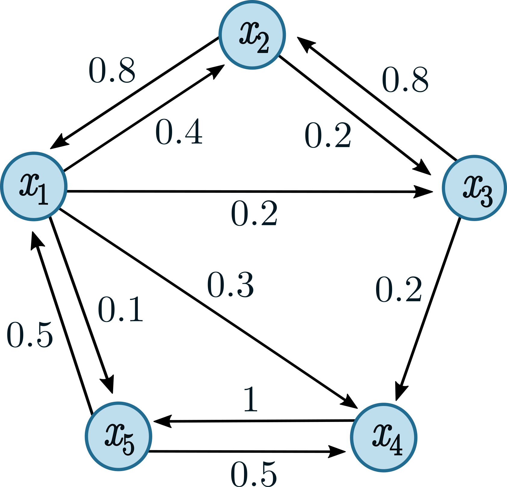
(c)

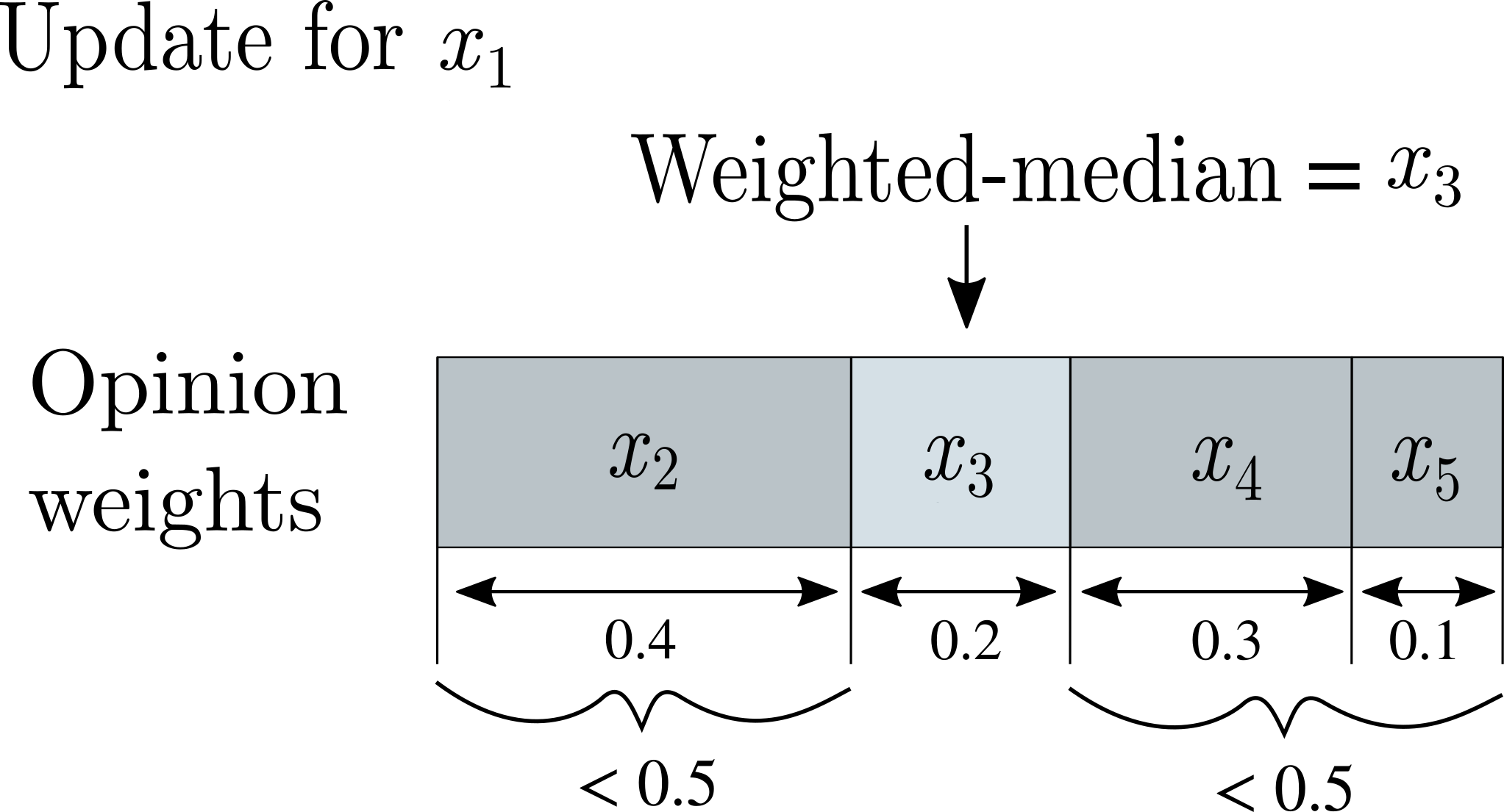
$x_{2}<x_{3}<x_{4}<x_{5}$

Figure 1: An illustration of the weighted-median opinion-update rule (1). (a) An example of an influence matrix and (b) its corresponding directed and weighted network. (c) Node $1$ updates its opinion by adopting the weighted-median neighbor opinion of its neighborhood. Because the update rule (1) is synchronous, all nodes simultaneously update their opinions in this way at each discrete time $t$. [This figure is inspired by Figure 1 of [29].]

3 Limit opinion distributions

Given a network $G$ and an initial opinion state $x(0)$, it is difficult to analytically determine the opinion distribution as time $t\rightarrow\infty$ (i.e., the limit opinion distribution) for the opinion-update rule Eq. 1. Therefore, to examine these distributions, we perform simulations of our weighted-median opinion model on a variety of different networks and for a variety of different initial opinion distributions.

3.1 Simulation specifications

We do not know if a limit opinion distribution exists for all networks $G$ and all initial opinion states $x(0)$. Even when we know that a limit opinion distribution exists, the limit opinion may not occur in finite time.

Therefore, in practice, we examine approximate limit opinion distributions in our numerical simulations. To do this, we introduce a convergence criterion. We interpret the weighted-median opinion model presented in Section 2.2 to have reached a limit opinion distribution at time $t$ if

(3) $$\max_{i\in V}|x_{i}(t)-x_{i}(t+1)|<\varepsilon\,,$$

with $\varepsilon=4.44\times 10^{-16}$ for the examined synthetic networks and $\varepsilon=10^{-6}$ for the examined real-world networks. In all of our numerical experiments, the condition (3) is satisfied in fewer than $10^{6}$ time steps.

For each network and each initial opinion distribution, we sample the initial opinion of each node randomly from the distribution. We then update the node opinions at each discrete time using the update rule Eq. 1 until we satisfy the convergence criterion (3). After convergence, we round all opinions to the $14$th decimal point for simulations on synthetic networks and to the $4$th decimal point for simulations on real-world networks. We then count the number of distinct opinions.

3.2 Network structures

To develop some understanding of the effects of network structure and the initial opinion distribution on the limit opinion distribution, we study the weighted-median opinion model as presented in Section 2.2 on a variety of networks with a variety of initial opinion distributions.

We first consider three deterministic synthetic networks: directed versions of cycle networks, prism networks, and square-lattice networks. In Table 1, we give the definitions and examples of these networks.

Network	Definition	Example
Cycle	For an integer $N\geq 3$, the $N$-node cycle network has the node set $\{v_{j}\,|j\in\{1,\,\ldots\,,\,N\}\}$, directed edges $(v_{j},\,v_{j+1})$ and $(v_{j+1},\,v_{j})$ for $j\in\{1,\,\ldots\,,\,N-1\}$, and directed edges $(v_{N},\,v_{1})$ and $(v_{1},\,v_{N})$.
Prism	For and even integer $N\geq 6$, let $\{v_{j}\,|j\in\{1,\,\dots\,,\,\frac{N}{2}\}\}$ and $\{u_{j}\,|j\in\{1,\,\ldots\,,\,\frac{N}{2}\}\}$ be the node sets of two cycles. The $N$-node prism network is the union of the two cycles with the edges $(v_{j},\,u_{j})$ and $(u_{j},\,v_{j})$ for $j\in\{1,\,\ldots\,,\,\frac{N}{2}\}$.
Square lattice	For integer $k$, the square lattice with side length $k$ is the network with node set $\{(x,y)\,|x,y\in\mathbb{Z}\,\text{ with }\,0\leq x,y\leq k\}$ and edges $((x_{1},y_{1}),(x_{2},y_{2}))$ and $((x_{2},y_{2}),(x_{1},y_{1}))$ for $\|(x_{2}-x_{1},\,y_{2}-y_{1})\|_{2}=1$. (The square-lattice network with side length $k$ has $N=(k+1)^{2}$ nodes.)

Table 1: The deterministic synthetic networks on which we study our weighted-median opinion model presented in Section 2.2

We then consider networks that are generated by directed analogues of two well-known random-graph models [33]: the Barabási–Albert (BA) preferential-attachment model [2] and the Watts–Strogatz (WS) small-world model [42].

To construct an $N$-node BA network, we start with a star network with $m\in\mathbb{N}$ nodes where $m<N$. This initial network has $1$ central node and $m-1$ peripheral nodes, with an undirected edge between the central node and each peripheral node; there are no edges between peripheral nodes. We grow the network by repeatedly adding a single node and connecting it with an undirected edge to $k$ other nodes, with connection probabilities from linear preferential attachment (i.e., according to the BA mechanism). We add nodes until there are $N$ nodes in the network. We then replace all undirected edges by two directed edges, with one in each direction. We generate a single BA network with $m=10$, $k=7$, and $N=2500$. We investigate the limit opinion distribution for this network for different initial opinion distributions.

Our WS network has $N\in\mathbb{N}$ nodes, which we place in a cycle. We start with undirected edges between each node and its $b\in\mathbb{N}$ nearest neighbors. We then rewire edges in the following manner. For each edge $(i,j)$, we uniformly randomly select one of its incident nodes. Suppose without loss of generality that we select node $i$. With probability $p$, we replace the edge $(i,j)$ with an undirected edge $(i,k)$ to a uniformly random node $k\in V\backslash\{i\}$. We treat any resulting multi-edges as single edges. We then replace all undirected edges by two directed edges, with one in each direction.

We generate a single WS network with $b=7$ and $p=0.1$ and investigate the limit opinion distribution for this network for different initial opinion distributions.

We also consider real-world networks of Facebook “friendships” [41] and Twitter (now called “$\mathbb{X}$”) “followerships” [17]. The Facebook networks are undirected, so we replace each edge in them with two directed edges, with one in each direction.

The synthetic networks that we consider each have $N=2500$ nodes and each consists of one big weakly-connected component. The opinion-update rule Eq. 1 requires each edge to have a weight. Because we have no prior information about weights for any of the networks, we assume that each source node $i$ is equally influenced by each of its out-neighbors and set the weight of each directed edge to be $1$ divided by the out-degree of its source node.

3.3 Initial opinion distributions in our simulations

To investigate how the limit opinion distribution depends on the initial opinion distribution, we consider several different initial distributions. Following Mei et al. [29], we build these initial opinion distributions using a beta distribution. Let $\mathrm{Beta}(\alpha,\beta)$ denote the probability distribution with the density function

(4) $$\mathrm{Beta}(\alpha,\beta)=\frac{\Gamma(\alpha+\beta)}{\Gamma(\alpha)\Gamma(\beta)}x^{\alpha-1}(1-x)^{\beta-1}\,,$$

where $\alpha>0$, $\beta>0$, and $\Gamma$ is the Gamma function [35]. We consider the following five initial opinion distributions:

1. Uniform distribution: we independently sample the initial opinion of each node uniformly at random from the interval $[0,1]$.

2. Unimodal distribution: we independently sample the initial opinion of each node from the Beta distribution $\mathrm{Beta}(2,2)$.

3. Skewed unimodal distribution: we independently sample the initial opinion of each node from the $\mathrm{Beta}(2,7)$ distribution.

4. Bimodal distribution: for each node, we sample $X$ from the $\mathrm{Beta}(2,10)$ distribution; we then take the initial opinion of that node to be $X$ with probability $1/2$ and $1-X$ with probability $1/2$.

5. Trimodal distribution: for each node, we sample $X$ from the $\mathrm{Beta}(2,17)$ distribution and sample $Y$ from the $\mathrm{Beta}(12,12)$ distribution; we then take the initial opinion of that node to be $X$, $1-X$, and $Y$ with probabilities $0.33$, $0.33$, and $0.34$, respectively.

3.4 Effect of self-appraisal on the limit opinion distribution

In our numerical simulations, we do not observe any clear dependency of the limit opinion distribution on the self-appraisal $s$. Therefore, we report simulation results only for $s=0.7$ in the main text. In Appendix A.1, we compare the limit opinion distributions for several values of self-appraisal on a variety of networks.

3.5 Limit opinion distributions of our simulations

We now present the results of our simulation study of the limit opinion distribution of our weighted-median opinion model described in Section 2.2 for the synthetic networks, Facebook friendship networks, and Twitter followership networks.

We investigate two features of the limit opinion distributions: (1) the distribution of opinions and (2) how nodes are organized into opinion clusters, which are connected subnetworks in which all nodes have the same opinion.

For each combination of network and initial opinion distribution, we perform a single simulation until our convergence criterion is satisfied. We track the number of opinion clusters and the mean, variance, and kurtosis of the opinion-cluster sizes.

3.5.1 Synthetic networks

In Figure 2, we show histograms of the limit opinion distribution for the cycle network and a self-appraisal of $s=0.7$. We summarize our findings on the size distribution of opinion groups in the main text and show the tabulated summary statistics in Appendix A.2.

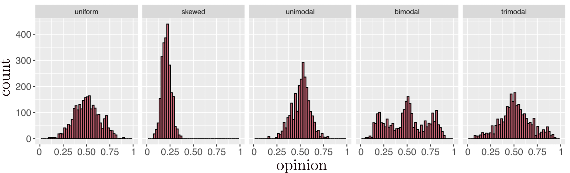
Figure 2: Approximate limit opinion distributions for our weighted-median opinion model presented in Section 2.2 with self-appraisal $s=0.7$ given various initial opinion distributions for a cycle network with $2500$ nodes. Each histogram corresponds to a single approximate limit opinion distribution starting from the indicated initial opinion distribution. We find that the limit opinion distributions are similar for other values of self-appraisal.

We first examine the limit opinion distributions of our weighted-median opinion model presented in Section 2.2 with the uniform, unimodal, skewed, bimodal, and trimodal initial opinion distributions (see section 3.3) for several synthetic networks. For each combination of network and initial opinion distribution, we perform a single simulation until our convergence criterion is satisfied. We then examine properties of the resulting limit opinion distribution.

For the cycle, the prism, and the square-lattice network, we obtain similar mean opinion-cluster sizes for the different initial opinion distributions. They are much smaller than the network size, ranging from $2.48$ to $3.21$ across our simulations for the three networks. However, the kurtoses of the opinion-cluster sizes for the square-lattive network, which range from $26.59$ to $55.15$ in our simulations, are notably larger than for the cycle and prism networks, for which the observed kurtoses range from $0.9$ to $3.29$ in our simulations.

For our WS network, we observe that the number of opinion clusters, as well as the means and variances of the opinion-cluster size distributions are similar for all initial opinion distributions.

The opinion-cluster size kurtoses, which range from $5.70\times 10^{3}$ to $1.52\times 10^{4}$, for our WS network are much larger than the kurtoses for the prism, grid, and cycle network. The large kurtoses imply that the sets of opinion-cluster sizes have many and/or extreme outliers. The opinions of these outliers must be larger than the mean opinion because the mean opinion-cluster size, which ranges from $6.02$ to $6.67$, is much smaller than the network size. Therefore, the large kurtoses indicates that the limit opinion distributions for our WS network have larger opinion clusters than those in the prism, cycle, and square-lattice networks.

For our BA network, the opinion-cluster size kurtoses, which range from $2.17\times 10^{11}$ to $3.54\times 10^{11}$, are even larger than those for our WS network. Additionally, the variances of the opinion-cluster sizes are much larger for our BA network than for our WS network. For our WS network, the largest observed variance of the opinion-cluster size is $27.12$, but our BA network the variance ranges from $6.62\times 10^{4}$ to $8.9\times 10^{4}$. The large kurtoses indicates that the limit opinion distribution for our BA network has opinion clusters that are much larger than the mean opinion cluster, and the large variance indicates that these large opinion clusters occur more frequently.

In our simulations, the opinions in the limit opinion distribution include opinion values throughout the opinion space for the prism, square-lattice, cycle, and WS networks. However, for our BA network, for each initial opinion distribution, a small interval of the opinion space contains all of the opinions in the limit opinion distribution. The length of this interval is about $0.015$, so the limit opinion has support on less than $2$% of the opinion space. Therefore, our simulations suggest that the limit opinion distribution of the weighted-median opinion model presented in Section 2.2 may be fundamentally different for our BA network than for the other synthetic networks.

3.5.2 Facebook friendship networks

We now examine the limit opinion distributions of our weighted-median model presented in Section 2.2 with the uniform, skewed, unimodal, bimodal, and trimodal initial opinion distributions (see section 3.3) for three Facebook friendship networks [41]. In these networks, each node is an individual in one United States university and each edge is a Facebook “friendship” between them. Because we define our weighted-median opinion model on directed networks, we replace each undirected edge with two directed edges, with one in each direction. We set the weight of each directed edge to be 1 divided by the out-degree of the source node. We use networks from Caltech (which has $762$ nodes), Bowdoin (which has $2250$ nodes), and Georgetown (which has $9388$ nodes). For each combination of network and initial opinion distribution, we perform one simulation until our convergence criterion is satisfied. We then examine the resulting limit opinion distribution.

In our simulations of our weighted-median opinion model presented in Section 2.2 on the three Facebook friendship networks, we observe similar distributions of opinion-cluster sizes. The mean opinion-cluster sizes for each of these networks range from $2.55$ to $13.14$, which are much smaller than the network sizes. The kurtoses of the opinion-cluster sizes are notably large. For instance, the kurtosis for the Georgetown network ranges from $3.83\times 10^{8}$ to $2.20\times 10^{9}$. These large kurtoses suggest both that heavy-tailed distributions with large opinion clusters and that they are extreme when they occur. The variances of the opinion-cluster sizes for the Facebook friendship networks are smaller than what we observed for our BA network. Therefore, the Facebook networks have a smaller spread than our BA network in the opinion-cluster sizes around the mean.

For each of the Facebook friendship networks and for all initial opinion distributions, a small number of large opinion clusters include most of the nodes. Additionally, the opinion value of each large cluster is numerically similar to the opinion value of each other large cluster (recall that an opinion cluster is a connected subgraph where all nodes in the subgraph have the same opinion value). However, approximately $10$% of the nodes are instead in small opinion clusters. The opinion value of each of these small clusters varies greatly across clusters. We do not observe this combination of a few large opinion clusters with similar opinion values and many small opinion clusters with dissimilar opinion values in the limit opinion distributions for any of the synthetic networks.

3.5.3 Twitter followership networks

We examine the limit opinion distributions of our weighted-median opinion model presented in Section 2.2) for two Twitter followership networks [17]. In these two networks, each node is a Twitter account that tweeted about a given topic and a directed edge represents a follower relationship between two accounts. The source of an edge is the account that follows, and the target of an edge is the account that is being followed. These two networks involve discussions of the topics Obamacare and abortion. The Obamacare network has $8006$ nodes, and the abortion network has $6114$ nodes. We assign the weight of an edge to be 1 divided by the out-degree of its source node. For each combination of Twitter followership network and initial opinion distribution, we perform one simulation until our convergence criterion is satisfied. We then examine the resulting limit opinion distribution.

We obtain very different limit opinion distributions for the Twitter followership networks than for our synthetic networks. In our simulations with both Twitter followership networks, we observe similar opinion-cluster size distributions for all initial opinion distributions. The mean opinion-cluster sizes are much smaller than the network sizes, and the kurtoses are large. Therefore, the limit opinion distribution has a heavy-tailed opinion-cluster size distribution. Most of the nodes are in one of a few very large opinion clusters with similar opinion values across clusters, but a small proportion of nodes are in small opinion clusters whose opinion values vary greatly across clusters. We also observed this combinations of a few large opinion clusters of similar opinions and a number of smaller opinion clusters with dissimilar opinions in the limit opinion distribution for the Facebook friendship networks.

4 Mean-field approximation

We now derive and study a mean-field approximation for our weighted-median opinion model presented in Section 2.2. We suppose that a set of time-dependent probability distributions govern the probability densities of the opinion at each time step, and we derive difference equations for the time evolution of these densities. Our derivation is inspired by the mean-field approximation of the Deffuant–Weisbuch model in [13].

We are deriving a degree-based mean-field approximation [36], so we assume that the opinions of all degree-$k$ nodes are statistically identical. Therefore, the opinions of all degree-$k$ nodes follow a degree-specific opinion distribution $P_{k}(x,t)$. We assume that these opinions evolve on a network that is generated by a configuration model with a prescribed degree distribution [16]. We also assume that the network is “annealed”; therefore, at each time step, we rewire the edges of the configuration-model network while preserving the in-degree and out-degree of each node [11]. In this section, we give an intuitive explanation for the equations in the mean-field approximation. In Appendix B.1, we give the details of our derivation of this approximation.

Consider the degree distribution $\{q_{l}\}$. For each $l\in\mathbb{N}$, let $q_{l}$ be the probability that a uniform randomly selected node has degree $l$. Let $v\in V$ be a uniformly random degree-$k$ node at time $t\in\mathbb{N}_{0}=\{0,\,1,\,\ldots\,\}$. By assumption, the node’s opinion follows the distribution $P_{k}(x,t)$. To update node $v$’s opinion, we calculate out weighted-median neighbor opinion of its $k$ neighbors. Because the network is annealed, the opinion distribution of each of these neighbors is asymptotically equivalent as the network size (i.e., the number of nodes) tends to infinity. Let $\phi(x,t)$ denote the opinion distribution of a neighbor of node $v$ at time $t$. We can then write

$$\phi(x,t)=\sum_{l}\pi_{l}P_{l}(x,t)\,,$$

where $\pi_{l}$ is the asymptotic probability that a uniformly random neighbor of $v$ has degree $l\in\mathbb{N}$ as the network size goes to infinity. The opinion distribution $\phi(x,t)$ is independent of the degree $k$. Let $\Phi(x,t)$ be the cumulative density function of $\phi(x,t)$.

In the asymptotic limit of infinitely many nodes, the opinions of node $v$’s neighbors are $k$ independent samples from the distribution $\phi(x,t)$. To find the distribution of our weighted median of these $k$ opinions, we use the theory of “order statistics” [9] and find that our weighted-median neighbor opinion has the distribution

$$\theta_{k}(x,t)=\begin{cases}\frac{k!}{m!m!}\phi(x,t)\Phi(x,t)^{m}\left(1-\Phi(x,t)\right)^{m}\,,\,\>\text{$k=2m+1$ (i.e., odd $k$)}\\ \frac{k!}{(m-1)!m!}\phi(x,t)\big{(}\Phi(x,t)\left(1-\Phi(x,t)\right)\big{)}^{m-1}c(x,t)\,,\,\>\text{$k=2m$ (i.e., even $k$)}\,,\end{cases}$$

where $c(x,t)$ is a probability distribution that accounts for the fact that there can be two candidates for our weighted-median neighbor opinion when $v$ has an even number of neighbors. See Appendix B.1 for further details about the definition of $c(x,t)$.

To update its opinion, node $v$ adjusts its opinion towards its weighted-median neighbor opinion. The self-appraisal $s$ controls the magnitude of this opinion shift. Because we only know the distributions of opinions (rather than, e.g., the precise opinion of each node), this opinion shift corresponds to updating the opinion distribution $P_{k}(x,t)$ of degree-$k$ nodes using the equation

(5) $$P_{k}(x,t+1)=\frac{1}{s}\int_{y\in[0,1]}\theta_{k}\left(\frac{x+(s-1)y}{s},t\right)P_{k}(y,t)\,\mathrm{d}y\,.$$

The above procedure holds for any “degree class” $k$ (i.e., for all nodes with degree $k$ for each value of $k$). From the opinion distribution of each degree class, we obtain the global opinion distribution

(6) $$P(x,t)=\sum_{k}q_{k}P_{k}(x,t)\,.$$

The system (6) is a mean-field approximation of the opinion-update rule Eq. 1.

4.1 Specifications for testing the accuracy of our mean-field approximation (6)

We do not know how to analytically solve (6). For a given network and a given initial opinion distribution, we want to investigate how well the mean-field approximation (6) describes the evolution the model presented in Section 2.2. Therefore, we solve (6) numerically and compare our solutions to empirically estimated opinion densities from direct numerical simulations.

We solve the mean-field approximation (6) numerically by discretizing the opinion space into $1025$ equally spaced values and performing first-order interpolation to evaluate $\theta_{k}$ between these values. We obtain numerical solutions of the same accuracy when we instead discretize the space into $2050$ values. For each network, we calculate the degree distribution $q_{k}$ using the network’s empirical degree distribution. To ensure numerical stability of our solution, we lump all degree classes of degree $1000$ or above into a single degree class. For further details on this lumping scheme, see Appendix 13.

We investigate the time evolution of the accuracy of the mean-field approximation (6) for all of our networks. The mean-field approximation does not account for the direction of edges, so we disregard edge directions when we solve (6) . We consider three deterministic synthetic networks (complete networks, cycle networks, and prism networks), the BA and WS random-graph models (see Section 3.2 for our choices of parameter values), and networks that we generate using a configuration model [16, 33] with nodes of two degree classes, $k_{1}=11$ and $k_{2}=101$, with associated probabilities $q_{k_{1}}=0.9$ and $q_{k_{2}}=0.1$. These configuration-model networks are examples of $(k_{1},k_{2})$-regular random graphs [31]. For each of the three random-graph models, we construct $100$ networks with $2500$ nodes each. In Appendix B.2, we examine the accuracy of the mean-field approximation (6) for networks of different sizes. We also study three Facebook friendship networks and two Twitter followership networks (see Section 3.2).

4.2 Accuracy of the mean-field approximation (6)

We explore the accuracy of the mean-field approximation (6) by comparing numerical solutions of them with empirically estimated opinion densities from direct numerical simulations of the opinion-dynamics model presented in Section 2.2. As we will discuss shortly, the accuracy of the mean-field approximation depends in a nontrivial way both on the self-appraisal value and on the network structure.

We perform a variety of numerical experiments. For all networks, we sample the initial opinions of the nodes uniformly at random. For the synthetic networks and the Bowdoin Facebook friendship network, we estimate the limit opinion distributions from $100$ independent simulations with different sets of initial node opinions. Each simulation that uses a random-network model employs a different network that we construct using that model. Because of the large network sizes of the Georgetown Facebook network and both Twitter followership networks, we estimate the limit opinion distributions from $25$ independent simulations with different sets of initial node opinions. For the Caltech Facebook network, we use $300$ independent simulations with different sets of initial node opinions.

In Figure 3, we plot the natural logarithm of the root-mean-square error (RMSE) between our mean-field approximation (6) and our weighted-median opinion model presented in Section 2.2 We observe that the RMSE increases with time and that the RMSE increases faster for larger values of self-appraisal.

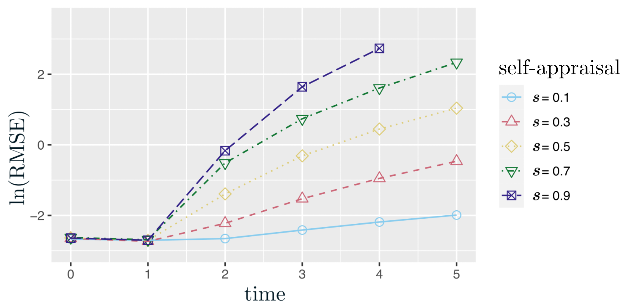
Figure 3: The natural logarithm of the root-mean-square error (RMSE) between our mean-field approximation (6) and our weighted-median opinion model presented in Section 2.2 for a variety of self-appraisal values $s$ as a function of discrete time $t$ for $(k_{1},k_{2})$-regular configuration-model networks with nodes of degrees $k_{1}=11$ and $k_{2}=101$ with associated probabilities $q_{k_{1}}=0.9$ and $q_{k_{2}}=0.1$. At first, the mean-field approximation accurately describes the evolution of the opinion distribution, but the accuracy subsequently deteriorates, with substantial deterioration when $s$ is not small.

To investigate why the RMSE error increases faster for larger values of self-appraisal, we examine a sample mean $\overline{P}(x,t)$ of the opinion densities from our weighted-median opinion model presented in Section 2.2 and the numerical solution $\hat{P}(x,t)$ of our mean-field approximation (6) for self-appraisal values of $s=0.1$ and $s=0.9$ (see Figure 4). For $s=0.9$, the empirical distribution and mean-field approximation eventually diverge from each other. The mean-field approximation evolves towards a Dirac delta function, whereas the empirical opinion distribution retains some spread in the opinion values. For $s=0.1$, the mean-field approximation underestimates the opinion spread at later times, but this occurs much less severely than for $s=0.9$.

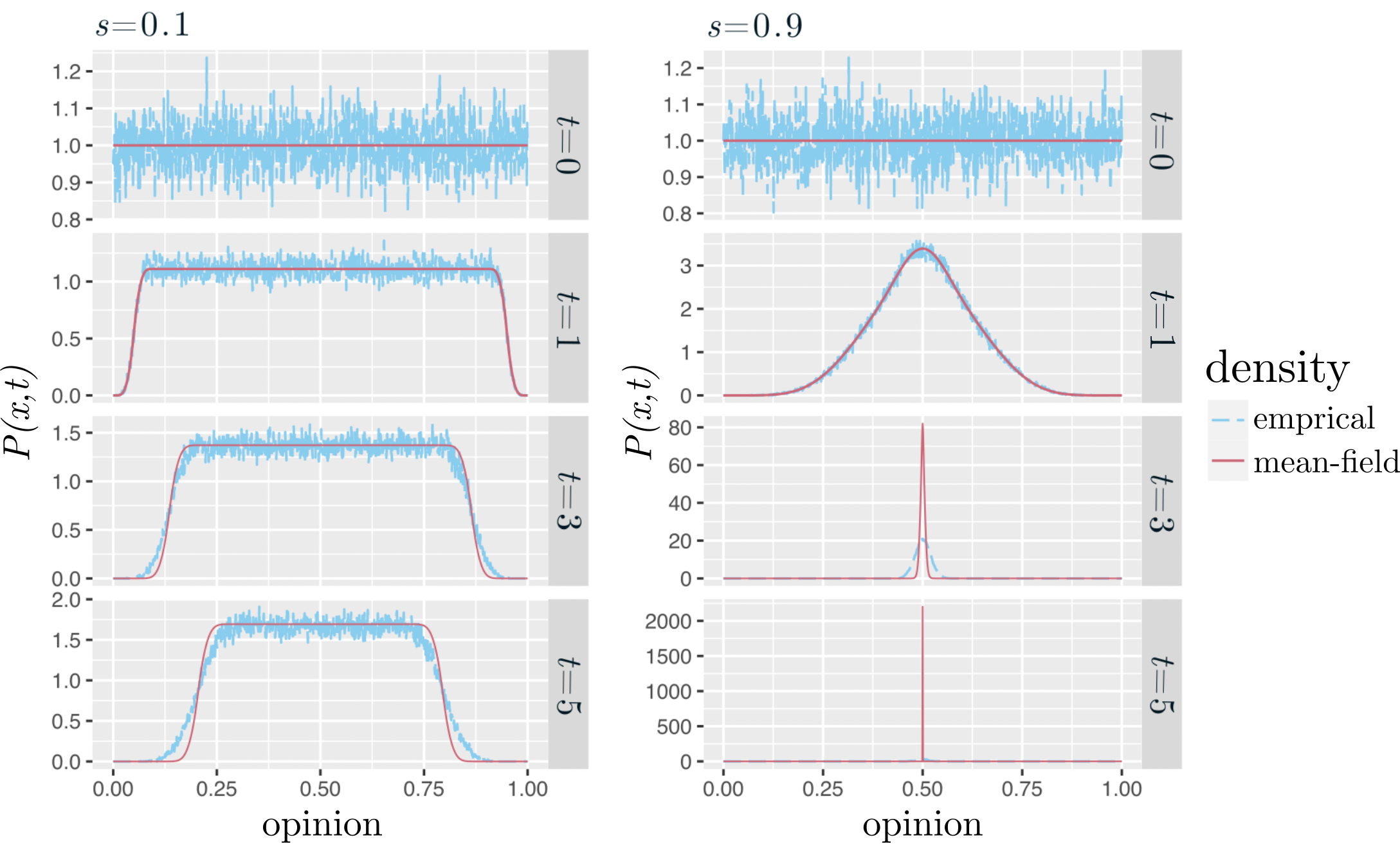
Figure 4: Time evolution of the empirical opinion distribution of our weighted-median opinion model presented in Section 2.2 and the mean-field approximation (6) for self-appraisal values of (left) $s=0.1$ and (right) $s=0.9$ on configuration-model networks from (top) time $t=0$ to (bottom) time $t=5$. The $(k_{1},k_{2})$-regular configuration-model networks have nodes with degrees $k_{1}=11$ and $k_{2}=101$ with associated probabilities $q_{k_{1}}=0.9$ and $q_{k_{2}}=0.1$. For $s=0.1$, the mean-field approximation gives a reasonable but imperfect approximation of direct numerical simulations of our weighted-median opinion model presented in Section 2.2. However, for $s=0.9$, the mean-field approximation eventually evolves towards a Dirac delta function, whereas the empirical opinion distribution from our weighted-median opinion model does not.

In Figure 5, we plot the natural logarithm of the RMSE between our mean-field approximation (6) and our weighted-median opinion model presented in Section 2.2 for a variety of self-appraisal values $s$ for the cycle network. In contrast to the RMSE for the configuration-model networks, the RMSE for the cycle network does not increase faster for larger values of self-appraisal. Instead, of the examined values of $s$, the RMSE is the largest for $s=0.5$ and smallest for $s=0.1$ and $s=0.9$. After time $t=3$, the RMSE increases at a similar rate for all examined values of $s$. The RMSE behavior for the WS networks is similar to that for the cycle network. These are the only two of the examined network types for which the maximum observed RMSE occurs at self-appraisal values other than $s=0.9$.

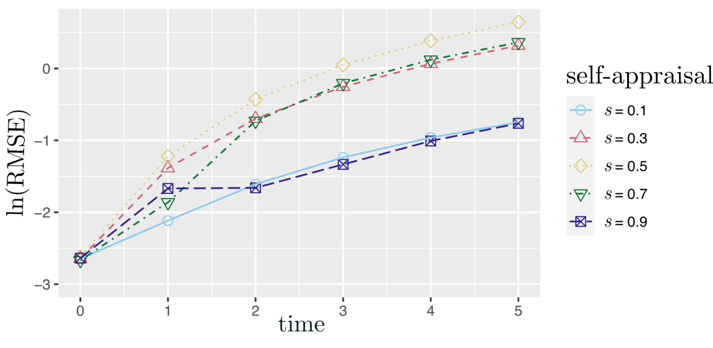
Figure 5: The natural logarithm of the root-mean-square error (RMSE) between the mean-field approximation (6) and our weighted-median opinion model presented in Section 2.2 for cycle networks. The accuracy of the mean-field approximation does not depend monotonically on the self-appraisal $s$.

In Figure 6, we plot the natural logarithm of the RMSE between our mean-field approximation (6) and our weighted-median opinion model for a variety of self-appraisal values $s$ for the Obamacare Twitter followership network. For $s\geq 0.3$, the RMSE stays almost the same after one time step before increasing noticeably, with faster increases for larger values of $s$. For $s=0.1$, the RMSE increases substantially in the first time step and subsequently increases slowly. Based on our simulations, there is a transition in $s$ between these two qualitatively different behaviors. We observe similar patterns for the RMSE for all three Facebook friendship networks and both Twitter followership networks. In Appendix B.3, we investigate the transitional behavior (to examine whether the transition is abrupt or smooth in nature) of the RMSE between $s=0.1$ and $s=0.3$ for the Georgetown Facebook friendship network. Based on these computations, the transition appears to be smooth.

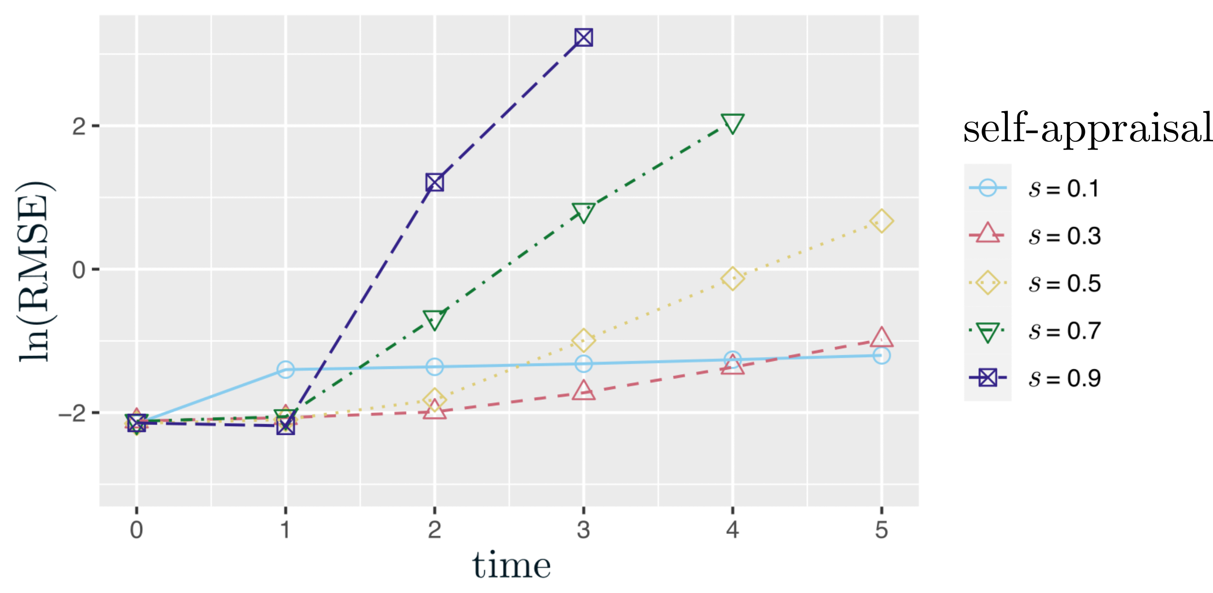
Figure 6: The natural logarithm of the RMSE between our mean-field approximation (6) and our weighted-median opinion model presented in Section 2.2 for the Obamacare Twitter followership network. For small self-appraisal values $s$, the RMSE initially increases notably and subsequently increases less noticeably. By contrast, for larger self-appraisal values, the RMSE is initially almost constant and subsequently increases sharply. We observe a similar pattern for our other real-world social networks.

5 Conclusions and discussion

We formulated and studied a synchronous-update analogue of the asynchronous-update weighted-median opinion model of Mei et al. [29]. We numerically explored our model’s limit opinion distributions and the size distribution of opinion clusters in this limit for a variety of networks. We also derived a mean-field approximation of the evolution of opinion densities, and we examined the accuracy of this approximation.

In our numerical computations, we demonstrated that the opinion-cluster size distributions of the limit opinion distribution depend significantly on network structure. For example, in the examined Facebook “friendship” and Twitter followership networks, we observed that the limit opinion distributions consist of a few large opinion clusters (which together include most nodes of the networks) along with a set of much smaller opinion clusters. We found that the opinions of the large opinion clusters are close to each other in opinion space but that the opinions of the small clusters are spread throughout opinion space. By contrast, for a Barabási–Albert network, we observed that all opinions in the limit opinion distribution are close to each other in opinion space. It is worthwhile to further investigate the different qualitative behaviors of our weighted-median opinion model on different networks.

We also derived and numerically simulated a mean-field approximation of our weighted-median model. We saw in our numerical simulations that the accuracy of our mean-field approximation depends on the amount of self-appraisal. The nature of this dependency depends on the structural characteristics of the network on which the opinions evolve.

There are many ways to build on our work. For example, we do not know if convergence is guaranteed for our synchronous-update weighted median model. There are known criteria for convergence of bounded-confidence models [26] and for the synchronous weighted-median model [30], however, these are not applicable to our model. Therefore, characterizing when convergence is guaranteed may be a fruitful direction for future work. Additionally, we assumed that self-appraisal is constant in time and is homogeneous across all individuals. One can relax both of these assumptions in a way that is reminiscent of the DeGroot–Friedkin model [20]. Our mean-field approximation does not account for asymmetric relationships, and it is desirable to develop approximations that allow one to investigate such situations.

As in other models of opinion dynamics, it is also worth studying bifurcations between qualitatively different regimes (such as opinion consensus, polarization, and fragmentation) in our weighted-median model. It is also important to examine how network structure (such as degree heterogeneity, local clustering, and community structure) affect its opinion dynamics. One can also study how media and other sources of information affect peoples opinions [8] and extend our model to cover multidimensional and interconnected opinions [28].

Our work sheds light on the dynamics of opinion models that build on weighted-median mechanisms of opinion updates [29, 30, 18, 23]. Opinion-dynamics models with opinion updates that are based on medians offer an interesting complement to the much more common mean-based models, and it is worthwhile to explore them further. It is particularly relevant to evaluate which real-world opinion-evolution settings are better described by median-based versus mean-based opinion updates.

Appendix A Limit opinion distribution our weighted median model presented in Section 2.2

A.1 Effect of self-appraisal on the limit opinion distribution

In Figures 7–9, we show the limit opinion distributions of our weighted median opinion-dynamics model presented in (2.2) on a square-lattice network, the WS network, and the Georgetown Facebook friendship network for several self-appraisal values and several different initial opinion distributions (see section 3.3). The synthetic networks each have $2500$ nodes, and the Georgetown network has $9388$ nodes. We observe that the limit opinion distributions are qualitatively similar for the different self-appraisal values.

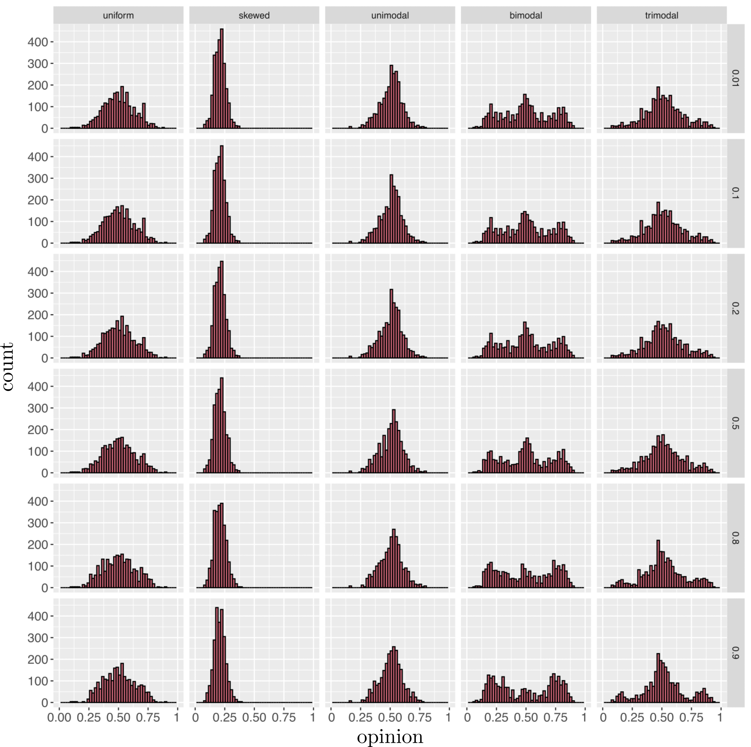
Figure 7: Limit opinion distributions of our weighted median model presented in Section 2.2 for a square-lattice network for several initial opinion distributions and self-appraisal values. Each column has the same initial opinion distribution, and each row has the same self-appraisal value. The limit opinion distributions in each column are qualitatively similar to each other, so it seems that the self-appraisal value has little effect on the limit opinion distribution for the square-lattice network.

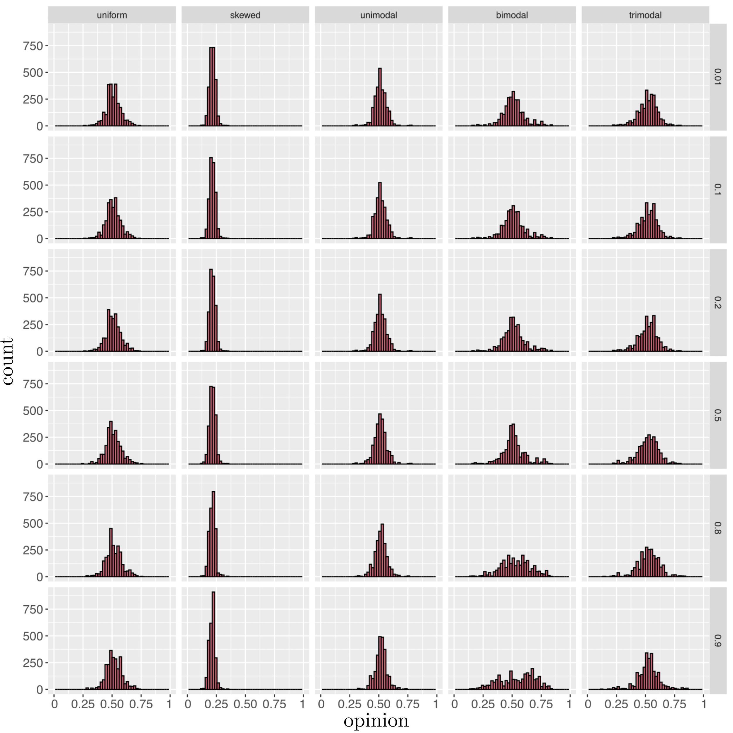
Figure 8: Limit opinion distributions of our weighted median model presented in Section 2.2 for our WS network for several initial opinion distributions and self-appraisal values. Each column has the same initial opinion distribution, and each row has the same self-appraisal value. The limit opinion distributions in each column are qualitatively similar to each other, so it seems that the self-appraisal value has little effect on the limit opinion distribution for our WS network.

Figure 9: Limit opinion distributions of our weighted median model presented in Section 2.2 for the Georgetown Facebook friendship network for several initial opinion distributions and self-appraisal values. Each column has the same initial opinion distribution, and each row has the same self-appraisal value. The limit opinion distributions in each column are qualitatively similar to each other, so it seems that the self-appraisal value has little effect on the limit opinion distribution for the Georgetown Facebook friendship network.

A.2 Summary statistics for the opinion-cluster sizes of the limit opinion distribution

In Tables 2–10, we give summary statistics for the opinion-cluster sizes of the limit opinion distribution of our weighted-median model presented in Section 2.2 for the networks in Section 3.2.

Statistic	Uniform	Unimodal	Skewed	Bimodal	Trimodal
Number of opinion clusters	1019	986	999	992	988
Mean size	2.51	2.48	2.54	2.53	2.54
Variance of the size	0.45	0.53	0.50	0.54	0.53
Kurtosis of the size	0.90	1.09	1.05	1.16	1.09

Table 2: Summary statistics for the opinion clusters of the limit opinion distribution of our weighted median model presented in Section 2.2 with self-appraisal $s=0.7$ for a 2500-node cycle network with several initial opinion distributions. For each initial opinion distribution, we performed a single simulation until the convergence criteria (3) was satisfied

.

Statistic	Uniform	Unimodal	Skewed	Bimodal	Trimodal
Number of opinion clusters	925	941	946	917	919
Mean size	2.70	2.66	2.64	2.72	2.72
Variance of the size	0.98	1.00	0.97	1.08	1.05
Kurtosis of the size	2.12	2.78	2.43	3.29	2.39

Table 3: Summary statistics for the opinion clusters of the limit opinion distribution of our weighted median model presented in Section 2.2 with self-appraisal $s=0.7$ for the 2500-node prism network with several initial opinion distributions. For each initial opinion distribution, we performed a single simulation until the convergence criteria (3) was satisfied.

Statistic	Uniform	Unimodal	Skewed	Bimodal	Trimodal
Number of opinion clusters	783	785	779	800	792
Mean size	3.19	3.18	3.21	3.13	3.16
Variance of the size	2.49	2.44	2.48	1.91	2.44
Kurtosis of the size	55.15	46.74	45.03	26.59	52.92

Table 4: Summary statistics for the opinion clusters of the limit opinion distribution of our weighted median model presented in section Section 2.2 with self-appraisal $s=0.7$ for the 2500-node square-lattice network with several initial opinion distributions. For each initial opinion distribution, we performed a single simulation until the convergence criteria (3) was satisfied.

Statistic	Uniform	Unimodal	Skewed	Bimodal	Trimodal
Number of opinion clusters	395	393	378	375	415
Mean size	6.32	6.36	6.61	6.67	6.02
Variance of the size	25.57	24.95	27.12	24.73	20.57
Kurtosis of the size	1.32$\times\,10^{4}$	1.52$\times\,10^{4}$	1.21$\times\,10^{4}$	5.70$\times\,10^{3}$	1.14$\times\,10^{4}$

Table 5: Summary statistics for the opinion clusters of the limit opinion distribution of our weighted median model presented in Section 2.2 with self-appraisal $s=0.7$ for a 2500-node WS network with several initial opinion distributions. For each initial opinion distribution, we performed a single simulation until the convergence criteria (3) was satisfied.

Statistic	Uniform	Unimodal	Skewed	Bimodal	Trimodal
Number of opinion clusters	43	40	57	41	47
Mean size	58.14	62.50	43.86	60.98	53.19
Variance of the size	8.09 $\times\,10^{4}$	8.88 $\times\,10^{4}$	6.32 $\times\,10^{4}$	8.57 $\times\,10^{4}$	8.90 $\times\,10^{4}$
Kurtosis of the size	2.63$\times\,10^{11}$	2.93$\times\,10^{11}$	2.17$\times\,10^{11}$	2.81$\times\,10^{11}$	3.54$\times\,10^{11}$

Table 6: Summary statistics for the opinion clusters of the limit opinion distribution of our weighted median model presented in Section 2.2 with self-appraisal $s=0.7$ for a 2500-node BA network with several initial opinion distributions. For each initial opinion distribution, we performed a single simulation until the convergence criteria (3) was satisfied.

Statistic	Uniform	Unimodal	Skewed	Bimodal	Trimodal
Number of opinion clusters	90	58	210	266	78
Mean size	8.47	13.14	3.6285	2.86	9.77
Variance of the size	3685.45	5117.64	29.05	11.05	3612.15
Kurtosis of the size	1.19$\times\,10^{9}$	1.44$\times\,10^{9}$	3.15$\times\,10^{4}$	2048.04	9.11$\times\,10^{8}$

Table 7: Summary statistics for the opinion clusters of the limit opinion distributions of our weighted median model presented in Section 2.2 with self-appraisal $s=0.7$ for the Caltech Facebook friendship network with several initial opinion distributions. For each initial opinion distribution, we performed a single simulation until the convergence criteria (3) was satisfied.

Statistic	Uniform	Unimodal	Skewed	Bimodal	Trimodal
Number of opinion clusters	289	1417	248	332	1185
Mean size	7.7854	1.5878	9.574	6.7771	1.8987
Variance of the size	6684.79	2.3467	7694.07	1253.13	79.14
Kurtosis of the size	1.27$\times\,10^{10}$	235.37	1.29$\times\,10^{10}$	2.55$\times\,10^{7}$	5.40$\times\,10^{6}$

Table 8: Summary statistics for the opinion clusters of the limit opinion distributions of our weighted median model presented in Section 2.2 with self-appraisal $s=0.7$ for the Bowdoin Facebook friendship network with several initial opinion distributions. For each initial opinion distribution, we performed a single simulation until the convergence criteria (3) was satisfied.

Statistic	Uniform	Unimodal	Skewed	Bimodal	Trimodal
Number of opinion clusters	2516	3686	3629	5303	4151
Mean size	3.73	2.55	2.59	1.77	2.26
Variance of the size	1365.86	201.77	101.26	287.42	497.17
Kurtosis of the size	2.20$\times\,10^{9}$	6.24$\times\,10^{8}$	1.43$\times\,10^{9}$	3.83$\times\,10^{8}$	6.07$\times\,10^{8}$

Table 9: Summary statistics for the opinion clusters of the limit opinion distribution of our weighted median model presented in Section 2.2 with self-appraisal $s=0.7$ for the Georgetown Facebook friendship network with several initial opinion distributions. For each initial opinion distribution, we performed a single simulation until the convergence criteria (3) was satisfied.

Statistic	Uniform	Unimodal	Skewed	Bimodal	Trimodal
Number of opinion clusters	1417	4414	3472	1539	2508
Mean size	5.65	2.81	2.31	5.20	3.19
Variance of the size	1.29$\times\,10^{4}$	3.11	53.02	3191.15	199.22
Kurtosis of the size	1.73$\times\,10^{12}$	516.61	1.81$\times\,10^{7}$	4.90$\times\,10^{10}$	2.52$\times\,10^{8}$

Table 10: Summary statistics for the opinion clusters of the limit opinion distribution of our weighted median model presented in Section 2.2 with self-appraisal $s=0.7$ for the Obamacare Twitter followership network with several initial opinion distributions. For each initial opinion distribution, we performed a single simulation until the convergence criteria (3) was satisfied.

Statistic	Uniform	Unimodal	Skewed	Bimodal	Trimodal
Number of opinion clusters	1123	1007	1044	1025	1077
Mean size	5.44	6.07	5.86	5.96	5.68
Variance of the size	5594.65	1.09 $\times\,10^{5}$	9837.41	1.26 $\times\,10^{4}$	9939.84
Kurtosis of the size	2.06$\times\,10^{10}$	8.95$\times\,10^{10}$	8.40$\times\,10^{11}$	1.44$\times\,10^{11}$	8.56$\times 10^{10}$

Table 11: Summary statistics for the opinion clusters of the limit opinion distributions of our weighted median model presented in Section 2.2 with self-appraisal $s=0.7$ for the abortion Twitter followership network with several initial opinion distributions. For each initial opinion distribution, we performed a single simulation until the convergence criteria (3) was satisfied.

Appendix B Mean-field approximation

In this appendix, we derive the mean-field approximation (6), present the specifications of our tests of its accuracy, and discuss issues that we encountered when numerically solving (6).

B.1 Derivation of our mean-field approximation (6)

We develop a degree-based mean-field approximation of our weighted-median model as presented in Section 2.2 for configuration-model networks with a prescribed degree distribution [16]. A degree-$k$ node has an associated opinion distribution $P_{k}(x,t)$ at time $t$. With our mean-field assumptions, which are inspired by the ones in [13], we derive a coupled system of difference equations for the time evolution of $P_{k}(x,t)$.

In our derivation, we make two key assumptions. First, we make an annealed-network assumption by rewiring the edges of the configuration-model network at each time step while fixing the network’s degree sequence [11]. Therefore, the network at each time step is one instantiation of our configuration-model ensemble. Second, we disregard the edge weights and edge directions.

Because we disregard edge weights and directions, at any time $t\in\mathbb{N}_{0}=\{0,\,1,\,\ldots\}$, our network $G=(V,E)$ is characterized by an unweighted and symmetric adjacency matrix $W$, where $W_{ij}=1$ if $(i,j)\in E$ and $W_{ij}=0$ otherwise. In contrast to an influence matrix (see Section 2.1), an adjacency matrix is not row-stochastic in general. We assume that the network $G$ has no isolated nodes.

Given an adjacency matrix $W$ of an undirected and unweighted network $G$, let $n(i)$ denote the number of neighbors of node $i$. Let $x_{i}(t)\in[0,1]$ for $i\in V$ be the opinion of individual $i$ at time $t\in\mathbb{N}_{0}$, and let the state $x(t)=(x_{1}(t),x_{2}(t),\ldots,x_{N}(t))$ be the vector of the $N$ node opinions. Given an initial state $x(0)$, our weighted-median model is the map

(7) $$x_{i}(t+1)=(1-s)x_{i}(t)+s\,\mathrm{Med}_{i}(x(t)\,;\,W)\,,\quad i\in V\,,$$

where $s\in(0,1)$ is the level of self-appraisal and $\mathrm{Med}_{i}(x(t)\,;\,W)$ is the median neighbor, which is the unique element of the set

(8) $$\left\{x_{k}\in x(t)\>\>\Big{|}\>W_{i\,k}=1\,,\>|\{j\,:x_{j}<x_{i}\}|\leq\frac{n(i)}{2}\,,\quad|\{j\,:x_{j}>x_{i}\}|\leq\frac{n(i)}{2}\,\right\}$$

that either minimizes the distance between $x_{k}(t)$ and $x_{i}(t)$ or is the numerically smaller value of the two if here are two elements in the set Eq. 8 with the same distance to $x_{i}(t)$. The network $G$ does not have to be connected; if $G$ has multiple components, then node opinions evolve independently on each component. However, we assume that $G$ is connected for convenience. One can view the weighted median model in Section 2.2 of the main text as a generalization of the above model because it allows for weighted edges.

Let $q_{k}$ denote the probability that a node of $G$ that we select uniformly at random has degree $k\in\mathbb{N}_{0}$. By assumption, there are no isolated nodes, so $q_{0}=0$. Let $D$ be the set of distinct degrees of the nodes. For each $k$, let $P_{k}(x,t)$ be the distribution of the opinions of degree-$k$ nodes at time $t$. The probability that a degree-$k$ node’s opinion is in the interval $[x,\,x+\Delta x)$ at time $t\in\mathbb{N}_{0}$ is thus $P_{k}(x,t)\Delta x+\mathcal{O}((\Delta x)^{2})$.

We derive a system of coupled finite-difference equations for the evolution of the densities $P_{k}(x,t)$ for $k\in D$. For large $N$ and small $\Delta x>0$, the expected number of degree-$k$ nodes with opinions in the interval $[x,\,x+\Delta x)$ is $Nq_{k}\,P_{k}(x,t)\Delta x$ at time $t$. The expected change of this number from time $t$ to time $t+1$ is

(9) $$Nq_{k}\,P_{k}(x,t+1)\Delta x-Nq_{k}\,P_{k}(x,t)\Delta x\,.$$

To obtain an expression for $P_{k}(x,t+1)$ as a function of $P_{k}(x,t)$, we derive an alternative form of the expected values in (9). We structure our derivations as follows. First, we derive the distribution of the opinion of a single neighbor of a degree-$k$ node. We then derive the distribution of the weighted-median opinion of the neighbors of a degree-$k$ node. From this latter quantity, we derive the mean number of opinions of degree-$k$ nodes that enter the interval $[x,\,x+\Delta x)$ at time $t+1$ and the mean number of opinions of degree-$k$ nodes that leave the interval $[x,\,x+\Delta x)$ at time $t+1$.

B.1.1 Opinion distribution of a uniformly random neighboring node

We now derive the opinion distribution of a uniformly random neighbor of a degree-$k$ node. Because the opinions evolve on a configuration-model network, the probability that a given edge that is incident to a degree-$k$ node is also incident to a specific degree-$l$ node is $\frac{l}{2|E|-1}$. As $N\rightarrow\infty$, the expected number of degree-$l$ nodes is approximately $2\frac{q_{l}|E|}{\sum_{i\in D}i\,q_{i}}$, where $\sum_{i\in D}i\,q_{i}$ is the mean degree. Therefore, as $N\rightarrow\infty$, the probability that a given edge that is incident to a degree-$k$ node is also incident to any degree-$l$ node is

(10) $$\pi_{l}=\frac{l\,q_{l}}{\langle d\rangle}\,,$$

which is independent of $k$.

We now derive the opinion distribution of a uniformly random neighbor of a node, which can have any degree. Because we randomly assign edges at each time step, the probability of a node being adjacent to a degree-$l$ node is independent of the node opinions in the asymptotic limit $N\rightarrow\infty$. The probability of a uniformly random neighbor having an opinion in the interval $[x,\,x+\Delta x)$ is

$$\mathbb{P}(x_{j}(t)\in[x,\,x+\Delta x)\,\cap\,e=(i,j)\in E\>|\>i,\,j\in V)$$

(11) $$=\sum_{l\in D}\mathbb{P}(\text{there is an edge between node $i$ and a degree-$l$ node})\,P_{l}(x,t)\Delta x$$

$$=\sum_{l\in D}\pi_{l}P_{l}(x,t)\Delta x$$

$$=\phi(x,t)\Delta x\,,$$

where $\phi(x,t)=\sum_{l\in D}\pi_{l}P_{l}(x,t)$ is the asymptotic opinion distribution of a uniformly random neighbor of any node as $N\rightarrow\infty$ and $D$ is the set of distinct degrees. Let $\Phi(x,t)=\int_{0}^{x}\phi(u,t)\,\mathrm{d}u$ denote the associated cumulative distribution function.

B.1.2 Distribution of the weighted-median opinion of neighboring nodes

Using equation (B.1.1), we derive the distribution of the median opinion of the neighbors of a degree-$k$ node. To do this, we introduce some notation and results for order statistics.

Order statistics

Suppose that $X_{1},X_{2},\ldots,X_{k}$ are independent univariate random variables with a common continuous probability density function $f_{X}$ and associated cumulative distribution function $F_{X}$. We order these random variables from smallest to largest. The $r$th order statistic $X_{(r)}$ has the probability density function [9]

(12) $$f_{X_{(r)}}(x)=\frac{n!}{(r-1)!(n-r)!}f_{X}(x)\left(F_{X}(x)\right)^{r-1}\left(1-F_{x}(x)\right)^{n-r}\,.$$

The conditional distribution of the $(r+1)$th order statistic given the $r$th order statistic is [9]

(13) $$f_{\{X_{(r+1)}|X_{(r)}=\,x\}}\,(y)=(n-r)\frac{f_{X}(y)}{1-F_{X}(x)}\left(\frac{1-F(y)}{1-F(x)}\right)^{n-r-1}.$$

Distribution of the weighted-median opinion of neighboring nodes

We now derive the distribution of the median opinion of neighboring nodes in a configuration-model network. Let node $i$ have degree $k$. We use separate arguments for odd and even $k$.

First, we consider odd $k$. Let $k=2m+1$. Because the opinions of the neighbors of node $i$ have the common distribution $\phi(x,t)$ as asymptotically $N\rightarrow\infty$, we view them as independent and identically distributed random variables. The median opinion $\mathrm{Med}_{i}(x,A)$ is the $(m+1)$th order statistic. It has the distribution

(14) $$\phi_{x_{(m+1)_{i}}}(x,t)=\frac{k!}{m!m!}\phi_{k}(x,t)\Phi_{k}(x,t)^{m}\left(1-\Phi(x,t)\right)^{m}\,.$$

Let $\theta_{k}(x,t)$ be the distribution of the median neighbor opinion of a node with degree $k$. For odd $k$, we can then write

(15) $$\theta_{k}(x,t)=\frac{k!}{m!m!}\phi_{k}(x,t)\Phi_{k}(x,t)^{m}\left(1-\Phi(x,t)\right)^{m}\,.$$

We now consider even $k$. Let $k=2m$. The quantity $\mathrm{Med}_{i}(x(t)\,;\,A)$ is either the $m$th or $(m+1)$th order statistic, depending on which of them is closer to $x_{i}(t)$. Given the definition of the weighted median in (8), we choose it to be the $m$th order statistic if they are equally close. Let $x_{(m)_{i}}$ and $x_{(m+1)_{i}}$, respectively, be the $m$th and $(m+1)$th order statistics of the opinions of the $k$ neighbors of node $i$.

In the asymptotic limit $N\rightarrow\infty$, the neighbor opinions have a common distribution $\phi(x,t)$. We derive an expression for the probability

(16) $$\mathbb{P}(\mathrm{Med}_{i}(x(t)\,;\,A)=x_{(m+1)_{i}}) =\mathbb{P}\left(\,|x_{i}-x_{(m+1)_{i}}|<|x_{i}-x_{(m)_{i}}|\right)\,,$$

where the opinion $x_{i}$ has the distribution $P_{k}(x,t)$.

If $x_{i}<x_{(m)_{i}}$, then the probability in (16) is $0$ because the $(m+1)$th order statistic is larger than $x_{(m)_{i}}$.

Assume that $x_{i}\geq x_{(m)_{i}}$ and let $c=x_{i}-x_{(m)_{i}}$. Equation (16) gives the probability that the $(m+1)$th order statistic is in the interval $[x_{(m)_{i}},x_{(m)_{i}}+2c)$. Using the law of total probability [35], we then write

(17) $$\mathbb{P}(\mathrm{Med}_{i}(x(t)\,;\,A)=x_{(m+1)_{i}})=$$

$$\hskip 14.22636pt\int_{x_{i}\in[0,1]}\int_{x_{(m)_{i}}\leq x_{i}}\int_{y\in[x_{(m)_{i}},-x_{(m)_{i}}+2x_{i})}\phi_{\{x_{(m+1)_{i}}|x_{(m)_{i}}\}}(y,t)\,P_{k}(x_{i},t)\,\phi_{x_{(m)_{i}}}(x_{(m)_{i}},t)\,\mathrm{d}y\,\mathrm{d}x_{(m)_{i}}\,\mathrm{d}x_{i}\,,$$

where $\phi_{\{x_{(m+1)_{i}}|x_{(m)_{i}}\}}$ is the distribution of the $(m+1)$th order statistic conditioned on the $m$th order statistic. Additionally, $[x_{(m)_{i}},\,x_{(m)_{i}}+2c)\,=[x_{(m)_{i}},\,-x_{(m)_{i}}+2x_{i})$. From equations (12) and (13), we see that

$$\phi_{\{x_{(m+1)_{i}}|x_{(m)_{i}}\}}(y,t) =m\frac{\phi(y)}{1-\Phi(x_{(m)_{i}},t)}\left(\frac{1-\Phi(y,t)}{1-\Phi(x_{(m)_{i}},t)}\right)^{m-1}\,,$$

$$\phi_{x_{(m)_{i}}}(b,t) =\frac{k!}{(m-1)!m!}\phi(b,t)\left(\Phi(b,t)\right)^{m-1}\left(1-\Phi(b,t)\right)^{m}$$

for $y\geq b$. Therefore,

$$\mathbb{P}(\mathrm{Med}_{i}(x(t)\,;\,A)=x_{(m+1)_{i}}) =\int_{x_{i}\in[0,1]}\int_{x_{(m)_{i}}\leq x_{i}}\int_{y\in[x_{(m)_{i}},-x_{(m)_{i}}+2x_{i})}m\frac{\phi(y,t)}{1-\Phi(x_{(m)_{i}},t)}\left(\frac{1-\Phi(y,t)}{1-\Phi(x_{(m)_{i}},t)}\right)^{m-1}$$

$$\qquad\qquad\quad\quad\quad\quad\quad\quad\times\frac{k!}{(m-1)!m!}\phi(x_{(m)_{i}},t)\left(\Phi(x_{(m)_{i}},t)\right)^{m-1}\left(1-\Phi(x_{(m)_{i}},t)\right)^{m}$$

$$\qquad\qquad\quad\quad\quad\quad\quad\quad\times P_{k}(x_{i},t)\,\mathrm{d}y\,\mathrm{d}x_{(m)_{i}}\,\mathrm{d}a$$

$$=\frac{k!}{((m-1)!)^{2}}\int_{x_{i}\in[0,1]}P_{k}(x_{i},t)\int_{x_{(m)_{i}}\leq x_{i}}\phi(x_{(m)_{i}},t)\left(\Phi(x_{(m)_{i}},t)\right)^{m-1}$$

$$\qquad\qquad\quad\quad\quad\quad\quad\quad\times\int_{y\in[x_{(m)_{i}},-x_{(m)_{i}}+2x_{i})}\phi(y,t)\left(1-\Phi(y,t)\right)^{m-1}\,\mathrm{d}y\,\mathrm{d}x_{(m)_{i}}\,\mathrm{d}x_{i}\,.$$

We define the notation $p_{k}(t)=\mathbb{P}(\mathrm{Med}_{i}(x(t)\,;\,A)=x_{(m+1)_{i}})$, and we express $\theta_{k}$ using the $m$th and $(m+1)$th order statistics of $\phi(x,t)$. For $k=2m$, we have

$$\theta_{k}(x,t) =(1-p(t))\phi_{x_{(m)}}(x,t)+p(t)\phi_{x_{(m+1)}}(x,t)$$

$$=(1-p_{k}(t))\frac{k!}{(m-1)!m!}\phi(x,t)\Phi(x,t)^{m-1}\left(1-\Phi(x,t)\right)^{m}$$

$$\qquad+p_{k}(t)\frac{k!}{(m-1)!m!}\phi(x,t)\Phi(x,t)^{m}\left(1-\Phi(x,t)\right)^{m-1}$$

(18) $$=\frac{k!}{(m-1)!m!}\phi(x,t)\big{(}\Phi(x,t)\left(1-\Phi(x,t)\right)\big{)}^{m-1}$$

$$\hskip 56.9055pt\times\big{(}(1-p_{k}(t))\left(1-\Phi(x,t)\right)+p_{k}(t)\Phi(x,t)\big{)}\,.$$

From equations (15) and (B.1.2), we see that the median neighbor opinion of a degree-$k$ node has the distribution

(19) $$\theta_{k}(x,t)=\begin{cases}\frac{k!}{m!m!}\phi_{k}(x,t)\Phi_{k}(x,t)^{m}\left(1-\Phi(x,t)\right)^{m}\,,\qquad\text{$k=2m+1$}\\ \begin{array}[]{l}\frac{k!}{(m-1)!m!}\phi(x,t)\big{(}\Phi(x,t)\left(1-\Phi(x,t)\right)\big{)}^{m-1}\\ \hskip 14.22636pt\times\big{(}(1-p(t))\left(1-\Phi(x,t)\right)+p(t)\Phi(x,t)\big{)}\end{array}\,,\qquad\text{$k=2m$}\,,\end{cases}$$

where

$$p_{k}(t) =\frac{k!}{((m-1)!)^{2}}\int_{a\in[0,1]}P_{k}(x_{i},t)\int_{b\leq x_{i}}\phi(b,t)\left(\Phi(b,t)\right)^{m-1}$$

(20) $$\quad\quad\quad\quad\quad\quad\quad\quad\quad\quad\quad\times\int_{y\in[b,-b+2x_{i})}\phi(y,t)\left(1-\Phi(y,t)\right)^{m-1}\,\mathrm{d}y\,\mathrm{d}b\,\mathrm{d}x_{i}\,.$$

B.1.3 Mean number of degree-$k$ nodes with opinions that enter the interval $[x,\,x+\Delta x)$ at time $t+1$

Using (19), we derive the expected number of nodes whose opinions are outside the interval $[x,\,x+\Delta x)$ at time $t$ but inside this interval at time $t+1$. Let $i\in V$ be a degree-$k$ node, and suppose that $x_{i}(t)=y\notin[x,\,x+\Delta x)$. For the opinion of node $i$ to enter $[x,\,x+\Delta x)$, it must be the case that

(21) $$x\leq(1-s)y+s\,\mathrm{Med}_{i}(x(t),A)<x+\Delta x\,,$$

which yields

(22) $$\frac{x+(s-1)y}{s}\leq\mathrm{Med}_{i} (x(t),A)<\frac{x+(s-1)y}{s}+\frac{\Delta x}{s}$$

for $s\neq 0$.

Because node $i$ has degree $k$, we know that $\mathrm{Med}_{i}(x(t);\,A)$ has the distribution $\theta_{k}(x,t)$ asymptotically as $N\rightarrow\infty$. The probability that (21) holds is thus

(23) $$\theta_{k}\left(\frac{x+(s-1)y}{s},t\right)\frac{\Delta x}{s}\,.$$

The expected number of degree-$k$ nodes that at time $t$ have an opinion in $[y,\,y+\mathrm{d}y)$ but outside $[x,\,x+\Delta x)$ and then at time $t+1$ have an opinion in $[x,\,x+\Delta x)$ is approximately

(24) $$\frac{Nq_{k}}{s}\theta_{k}\left(\frac{x+(s-1)y}{s},t\right)\frac{\Delta x}{s}P_{k}(y,t)\Delta x\,\mathrm{d}y\,.$$

The approximate nature of our statement arises because the intervals $[x,\,x+\Delta x)$ and $[y,\,y+\mathrm{d}y)$ may overlap. However, this overlap disappears as $\Delta x\rightarrow 0$ and $\mathrm{d}y\rightarrow 0$. Integrating over $y$, we see that the mean number of degree-$k$ nodes whose opinions enter $[x,\,x+\Delta x)$ at time $t+1$ is

(25) $$Nq_{k}\int_{y\in[0,1]}\theta_{k}\left(\frac{x+(s-1)y}{s},t\right)\frac{\Delta x}{s}P_{k}(y,t)\Delta x\,\mathrm{d}y\,.$$

B.1.4 Expected number of degree-$k$ nodes with opinions that leave interval $[x,\,x+\Delta x)$ at time $t+1$

We now consider the mean number of degree-$k$ nodes whose opinion is in $[x,\,x+\Delta x)$ at time $t$ but not at time $t+1$. We argue similarly as in Section B.1.3, although now our argument is a bit simpler. Because the opinion of a degree-$k$ node follows the distribution $P_{k}(x,t)$ and the weighted median of its neighbors’ opinions has the distribution $\theta_{k}(x,t)$ asymptotically as $N\rightarrow\infty$, the probability that $x_{i}(t)\in[x,\,x+\Delta x)$ and $x_{i}(t+1)\notin[x,\,x+\Delta x)$ is asymptotically

(26) $$\left(1-\theta_{k}(x,t)\Delta x\right)P_{k}(x,t)\Delta x\,.$$

The mean number of such nodes is thus

(27) $$Nq_{k}\left(1-\theta_{k}(x,t)\Delta x\right)P_{k}(x,t)\Delta x\,.$$

B.1.5 Expected change in the number of degree-$k$ nodes with opinions in the interval $[x,\,x+\Delta x)$ at time $t+1$

Combining equations (9), (25), and (27) yields

(28) $$Nq_{k}\,P_{k}(x,t+1)\Delta x-Nq_{k}\,P_{k}(x,t)\Delta x$$

$$\qquad=Nq_{k}\int_{y\in[0,1]}\theta_{k}\left(\frac{x+(s-1)y}{s},t\right)\frac{\Delta x}{s}P_{k}(y,t)\,\mathrm{d}y\Delta x-Nq_{k}\left(1-\theta_{k}(x,t)\Delta x\right)P_{k}(x,t)\Delta x\,\,,$$

which implies that

(29) $$P_{k}(x,t+1) \rightarrow\frac{1}{s}\int_{y\in[0,1]}\theta_{k}\left(\frac{x+(s-1)y}{s},t\right)P_{k}(y,t)\,\mathrm{d}y\quad\text{as}\quad\Delta x\rightarrow 0\,.$$

This finishes our derivation of the mean-field approximation (6).

B.2 Finite-size effects and inaccuracies from annealing-like effects

In our derivation of the mean-field approximation (6), we made two key assumptions: (1) we examined the $N\rightarrow\infty$ asymptotic regime and (2) we assumed that the dynamics occur on an annealed network [11]. Both of these choices affect the accuracy of our approximation.

We now examine finite-size effects (i.e., inaccuracies that arise from our asymptotic assumption) and annealing-assumption effects (i.e., inaccuracies that arise from the annealed-network assumption) in our mean-field approximation.

We observe both finite-size effects and annealing-assumption effects, but they seem to diminish quickly with time for most values of self-appraisal. Both finite-size effects and annealing-assumption effects are dominated by the impact of self-appraisal on the accuracy of our mean-field approximation.

To examine finite-size effects, we calculate the root-mean-square error (RMSE) of numerical solutions to our mean-field approximation when compared to ensemble averages of simulations of our weighted median model presented in Section 2.2 for several network sizes $N$.

To examine annealing-assumption effects, we calculate ensemble averages of simulations for our weighted-median for two types of networks: static and annealing configuration-model networks.

The static networks are sampled from a $(k_{1},\,k_{2})$-regular configuration-model with degrees $k_{1}=11$, $k_{2}=101$, and associated probabilities $q_{k_{1}}=0.9$ and $q_{k_{2}}=0.1$. After the initial instantiation of the static network, it does not change during the simulation of our weighted median model. The annealing networks are also $(k_{1},\,k_{2})$-regular configuration-model networks with the same values of $k_{1}$ and $k_{2}$ as the static networks and the same associated probabilities. However, after the initial instantiation, at each time step of the simulation, the edges of the annealing networks are rewired randomly while preserving their degree sequences. Therefore, the annealing networks satisfy the annealing-network assumption made in the derivation of the mean-field approximation (6) while the static networks do not.

We show the RMSE of these numerical experiments in Fig. 10 where time moves from top ($t=1$) to bottom ($t=5$). At time $t=1$ and for all values of the self-appraisal $s$, the RMSE is smaller for larger networks for both the annealed and the static networks. Notably, network size seems to affect the RMSE more than the self-appraisal value. The RMSE has a similar magnitude for the static and annealing networks. This suggests that finite-size effects are impacting the accuracy of our mean-field approximation at time $t=1$ but that there are not any significant annealing-assumption effects.

At time $t=3$, the dependency between network size and the RMSE is less pronounced for both annealed and static networks. For annealed networks at time $t=3$, we also observe that the RMSE is smaller for larger networks, especially for small self-appraisals $s$. However, at time $t=3$ for static networks, this tendency is almost entirely absent, except for our simulations with self-appraisal $s=0.1$. For self-appraisal values below $0.9$, the RMSEs of the static networks are larger than for the annealed networks. Therefore, at time $t=3$, it seems that finite-size effects still impact the accuracy of our approximation and that effect of the the self-appraisal value and the annealing-assumption effects are more pronounced than for $t=1$.

At time $t=5$, the finite-size effects are still noticeable for the annealed networks for $s\leq 0.5$. For static networks at time $t=5$, we barely observe any noticeable finite-size effects. The RMSEs for static networks are larger than those for annealed networks for self-appraisals below $0.7$. However, at time $t=5$, the self-appraisal has a larger impact than either finite-size effects of annealing-assumption effects on the accuracy of our mean-field approximation.

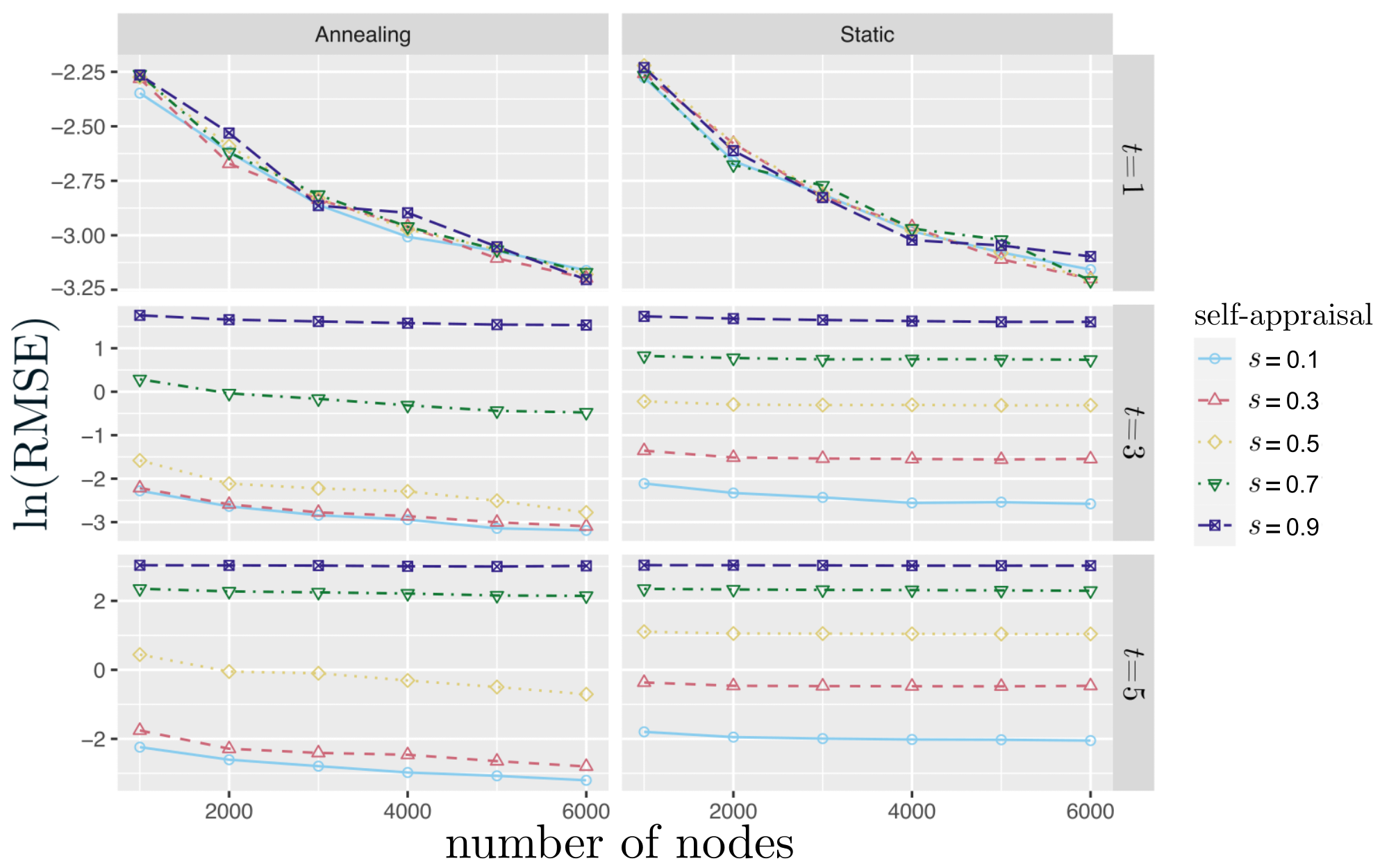
Figure 10: The natural logarithm of the RMSE of the mean-field approximation (6) for annealed and static networks that we generate using a $(k_{1},k_{2})$-regular configuration model with varying number of nodes. The static networks are sampled from a $(k_{1},\,k_{2})$-regular configuration-model with degrees $k_{1}=11$, $k_{2}=101$, and associated probabilities $q_{k_{1}}=0.9$ and $q_{k_{2}}=0.1$. After the initial instantiation, static networks do not change during the simulation. The annealing networks are also $(k_{1},\,k_{2})$-regular configuration-model networks with the same values of $k_{1}$ and $k_{2}$ as the static networks and the same associated probabilities. However, after the initial instantiation, at each time step of the simulation, the edges of the annealing networks are rewired randomly while preserving their degree sequences. Therefore, the annealing networks satisfy the annealing assumption made in the derivation of the mean-field approximation, whereas the static networks do not. At time $t=1$, the RMSE is smaller for larger networks for all values of the self-appraisal $s$. However, at later times, the impact of network size diminishes. At time $t=5$, the effect of self-appraisal dominates both annealing-like and finite-size effects.

B.3 Effects of self-appraisal on root-mean-square error (RMSE) of the mean-field approximation (6)

In Fig. 11, we show the dependency of the RMSE of the mean-field approximation (6) for the Bowdoin Facebook friendship network using a more finely-gained set of self-appraisal values than the one that we used in section 4.1. For self-appraisal $s=0.1$, the RMSE initially increases rapidly, and it then increases slowly for $t\geq 1$. For $s=0.3$, the RMSE initially increases slowly, and it then increases much more rapidly. We examine self-appraisal values that lie between these extremes and observe a seemingly smooth transition between these two behaviors. We observe similar qualitative features for our other real-world social networks.

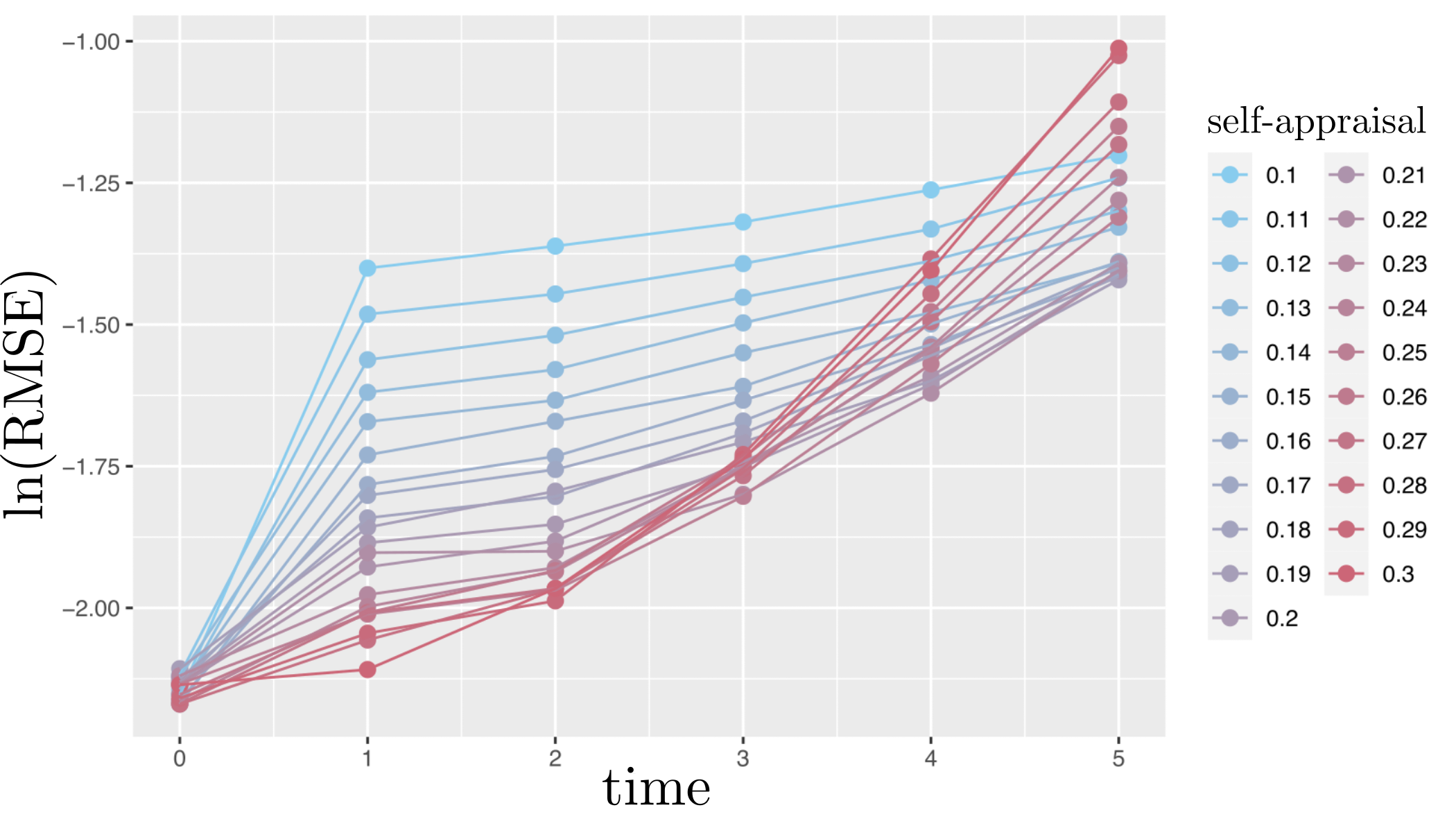
Figure 11: The natural logarithm of the RMSE of the mean-field approximation (6) for the Bowdoin Facebook friendship network for values of self-appraisal between $s=0.1$ and $s=0.3$. The RMSE increases rapidly at earlier times for self-appraisal values near $0.1$ than it does for self-appraisal values near $0.3$. There appears to be a smooth transition between these two behaviors.

B.4 Effect of degree “lumping” on the RMSE of the mean-field approximation (6)

We found in Section 4.1 that the maximum value of $\theta_{k}$ in our mean-field approximation (6) increases with the node degree $k$. This results in numerical overflow in the evaluation of $\theta_{k}$ for sufficiently large values of $k$; the function value of $\theta_{k}$ at the mode of the distribution exceeds the machine limits for floating-point numbers. To deal with this issue, we introduce a “lumping degree” and aggregate all degree-$k$ nodes when $k$ is at least some lumping degree into a single degree class with a common opinion distribution. The probability that a node is in the lumped degree class is the sum of the probabilities that it is any of its constituent degree classes.

Using numerical computations, we examine the effect of different lumping degrees on the mean-field approximation (6). In Fig. 12, we show the RMSE of the mean-field approximation for the Georgetown Facebook network at times $t=1$ and $t=4$ for different lumping degrees and self-appraisal values. The behavior of the RMSE depends on the self-appraisal $s$. At time $t=4$, for self-appraisal $s=0.1$, the RMSE initially decreases with the lumping degree. However, the RMSE initially increases with lumping degree for larger self-appraisal values.

In Fig. 13, we show the RMSE of the mean-field approximation for the Georgetown Facebook network at times $t=1$ and $t=4$ for different lumping degrees for self-appraisals $s\in[0.1,0.3]$. There appears to be a smooth transition between the observed behaviors.

Based on our simulations of our mean-field approximation (6) on our Facebook friendship and Twitter followership networks, there also appears to be little effect of increasing the lumping degree beyond $500$. For all of the results in section 6 of the main manuscript, we used a lumping degree of $1000$.

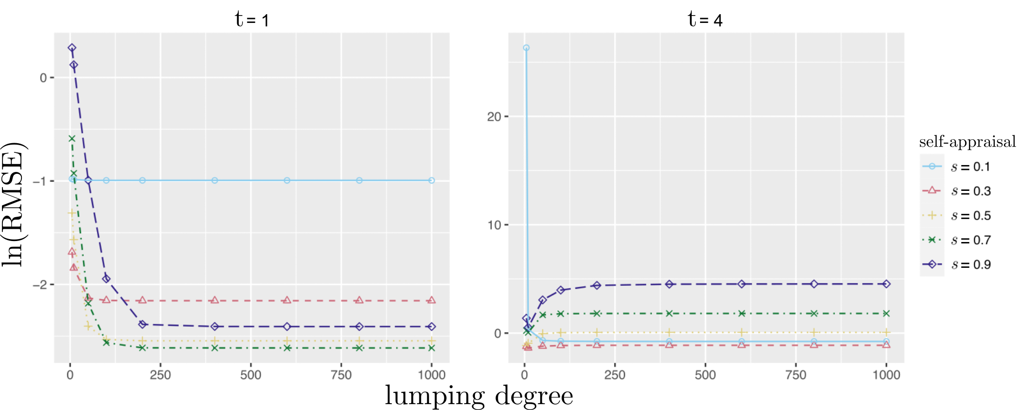
Figure 12: The natural logarithm of the RMSE of the mean-field approximation (6) for the Georgetown Facebook friendship network at times $t=1$ and $t=4$ for various lumping degrees and values of the self-appraisal $s$. The RMSE appears to be similar for lumping degrees of at least $500$. We observe this situation for all of our Facebook friendship networks and Twitter followership networks.

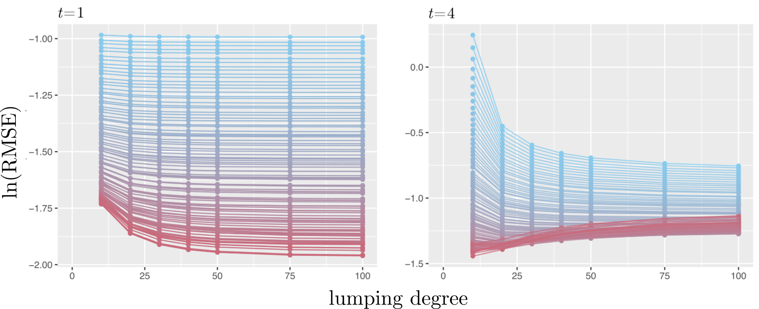
Figure 13: The natural logarithm of the RMSE of the mean-field approximation (6) for the Georgetown Facebook friendship network at times $t=1$ and $t=4$ for various lumping degrees and values of self-appraisal ranging from $s=0.1$ (light blue) to $s=0.3$ (red). The RMSE evolves differently for $s=0.1$ than it does for $s=0.3$. At $t=1$, the RMSE depends little on the lumping degree for $s=0.1$, but it decreases for larger lumping degrees for $s=0.3$. At $t=4$, the RMSE decreases for larger lumping degrees for $s=0.1$, but it increases for larger lumping degrees for $s=0.3$. There appears to be a smooth transition between these the two regimes.

References

- [1] M. Agranov, J. K. Goeree, J. Romero, and L. Yariv, What makes voters turn out: The effects of polls and beliefs, Journal of the European Economic Association, 16 (2017), pp. 825–856.
- [2] A. L. Barabási and R. Albert, Emergence of scaling in random networks, Science, 286 (1999), pp. 509–512.
- [3] J. W. Baron, Consensus, polarization, and coexistence in a continuous opinion dynamics model with quenched disorder, Physical Review E, 104 (2021), 044309.
- [4] R. K. Beasley and M. R. Joslyn, Cognitive dissonance and post-decision attitude change in six presidential elections, Political Psychology, 22 (2001), pp. 521–540.
- [5] J. Bedson, L. A. Skrip, D. Pedi, S. Abramowitz, S. Carter, M. F. Jalloh, S. Funk, N. Gobat, T. Giles-Vernick, G. Chowell, J. R. de Almeida, R. Elessawi, S. V. Scarpino, R. A. Hammond, S. Briand, J. M. Epstein, L. Hébert-Dufresne, and B. M. Althouse, A review and agenda for integrated disease models including social and behavioural factors, Nature Human Behaviour, 5 (2021), pp. 834–846.
- [6] C. Bernardo, C. Altafini, A. Proskurnikov, and F. Vasca, Bounded confidence opinion dynamics: A survey, Automatica, 159 (2024), 111302.
- [7] G. Biddlestone and K. M. Douglas, Cultural orientation, power, belief in conspiracy theories, and intentions to reduce the spread of COVID-19, British Journal of Social Psychology, 59 (2020), pp. 663–673.
- [8] H. Z. Brooks and M. A. Porter, A model for the influence of media on the ideology of content in online social networks, Physical Review Research, 2 (2020), 023041.
- [9] H. A. David and H. N. Nagaraja, Order Statistics, John Wiley & Sons, Inc., New York City, NY, USA, 3rd ed., 2003.
- [10] M. H. DeGroot, Reaching a consensus, Journal of the American Statistical Association, 69 (1974), pp. 118–121.
- [11] S. N. Dorogovtsev, A. V. Goltsev, and J. F. F. Mendes, Critical phenomena in complex networks, Reviews of Modern Physics, 80 (2008), pp. 1275–1335.
- [12] Eeti, A. Singh, and H. Cherifi, Centrality-based opinion modeling on temporal networks, IEEE Access, 8 (2020), pp. 1945–1961.
- [13] S. C. Fennell, K. Burke, M. Quayle, and J. P. Gleeson, Generalized mean-field approximation for the Deffuant opinion dynamics model on networks, Physical Review E, 103 (2021), 012314.
- [14] L. Festinger, A Theory of Cognitive Dissonance, Stanford University Press, Stanford, CA, USA, 1957.
- [15] L. Festinger and J. M. Carlsmith, Cognitive consequences of forced compliance, Journal of Abnormal and Social Psychology, 58 (1959), pp. 203–210.
- [16] B. Fosdick, D. Larremore, J. Nishimura, and J. Ugander, Configuring random graph models with fixed degree sequences, SIAM Review, 60 (2018), pp. 315–355.
- [17] K. Garimella, G. De Francisci Morales, A. Gionis, and M. Mathioudakis, Political discourse on social media: Echo chambers, gatekeepers, and the price of bipartisanship, in Proceedings of the 2018 World Wide Web Conference, WWW ’18, Republic and Canton of Geneva, Switzerland, 2018, pp. 913–922.
- [18] Y. Han, G. Chen, F. Dörfler, and W. Mei, The continuous-time weighted-median opinion dynamics, 2024, https://arxiv.org/abs/2404.16318.
- [19] A. Hickok, Y. Kureh, H. Z. Brooks, M. Feng, and M. A. Porter, A bounded-confidence model of opinion dynamics on hypergraphs, SIAM Journal on Applied Dynamical Systems, 21 (2022), pp. 1–32.
- [20] P. Jia, A. Mirtabatabaei, N. E. Friedkin, and F. Bullo, Opinion dynamics and the evolution of social power in influence networks, SIAM Review, 57 (2015), pp. 367–397.
- [21] P. F. Lazarsfeld, B. Berelson, and H. Gaudet, The People’s Choice. How the Voter Makes Up His Mind in a Presidential Campaign: Legacy edition, Columbia University Press, New York City, NY, USA, 2021.
- [22] F. J. León-Medina, J. Tena-Sánchez, and F. J. Miguel, Fakers becoming believers: How opinion dynamics are shaped by preference falsification, impression management and coherence heuristics, Quality & Quantity, 54 (2020), p. 385–412.
- [23] G. Li, Q. Liu, and L. Chai, Analysis and application of weighted-median hegselmann-krause opinion dynamics model on social networks, in 2022 34th Chinese Control and Decision Conference (CCDC), 2022, pp. 5409–5414, https://doi.org/10.1109/CCDC55256.2022.10033719.
- [24] J. Lorenz, Consensus strikes back in the Hegselmann–Krause model of continuous opinion dynamics under bounded confidence, Journal of Artificial Societies and Social Simulation, 9 (2006), 8.
- [25] J. Lorenz, Heterogeneous bounds of confidence: Meet, discuss and find consensus!, Complexity, 15 (2010), pp. 43–52.
- [26] J. Lorenz and D. A. Lorenz, On conditions for convergence to consensus, IEEE Transactions on Automatic Control, 55 (2010), pp. 1651–1656, https://doi.org/10.1109/TAC.2010.2046086.
- [27] D. C. Matz and W. Wood, Cognitive dissonance in groups: The consequences of disagreement, Journal of Personality and Social Psychology, 88 (2005), pp. 22–37.
- [28] M. Medo, M. S. Mariani, and L. Lü, The fragility of opinion formation in a complex world, Communications Physics, 4 (2021), 75.
- [29] W. Mei, F. Bullo, G. Chen, J. M. Hendrickx, and F. Dörfler, Micro-foundation of opinion dynamics: Rich consequences of the weighted-median mechanism, Physical Review Research, 4 (2022), 023213.
- [30] W. Mei, J. M. Hendrickx, G. Chen, F. Bullo, and F. Dörfler, Convergence, consensus and dissensus in the weighted-median opinion dynamics, IEEE Transactions on Automatic Control, (2024), pp. 1–15, https://doi.org/10.1109/TAC.2024.3376752.
- [31] S. Melnik, J. A. Ward, J. P. Gleeson, and M. A. Porter, Multi-stage complex contagions, Chaos, 23 (2013), 013124.
- [32] X. F. Meng, R. A. V. Gorder, and M. A. Porter, Opinion formation and distribution in a bounded-confidence model on various networks, Physical Review E, 97 (2018), 022312.
- [33] M. E. J. Newman, Networks, Oxford University Press, second ed., 2018.
- [34] H. Noorazar, K. R. Vixie, A. Talebanpour, and Y. Hu, From classical to modern opinion dynamics, International Journal of Modern Physics C, 31 (2020), 2050101.
- [35] J. Pitman, Probability, Springer-Verlag, Heidelberg, Germany, 1st ed., 1993.
- [36] M. A. Porter and J. P. Gleeson, Dynamical Systems on Networks: A Tutorial, vol. 4 of Frontiers in Applied Dynamical Systems: Reviews and Tutorials, Springer International Publishing, Cham, Switzerland, 2016.
- [37] S. Redner, Reality-inspired voter models: A mini-review, Comptes Rendus Physique, 20 (2019), pp. 275–292.
- [38] H. Schawe, S. Fontaine, and L. Hernández, When network bridges foster consensus. Bounded confidence models in networked societies, Physical Review Research, 3 (2021), 023208.
- [39] H. Schawe and L. Hernández, Higher order interactions destroy phase transitions in Deffuant opinion dynamics model, Communications Physics, 5 (2022), 32.
- [40] K. Sugishita, M. A. Porter, M. Beguerisse-Díaz, and N. Masuda, Opinion dynamics on tie-decay networks, Physical Review Research, 3 (2021), 023249.
- [41] A. L. Traud, P. J. Mucha, and M. A. Porter, Social structure of Facebook networks, Physica A: Statistical Mechanics and its Applications, 391 (2012), pp. 4165–4180.
- [42] D. J. Watts and S. H. Strogatz, Collective dynamics of ‘small-world’ networks, Nature, 393 (1998), pp. 440–442.
- [43] H. Xia, H. Wang, and Z. Xuan, Opinion dynamics: A multidisciplinary review and perspective on future research, International Journal of Knowledge and Systems Science, 2 (2011), pp. 72–91.
- [44] D. Zhaogang, C. Xia, D. Yucheng, and F. Herrera, Consensus reaching in social network DeGroot model: The roles of the self-confidence and node degree, Information Sciences, 486 (2019), pp. 62–72.