Accelerated creation of NOON states with ultracold atoms
via counterdiabatic driving

Abstract

A quantum control protocol is proposed for the creation of NOON states with N ultracold bosonic atoms on two modes, corresponding to the coherent superposition $|N,0\rangle+|0,N\rangle$. This state can be prepared by using a third mode where all bosons are initially placed and which is symmetrically coupled to the two other modes. Tuning the energy of this third mode across the energy level of the other modes allows the adiabatic creation of the NOON state. While this process normally takes too much time to be of practical usefulness, due to the smallness of the involved spectral gap, it can be drastically boosted through counterdiabatic driving which allows for efficient gap engineering. We demonstrate that this process can be implemented in terms of static parameter adaptations that are experimentally feasible with ultracold quantum gases. Gain factors in the required protocol speed are obtained that increase exponentially with the number of involved atoms and thus counterbalance the exponentially slow collective tunneling process underlying this adiabatic transition.

The concept of entanglement is of fundamental importance in quantum physics [1] and lies at the heart of various protocols in quantum information science [2]. A particularly intriguing category of entangled states are NOON states, given by a coherent superposition of the form $|N,0\rangle+e^{i\varphi}|0,N\rangle$ which involves $N$ bosons distributed over two modes. They can be seen as microscopic Schrödinger cat states and are of great potential interest in the context of quantum metrology [3, 4, 5, 6, 7] especially when being realized with massive bosons.

While NOON states with up to $N\sim 10$ quanta were already produced with photons and phonons [8, 9, 10], their experimental realization with ultracold bosonic atoms is yet to be achieved. Various strategies and protocols how to prepare such NOON states with bosonic quantum gases were proposed [11, 12, 13, 14, 15, 16, 17], using the intrinsic interaction between the atoms of the gas as a key ingredient. Indeed, rather than being a nuisance, the presence of atom-atom interaction can be pivotally exploited to facilitate the creation of the NOON superposition since the components $|N,0\rangle$ and $|0,N\rangle$ that form the latter can thus be energetically isolated within the system’s eigenspectrum.

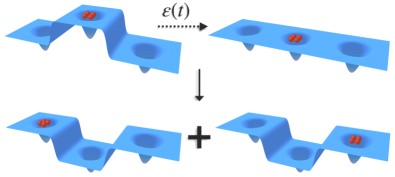
Figure 1: Schematic representation of the proposed protocol. Initially, all bosons are placed in a mode that is energetically at the top of the spectrum. Subsequently, the energy of this mode is lowered in order to achieve an avoided crossing with another energy level corresponding to the coherent superposition of the states $|N,0,0\rangle$ and $|0,0,N\rangle$. A NOON state $|N,0,0\rangle+|0,0,N\rangle$ is thus obtained at the end of this adiabatic transition process.

In particular, this allows one to generate a NOON state via collective tunneling [18, 19, 20, 21], in the parameter regime of macroscopic quantum self-trapping [22], namely by preparing the system in the state $|N,0\rangle$ and waiting half the time that it would take to tunnel to $|0,N\rangle$. Despite its appealing simplicity, this particular preparation protocol is not suited for experimental realization since the collective tunneling time is extremely long and increases exponentially with the particle number $N$. It was recently proposed [23] to expose the two-mode configuration to a properly tuned periodic driving, thus giving rise to chaos-assisted tunneling [24]. This procedure allows one to drastically enhance collective tunneling without appreciably affecting the purity of the resulting NOON superposition [23] and can be generalized to realize more exotic triple-NOON states on three modes [25]. However, it still suffers from a relatively long preparation time (of the order of a second for ultracold ⁸⁷Rb gases with $N=5$ [23]) and thus imposes great technical challenges concerning the maintaining of perfect symmetry between the involved single-particle modes as well as the shielding of the system against stray fields and noise effects.

To overcome the time scale problem, we employ here a different approach which is based on adiabatic transitions. To this end, we consider the presence of a third mode which is symmetrically coupled to the other two modes and has a tunable single-particle energy. Initially preparing all atoms on this third mode and tuning its energy sufficiently slowly across the energy of the other two modes allows one to induce an adiabatic transfer of the system’s state to the desired NOON superposition forming on the other two modes. While this process also requires a long realization time, which is inversely proportional to the spectral gap of the avoided level crossing, gap engineering techniques based on shortcuts to adiabaticity have been developed [26, 27, 28, 29, 30, 31] that can be exploited here to widen the gap. We show that an efficient counterdiabatic driving protocol can be implemented for this purpose. This protocol amounts to adaptations of the (interaction and hopping) parameters that characterize the many-body system, which are static if the protocol for the time-dependent tuning of the third mode’s energy is pre-optimized according to geodesic control [32, 33, 34, 35]. It is thus experimentally feasible and allows one to generate the NOON state with high fidelity on time scales that are drastically reduced as compared to collective tunneling.

Theoretical framework. Our system is theoretically described by a Bose-Hubbard model, which models $N$ bosonic atoms that are confined in a lattice with $L=3$ wells [36]. The atoms experience an interaction $U$ due to the presence of other atoms in the same well and can tunnel at a rate $J$ between different wells. For $L=3$, the Hamiltonian describing the system can be written as:

$$\hat{H}(t)= \frac{U}{2}\sum_{i=1}^{3}\hat{a}_{i}^{\dagger}\hat{a}_{i}^{\dagger}\hat{a}_{i}\hat{a}_{i}-J\sum_{i=1}^{2}\left(\hat{a}^{\dagger}_{i+1}\hat{a}_{i}+\hat{a}^{\dagger}_{i}\hat{a}_{i+1}\right)$$ (1)

$$+\varepsilon(t)\hat{a}_{2}^{\dagger}\hat{a}_{2},$$

where $\hat{a}_{i}^{\dagger}$ and $\hat{a}_{i}$ are the creation and annihilation operators for a bosonic particle at site $i$, respectively, and where we added a controlable time-dependent on-site energy $\varepsilon(t)$ for the central well.

This system exhibits a range of interesting phenomena depending on the values of the interaction and hopping parameters. When the interaction is sufficiently large compared to the tunneling rate between sites, the particles are completely localized in their respective sites, forming what is known as a Mott insulator, while a superfluid state can be achieved when the hopping is large enough relative to the interaction to allow particles to move freely between the sites [37]. The presence of interaction allows the many-body spectrum to be completely divided into multiple parts. In particular, states where all particles are in the same site are all localized at the top of the spectrum, isolated from the rest by a gap of size $\approx U(N-1)/J$. The presence of interaction is thus of crucial importance for our method, as it induces a gap-protected reduced system that is useful for engineering the NOON state creation.

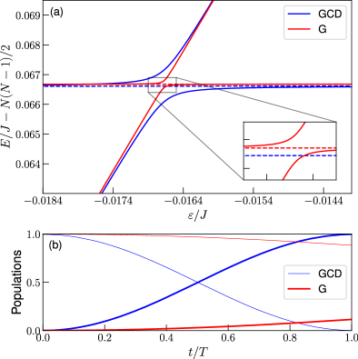
Figure 2: (a) Spectrum of the Hamiltonian as a function of the driving parameter $\varepsilon$, for $U=20J$, and $N=4$, focusing on the three relevant levels. The red curves correspond to the original driven Hamiltonian (G method), while the blue curves represent the modified spectrum obtained through our new GCD method for $T=10^{3}\hbar/J$, which combines an optimized driving protocol with the counterdiabatic Hamiltonian. Antisymmetric states are depicted with dashed lines. The inset shows the avoided crossing using only an optimized driving. (b) Detection probabilities for a fixed total protocol time $T=3\times 10^{3}\hbar/J$. Thick curves indicates the probability of finding the system in the state $\ket{NOON}$, while thin curves relates to the probability of measuring the state $\ket{0,N,0}$. One can observe a nearly perfect transition with the GCD method, in contrast to method G, which only attains around 10% of population inversion.

Due to the delocalization of states $|N,0,0\rangle$, $|0,N,0\rangle$ and $|0,0,N\rangle$, the dynamics of the system can be effectively described in terms of a 3-level system. The reduced Hamiltonian in the Fock basis $\mathcal{B}=\left\{|N,0,0\rangle,|0,N,0\rangle,|0,0,N\rangle\right\}$ is given by:

$$H_{\text{red}}(U,J,\varepsilon(t))=\left(\begin{tabular}[]{c c c}$\mathcal{E}$&$-\mathcal{J}$&0\\ $-\mathcal{J}$&$\tilde{\mathcal{E}}+\mathcal{N}\varepsilon(t)$&$-\mathcal{J}$\\ 0&$-\mathcal{J}$&$\mathcal{E}$\\ \end{tabular}\right)$$ (5)

where $\mathcal{E}=\mathcal{E}(U,J)$, $\tilde{\mathcal{E}}=\tilde{\mathcal{E}}(U,J)$, $\mathcal{N}=N+\delta N(U,J)$ and $\mathcal{J}=\mathcal{J}(U,J)$ are obtained using perturbation theory for $NU/J\gg 1$, for a given number of particles $N$ (see [38]). In practice, it is necessary to go up to the $N^{\text{th}}$ order to obtain the leading order effective coupling $\mathcal{J}$ between the different levels. The diagonal element $\tilde{\mathcal{E}}$ differs from $\mathcal{E}$ solely because the central level is symmetrically coupled to the other two. Therefore, as long as we remain within the perturbative regime where the interaction is significantly larger than the hopping, $\tilde{\mathcal{E}}$ will have a value very close to $\mathcal{E}$. Consequently, for $\varepsilon(t)=0$, the three levels are very close, and the effective coupling is very small. In this regime, an adiabatic driving method can be used to steer the system towards a NOON state.

The adiabatic theorem [39] establishes that the evolution of a system’s state, when perturbed slowly, will follow the evolution of the eigenvectors of the Hamiltonian matrix representing that system. However, the guiding of energies will result in an avoided crossing at the degeneracy point (see inset Fig. 2), where the probability of a diabatic transition is high [40, 41, 42, 43, 44, 45, 46, 47]. Around this point, it is necessary for the system to evolve slowly, but away from it, the speed can be adjusted.

An initial optimization idea for the driving is to define an optimal time dependance of the parameter $\varepsilon(t)$, which can be determined using the geodesics of the parameter space. In order to determine the optimal path to follow, we use differential geometry to characterize the distance between two infinitesimally separated states in Hilbert space [48]. For our reduced model, only one parameter has to be optimized. To achieve this, we require that $\varepsilon(t)$ satisfies the geodesic equation $g^{(m)}\dot{\varepsilon}(t)^{2}=\text{const.}$ [32, 33, 34, 35, 49], where $g^{(m)}$ is the only component of the quantum metric tensor

$$g^{(m)}=\sum_{n\neq 0}\frac{\innerproduct{m|\partial_{\varepsilon}H}{n}\innerproduct{n|\partial_{\varepsilon}H}{m}}{(E_{m}-E_{n})^{2}}$$ (6)

with $\ket{n}$ and $\ket{m}$ the instantaneous eigenstates of the Hamiltonian $H(t)$ associated with eigenvalues $E_{n}$ and $E_{m}$, respectively. Solving this equation provides a constraint on the driving parameter, allowing us to derive the optimal driving function for the reduced Hamiltonian (5):

$$\mathcal{N}\varepsilon(t)=2\sqrt{2}\mathcal{J}\text{tan}\left(\pi/2-\pi t/T\right)-(\tilde{\mathcal{E}}-\mathcal{E}).$$ (7)

This function will optimally drive the system along a path that minimizes local infidelity and unwanted transitions.

It is possible to enhance the process by using a term that nullifies contributions to non-adiabatic transitions [50, 51]. This term is known as the counterdiabatic Hamiltonian and can be defined as follows. We have

$$H_{\text{CD}}(t)=i\hbar\sum_{m\neq n}\sum_{n}\frac{\langle m|\dot{H}(t)|n\rangle}{E_{n}-E_{m}}|m\rangle\langle n|$$ (8)

where $\dot{H}(t)$ is the time derivative of $H(t)$. There exist numerous approximation proposals for the counterdiabatic Hamiltonian in the case of complex systems [52, 53, 54, 55]. In our case, the reduction of the Hamiltonian allows for the exact calculation of $H_{\text{CD}}$ relative to the reduced Hamiltonian (5) :

$$H_{\text{CD}}(t)=i\hbar\Omega(t)\left(\begin{matrix}0&&1&&0\\ -1&&0&&-1\\ 0&&1&&0\end{matrix}\right)$$ (9)

with $\Omega(t)=\mathcal{N}\mathcal{J}\dot{\varepsilon}(t)/[8\mathcal{J}^{2}+(\mathcal{N}\varepsilon(t)+\tilde{\mathcal{E}}-\mathcal{E})^{2}]$. In practice, $\Omega$ does not depend on time if the variation of $\varepsilon$ is performed according to the above geodesic optimisation, due to the fact that the diagonal elements of $H_{\text{CD}}^{2}$ satisfy the relation $\langle n|H_{\text{CD}}^{2}|n\rangle=-\hbar^{2}g^{(n)}\dot{\varepsilon}(t)^{2}$. For our particular case, by inserting the expression in Eq. (7) for the geodesic driving $\varepsilon(t)$, it becomes evident that the combination of these two methods yields a time-independant counterdiabatic Hamiltonian

$$\Omega=\sqrt{2}\pi/(4T)$$ (10)

A remaining issue is that the counterdiabatic Hamiltonian is derived from the reduced Hamiltonian, which introduces non-local couplings among the various states of the basis set $\{\ket{N,0,0},\ket{0,N,0},\ket{0,0,N}\}$. To translate the action of $H_{\text{CD}}$ into local and experimentally feasible terms, it becomes necessary to either restrict ourselves to key terms or mimic these elements via local modulations. Various solutions to this issue have been proposed [56, 57, 58]. We propose here to emulate the requested effective Hamiltonian (5) via a suitable modification of the physical parameters $U,\varepsilon,$ and $J$ of our system. Furthermore, new diagonal elements $(\tilde{\mathcal{E}}^{\prime},\mathcal{E}^{\prime})$ derived from perturbation theory differ from the initial $(\tilde{\mathcal{E}},\mathcal{E})$ as they now depend on the square modulus of $J_{\text{eff}}$ rather than solely on $\mathcal{J}$. We thus define effective parameters $U_{\text{eff}},\varepsilon_{\text{eff}}(t)$ and $J_{\text{eff}}\in\mathbb{C}$ to incorporate the action of the counterdiabatic Hamiltonian into experimentally controllable parameters:

$$H_{\text{red}}(U,J,\varepsilon(t))+H_{\text{CD}}\stackrel{{\scriptstyle!}}{{=}}H_{\text{red}}\left(U_{\text{eff}},J_{\text{eff}},\varepsilon_{\text{eff}}(t)\right)$$ (11)

Applying perturbation theory (see [38]), this identification leads to a set of three solvable equations that completely determine the effective parameters as a function of the particle number $N$:

$$U_{\text{eff}}=U+2\delta\mathcal{E}/[N(N-1)]$$ (12)

$$J_{\text{eff}}=U_{\text{eff}}^{(N-1)/N}[J^{N}/U^{N-1}+i\hbar\Omega(N-1)!/N]^{1/N}$$ (13)

$$\varepsilon_{\text{eff}}(t)=\varepsilon(t)+[\tilde{\mathcal{E}}(U,J)-\tilde{\mathcal{E}}(U_{\text{eff}},J_{\text{eff}})]/\mathcal{N}$$ (14)

where

$$\delta\mathcal{E}=\mathcal{E}(U,J)-\mathcal{E}(U_{\text{eff}},J_{\text{eff}})-N(N-1)(U-U_{\text{eff}})/2.$$ (16)

As previously mentioned, the combination of counterdiabatic evolution with geodesic driving allows for defining $\Omega$ as time-independent. Consequently, the effective parameters $U_{\text{eff}}$ and $J_{\text{eff}}$ also become time-independent. Therefore, the effective parameters can be established at the beginning of the protocol, and the only temporal dependence that needs to be managed is the driving of the energy of the central site. In optical lattices, this can be achieved by modulating the frequency difference between the lasers defining the lattice [59, 60, 61, 38].

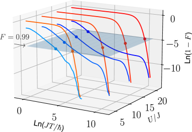
Figure 3: Example case for $N=4$. Infidelity $1-F$ is plotted as a function of the total propagation time $JT/\hbar$ for different values of $U/J$. Here, we define the fidelity $F$ as the closeness of the system state to the NOON state at the end of the driving protocol. The GCD method (blue curves) achieves a NOON state for $U=20J$ with a fidelity $F>0.99$ after $T\approx 100\hbar/J$, whereas the G method (red curves) requires a significantly longer time exceeding $T\approx 3\times 10^{4}\hbar/J$. The plane related to a fidelity of $F=0.99$ is depicted in blue; color dots mark its intersection with infidelities curves.

Results. Figure 3 displays the numerically computed infidelity as a function of the total protocol time $JT/\hbar$ for $N=4$ and different values of $U/J$. This infidelity is defined as $1-F$ with $F=|\langle NOON|\psi(T)\rangle|^{2}$ and $|NOON\rangle=(|N,0,0\rangle+|0,0,N\rangle)/\sqrt{2}$, where $|\psi(t)\rangle$ is the time-dependent state vector of the system starting at $|\psi(0)\rangle=|0,N,0\rangle$. To quantify the impact of counterdiabatic driving, we define by $T_{G}$ and $T_{GCD}$ the protocol time needed to read the fidelity $F=2^{-1/2}=0.71$ with the geodesic protocol (G) and the combined geodesic and counterdiabatic driving (GCD), respectively. For $N=4$ and $U/J=20$, a protocol speed gain factor $g=T_{G}/T_{GCD}=9481$ is calculated. Important gains in the protocol time are also obtained for high fidelities, such as $F=0.99$, as shown in Fig. 3.

Figure 4 shows the time savings factor $T_{G}/T_{GCD}$ for various values of the particle number $N\leq 5$. We clearly see in Fig. 4(a) that the gain increases exponentially with $N$, for various values of interaction $U/J$. More precisely, as is seen in Fig. 4(b), the scaling $T_{G}\sim T_{GCD}(U/J)^{N-1}$ is obtained. This scaling reflects the inverse size of the spectral gap between the two many-body eigenstates that are formed by the $|0,N,0\rangle$ and $|NOON\rangle$ components in the absence of counterdiabatic driving, given by $2\mathcal{J}$ in Eq. (5), which scales as $J(J/U)^{N-1}$ according to perturbation theory (see [38]). As is shown in Fig. 4(c-e), this yields an exponential increase of $T_{G}$ with $N$ at fixed fidelity, which is substantially amended via counterdiabatic driving.

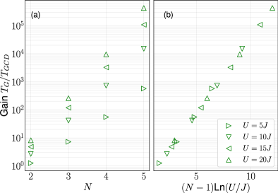
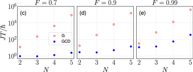
Figure 4: (a),(b) Gain ratio between the times required to achieve a fidelity of $F=0.71$ using the G and GCD methods for various interaction strengths, as a function of the number of particles. We find an exponential increase in efficiency $T_{G}\sim(J/U)^{N-1}$ when using the GCD method compared to the G method. (c),(d),(e) Protocol time $JT/\hbar$ as a function of particle number $N$ needed to yield the fidelity (a) $F=0.7$, (b) $F=0.9$, (c) $F=0.99$ at fixed $NU/J=60$. The exponential increase $T_{G}\sim(J/U)^{N-1}$ is substantially amended by the GCD method.

To better understand these results in terms of a specific physical context, let us consider a gas of ⁸⁷Rb atoms, with $m=1.443\times 10^{-25}$ kg and the s-wave scattering length $a_{s}=5.313$ nm, which is confined in an optical lattice that is generated by lasers with the wavelength $\lambda=1064$ nm, whose lattice site energies are tuned to achieve the adiabatic transition (see [38] for a more detailed description of a possible experimental realization). According to [62, 63, 64, 23], a characteristic hopping time scale in case of the ratio $U/J=20$ is then given by $\hbar/J=4.4\times 10^{-3}$ s. Using this time scale for the example case depicted in Fig. 3, a fidelity of $F=0.98$ is obtained after a duration of 0.264 s with the GCD method. In contrast, using only a geodesic driving will require at least $96.8$ s.

Conclusion. We have demonstrated the feasibility of generating stable NOON states using adiabatic techniques. Specifically, the creation of NOON states can be achieved through the use of the geodesics of the parameter manifold, which is to be complemented by the addition of a counterdiabatic Hamiltonian. This latter key ingredient allows for efficient gap engineering and gives rise to a drastic reduction of the creation time as compared to a purely adiabatic transition protocol, while maintaining its inherent robustness and a highly satisfactory purity of the NOON state.

The realization of NOON states with ultracold atoms in optical lattices thus becomes feasible and is facilitated by the fact that the adaptations of the interaction and hopping parameters that are needed to emulate counterdiabatic driving can be static provided that the adiabatic energy level tuning protocol is preoptimized according to geodesic control. In practice, NOON states can be produced [38] using tunable superlattice techniques [65], synthetic gauge fields for inducing complex hopping [66, 67], quantum gas microscopes for readout [68, 69] possibly to be combined with atom conveyor belts [70, 71], as well as homogeneous lattice techniques to maintain perfect symmetry between the two NOON sites [72]. A combination with chaos-assisted collective tunneling induced by periodic driving [23, 25] and other Floquet engineering techniques [73, 74, 75, 76] appears also possible and opens perspectives towards a realization with $N\sim 10$ particles.

This project (EOS 40007526) has received funding from the FWO and F.R.S.-FNRS under the Excellence of Science (EOS) programme. S. W. thanks A. Smerzi for useful discussions and acknowledges support by Q-DYNAMO (EU HORIZON-MSCA-2022-SE-01) with project No. 101131418 and by the National Recovery and Resilience Plan (PNRR), Mission 4 Component 2 Investment 1.3 – Call for tender No. 341 of 15/03/2022 of Italian MUR funded by NextGenerationEU, with project No. PE0000023, Concession Decree No. 1564 of 11/10/2022 adopted by MUR, CUP D93C22000940001, Project title “National Quantum Science and Technology Institute“ (NQSTI).

Supplemental material

Perturbation theory

We calculate here the terms appearing in the perturbative development for $NU\gg J$. The Hamiltonian of the full system is given by

$$\hat{H}=\frac{U}{2}\sum_{i=1}^{3}\hat{a}_{i}^{\dagger}\hat{a}_{i}^{\dagger}\hat{a}_{i}\hat{a}_{i}-J\hat{a}_{2}^{\dagger}(\hat{a}_{1}+\hat{a}_{3})-J^{*}(\hat{a}_{1}^{\dagger}+\hat{a}_{3}^{\dagger})\hat{a}_{2}$$ (1)

for a complex hopping. Let us denote the interaction energy shifted by the driving term $\varepsilon$ as $E_{n_{1},n_{2},n_{3}}=n_{2}\varepsilon+\sum_{i=1}^{3}Un_{i}(n_{i}-1)/2$ and the hopping terms as $\mathcal{J}_{n_{i},n_{2}}=J\sqrt{n_{i}(n_{2}+1)}$ and $\mathcal{J}_{n_{2},n_{i}}^{*}=J^{*}\sqrt{n_{2}(n_{i}+1)}$, where $n_{i}$ are the number of particles in site $i$. Using the stationary Schrödinger equation, we end up with a system of coupled equations

$$E\Psi_{N,0,0}=E_{N,0,0}\Psi_{N,0,0}-\mathcal{J}_{N\,0}\Psi_{N-1,1,0}$$ (2)

$$E\Psi_{N-1,1,0}=E_{N-1,1,0}\Psi_{N-1,1,0}-\mathcal{J}_{1,N-1}^{*}\Psi_{N,0,0}$$ (3)

$$-\mathcal{J}_{N-1,1}\Psi_{N-2,2,0}-\mathcal{J}_{1,0}^{*}\Psi_{N-1,0,1}$$

$$E\Psi_{N-2,2,0}=E_{N-2,2,0}\Psi_{N-2,2,0}-\mathcal{J}_{2,N-2}^{*}\Psi_{N-1,1,0}$$ (4)

$$-\mathcal{J}_{N-2,2}\Psi_{N-3,3,0}-\mathcal{J}_{2,0}^{*}\Psi_{N-2,1,1}$$

$$E\Psi_{N-1,0,1}=E_{N-1,0,1}\Psi_{N-1,0,1}-\mathcal{J}_{1,0}\Psi_{N-1,1,0}$$ (5)

$$-\mathcal{J}_{N-1,0}\Psi_{N-2,1,1}$$

$$...$$ (6)

$$E\Psi_{0,0,N}=E_{0,0,N}\Psi_{0,0,N}-\mathcal{J}_{N,0}\Psi_{0,1,N-1}$$ (7)

This set of equations can be mapped to a set of paths that the system can take to travel through the Hilbert space from $|N,0,0\rangle$ to $|0,0,N\rangle$, as depicted in Fig. 1.

For our study, we limit ourselves to the fourth order. For this purpose, we calculate the contributions of the following paths:

$$|N,0,0\rangle\leftrightarrow|N-1,1,0\rangle\leftrightarrow|N-2,2,0\rangle$$

$$|N,0,0\rangle\leftrightarrow|N-1,1,0\rangle\leftrightarrow|N-1,0,1\rangle$$

$$|N,0,0\rangle\leftrightarrow|N-1,1,0\rangle\leftrightarrow|N,0,0\rangle$$

which will add a perturbative correction $\mathcal{E}(U,J)$ to the interaction energy of the state $|N,0,0\rangle$ :

$$E\Psi_{N,0,0}=(E_{N,0,0}+\mathcal{E}(U,J))\Psi_{N,0,0}$$ (8)

By solving for the considered trajectories, we obtain

$$\mathcal{E}(U,J)=\frac{\mathcal{J}_{N\to 0}^{2}}{E^{(2)}-\frac{\mathcal{J}_{N-1,1,0}^{2}}{E-E_{N-2,2,0}}-\frac{\mathcal{J}_{1\to 0}^{2}}{E-E_{N-1,0,1}}}$$ (9)

where $E^{(2)}=E_{N,0,0}-E_{N-1,1,0}+\mathcal{J}_{N\to 0}^{2}/(E_{N,0,0}-E_{N-1,1,0})$. Expanding for $E\gg\mathcal{J}$, the corrective term is

$$\mathcal{E}(U,J)=\frac{NJ^{2}}{(N-1)U}+\frac{NJ^{4}}{(N-1)^{2}(N-2)U^{3}}$$ (10)

Figure 1: Schematic diagram of the various trajectories the system can take within the Hilbert space for $N=4$ particles. The vertical axis is the total interaction energy. The most probable path, i.e., the one contributing the most to the perturbative terms, is depicted in bold.

Since the central state $|0,N,0\rangle$ is symmetrically coupled to the other two states, the value of $\tilde{\mathcal{E}}(U,J)$ at the second order will be twice the value of $\mathcal{E}(U,J)$, but a correction appears at the fourth order. Computing this new contribution leads to identify

$$\tilde{\mathcal{E}}(U,J)=2\mathcal{E}(U,J)-\frac{2N|J|^{4}}{(N-1)^{2}(N-2)U^{3}}$$ (11)

$$\times\left[\frac{N^{2}-6N+7}{(N-1)(2N-3)}+1\right]$$

At this point, we are still neglecting the bias $\varepsilon$ induced by the modified energies. The full Hamiltonian is therefore $H+\varepsilon\hat{a}_{2}^{\dagger}\hat{a}_{2}$. Indeed, $\varepsilon$ depends on time since the energy of the central well is driven according to the protocol. Consequently, the instantaneous eigenenergies of the $N$-particle system are also time-dependent. Applying a suitable gauge transformation allows us to absorb the time dependence into the central well. We then have the energies, incorporating corrective terms and the driving:

$$\tilde{\Sigma}(U,J,\varepsilon)=UN(N-1)/2+\tilde{\mathcal{E}}(U,J)$$ (12)

$$+\frac{N|J|^{2}}{(N-1)U}\varepsilon+\mathcal{N}\varepsilon$$

$$\Sigma(U,J,\varepsilon)=UN(N-1)/2+\mathcal{E}(U,J)$$ (13)

$$+\frac{N|J|^{2}}{(N-1)U}\varepsilon$$

We thus obtain the following expression for the shifted number of particles:

$$\mathcal{N}=N+\delta N=N[1-3|J|^{2}/((N-1)U)^{2}].$$ (14)

The effective coupling term between $|N,0,0\rangle$ and $|0,N,0\rangle$ is calculated from the trajectory depicted in bold in Fig. 1. By symmetry, the coupling must be the same between $|0,N,0\rangle$ and $|0,0,N\rangle$. We obtain

$$\mathcal{J}(U,J)=-\frac{NJ^{N}}{(N-1)!U^{N-1}}$$ (15)

With those parameters, one can fully determine the reduced Hamiltonian $H_{\text{red}}$.

Specific proposal for a realization of a NOON state lattice

In this section, we outline a specific quantitative proposal how to realize a periodic lattice of NOON states with bosonic atoms.

We consider for this purpose a gas of ultracold bosonic atoms that is prepared within a three-dimensional optical square lattice. The system is supposed to be in the Mott insulator regime, where inter-site hopping is totally suppressed along two of the three lattice axes and also rather weak compared to on-site atom-atom interaction for the remaining third axis. Along this third axis, a superlattice configuration involving three periods is to be implemented, quantitatively described, e.g., by the effective potential

$$V(x)=V_{0}\left[0.5\cos(kx)-2\cos(2kx)+\eta(t)\cos(kx/2)\right]$$ (16)

where $V_{0}$ is a suitable lattice height scale, $k$ is the characteristic lattice wave number, and $\eta(t)$ describes the dimensionless amplitude of the lattice component with the largest period $4\pi/k$. Tuning $\eta$ as a function of time in a precisely controlled manner allows one then to induce the adiabatic transition through which NOON states can be created.

The initial superlattice configuration ought to be such that pronounced minima appear on every fourth lattice site. As can be seen in Fig. 2(a), this can be achieved e.g. by the choice $\eta=-4$ for the control amplitude. This lattice is to be loaded with a gas of ultracold bosonic atoms, such that one has a mean population of $N/4$ atoms per lattice site where $N$ is the particle number for which the NOON state is to be created. Subsequent cooling this gas to ultralow temperatures gives then rise to a Mott insulator state where every fourth site of the superlattice is populated by $N$ atoms.

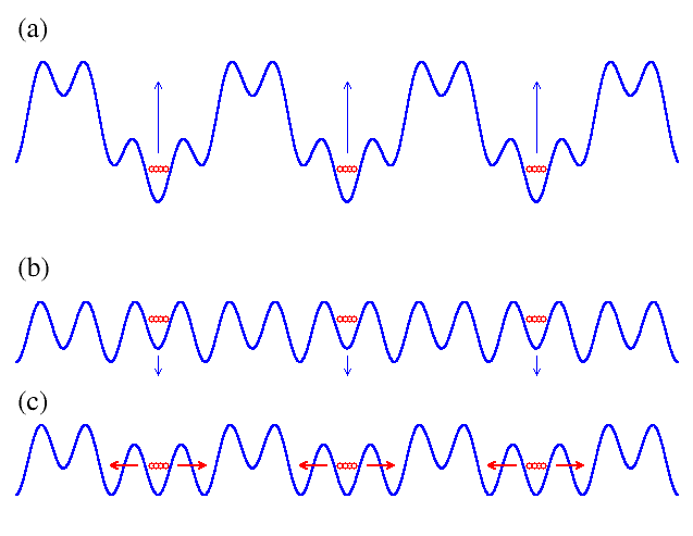
Figure 2: Schematic representation of the protocol to be implemented for the creation of the NOON state. (a) The starting configuration is a superlattice with four characteristic wave numbers, featuring a distinct ground well within each superlattice cell. These ground wells are then populated with $N$ atoms per well. (b) At time $t=0$ one of the superlattice amplitudes is suddenly increased such that the former ground wells now lie energetically above their two neighbor wells. The counterdiabatic driving protocol can then be started. (c) At resonance with the neighboring wells the adiabatic transition takes place giving rise to the NOON state superposition. The blue lines in the panels represent the potential (16) for the parameter (a) $\eta=-4$, (b) $\eta=0$, and (c) $\eta=-1$.

At time $t=0$, a quench is to be implemented by which means the on-site energies of the populated lattice sites becomes suddenly increased, thus slightly exceeding the energies on the adjacent sites. As illustrated in Fig. 2(b), this can be achieved by suddenly increasing the amplitude $\eta$ from $-4$ to $0$. The resulting (two-period) superlattice configuration can be considered to be the starting point for the NOON state creation process to be implemented. The amplitude $\eta$ has then to be slowly decreased, according to the protocol that we discuss in the main text of the paper. In addition, an artificial gauge field has to be induced along the lattice [1, 2] in order to give rise to the complex hopping matrix element (see Eq. 10 of the manuscript) that is required for the implementation of the counterdiabatic driving protocol. Additional (even time-dependent) adaptations of the Bose-Hubbard parameters can, if needed, be achieved by suitable variations of the global lattice amplitude $V_{0}$ as well as of the analogous amplitudes along the other two axes of the lattice.

As discussed in the main part of the paper, the NOON states are then produced as soon as the populated sites of the lattice have approximately the same energy as their two neighbor sites. As illustrated in Fig. 2(c), this is roughly the case for $\eta=-1$. Further tuning the initially populated (and now depopulated) sites to lower energies then gives rise to a NOON state lattice in which every second site may or may not host $N$ atoms. This can then be verified by quantum gas microscopes [3, 4]. A suitable atom transport protocol [5, 6] can then be used to direct the two components $|N,0\rangle$ and $|0,N\rangle$ of each NOON pair into spatially separate directions, for possible usage in the context of quantum metrological applications.

Note that next-to-nearest neighbor hoppings of atoms, while technically possible, can be safely neglected since they take place on time scales that are much larger than the (already very large) time scales for the creation of the NOON state. The maintaining of nearly perfect homogeneity along the lattice, which is a key requirement for this protocol to work out correctly, is certainly a great challenge but can be, in principle, achieved using flat lattice potentials [7].

References

- Einstein et al. [1935] A. Einstein, B. Podolsky, and N. Rosen, Can Quantum-Mechanical Description of Physical Reality Be Considered Complete?, Phys. Rev. 47, 777 (1935).
- Nielsen and Chuang [2010] M. A. Nielsen and I. L. Chuang, Quantum Computation and Quantum Information: 10th Anniversary Edition (Cambridge University Press, 2010).
- Degen et al. [2017] C. L. Degen, F. Reinhard, and P. Cappellaro, Quantum sensing, Rev. Mod. Phys. 89, 035002 (2017).
- Pezzè et al. [2018] L. Pezzè, A. Smerzi, M. K. Oberthaler, R. Schmied, and P. Treutlein, Quantum metrology with nonclassical states of atomic ensembles, Rev. Mod. Phys. 90, 035005 (2018).
- Kwon et al. [2019] H. Kwon, K. C. Tan, T. Volkoff, and H. Jeong, Nonclassicality as a Quantifiable Resource for Quantum Metrology, Phys. Rev. Lett. 122, 040503 (2019).
- Pezzè and Smerzi [2020] L. Pezzè and A. Smerzi, Heisenberg-Limited Noisy Atomic Clock Using a Hybrid Coherent and Squeezed State Protocol, Phys. Rev. Lett. 125, 210503 (2020).
- Ye and Zoller [2024] J. Ye and P. Zoller, Essay: Quantum Sensing with Atomic, Molecular, and Optical Platforms for Fundamental Physics, Phys. Rev. Lett. 132, 190001 (2024).
- Afek et al. [2010] I. Afek, O. Ambar, and Y. Silberberg, High-NOON States by Mixing Quantum and Classical Light, Science 328, 879 (2010).
- Song et al. [2017] C. Song, K. Xu, W. Liu, C.-P. Yang, S.-B. Zheng, H. Deng, Q. Xie, K. Huang, Q. Guo, L. Zhang, P. Zhang, D. Xu, D. Zheng, X. Zhu, H. Wang, Y.-A. Chen, C.-Y. Lu, S. Han, and J.-W. Pan, 10-Qubit Entanglement and Parallel Logic Operations with a Superconducting Circuit, Phys. Rev. Lett. 119, 180511 (2017).
- Zhang et al. [2018] J. Zhang, M. Um, D. Lv, J.-N. Zhang, L.-M. Duan, and K. Kim, NOON States of Nine Quantized Vibrations in Two Radial Modes of a Trapped Ion, Phys. Rev. Lett. 121, 160502 (2018).
- Cirac et al. [1998] J. I. Cirac, M. Lewenstein, K. Mølmer, and P. Zoller, Quantum superposition states of Bose-Einstein condensates, Phys. Rev. A 57, 1208 (1998).
- Gordon and Savage [1999] D. Gordon and C. M. Savage, Creating macroscopic quantum superpositions with Bose-Einstein condensates, Phys. Rev. A 59, 4623 (1999).
- Sørensen et al. [2001] A. Sørensen, L.-M. Duan, J. I. Cirac, and P. Zoller, Many-particle entanglement with Bose–Einstein condensates, Nature 409, 63–66 (2001).
- Micheli et al. [2003] A. Micheli, D. Jaksch, J. I. Cirac, and P. Zoller, Many-particle entanglement in two-component Bose-Einstein condensates, Phys. Rev. A 67, 013607 (2003).
- Mahmud et al. [2003] K. W. Mahmud, H. Perry, and W. P. Reinhardt, Phase engineering of controlled entangled number states in a single component Bose–Einstein condensate in a double well, J. Phys. B: At. Mol. Opt. Phys 36, L265 (2003).
- Teichmann and Weiss [2007] N. Teichmann and C. Weiss, Coherently controlled entanglement generation in a binary Bose-Einstein condensate, EPL 78, 10009 (2007).
- Schneider Grün et al. [2022] D. Schneider Grün, K. Wittmann Wilsmann, L. Ymai, J. Links, and A. Foerster, Protocol designs for NOON states, Commun Phys 5 (2022).
- Milburn et al. [1997] G. J. Milburn, J. Corney, E. M. Wright, and D. F. Walls, Quantum dynamics of an atomic Bose-Einstein condensate in a double-well potential, Phys. Rev. A 55, 4318 (1997).
- Smerzi et al. [1997] A. Smerzi, S. Fantoni, S. Giovanazzi, and S. R. Shenoy, Quantum Coherent Atomic Tunneling between Two Trapped Bose-Einstein Condensates, Phys. Rev. Lett. 79, 4950 (1997).
- Strzys et al. [2008] M. P. Strzys, E. M. Graefe, and H. J. Korsch, Kicked Bose–Hubbard systems and kicked tops—destruction and stimulation of tunneling, New J. Phys. 10, 013024 (2008).
- Carr et al. [2010] L. D. Carr, D. R. Dounas-Frazer, and M. A. Garcia-March, Dynamical realization of macroscopic superposition states of cold bosons in a tilted double well, EPL 90, 10005 (2010).
- Salgueiro et al. [2007] A. N. Salgueiro, A. de Toledo Piza, G. B. Lemos, R. Drumond, M. C. Nemes, and M. Weidemüller, Quantum dynamics of bosons in a double-well potential: Josephson oscillations, self-trapping and ultralong tunneling times, Eur. Phys. J. D 44, 537 (2007).
- Vanhaele and Schlagheck [2021] G. Vanhaele and P. Schlagheck, NOON states with ultracold bosonic atoms via resonance- and chaos-assisted tunneling, Phys. Rev. A 103, 013315 (2021).
- Tomsovic and Ullmo [1994] S. Tomsovic and D. Ullmo, Chaos-assisted tunneling, Phys. Rev. E 50, 145 (1994).
- Vanhaele et al. [2022] G. Vanhaele, A. Bäcker, R. Ketzmerick, and P. Schlagheck, Creating triple-NOON states with ultracold atoms via chaos-assisted tunneling, Phys. Rev. A 106, L011301 (2022).
- Chen et al. [2010] X. Chen, A. Ruschhaupt, S. Schmidt, A. del Campo, D. Guéry-Odelin, and J. G. Muga, Fast Optimal Frictionless Atom Cooling in Harmonic Traps: Shortcut to Adiabaticity, Phys. Rev. Lett. 104, 063002 (2010).
- del Campo [2013] A. del Campo, Shortcuts to Adiabaticity by Counterdiabatic Driving, Phys. Rev. Lett. 111, 100502 (2013).
- Deffner et al. [2014] S. Deffner, C. Jarzynski, and A. del Campo, Classical and quantum shortcuts to adiabaticity for scale-invariant driving, Phys. Rev. X 4, 021013 (2014).
- Guéry-Odelin et al. [2019] D. Guéry-Odelin, A. Ruschhaupt, A. Kiely, E. Torrontegui, S. Martínez-Garaot, and J. G. Muga, Shortcuts to adiabaticity: Concepts, methods, and applications, Rev. Mod. Phys. 91, 045001 (2019).
- del Campo and Kim [2019] A. del Campo and K. Kim, Focus on shortcuts to adiabaticity, New J. Phys. 21, 050201 (2019).
- Čepaitė et al. [2023] I. Čepaitė, A. Polkovnikov, A. J. Daley, and C. W. Duncan, Counterdiabatic Optimized Local Driving, PRX Quantum 4, 010312 (2023).
- Demirplak and Rice [2003] M. Demirplak and S. Rice, Adiabatic Population Transfer with Control Fields, J. Phys. Chem. A 107 (2003).
- Demirplak and Rice [2008] M. Demirplak and S. A. Rice, On the consistency, extremal, and global properties of counterdiabatic fields, J. Chem. Phys. 129, 154111 (2008).
- Kolodrubetz et al. [2013] M. Kolodrubetz, V. Gritsev, and A. Polkovnikov, Classifying and measuring geometry of a quantum ground state manifold, Phys. Rev. B 88, 064304 (2013).
- Tomka et al. [2016] M. Tomka, T. Souza, S. Rosenberg, and A. Polkovnikov, Geodesic Paths for Quantum Many-Body Systems, (2016), arXiv:1606.05890 .
- Fisher et al. [1989] M. P. A. Fisher, P. B. Weichman, G. Grinstein, and D. S. Fisher, Boson localization and the superfluid-insulator transition, Phys. Rev. B 40, 546 (1989).
- Greiner et al. [2002] M. Greiner, O. Mandel, T. Esslinger, T. W. Hänsch, and I. Bloch, Quantum phase transition from a superfluid to a Mott insulator in a gas of ultracold atoms, Nature 415, 39 (2002).
- [38] See Supplemental Material.
- Born and Fock [1928] M. Born and V. Fock, Beweis des Adiabatensatzes, Zeitschrift für Physik 51, 165 (1928).
- Landau [1932] L. Landau, Zur theorie der energieubertragung. ii, Physikalische Zeitschrift der Sowjetunion 2, 46 (1932).
- Zener [1932] C. Zener, Non-adiabatic crossing of energy levels, Proc. R. Soc. Lond. A 137, 696 (1932).
- Stückelberg [1932] E. Stückelberg, Theorie der unelastischen Stösse zwischen Atomen, Helv. Phys. Acta 5, 369 (1932).
- Majorana [1932] E. Majorana, Atomi orientati in campo magnetico variabile, Il Nuovo Cimento (1924-1942) 9, 43 (1932).
- Berry [1987] M. V. Berry, Quantum Phase Corrections from Adiabatic Iteration, Proc. R. Soc. Lond. A 414, 31 (1987).
- Unanyan et al. [1997] R. Unanyan, L. Yatsenko, K. Bergmann, and B. Shore, Laser-induced adiabatic atomic reorientation with control of diabatic losses, Optics Communications 139, 48 (1997).
- Fleischhauer et al. [1999] M. Fleischhauer, R. Unanyan, B. W. Shore, and K. Bergmann, Coherent population transfer beyond the adiabatic limit: Generalized matched pulses and higher-order trapping states, Phys. Rev. A 59, 3751 (1999).
- Lim and Berry [1991] R. Lim and M. V. Berry, Superadiabatic tracking of quantum evolution, J. Phys. A: Math. Gen. 24, 3255 (1991).
- Provost and Vallee [1980] J. P. Provost and G. Vallee, Riemannian structure on manifolds of quantum states, Commun.Math. Phys. 76, 289 (1980).
- Kolodrubetz et al. [2017] M. Kolodrubetz, D. Sels, P. Mehta, and A. Polkovnikov, Geometry and non-adiabatic response in quantum and classical systems, Physics Reports 697, 1 (2017).
- Berry [2009] M. V. Berry, Transitionless quantum driving, J. Phys. A: Math. Theor. 42, 365303 (2009).
- Bason et al. [2012] M. G. Bason, M. Viteau, N. Malossi, P. Huillery, E. Arimondo, D. Ciampini, R. Fazio, V. Giovannetti, R. Mannella, and O. Morsch, High-fidelity quantum driving, Nature Physics 8, 147 (2012).
- Sels and Polkovnikov [2017] D. Sels and A. Polkovnikov, Minimizing irreversible losses in quantum systems by local counterdiabatic driving, PNAS 114, E3909 (2017).
- Claeys et al. [2019] P. W. Claeys, M. Pandey, D. Sels, and A. Polkovnikov, Floquet-Engineering Counterdiabatic Protocols in Quantum Many-Body Systems, Phys. Rev. Lett. 123, 090602 (2019).
- Mbeng and Lechner [2022] G. B. Mbeng and W. Lechner, Rotated ansatz for approximate counterdiabatic driving, (2022), arXiv:2207.03553 .
- Prielinger et al. [2021] L. Prielinger, A. Hartmann, Y. Yamashiro, K. Nishimura, W. Lechner, and H. Nishimori, Two-parameter counter-diabatic driving in quantum annealing, Phys. Rev. Res. 3, 013227 (2021).
- Petiziol et al. [2024] F. Petiziol, F. Mintert, and S. Wimberger, Quantum control by effective counterdiabatic driving, EPL 145, 15001 (2024).
- Yagüe Bosch et al. [2023] L. S. Yagüe Bosch, T. Ehret, F. Petiziol, E. Arimondo, and S. Wimberger, Shortcut-to-Adiabatic Controlled-Phase Gate in Rydberg Atoms, Annalen der Physik 535, 2300275 (2023).
- Takahashi and del Campo [2024] K. Takahashi and A. del Campo, Shortcuts to Adiabaticity in Krylov Space, Phys. Rev. X 14, 011032 (2024).
- Eckardt et al. [2005] A. Eckardt, C. Weiss, and M. Holthaus, Superfluid-Insulator Transition in a Periodically Driven Optical Lattice, Phys. Rev. Lett. 95, 260404 (2005).
- Creffield and Monteiro [2006] C. E. Creffield and T. S. Monteiro, Tuning the Mott Transition in a Bose-Einstein Condensate by Multiple Photon Absorption, Phys. Rev. Lett. 96, 210403 (2006).
- Lignier et al. [2007] H. Lignier, C. Sias, D. Ciampini, Y. Singh, A. Zenesini, O. Morsch, and E. Arimondo, Dynamical Control of Matter-Wave Tunneling in Periodic Potentials, Phys. Rev. Lett. 99, 220403 (2007).
- Garg [2000] A. Garg, Tunnel splittings for one-dimensional potential wells revisited, Am. J. Phys. 68, 430–437 (2000).
- Foot [2005] C. Foot, Atomic Physics, Oxford Master Series in Physics (OUP Oxford, 2005).
- Michon et al. [2018] E. Michon, C. Cabrera-Gutiérrez, A. Fortun, M. Berger, M. Arnal, V. Brunaud, J. Billy, C. Petitjean, P. Schlagheck, and D. Guéry-Odelin, Phase transition kinetics for a Bose Einstein condensate in a periodically driven band system, New J. Phys. 20, 053035 (2018).
- Fölling et al. [2007] S. Fölling, S. Trotzky, P. Cheinet, M. Feld, R. Saers, A. Widera, T. Müller, and I. Bloch, Direct observation of second-order atom tunnelling, Nature 448, 1029–1032 (2007).
- Galitski et al. [2019] V. Galitski, G. Juzeliūnas, and I. B. Spielman, Artificial gauge fields with ultracold atoms, Physics Today 72, 38 (2019).
- Dalibard et al. [2011] J. Dalibard, F. Gerbier, G. Juzeliūnas, and P. Öhberg, Colloquium: Artificial gauge potentials for neutral atoms, Rev. Mod. Phys. 83, 1523 (2011).
- Bakr et al. [2009] W. S. Bakr, J. I. Gillen, A. Peng, S. Fölling, and M. Greiner, A quantum gas microscope for detecting single atoms in a Hubbard-regime optical lattice, Nature 462, 74 (2009).
- Sherson et al. [2010] J. F. Sherson, C. Weitenberg, M. Endres, M. Cheneau, I. Bloch, and S. Kuhr, Single-atom-resolved fluorescence imaging of an atomic Mott insulator, Nature 467, 68 (2010).
- Kuhr et al. [2003] S. Kuhr, W. Alt, D. Schrader, I. Dotsenko, Y. Miroshnychenko, W. Rosenfeld, M. Khudaverdyan, V. Gomer, A. Rauschenbeutel, and D. Meschede, Coherence Properties and Quantum State Transportation in an Optical Conveyor Belt, Phys. Rev. Lett. 91, 213002 (2003).
- Browaeys et al. [2005] A. Browaeys, H. Häffner, C. McKenzie, S. L. Rolston, K. Helmerson, and W. D. Phillips, Transport of atoms in a quantum conveyor belt, Phys. Rev. A 72, 053605 (2005).
- Gaunt et al. [2013] A. L. Gaunt, T. F. Schmidutz, I. Gotlibovych, R. P. Smith, and Z. Hadzibabic, Bose-Einstein Condensation of Atoms in a Uniform Potential, Phys. Rev. Lett. 110, 200406 (2013).
- Goldman and Dalibard [2014] N. Goldman and J. Dalibard, Periodically Driven Quantum Systems: Effective Hamiltonians and Engineered Gauge Fields, Phys. Rev. X 4, 031027 (2014).
- Bukov et al. [2015] M. Bukov, L. D’Alessio, and A. Polkovnikov, Universal high-frequency behavior of periodically driven systems: from dynamical stabilization to Floquet engineering, Advances in Physics 64, 139 (2015).
- Eckardt [2017] A. Eckardt, Colloquium: Atomic quantum gases in periodically driven optical lattices, Rev. Mod. Phys. 89, 011004 (2017).
- Weitenberg and Simonet [2021] C. Weitenberg and J. Simonet, Tailoring quantum gases by Floquet engineering, Nature Physics 17, 1342 (2021).

References

- Dalibard et al. [2011] J. Dalibard, F. Gerbier, G. Juzeliūnas, and P. Öhberg, Colloquium: Artificial gauge potentials for neutral atoms, Rev. Mod. Phys. 83, 1523 (2011).
- Galitski et al. [2019] V. Galitski, G. Juzeliūnas, and I. B. Spielman, Artificial gauge fields with ultracold atoms, Physics Today 72, 38 (2019).
- Bakr et al. [2009] W. S. Bakr, J. I. Gillen, A. Peng, S. Fölling, and M. Greiner, A quantum gas microscope for detecting single atoms in a Hubbard-regime optical lattice, Nature 462, 74 (2009).
- Sherson et al. [2010] J. F. Sherson, C. Weitenberg, M. Endres, M. Cheneau, I. Bloch, and S. Kuhr, Single-atom-resolved fluorescence imaging of an atomic Mott insulator, Nature 467, 68 (2010).
- Kuhr et al. [2003] S. Kuhr, W. Alt, D. Schrader, I. Dotsenko, Y. Miroshnychenko, W. Rosenfeld, M. Khudaverdyan, V. Gomer, A. Rauschenbeutel, and D. Meschede, Coherence Properties and Quantum State Transportation in an Optical Conveyor Belt, Phys. Rev. Lett. 91, 213002 (2003).
- Browaeys et al. [2005] A. Browaeys, H. Häffner, C. McKenzie, S. L. Rolston, K. Helmerson, and W. D. Phillips, Transport of atoms in a quantum conveyor belt, Phys. Rev. A 72, 053605 (2005).
- Gaunt et al. [2013] A. L. Gaunt, T. F. Schmidutz, I. Gotlibovych, R. P. Smith, and Z. Hadzibabic, Bose-Einstein Condensation of Atoms in a Uniform Potential, Phys. Rev. Lett. 110, 200406 (2013).