The SUPER excitation of quantum emitters is a multi-photon process

The swing-up of quantum emitter population (SUPER) scheme allows to populate the excited state of a quantum emitter with near-unity fidelity using two red-detuned laser pulses. Its off-resonant, yet fully coherent nature has attracted significant interest in quantum photonics as a valuable tool for preparing single-photon sources in their excited state on demand, while simultaneously ensuring straightforward spectral filtering of the laser. However, the physical understanding of this mechanism in terms of energy exchange between the electromagnetic field and the emitter is still lacking. Here, we present a fully quantized model of the swing-up excitation and demonstrate that it is in fact a multi-photon process, where one of the modes loses two or more photons while the other gains at least one. Our findings provide an unexpected physical interpretation of the SUPER scheme and unveil a new non-linear interaction between single emitters and multiple field modes.

1 Introduction

Efficient sources of indistinguishable single photons are essential components of optical quantum computers and simulators [1, 2]. Whereas spontaneous parameteric downconversion allows for straightforward generation of highly indistinguishable heralded photons, its probabilistic nature leads to low single-photon purity and collection efficiency, which can only be improved with complex multiplexing schemes [3, 4]. On the other hand, quantum emitters based on semiconductor quantum dots yield nowadays highly indistinguishable single photons with high purity and collection efficiency of the order of $\approx 0.6$ [5, 6, 2]. Activating such sources on demand calls for a fast and coherent optical excitation protocol that prepares the emitter in the desired excited state.

In the so-called swing-up of quantum emitter population (SUPER) scheme [7], two red-detuned laser pulses interacting simultaneously with the emitter cause fast oscillations of the excited state population. For a proper choice of the laser parameters (frequency, amplitude, and duration of each pulse), the emitter is finally left in the excited state with fidelity close to 100%. The technological advantage of this technique, as compared for example with resonant fluorescence, is that laser rejection is straightforwardly achieved via spectral filtering due to the red-detuned nature of the pump [8, 9]. Moreover, it populates the excited state directly with a fast and coherent process, as opposed for example to pumping into higher energy levels (which requires incoherent internal relaxation to create the exciton). This attractive scenario had stimulated intense theoretical and experimental research, including the prospect of applying this technique to cavity-coupled quantum dots [10, 11], the analysis of the important role played by phonon scattering [12, 13, 14], and the possibility of achieving a similar effect with hybrid acousto-optical methods [15]. While the SUPER scheme was originally devised for semiconductor quantum dots, it relies in fact on general properties of quantum emitters coupled to the electromagnetic field and has now been investigated in different material platforms, such as tin vacancies in diamond [16] and emitters in the layered transition metal dichalcogenide WSe₂ [13].

In spite of this active interest, the physical origin of this effect is not yet fully understood. Bracht et al. [17] have explained the swing-up effect with a dressed state picture of the emitter-field system. While one of the laser pulses is dressing the bare emitter states and effectively modify their energy splitting, the other one drives transition between the dressed states. However, a fundamental interpretation in terms of energy exchange between the emitter and the electromagnetic field is still missing. For example, whereas resonance fluorescence is easily interpreted in terms of absorption of one single photon from the laser pump, such a simple picture is currently unavailable for the SUPER scheme. This is further complicated by the off-resonant nature of this protocol and by the presence of two simultaneous laser fields, which makes the physical interpretation less intuitive.

In this work, we surprisingly show that the SUPER scheme excitation involves multiple photon exchanges between the emitter and the laser. We achieve this by developing a quantum-mechanical model for an emitter coupled to two quantized field modes, which allows to count the number of photons in each mode before and after interaction with the emitter. Specifically, we find that two photons are typically absorbed from one of the modes during the swing-up process. Of these two excitations, one is stored in the emitter by raising its population from the ground to the excited state, while the remaining one is absorbed into the second field mode. Interestingly, we find that population inversion may still occur even when one of the field modes is in the vacuum state, provided that the other one is populated with at least two photons.

This article is organized as follows. First, we describe the model and the methodology in Section 2. Adopting a Fock state assumption for the electromagnetic field, we analyze the dynamics of the SUPER and the red-and-blue dichromatic scheme [18, 12] in the large photon number regime in Sections 3 and 4, respectively. We then focus on the few-photon regime in Section 5, where we consider the case where one of the field modes is in the vacuum state. In Section 6, we describe the field in terms of coherent states, and compare the results with the ones obtained under a Fock state assumption. We finally discuss our findings in Section 7, before drawing our conclusions in Section 8.

2 Model

We model the quantum emitter as a two-level system with ground state $\ket{G}$ and excited state $\ket{X}$. Its Hamiltonian is $H_{0}=\hbar\omega_{0}\sigma^{\dagger}\sigma$, with $\sigma^{\dagger}=\outerproduct{X}{G}$ the raising operator. The emitter is coupled to two quantized electromagnetic field modes with Hamiltonian $H_{j}=\hbar\omega_{j}a^{\dagger}_{j}a_{j}$, $j\in\quantity{1,2}$, where $a_{j}$ is the annihilation operator for mode $j$. Using the rotating wave approximation, the emitter-field coupling is modeled as a two-mode Jaynes-Cummings Hamiltonian,

$$H_{\rm int}(t)=\sum_{j=1,2}\hbar g_{j}\exp\quantity(-\frac{t^{2}}{t_{p}^{2}})\quantity(\sigma^{\dagger}a_{j}+\sigma a_{j}^{\dagger}).$$ (1)

The coupling constants $g_{j}$ in Eq. (1) are modulated by a time-dependent Gaussian envelope $\exp\quantity(-\frac{t^{2}}{t_{p}^{2}})$ to simulate pulsed excitation.

In the single-mode Jaynes-Cummings model, the excitation number $\mathcal{N}=\sigma^{\dagger}\sigma+a^{\dagger}a$ is a conserved quantity. It follows that the subspace spanned by the pair $\quantity{\ket{X,n},\ket{G,n+1}}$, satisfying $\expectationvalue{\mathcal{N}}=n+1$, is decoupled from the rest of the Hilbert space. This makes it possible to solve the problem analytically, even in the presence of time-dependent coupling [19, 20, 21]. Similarly, the two-mode Jaynes-Cummings model has a conserved excitation number $\mathcal{N}=\sigma^{\dagger}\sigma+a_{1}^{\dagger}a_{1}+a_{2}^{\dagger}a_{2}$. However, in contrast with the single-mode model, the subspace with constant excitation number $\expectationvalue{\mathcal{N}}=n+1$ is spanned by the set of states $\quantity{\ket{G,n+1,0},\ket{X,n,0},\ket{G,n,1},\ket{X,n-1,1},\ldots,\ket{G,0,n+1}}$ and has dimension $2(n+1)+1$, thereby making the analytical solution challenging.

We thus calculate the dynamics numerically by solving the Schrodinger equation $i\hbar\partial_{t}\ket{\psi(t)}=\widehat{H}_{\rm int}(t)\ket{\psi(t)}$ in the interaction picture with respect to $H_{0}+H_{1}+H_{2}$, with

$$\widehat{H}_{\rm int}(t) =\exp\quantity[\frac{i}{\hbar}(H_{0}+H_{1}+H_{2})t]H_{\rm int}(t)\exp\quantity[-\frac{i}{\hbar}(H_{0}+H_{1}+H_{2})t]$$

$$=\sum_{j=1,2}\hbar g_{j}\exp\quantity(-\frac{t^{2}}{t_{p}^{2}})\quantity(e^{-i\delta_{j}t}\sigma^{\dagger}a_{j}+e^{+i\delta_{j}t}\sigma a_{j}^{\dagger}),$$ (2)

and $\delta_{j}=\omega_{j}-\omega_{0}$ the detuning of each mode with respect to the emitter frequency. Specifically, noting that $\exp\quantity(-3^{2})\approx 10^{-4}$, we initialize the system in the chosen initial state $\ket{\psi(t_{\rm i})}$ at time $t_{\rm i}=-3t_{p}$ and we calculate the evolution of $\ket{\psi(t)}$ with a 4th order Runge-Kutta algorithm until the final state $\ket{\psi(t_{\rm f})}$ at time $t_{\rm f}=+3t_{p}$, where the population of the emitter and each field mode is inspected. Here, the use of the interaction picture is beneficial to avoid fast oscillating terms, especially when dealing with field states with a large number of photons.

It is worth noticing that the numerical algorithm does not preserve the state normalization. This is easily verified with a 1st order Euler method by noticing that the evolved state $\ket{\psi(t+\differential{t})}=\ket{\psi(t)}-\frac{i}{\hbar}\differential{t}\widehat{H}_{\rm int}\ket{\psi(t)}$ satisfies $\innerproduct{\psi(t+\differential{t})}{\psi(t+\differential{t})}=\innerproduct{\psi(t)}{\psi(t)}+\frac{(\differential t)^{2}}{\hbar^{2}}\innerproduct{\widehat{H}_{\rm int}\psi(t)}{\widehat{H}_{\rm int}\psi(t)}>1$, even for $\innerproduct{\psi(t)}{\psi(t)}=1$. Therefore, we take care of normalizing the quantum state to 1 after each step in the calculation.

For the numerical implementation, the state of each field mode $j$ is expanded on a truncated number state basis $\quantity{\ket{n_{j}}}$, with $n_{j}\in(N_{j}^{\rm min},\ldots,N_{j}^{\rm max})$, and operators acting on mode $j$ are represented as $M_{j}\times M_{j}$ matrices, with $M_{j}=N_{j}^{\rm max}-N_{j}^{\rm min}+1$. We make sure that results are converged with respect to the choice of $N_{j}^{\rm max}$ and $N_{j}^{\rm min}$. This can be checked, for instance, by ensuring that the expectation value of the excitation number $\mathcal{N}=\sigma^{\dagger}\sigma+a_{1}^{\dagger}a_{1}+a_{2}^{\dagger}a_{2}$ is conserved throughout the simulation, as required by the fact that $\commutator{\widehat{H}_{\rm int}(t)}{\mathcal{N}}=0$.

3 Dynamics of the SUPER scheme

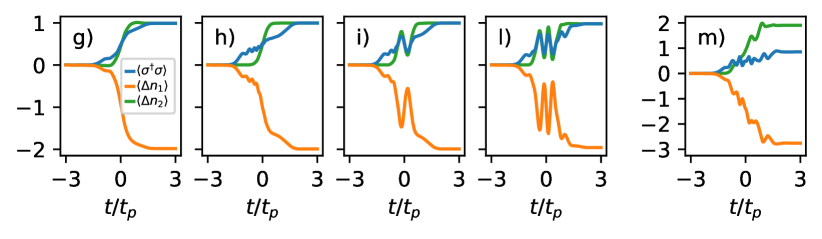
Figure 1: (a–f): Quantum state of the coupled emitter-field system after a SUPER pulse, as a function of the detuning $\Delta_{2}=t_{p}\delta_{2}$ and the initial number of photons $n_{2}^{\rm i}$ in mode 2. The system is initialized at time $t_{\rm i}$ in the state $\ket{G,n_{1}^{\rm i},n_{2}^{\rm i}}$, with $\ket{n_{j}^{\rm i}}$ representing Fock states. The quantities plotted are the final excited state population $\expectationvalue{\sigma^{\dagger}\sigma}$ (panels a, b) and the variation $\expectationvalue{\Delta n_{j}}=\expectationvalue{a_{j}^{\dagger}a_{j}(t_{\rm f})}-n_{j}^{\rm i}$ of the average photon number in mode 1 (c, d) and 2 (e, f). (g–m): Evolution of $\expectationvalue{\sigma^{\dagger}\sigma}$, $\expectationvalue{\Delta n_{1}}$, and $\expectationvalue{\Delta n_{2}}$ for different configurations corresponding to local maxima in panels a and b, see red arrows. Parameters for the first mode are fixed at $\Delta_{1}=6$ (everywhere), $\sqrt{n_{1}^{\rm i}}=62.83$ (panels a, c, e), and $\sqrt{n_{1}^{\rm i}}=157.08$ (panels b, d, f). The dimensionless interaction strength is $G_{1}=G_{2}=0.1$ (everywhere).

We begin by considering the system dynamics when the field modes are both red-detuned with respect to the emitter and initialized in large-number Fock states $\ket{n_{j}^{\rm i}}$. This is motivated by the fact that optical excitation of a quantum emitter involves laser pulses with a large number of photons. Although Fock states are generally inaccurate to describe the quantum field of a laser, their use allows for a substantial numerical simplification of the problem in terms of the number $M_{j}$ of states needed. The case of coherent states, which represent a more accurate description of the laser field, will be examined later in Section 6, where we find good qualitative agreement between the two pictures. We note that the dynamics is governed by the dimensionless quantities $\Delta_{j}=t_{p}\delta_{j}$, and $G_{j}=t_{p}g_{j}$, and we will discuss the results in terms of these parameters.

In Fig. 1, we explore the population $P_{X}=\expectationvalue{\sigma^{\dagger}\sigma}$ of the $\ket{X}$ state and of both field modes at time $t_{\rm f}=3t_{p}$, i.e. after interaction has occurred. Following the literature [8, 9, 12, 13], we fix the parameters for the first mode (dimensionless detuning $\Delta_{1}=t_{p}\delta_{1}$ and initial photon number $n_{j}^{\rm i}$), and scan the corresponding parameters for the second mode. Note that the terms “first” and “second” identify the mode with shorter and larger detuning in absolute value, respectively. In the SUPER scheme literature based on semiclassical models of light-matter interaction, results are typically shown as a function of the electric field amplitude [7, 12], which is proportional to the square root of the photon number. Therefore, we choose to plot the results as a function of $\sqrt{n_{2}^{\rm i}}$. The dimensionless coupling is fixed to $G_{1}=G_{2}=0.1$.

In Fig. 1a, which is taken at fixed $\sqrt{n_{1}^{\rm i}}=62.83$ ($n_{1}^{\rm i}=3947$), we identify a region of near-unity exciton preparation fidelity, with a maximum of $P_{X}=0.99$. This is accompanied by additional resonances at shorter detuning with incomplete population inversion of the order of $\approx 0.4$ at maximum. In contrast, by increasing the initial photon number in mode 1 to $\sqrt{n_{1}^{\rm i}}=157.08$ ($n_{1}^{\rm i}=24673$), we observe multiple resonances with $P_{X}\geq 0.99$ (see Fig. 1b). Similar features have been observed in the literature using a classical description of the field and represent the signature of the SUPER scheme. We conclude that our model of a two-level emitter interacting with two quantized field modes captures the physics of the SUPER swing-up effect satisfactorily.

Differently from the semiclassical description, a quantized model give access to the exact number of photons in each mode. We thus calculate the difference $\expectationvalue{\Delta n_{j}}=\expectationvalue{a_{j}^{\dagger}a_{j}(t_{\rm f})}-\expectationvalue{a_{j}^{\dagger}a_{j}(t_{\rm i})}$ of the photon number in each mode before and after interaction, which is plotted in Fig. 1c–f. In correspondence with each resonance of $P_{X}$, we observe variations of the photon number in both modes. Remarkably, mode 1 shows always a decrease in photon number, whereas mode 2 shows an unexpected increase. Exploring the dynamics in correspondence of $P_{X}\approx 1$ (see Fig. 1g–l), we find that exactly two photons are subtracted from mode 1, while mode 2 gains one photon in the process. This demonstrates surprisingly that SUPER scheme is a multi-photon process involving a redistribution of photons between the field modes. We also identify a higher-order process leading to large but incomplete population inversion $P_{X}>0.85$ (see Fig. 1m) where almost three photons ($\expectationvalue{\Delta n_{1}}=-2.76$) are subtracted from mode 1, while mode 2 gains almost two photons ($\expectationvalue{\Delta n_{2}}=1.90$). We hypothesize that a process leading to $\expectationvalue{\Delta n_{1}}=-3$ and $\expectationvalue{\Delta n_{2}}=2$ exactly might be found with a thorough investigation of the parameter space, which is not performed here. Despite these variations in the photon number, we observe that the total excitation number $\mathcal{N}=\sigma^{\dagger}\sigma+a_{1}^{\dagger}a_{1}+a_{2}^{\dagger}a_{2}$ is indeed conserved in the process, i.e. $P_{X}+\expectationvalue{\Delta n_{1}}+\expectationvalue{\Delta n_{2}}=0$.

In contrast with the semiclassical description of the SUPER scheme dynamics, which shows fast and ample oscillations in time of the $\ket{X}$ state population within one pulse (of the order of 10–30), the first leftmost resonance in Fig. 1a–b is characterized by a smooth and monotonic dynamics. Higher order resonances at shorter detuning and larger photon number display few oscillations in the emitter population and photon number of the field modes (of the order of 2–3).

4 Dynamics of the red-and-blue dichromatic scheme

In the red-and-blue dichromatic scheme, two laser pulses are symmetrically detuned to the red and blue side of the spectrum with respect to the emitter. It has been demonstrated that specific configurations involving pulses of different amplitude generate complete population inversion, whereas symmetric configurations with identical pulse amplitude lead necessarily to $P_{X}=0$ [18]. Exciton preparation with the red-and-blue scheme occurs through a similar swing-up effect of the population [18, 12].

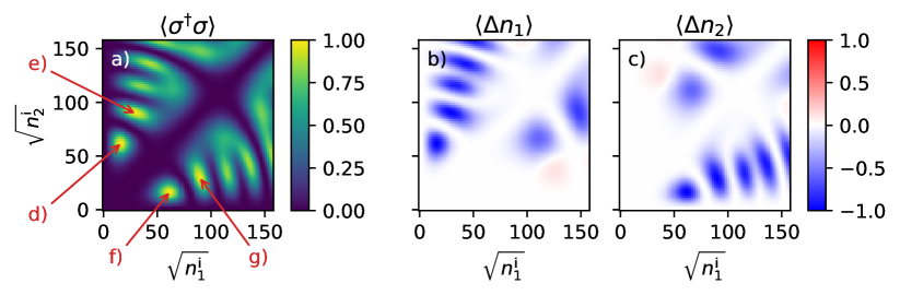
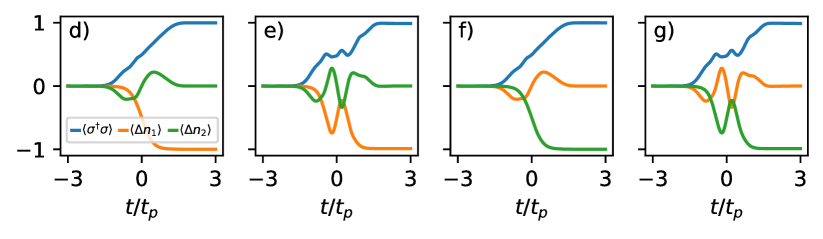
Figure 2: (a, b, c): Quantum state of the coupled emitter-field system after a red-and-blue dichromatic pulse, as a function of the initial number of photons $n_{j}^{\rm i}$ in each mode $j$. The system is initialized in the state $\ket{G,n_{1}^{\rm i},n_{2}^{\rm i}}$, with $\ket{n_{j}^{\rm i}}$ representing Fock states. The quantities plotted are the final $\ket{X}$ state population $\expectationvalue{\sigma^{\dagger}\sigma}$ (panel a) and the variations $\expectationvalue{\Delta n_{j}}=\expectationvalue{a_{j}^{\dagger}a_{j}(t_{\rm f})}-n_{j}^{\rm i}$ of the average photon numbers in modes 1 (b) and 2 (c). (d–g): Evolution of $\expectationvalue{\sigma^{\dagger}\sigma}$, $\expectationvalue{\Delta n_{1}}$, and $\expectationvalue{\Delta n_{2}}$ in time for different configurations corresponding red arrows in panel a. In all panels, the mode detunings are fixed at $\Delta_{1}=-\Delta_{2}=6$, and the dimensionless interaction strength is $G_{1}=G_{2}=0.1$.

To model this scenario, we constrain the detuning to $\Delta_{1}=-\Delta_{2}=6$ and explore the dependence of the final exciton population as a function of the initial photon number in each mode. Once again, we initialize the field modes in Fock states $\ket{n_{j}^{\rm i}}$. As shown in Fig. 2a, we obtain several resonances featuring $P_{X}\approx 1$ in quantitative agreement with results based on semiclassical models [12]. No resonance is indeed observed along the diagonal $n_{1}^{\rm i}=n_{2}^{\rm i}$, in agreement with the requirement of different pulse amplitudes.

In contrast with the SUPER scheme, we observe that this process involves photon exchange with a single mode, see Figs. 2b and Fig. 2c. For example, at $\quantity(\sqrt{n_{1}^{\rm i}},\sqrt{n_{2}^{\rm i}})$ = (16.00, 61.25) and (29.21, 89.84), exactly one photon is subtracted from mode 1 (the one at positive detuning) to populate the excited state, while no photon exchange occurs with mode 2 (negative detuning). The opposite holds true by exchanging $n_{1}^{\rm i}$ with $n_{2}^{\rm i}$. There, one photon is subtracted from mode 2 with no gain/loss in mode 1. We notice, however, that in both cases the mode with $\expectationvalue{\Delta n_{j}}=0$ participates actively in the dynamics, as demonstrated by oscillations of the average photon number in time reported in Fig. 2d–g.

Similarly to the SUPER scheme, we notice that the fundamental resonance (namely, the one occurring at smaller photon number) shows a monotonic increase in $P_{X}$ with no oscillations (Fig. 2d–g). Higher order resonances display few small oscillations.

5 Strong emitter-field coupling: “vacuum” swing-up

So far, the emitter dynamics under a two-color excitation protocol involving a large number of photons is consistent with a semiclassical approach where the electromagnetic field is treated as a classical object. We now explore a truly quantum regime where the field modes are populated by a few photons only.

The strength of the emitter-field coupling is governed by the coupling constants $G_{j}$ and the electric field amplitude $E_{j}\propto\sqrt{n_{j}^{\rm i}}$, as one can readily verify by calculating the matrix elements of $H_{\rm int}$. Therefore, to maintain the same effective light-matter coupling while scaling down the field occupation to the few photon regime, we simultaneously increase the value of the dimensionless coupling constants $G_{j}=t_{p}g_{j}$. In experiments, this can be done by increasing the emitter-field coupling $g_{j}$ via optical engineering of the electromagnetic environment, or by increasing the pulse duration $t_{p}$.

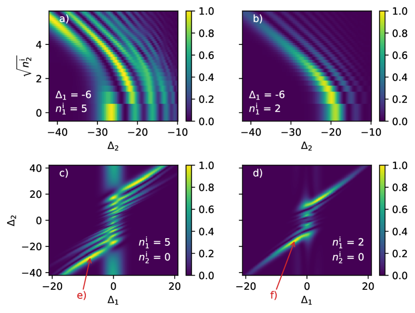
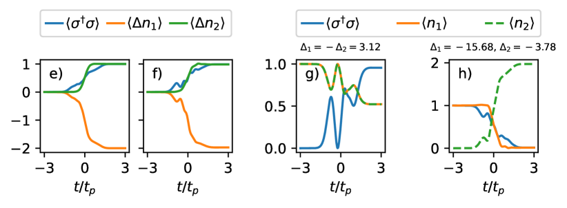
Figure 3: (a–d): Final $\ket{X}$ state population $\expectationvalue{\sigma^{\dagger}\sigma}$ after a SUPER pulse in the low photon number regime. The system is initialized in the state $\ket{G,n_{1}^{\rm i},n_{2}^{\rm i}}$, with $\ket{n_{j}^{\rm i}}$ representing Fock states. In (a) and (b), the detuning $\Delta_{1}$ and initial number of photons $n_{1}^{\rm i}$ in mode 1 are fixed as reported in the Figure, $\Delta_{2}$ is varied continuously along the $x$-axis, and $n_{2}^{\rm i}$ is varied in integer steps along the $y$-axis. In (c) and (d), the initial photon numbers $n_{j}^{\rm i}$ are fixed and the detunings $\Delta_{j}$ are varied continuously. (e, f): Evolution of $\expectationvalue{\sigma^{\dagger}\sigma}$, $\expectationvalue{\Delta n_{1}}$, and $\expectationvalue{\Delta n_{2}}$ in time for different configurations corresponding red arrows in panels c) and d). (g): Evolution of $\expectationvalue{\sigma^{\dagger}\sigma}$, $\expectationvalue{n_{1}}$, and $\expectationvalue{n_{2}}$ in time for a red-and-blue dichromatic configuration with $\Delta_{1}=-\Delta_{2}=3.12$. (h): Evolution of $\expectationvalue{\sigma^{\dagger}\sigma}$, $\expectationvalue{n_{1}}$, and $\expectationvalue{n_{2}}$ in time for a SUPER configuration with $\Delta_{1}=-15.68$, $\Delta_{2}=-3.78$, and where the emiter is initially in the excited state $\ket{X}$. Note that panels g) and h) report the absolute photon numbers $\expectationvalue{n_{j}}$ rather than the variation $\expectationvalue{\Delta n_{j}}$. In all panels, the dimensionless interaction strength is $G_{1}=G_{2}=5$.

Starting with the SUPER scheme, we explore this scenario in Fig. 3 by increasing the coupling to $G_{1}=G_{2}=5$ and scaling the initial number of photons in mode 1 down to $n_{1}^{\rm i}=5$ and $n_{1}^{\rm i}=2$ (panels a and b, respectively). Interestingly, we observe that the typical resonances of the SUPER scheme are still clearly visible, and only few photons are needed to achieve full population inversion. Quite surprisingly, exciton preparation is still possible even when the second field mode is prepared in the vacuum state $n_{2}^{\rm i}=0$. We observe $P_{X}=0.97$ for $(n_{1}^{\rm i},n_{2}^{\rm i})=(5,0)$ and $P_{X}=0.88$ for $(n_{1}^{\rm i},n_{2}^{\rm i})=(2,0)$, where incomplete population inversion $P_{X}<1$ is explained by the fact that we have chosen an arbitrary value of $\Delta_{1}=-6$. By fixing the initial number of photons in each mode and continuously varying both detunings $\Delta_{j}$, we obtain indeed full population inversion with $P_{X}=1.00$ at $(n_{1}^{\rm i},n_{2}^{\rm i},\Delta_{1},\Delta_{2})=(5,0,-7.56,-28.56)$, and $P_{X}=0.99$ at $(n_{1}^{\rm i},n_{2}^{\rm i},\Delta_{1},\Delta_{2})=(2,0,-4.06,-15.96)$, see Figs. 3c and d. The corresponding time-dependent dynamics is plotted in Figs. 3e and f, demonstrating that full population inversion with exchange of multiple photons in indeed possible even when one of the field modes is in the vacuum state. For the case of Fig. 3f, where the field is initialized in $(n_{1}^{\rm i},n_{2}^{\rm i})=(2,0)$, we notice that mode 1 is left in the vacuum state, while mode 2 is in the single-photon Fock state $\ket{n_{2}^{\rm f}}=\ket{1}$ after interaction.

We observe no population inversion when $(n_{1}^{\rm i},n_{2}^{\rm i})=(1,0)$, for any value of the detunings. This demonstrates that the minimum excitation number to activate the SUPER mechanism is $\mathcal{N}=2$, consistent with the fact that the SUPER scheme cannot be explained with the exchange of one single photon between the emitter and the field.

Applying similar considerations, we find signatures of the red-and-blue dichromatic scheme in the few-photon regime as well. Despite the fact that dichromatic excitation in the large photon number regime is explained with the subtraction of a single photon from one of the modes, we do not observe population inversion for initial state $(n_{1}^{\rm i},n_{2}^{\rm i})=(1,0)$ or $(0,1)$, indicating that the requirement on the excitation number is still $\mathcal{N}\geq 2$. On the other hand, we find that preparing the field modes in two single-photon states $\quantity(n_{1}^{\rm i},n_{2}^{\rm i})=(1,1)$ at detuning $\Delta_{1}=-\Delta_{2}=3.12$ leads to population of the exciton state with fidelity $P_{X}=0.96$, see Fig. 3g. Here, the system is approximately left in the entangled state $\ket{\psi(t_{\rm f})}=\frac{1}{\sqrt{2}}\quantity(\ket{X,1,0}+\ket{X,0,1})$ after interaction, meaning that half a photon has been subtracted from both modes on average.

Finally, it is worth noting that the multi-photon resonances of the SUPER scheme work in the reverse fashion as well. In other words, it is possible to completely depopulate an initially excited emitter by subtracting one excitation from mode 1, while increasing the population of the other field mode by two excitations. This may be used to engineer non-linear interaction between field modes at different frequency. For example, as shown in Fig. 3h, a single-photon state at detuning $\Delta_{1}=-15.68$ is converted into a two-photon state at $\Delta_{2}=-3.78$ accompanied by relaxation of the emitter to the ground state.

6 Coherent states

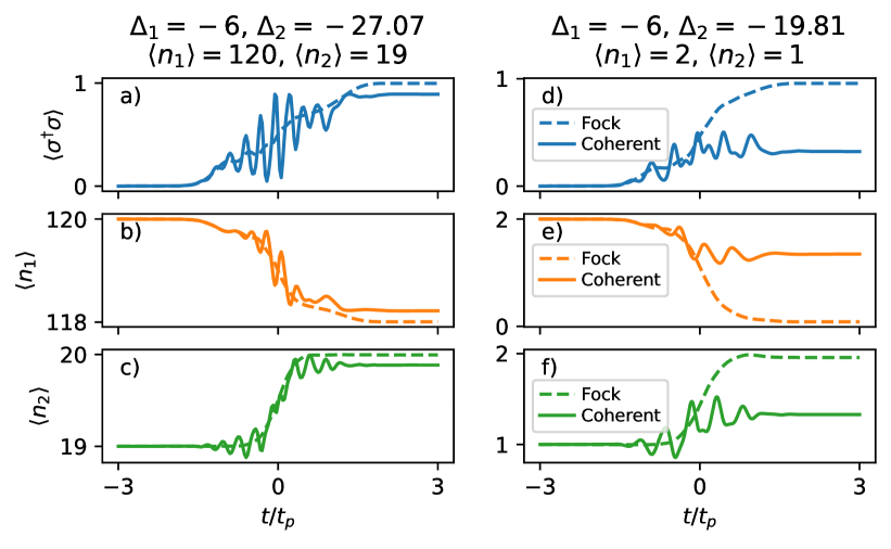
Figure 4: Evolution of $\expectationvalue{\sigma^{\dagger}\sigma}$, $\expectationvalue{n_{1}}$, and $\expectationvalue{n_{2}}$ in time for different initial states of the electromagnetic field. The field modes are initialized either in Fock states containing $n_{1}^{\rm i}$ and $n_{2}^{\rm i}$ photons respectively (dashed lines), or in coherent states with the same average number of photons (solid lines). Detunings $\Delta_{j}$ and initial photon numbers $n_{j}^{\rm i}$ are indicated in the top panel title. The dimensionless interaction strength is $G_{1}=G_{2}=1$ (a–c) and $G_{1}=G_{2}=5$ (d–f).

So far we have considered Fock states of the field modes for simplicity. However, the quantum state of a laser pulse is best described by a coherent state $\ket{\alpha}=e^{-|\alpha^{2}|/2}\sum_{n}\alpha^{n}/(\sqrt{n!})\ket{n}$. In Fig. 4, we compare the dynamics for a case where the field is initialized in the multi-mode Fock state $\ket{n_{1}^{\rm i},n_{2}^{\rm i}}$ with the case where the initial field state is $\ket{\alpha_{1}^{\rm i},\alpha_{2}^{\rm i}}$, with $\ket{\alpha_{j}^{\rm i}}$ representing coherent states containing the same number of photons $\matrixelement{\alpha_{j}^{\rm i}}{a_{j}^{{\dagger}}a_{j}}{\alpha_{j}^{\rm i}}=|\alpha_{j}^{\rm i}|^{2}=n_{j}^{\rm i}$ on average. For sufficiently high excitation number (see Fig. 4a–c), we observe that the two situations are qualitatively similar. Indeed, the description based on coherent states confirms that the SUPER scheme excitation takes place by removing approximately two photons from mode 1 while simultaneously increasing the population of mode 2 by one photon. However, whereas the Fock state description yields a monotonic dynamics, the coherent state model reproduces the typical swing-up pattern that characterizes the SUPER scheme, resulting in fast oscillations of the exciton population. Despite this remarkable qualitative difference, the attained value of $P_{X}$ using coherent states is quantitatively similar to the one obtained using Fock states.

However, the agreement breaks down in the deep quantum regime of low excitation number. As shown in Figs. 4d–f, a model using coherent states predicts $P_{X}=0.32$ for $(|\alpha_{1}^{\rm i}|^{2},|\alpha_{2}^{\rm i}|^{2})=(2,1)$ and $(\Delta_{1},\Delta_{2})=(-6,-19.81)$, while the value predicted with a Fock state assumption is $P_{X}=0.96$. We conclude that SUPER scheme excitation in the low photon number regime necessitates of few-photon Fock states as compared with coherent states of small amplitude. Whereas the latter can be realized, for example, with attenuated laser pulses, the former are fundamentally different and more challenging to realize [22, 23, 24].

7 Discussion

We have investigated the physics of two-color excitation schemes in terms of energy exchanges between the emitter and the laser pump. To do so, we have developed a model for a two-level emitter interacting with two quantized field modes, where interaction occurs during short pulses of duration $t_{p}$ in time. Both the SUPER and the red-and-blue dichromatic schemes have been considered.

We have observed that exciton population under the SUPER scheme, where both modes are red-detuned with respect to the emitter, is accompanied by variations in the photon number of both modes, unveiling the multi-photon nature of this process. We find clear signatures of events with $(\expectationvalue{\sigma^{\dagger}\sigma},\expectationvalue{\Delta n_{1}},\expectationvalue{\Delta n_{2}})=(+1,-2,+1)$ and $(+1,-3,+2)$, where multiple excitations are subtracted from the 1st field mode (the one with smaller detuning, in absolute value). While one excitation is used to raise the emitter population to the excited state, the remaining are absorbed by the 2nd field mode at larger detuning. Interestingly, this holds true in the regime where the field modes are populated with only few photons, and even when one of the field is in the vacuum state. We speculate that events involving exchange of higher number of photons, i.e. $(\expectationvalue{\sigma^{\dagger}\sigma},\expectationvalue{\Delta n_{1}},\expectationvalue{\Delta n_{2}})=(1,-m,m-1)$ with $m>3$, might be found at larger total power, although we have not observed such a case in this work.

This finding is in stark contrast with the paradigm of resonant excitation, where the emitter exchanges one energy quantum with a single field mode. We have indeed verified that our model reproduces this scenario by removing the 2nd field mode (i.e. setting $G_{2}=0$) and moving the 1st mode into resonance with the emitter ($\Delta_{1}=0$). By scanning the initial number of photons $n_{1}^{\rm i}$ in mode 1, we have found clear signatures of Rabi oscillations. For configurations resulting in $P_{X}=1$, we have observed that one single photon is removed from the field. A similar scenario is expected to take place in phonon-assisted excitation [25, 26, 27], although we have not included phonon coupling in this work.

Reversing the working principle of the SUPER scheme, our model shows that it is possible to stimulate emission from an excited emitter with a simultaneous redistribution of photons among the field modes. For instance, a system initialized in the state $\ket{X,n_{1},n_{2}}$ is found in the state $\ket{G,n_{1}-1,n_{2}+2}$ after interaction with two red-detuned modes. Once again, this is valid in the case $n_{2}=0$ where mode 2 is in the vacuum state. Quite interestingly, this observation challenges the typical paradigm of spontaneous emission stating that the emitted photon must have the same frequency as the photons in the incident wave. These findings may be used to engineer a non-linear interaction where one single photon stimulates the emission of two identical photons at a different frequency.

Considering the red-and-blue dichromatic excitation, where one of the field modes is moved to the blue side of the spectrum, we have observed that it involves energy exchange with only one of the field modes. However, our results demonstrate that the presence of a second field mode is necessary to engineer full population inversion, even when no variation in its the photon number is recorded. An exception to this paradigm is the case of dichromatic excitation for an initial state $\ket{G,1,1}$, where we find that half a photon is subtracted on average from both modes.

It is worth noting that we have obtained a good qualitative agreement with the description of the SUPER and red-and-blue dichromatic scheme under a semiclassical model for light-matter interaction, where the field is not quantized. However, the advantage of the quantum model presented here is that it makes it possible to calculate the variation in photon number for each mode. We have furthermore observed that a description of the laser field in terms of coherent states is needed to reproduce the typical swing-up behavior of the excited state population under SUPER scheme excitation, which is characterized by fast oscillations. However, we have surprisingly found that a description in term of Fock states yields qualitatively similar results for the final population inversion, and demands less computational resources. For example, the Fock state dynamics shown in Fig. 4a is fully converged when using $M_{1}=M_{2}=11$ states in the field Hilbert space, whereas $M_{1}=M_{2}=91$ states are required for full convergence of the corresponding coherent state simulation. The qualitative agreement between the two descriptions is however limited to the large photon number regime. For small photon numbers of the order of few units, fundamental differences in the behavior of Fock and coherent states emerge.

Finally, we have used values in the range 0.1–5 for the dimensionless coupling constants $G_{j}=g_{j}t_{p}$. Considering short pulses of the order of $t_{p}=$ 2–3 ps, a value $G_{j}=0.1$ is obtained with a light-matter coupling strength of the order of $g_{j}=$ 0.03–0.05 THz. The latter corresponds to typical values attained in high-Q micropillars [28, 12] or open tunable microcavities [6], and similar values are found elsewhere in the literature [26]. Two strategies may be pursued to attain stronger dimensionless coupling $G_{j}=5$. On one hand, the pulse duration may be increased by one order of magnitude to $t_{p}\approx 100$ ps. We notice, however, that the system in this regime is more prone to environment induced decoherence, such as charge and spin noise, and phonon scattering. It has been shown that the latter is especially detrimental for the SUPER scheme, leading to reduced population inversion [12, 13]. As alternative, a light-matter coupling strength $g_{j}\approx 2$ THz is needed to obtain $G_{j}=5$. Whereas such a strong coupling maybe challenging to realize, we notice that nanocavities with extreme photon confinement well below the diffraction limit in dielectrics have been designed and fabricated in silicon [29]. Here, ultra-strong light-matter coupling is expected due to the extremely low mode volume.

As mentioned, phonon scattering is generally detrimental to the SUPER scheme. Here, we have considered an ideal case of unitary dynamics with no decoherence, where the Schrödinger equation is solved exactly with a numerical algorithm to obtain the quantum state $\ket{\psi(t)}$ of the emitter-field system. To include phonon coupling, a master equation description in terms of the density operator $\rho$ is needed. However, the quantum state $\ket{\psi}$ is implemented numerically as a vector with dimension $2M_{1}M_{2}$. Using the same basis, the density operator $\rho$ becomes a $2M_{1}M_{2}\times 2M_{1}M_{2}$ matrix, which poses serious numerical challenges due to the substantial increase in computational resources.

During the writing of this manuscript, we became aware of a related work which also demonstrates the multi-photon nature of the SUPER scheme [30].

8 Conclusions

We have studied the exchange of energy between a two-level emitter and two quantized field modes under the SUPER scheme excitation. Surprisingly, we have found that one mode loses two or more photons while the other gains at least one, proving that the SUPER is a multi-photon process involving a redistribution of photons between the field modes. Our results unveil a novel and unexpected off-resonant interaction of light and matter, and open new possibilities for manipulating the quantum state of atoms using only few off-resonant photons.

Funding This work received supported from the European Research Council (ERC-CoG “Unity”, grant no.865230) and the European Union’s Horizon 2020 Research and Innovation Programme under the Marie Skłodowska-Curie Grant (Agreement No. 861097).

Disclosures The authors declare no conflicts of interest.

Data availability Data underlying the results presented in this paper may be obtained from the authors upon reasonable request.

References

- [1] T. Heindel, J.-H. Kim, N. Gregersen, et al., “Quantum dots for photonic quantum information technology,” \JournalTitleAdv. Opt. Photon. 15, 613–738 (2023).
- [2] N. Maring, A. Fyrillas, M. Pont, et al., “A versatile single-photon-based quantum computing platform,” \JournalTitleNat. Photon. 18, 603–609 (2024).
- [3] C. Joshi, A. Farsi, S. Clemmen, et al., “Frequency multiplexing for quasi-deterministic heralded single-photon sources,” \JournalTitleNat. Commun. 9, 847 (2018).
- [4] F. Kaneda and P. G. Kwiat, “High-efficiency single-photon generation via large-scale active time multiplexing,” \JournalTitleSci. Adv. 5, eaaw8586 (2019).
- [5] H. Wang, Y. M. He, T. H. Chung, et al., “Towards optimal single-photon sources from polarized microcavities,” \JournalTitleNat. Photonics 13, 770–775 (2019).
- [6] N. Tomm, A. Javadi, N. O. Antoniadis, et al., “A bright and fast source of coherent single photons,” \JournalTitleNat. Nanotechnol. 16, 399–403 (2021).
- [7] T. K. Bracht, M. Cosacchi, T. Seidelmann, et al., “Swing-up of quantum emitter population using detuned pulses,” \JournalTitlePRX Quantum 2, 040354 (2021).
- [8] Y. Karli, F. Kappe, V. Remesh, et al., “Super scheme in action: Experimental demonstration of red-detuned excitation of a quantum emitter,” \JournalTitleNano Lett. 22, 6567 (2022).
- [9] K. Boos, F. Sbresny, S. K. Kim, et al., “Coherent swing-up excitation for semiconductor quantum dots,” \JournalTitleAdvanced Quantum Technologies 7, 2300359 (2024).
- [10] N. Heinisch, N. Köcher, D. Bauch, and S. Schumacher, “Swing-up dynamics in quantum emitter cavity systems: Near ideal single photons and entangled photon pairs,” \JournalTitlePhys. Rev. Res. 6, L012017 (2024).
- [11] R. Joos, S. Bauer, C. Rupp, et al., “Triggered telecom C-band single-photon source with high brightness, high indistinguishability and sub-GHz spectral linewidth,” arXiv:2310.20647.
- [12] L. Vannucci and N. Gregersen, “Highly efficient and indistinguishable single-photon sources via phonon-decoupled two-color excitation,” \JournalTitlePhys. Rev. B 107, 195306 (2023).
- [13] L. Vannucci, J. Ferreira Neto, C. Piccinini, et al., “Single-photon emitters in : Critical role of phonons on excitation schemes and indistinguishability,” \JournalTitlePhys. Rev. B 109, 245304 (2024).
- [14] T. K. Bracht, T. Seidelmann, T. Kuhn, et al., “Phonon Wave Packet Emission during State Preparation of a Semiconductor Quantum Dot using Different Schemes,” \JournalTitlePhys. Status Solidi B 259, 2100649 (2022).
- [15] M. Kuniej, M. Gawełczyk, and P. Machnikowski, “Hybrid acousto-optical swing-up preparation of exciton and biexciton states in a quantum dot,” arXiv:2402.07887.
- [16] C. Güney Torun, M. Gökçe, T. K. Bracht, et al., “SUPER and subpicosecond coherent control of an optical qubit in a tin-vacancy color center in diamond,” arXiv:2312.05246.
- [17] T. K. Bracht, T. Seidelmann, Y. Karli, et al., “Dressed-state analysis of two-color excitation schemes,” \JournalTitlePhys. Rev. B 107, 035425 (2023).
- [18] Z. X. Koong, E. Scerri, M. Rambach, et al., “Coherent dynamics in quantum emitters under dichromatic excitation,” \JournalTitlePhys. Rev. Lett. 126, 047403 (2021).
- [19] J. Gruver, J. Aliaga, H. A. Cardeira, and A. Proto, “Exact solution of the generalized time-dependent jaynes-cummings hamiltonian,” \JournalTitlePhysics Letters A 178, 239–244 (1993).
- [20] A. Joshi and S. V. Lawande, “Generalized jaynes-cummings models with a time-dependent atom-field coupling,” \JournalTitlePhys. Rev. A 48, 2276–2284 (1993).
- [21] A. Dasgupta, “An analytically solvable time-dependent jaynes-cummings model,” \JournalTitleJournal of Optics B: Quantum and Semiclassical Optics 1, 14 (1999).
- [22] M. Cooper, L. J. Wright, C. Söller, and B. J. Smith, “Experimental generation of multi-photon Fock states,” \JournalTitleOpt. Express 21, 5309–5317 (2013).
- [23] M. Uria, P. Solano, and C. Hermann-Avigliano, “Deterministic Generation of Large Fock States,” \JournalTitlePhys. Rev. Lett. 125, 093603 (2020).
- [24] T. Sonoyama, K. Takahashi, T. Sano, et al., “Generation of multi-photon Fock states at telecommunication wavelength using picosecond pulsed light,” arXiv:2405.06567.
- [25] M. Cosacchi, F. Ungar, M. Cygorek, et al., “Emission-Frequency Separated High Quality Single-Photon Sources Enabled by Phonons,” \JournalTitlePhys. Rev. Lett. 123, 017403 (2019).
- [26] C. Gustin and S. Hughes, “Efficient pulse-excitation techniques for single photon sources from quantum dots in optical cavities,” \JournalTitleAdvanced Quantum Technologies 3, 1900073 (2020).
- [27] S. E. Thomas, M. Billard, N. Coste, et al., “Bright polarized single-photon source based on a linear dipole,” \JournalTitlePhys. Rev. Lett. 126, 233601 (2021).
- [28] B.-Y. Wang, E. V. Denning, U. M. Gür, et al., “Micropillar single-photon source design for simultaneous near-unity efficiency and indistinguishability,” \JournalTitlePhys. Rev. B 102, 125301 (2020).
- [29] M. Albrechtsen, B. Vosoughi Lahijani, R. E. Christiansen, et al., “Nanometer-scale photon confinement in topology-optimized dielectric cavities,” \JournalTitleNat. Commun. 13, 6281 (2022).
- [30] Q. W. Richter, J. M. Kaspari, T. K. Bracht, et al., “Few-photon super: Quantum emitter inversion via two off-resonant hoton modes,” arXiv:2405.20095.