SKD-TSTSAN: Three-Stream Temporal-Shift Attention Network Based on Self-Knowledge Distillation for Micro-Expression Recognition

Abstract

Micro-expressions (MEs) are subtle facial movements that occur spontaneously when people try to conceal the real emotions. Micro-expression recognition (MER) is crucial in many fields, including criminal analysis and psychotherapy. However, MER is challenging since MEs have low intensity and ME datasets are small in size. To this end, a three-stream temporal-shift attention network based on self-knowledge distillation (SKD-TSTSAN) is proposed in this paper. Firstly, to address the low intensity of ME muscle movements, we utilize learning-based motion magnification modules to enhance the intensity of ME muscle movements. Secondly, we employ efficient channel attention (ECA) modules in the local-spatial stream to make the network focus on facial regions that are highly relevant to MEs. In addition, temporal shift modules (TSMs) are used in the dynamic-temporal stream, which enables temporal modeling with no additional parameters by mixing ME motion information from two different temporal domains. Furthermore, we introduce self-knowledge distillation (SKD) into the MER task by introducing auxiliary classifiers and using the deepest section of the network for supervision, encouraging all blocks to fully explore the features of the training set. Finally, extensive experiments are conducted on four ME datasets: CASME II, SAMM, MMEW, and CAS(ME)³. The experimental results demonstrate that our SKD-TSTSAN outperforms other existing methods and achieves new state-of-the-art performance. Our code will be available at https://github.com/GuanghaoZhu663/SKD-TSTSAN.

[a]organization=MOEMIL Laboratory, School of Optoelectronic Science and Engineering,addressline=University of Electronic Science and Technology of China, city=Chengdu, postcode=611731, country=China [b]organization=School of Optoelectronic Science and Engineering,addressline=University of Electronic Science and Technology of China, city=Chengdu, postcode=611731, country=China [c]organization=UESTC-MIT Joint Institute of Intelligent Microtechnique,city=Yibin, postcode=644000, country=China

1 Introduction

Facial expression (FE) is a common means of nonverbal communication and is crucial for understanding human mental states and intentions [1]. Facial expressions can generally be categorized into two classes: macro-expressions and micro-expressions (MEs). The major variations between them are intensity and duration. Macro-expressions typically have a duration of 0.5-4 seconds and involve muscle movements covering a large area of the face, which can easily be recognized by humans [2]. In contrast, MEs reflect hidden emotions that come out spontaneously when people strive to hide their true emotions. It usually lasts only 1/25 to 1/3 of a second with muscle movements in a minor region of the face [3], which is difficult to recognize, and only an expert with extensive training can distinguish MEs. MEs are significant in many fields, such as crime analysis [4], emotional communication, and clinical diagnosis. Therefore, researchers are striving to utilize computer vision techniques for automatic micro-expression recognition (MER).

Early MER methods are based on manual feature extraction, such as Local Binary Pattern histograms from Three Orthogonal Planes (LBP-TOP) [5] and Main Directional Mean Optical-flow (MDMO) [6]. These methods largely rely on manually designed extractors and complicated parameter adjustments. The extracted features are mainly low-level features [1], therefore it is difficult to recognize the subtle movements in MEs with high accuracy. With the proposal of a series of ME datasets [7, 8, 9, 10] and the development of deep learning, researchers began to use CNN to extract spatial and temporal features of MEs. For example, Song et al. [11] proposed a three-stream convolutional neural network (TSCNN) to learn the spatiotemporal information of MEs. Xia et al. [12] trained two dual-stream baseline models called MiNet and MaNet using the ME dataset and macro-expression dataset. By introducing two auxiliary tasks between the two models, MiNet can effectively extract both the dynamic patterns of the muscle motion and the static texture of the face. Although these methods can extract ME features and achieve promising results, there are still two major challenges in MER: the low intensity of MEs and overfitting on small ME datasets [9]. Since MEs have low intensity, networks need to have strong representation ability, which generally means more convolutional layers and computational costs. However, complex models usually overfit on small-scale ME datasets. Therefore, in order to mine subtle ME motions from small ME datasets, more effective blocks need be introduced.

To address the above challenges, we propose a three-stream temporal-shift attention network based on self-knowledge distillation called SKD-TSTSAN in this paper. Firstly, we use the TSCNN [11] as our baseline, which consists of three streams, namely static-spatial stream (S-stream), local-spatial stream (L-stream), and dynamic-temporal stream (T-stream). The inputs of the three streams are the whole facial image, the concatenation of $n\times n$ localized facial images, and optical flow images, respectively. The three recognition streams are finally fused into a fully connected layer for MER tasks. Targeting the low intensity of MEs, we add pre-trained magnification networks [13] to the head of each convolutional stream based on transfer learning. For an end-to-end framework, a magnification network without an encoder is employed. Since ME only appears in local regions of the face, we incorporate efficient channel attention (ECA) modules [14] into the L-stream to encourage the network to focus on significant local regions.

Compared with 2D CNNs, 3D CNNs can mine the spatiotemporal information of videos more effectively [1]. However, 3D CNNs generally have a large number of parameters and are easily overfitted on small-scale ME datasets [1]. To capture temporal relations in ME sequences and maintain the complexity of 2D CNNs, we introduce temporal shift modules (TSMs) [15] in T-stream. In TSM, part of the optical flow features’ channels are shifted along the temporal dimension to realize the information exchange. Moreover, to further enhance the performance of the lightweight network, the macro-expression dataset CK+ [16] is employed for pre-training, and self-knowledge distillation (SKD) [17] is incorporated. Additional convolutional and fully connected layers are added to form multiple auxiliary classifiers (ACs). By using labels and the model’s final output to train the ACs, we enable all of the model’s blocks to fully explore the training set’s features.

In summary, the main contributions of this paper are as follows:

• A motion magnification network is employed to increase the intensity of ME muscle motion, making the features of apex frames and optical flow fields more obvious.

• ECA modules are introduced in the local-spatial stream to ignore redundant information and focus on more meaningful channels. TSMs are added in the dynamic-temporal stream, which achieves information exchange in the temporal dimension with no additional parameters.

• We explore the effectiveness of self-knowledge distillation on the MER tasks, introducing auxiliary classifiers in the network to enable comprehensive learning of features from the training set.

• Extensive experimental results on four ME datasets indicate that SKD-TSTSAN achieves state-of-the-art (SOTA) performance. Furthermore, ablation studies show the effectiveness of each component.

2 Related Work

In this section, we initially introduce current micro-expression recognition methods, including hand-crafted methods and deep learning methods. Then, since our proposed SKD-TSTSAN uses temporal shift modules (TSMs) [15] for temporal modeling in MER and incorporates the self-knowledge distillation (SKD) method [17], we also briefly introduce temporal modeling and knowledge distillation.

2.1 Micro-expression recognition

2.1.1 Hand-crafted methods

Hand-crafted methods commonly extract manually designed appearance-based ME features and then provide them to classic classifiers for emotion recognition, including the K nearest neighbor (KNN) classifier [18, 19] and support vector machine (SVM) [20, 21]. Pfister et al. [5] employed a temporal interpolation model (TIM) to obtain a sufficient amount of frames, and then utilized the LBP-TOP as the texture descriptor for classification. Since then, many LBP-TOP-based enhanced MER methods have been proposed. For example, Wang et al. [22] proposed Local Binary Patterns with Six Intersection Points (LBP-SIP) descriptor, which replaces the three orthogonal planes containing redundant points with intersecting lines of them. Only six different neighboring points around the center point are used to obtain the spatiotemporal LBP patterns, which improves the computational efficiency. In addition to LBP-TOP features, optical flow features, which reflect the motion patterns of moving objects, are also significant in ME research [9]. Liu et al. [6] proposed an MDMO feature that only considers mean optical flow in the main direction, thus having fewer feature dimensions. In conclusion, although these approaches offer strong interpretability, they depend on specialized knowledge and extensive parameter adjustments [9]. Besides, the extracted features are relatively shallow, which is not conducive to recognizing subtle movements in ME.

2.1.2 Deep-learning methods

Deep learning-based MER methods typically combine feature extraction and classification, achieving SOTA predictive performance in recent years. Since optical flow can reflect object motion by detecting changes in pixel intensity between two frames, it has been widely applied in MER tasks. For example, Wang et al. [23] presented a hierarchical transformer network (HTNet), which first calculates the optical flow between the onset frame and the apex frame, and divides the face into four different facial regions. Then, the transformer layers capture fine-grained features within the local regions, and aggregation blocks facilitate interaction between different regions.

Due to the low intensity of ME, some researchers have utilized motion magnification techniques to enhance muscle movements in ME sequences [24, 25, 26], such as Eulerian Motion Magnification (EMM). Traditional motion magnification techniques relying on hand-crafted filters often result in noise and excessive blurring. Therefore, Oh et al. [13] proposed a learning-based motion magnification network that directly learns filters from data, achieving high-quality magnification results. Subsequently, learning-based motion magnification algorithm has been widely used in MER tasks. For example, Wei et al. [26] employed a set of different amplification factors (AFs) to amplify ME movements and used an attention mechanism to assign varying weights to these AFs, adaptively focusing on the appropriate amplification level.

The ME datasets are relatively small in scale, while macro-expression datasets are large and share some common features, such as similar Action Units (AUs) when expressing emotions [9]. Therefore, using transfer learning to transfer knowledge from macro-expressions to MEs can typically enhance the performance of MER methods. For example, Wang et al. [27] employed a two-step transfer learning approach. Firstly, they pre-trained the CNN using a large-scale dataset of general expressions. Then, they fine-tuned the pre-trained network by treating each frame of the ME video clips as a sample. This approach leverages the high relevance between the source and target domains, ensuring improved performance.

Although deep learning-based MER methods have shown promising results, extracting discriminative representations from limited ME samples remains challenging. Therefore, more efficient modules need to be developed.

2.2 Temporal Modeling

Using 3D CNNs is a direct approach for temporal modeling. Li et al. [28] proposed a 3D flow-based CNN composed of three data stream subnetworks. 3D convolutional kernels were employed to extract spatiotemporal feature information. However, using deep 3D CNNs significantly increases computational costs. Thus, Xie et al. [29] adopted a lightweight 3D CNN backbone called STPNet to extract spatiotemporal features, where the 3D convolutional filter is decomposed into 2D spatial convolution and 1D temporal convolution. Wu et al. [30] proposed a network for MER that combines 2D CNNs and 3D CNNs. This network uses 3D convolutional kernels with varying settings to extract features in different temporal domains and then utilizes 2D CNN blocks to extract spatial features.

Another approach for modeling temporal relations is using 2D CNN + post-hoc fusion. Khor et al. [31] proposed an Enriched Long-term Recurrent Convolutional Network (ELRCN), where the ME features are fed into a Long Short-Term Memory (LSTM) network [32] to learn the temporal sequence information of MEs. However, 3D CNN-based methods have high computational requirements and tend to overfit on limited ME datasets, while 2D CNN + post-hoc fusion methods cannot capture low-level information that is lost in the feature extraction process. Therefore, we introduce temporal shift modules (TSMs) [15] into the dynamic-temporal stream of our three-stream network to capture the temporal relationships with no additional parameters.

2.3 Knowledge Distillation

Knowledge distillation is an effective approach for compressing models. The key is to make a compact student model approximate an over-parameterized teacher model, thereby achieving significant performance improvements [33]. Using a shallow student model instead of a teacher model enables compression and acceleration. Sun et al. [34] employed a pre-trained network for AU detection as the teacher network, extracting knowledge from AUs and transferring it to a shallow student network. However, in traditional

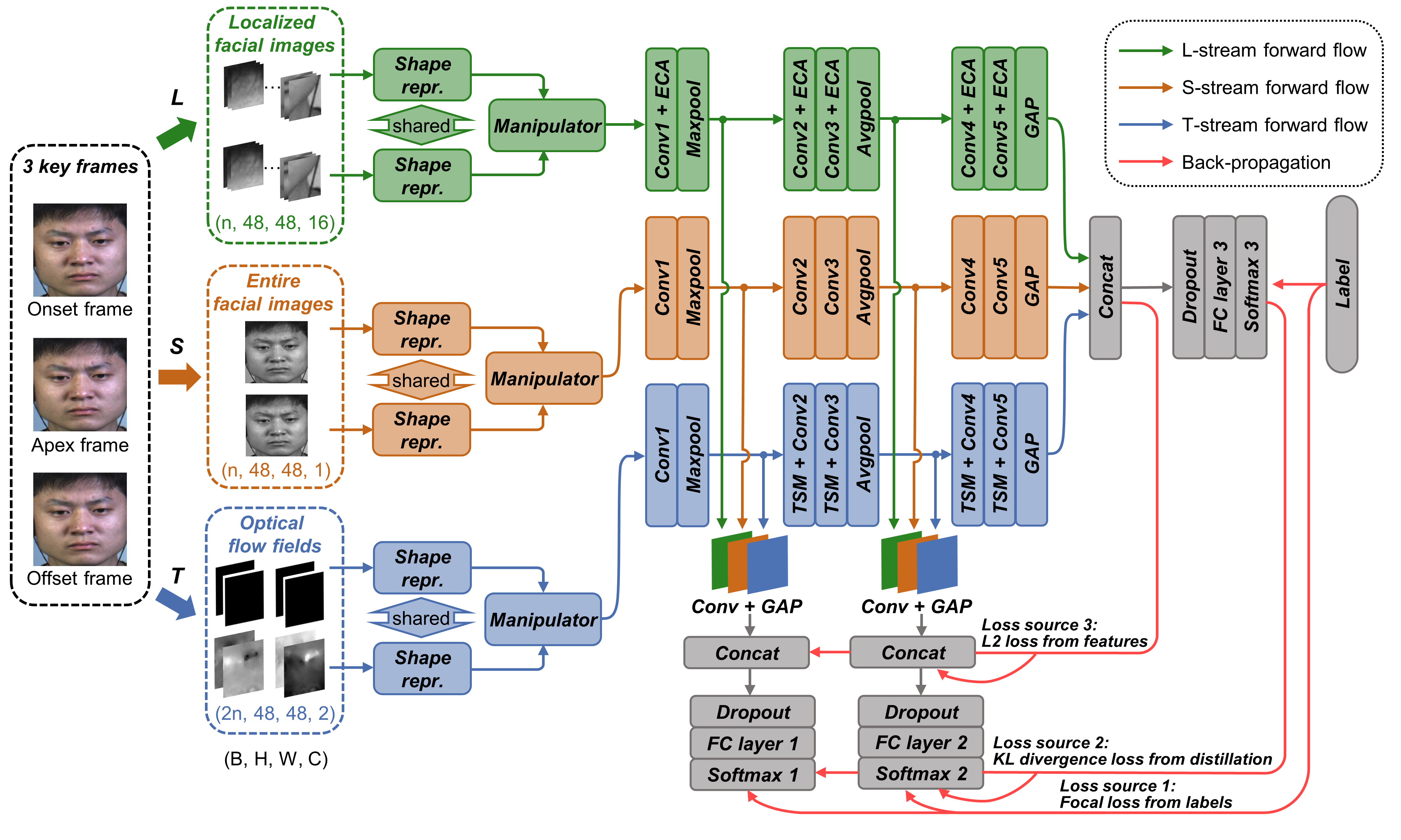
Figure 1: The overview of our SKD-TSTSAN framework, including three streams with different types of input data. Each stream contains a motion magnification module. The L-stream includes ECA modules, and the T-stream contains TSMs. Two auxiliary classifiers are added after the first and third convolutional layers for SKD.

two-stage distillation, designing an appropriate teacher model is challenging. Moreover, excellent student models that outperform teacher models are rare due to inefficient knowledge transfer [17].

To address the shortcomings of traditional distillation, we employ the self-distillation framework proposed in [17], which adds multiple auxiliary classifiers (AC) to the model. The deepest part and the shallow part with classifiers are respectively treated as the teacher model and the student model, achieving single-stage self-knowledge distillation (SKD). Experimental results show that using SKD improves network performance while maintaining low complexity.

3 Method

The framework of our SKD-STSTAN is illustrated in Fig. 1. Firstly, the onset and apex frames of ME sequences as well as the motionless and real optical flow images are fed into the motion magnification modules to obtain the amplified shape representation, which is discussed in detail in Section 3.1. Then, the magnified apex frame representation is input into the static-spatial stream (S-stream) to obtain the contour and appearance information of the whole face. The representation of the magnified local blocks is input into the local-spatial stream (L-stream) for the local ME feature extraction. The efficient channel attention (ECA) module [14] used in the L-stream is introduced in Section 3.2. The amplified optical flow maps are input into the dynamic-temporal stream (T-stream), and the temporal shift module (TSM) [15] used in the T-stream is introduced in Section 3.3. Finally, the outputs of three recognition streams are fused into a fully connected layer to get the classification results. Furthermore, we add multiple auxiliary classifiers (ACs) in the network, leveraging SKD to enable all blocks to fully learn the features of the training set, which is discussed in Section 3.4.

3.1 Motion Magnification Module

Due to the low intensity of ME, we enhance muscle movements based on transfer learning using the motion magnification network proposed by Oh et al. [13] To achieve an end-to-end framework and avoid noise in magnified images reconstructed in the decoder, our motion magnification module does not use a decoder. Given that each stream in our three-stream network has different inputs, we add separate motion magnification modules for each stream. Specifically, the input to the motion magnification network includes two frames with small motion displacement. For an ME sequence, the onset frame is the first frame where the ME begins, and the apex frame is the frame where the facial expression reaches maximum intensity, conveying significant emotional information. Therefore, the onset and apex frames are employed as inputs for the motion magnification module of the S-stream, and the concatenation of their $n\times n$ grid divisions as inputs for the L-stream’s motion magnification module. Particularly, since the T-stream extracts temporal information from optical flow fields, we utilize the optical flow corresponding to no motion and the optical flow between the onset and apex frames (or: between the apex and offset frames) as inputs for the motion magnification module in the T-stream.

Additionally, according to [24], shape representation often reflects boundaries with geometric properties, while texture representation usually represents color properties. Therefore, shape representation is more helpful for the network to learn the relationships of muscle movements, whereas texture representation provides little useful information for ME. Moreover, the manipulator in the motion magnification module works by calculating the difference between two shape representations and multiplying it by an amplification factor, without using the texture representation, as shown below:

$${{G}_{m}}({{M}_{a}},{{M}_{b}},\alpha)={{M}_{a}}+h(\alpha\cdot g({{M}_{b}}-{{M}_{a}})),$$ (1)

where ${{G}_{m}}(\cdot)$ denotes manipulator; ${{M}_{a}},{{M}_{b}}$ represents the shape representations of two input frames; $g(\cdot)$ is a $3\times 3$ convolution followed by ReLU; $\alpha$ denotes the amplification factor; $h(\cdot)$ represents a $3\times 3$ convolution followed by a $3\times 3$ residual block. Therefore, we remove the texture representation extraction part and keep only the shape representation extraction part, reducing the complexity of the motion magnification module.

After the motion magnification modules, the motion-amplified face and optical flow field shape representations are obtained in each stream, and then we will extract global spatial information, local-spatial information, and temporal information in the S-, L-, and T-streams, respectively.

3.2 Efficient Channel Attention Module

MEs only appear as subtle muscle movements in localized facial areas, such as the mouth and eyebrows. Therefore, the input to the L-stream, i.e., the $n\times n$ facial blocks, contains redundant information, which may affect emotion classification. However, we cannot simply select parts of the facial blocks, as different emotions correspond to distinct AUs involving various facial regions. For instance, AU6 (“Cheek Raiser”) mainly reflects happiness, whereas the ME for surprise does not involve this facial region. Thus, an adaptive approach should be used to extract important information from the $n\times n$ facial blocks while suppressing unimportant information.

Therefore, we employ efficient channel attention (ECA) modules [14] in the L-stream, introducing an efficient channel attention mechanism. Specifically, compared to the original squeeze-and-excitation (SE) block [35], the ECA module avoids disrupting the direct relationship between channels and their weights and uses 1D convolution to achieve local cross-channel interaction. As illustrated in Fig. 2, the input feature map is $X\in{{\mathbb{R}}^{W\times H\times C}}$, where $W,H,C$ represents the width, height, and channel dimensions. The original ECA module employs global average pooling (GAP) to aggregate global spatial features into ${{F}_{avg}}\in{{\mathbb{R}}^{1\times 1\times C}}$. Additionally, we employ global maximum pooling (GMP) to provide the most significant information for each channel, obtaining ${{F}_{max}}\in{{\mathbb{R}}^{1\times 1\times C}}$. Then, by performing a 1D convolution with a

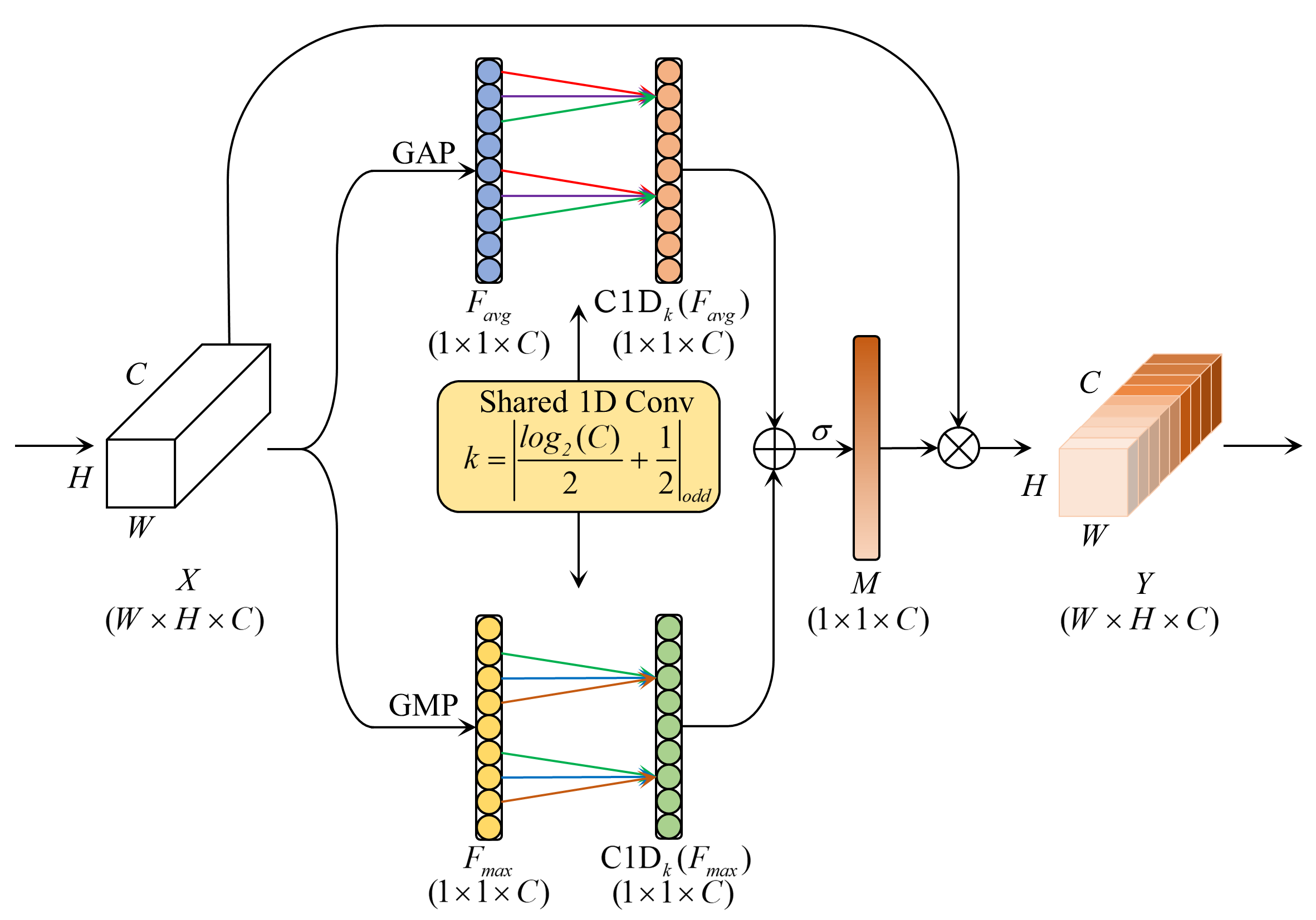
Figure 2: Diagram of our enhanced efficient channel attention (ECA) module.

kernel size of $k$ on ${F}_{avg}$ and ${F}_{max}$, we capture cross-channel interactions and obtain the channel weights $M\in{{\mathbb{R}}^{1\times 1\times C}}$, which are represented as follows:

$$M=\sigma(\text{C1}{{\text{D}}_{k}}({{F}_{avg}})+\text{C1}{{\text{D}}_{k}}({{F}_{max}})),$$ (2)

where $\text{C1}{{\text{D}}_{k}}$ denotes the 1D convolution with kernel size $k$, which is adaptively adjusted based on the number of channels:

$$k={{\left|\frac{lo{{g}_{2}}(C)}{2}+\frac{1}{2}\right|}_{odd}},$$ (3)

where ${{\left|t\right|}_{odd}}$ denotes the nearest odd value of $t$. Finally, the channel-wise refined output feature map is calculated as follows:

$$Y=M\otimes X,$$ (4)

where $\otimes$ represents element-wise multiplication.

We added the enhanced ECA module after each convolutional layer in the L-stream, using the channel attention mechanism to suppress the impact of redundant information on emotion classification.

3.3 Temporal Shift Module

3D CNNs can effectively mine spatiotemporal information but are computationally intensive. In order to extract spatiotemporal information while

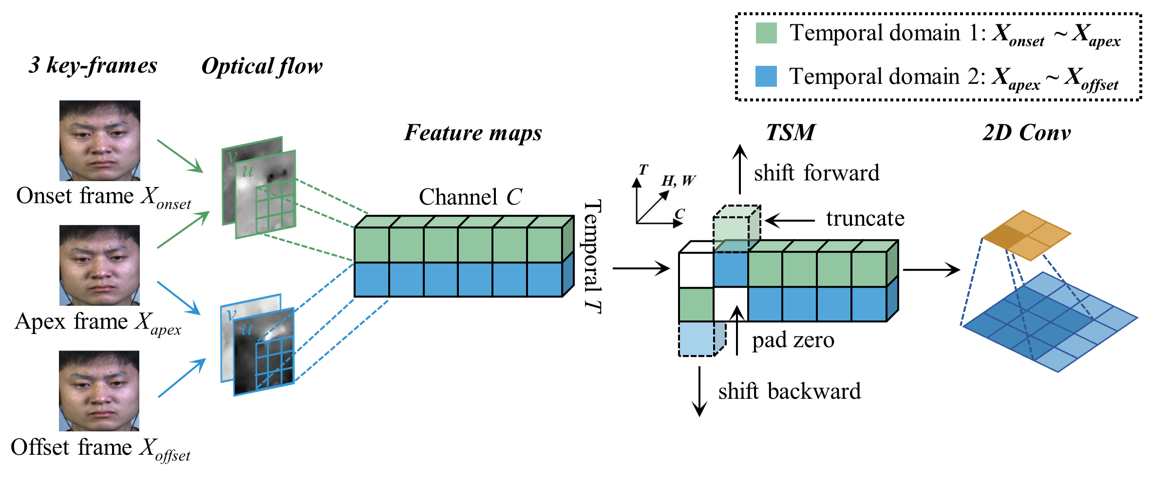
Figure 3: Illustration of the bi-directional TSM used in T-stream. The optical flow fields in two different temporal domains are calculated, where $u$ denotes the horizontal optical flow and $v$ represents the vertical optical flow. Temporal modeling is achieved by shifting channels along the temporal dimension. The subsequent 2D convolution performs the multiply-accumulate operation on the features from different frames’ channels.

keeping the complexity of 2D CNNs, we incorporate the temporal shift module (TSM) [15] into the T-stream.

The schematic of the TSM we use is shown in Fig. 3. Since the ME videos are offline videos, with access to future frames, the bi-directional TSM is employed. For a tensor with C channels and T frames, we use varying colors to represent features at different time stamps. By shifting part of the channels forward by one frame and another part backward by one frame along the temporal dimension, we achieve the mixing of information from past and future frames with the current frame. The excess channels are truncated and the blank frame parts are filled with zeros. The shift operation in TSM does not require any multiplication, and the multiply-accumulate operation of features from different frames’ channels is completed by the subsequent 2D convolution. Therefore, efficient temporal modeling is achieved at no extra cost.

As shown in Fig. 4(a), in the original TSCNN, the input to the T-stream is the concatenation of horizontal and vertical optical flows between the onset frame, apex frame, and offset frame pairs. It can be seen that 2D CNN without TSM have difficulty in capturing temporal relationships in forward propagation. To introduce TSM, we separate the inputs of the T-stream along the temporal dimension, i.e., the optical flow maps between the onset frame and the apex frame and between the apex frame and the offset

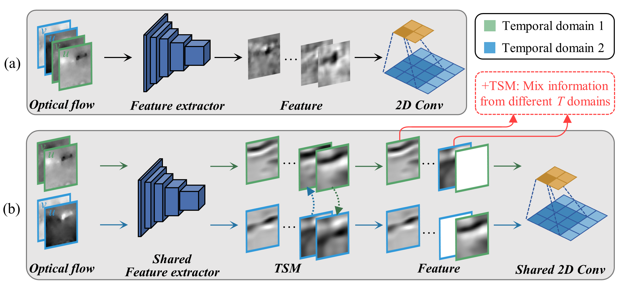
Figure 4: The forward propagation of the T-stream in the network. (a) and (b) represent the forward propagation of the T-stream in the network without and with TSM, respectively. Different border colors indicate that the information comes from different temporal domains.

frame, containing motion information from two different temporal domains. As illustrated in Fig. 4(b), TSMs are added before all convolutional layers in the intermediate layers of the T-stream to mix information from the two different temporal domains, enhancing the model’s temporal modeling capability. When the ratio of shifted channels in TSM is too big, it may affect the learning of spatial features; if too small, the temporal modeling capability is insufficient to handle complex temporal relationships. [15] Therefore, we shift 1/8 of the channels in the TSM.

3.4 Self-Knowledge Distillation

In order to further improve our lightweight three-stream network’s performance, we introduce an effective model compression strategy, self-knowledge distillation (SKD) [17]. In traditional knowledge distillation, a complex teacher model is first trained, and then a compact student model imitates the predictions of the teacher model [33]. However, it is difficult to design an effective over-parameterized model to act as the teacher model on a small-scale ME dataset [17]. Instead, in SKD, the model acts as its own teacher, using knowledge acquired from the training set to guide its own training. This approach requires less training time than the two-stage method and achieves better results.

We adopt the Be Your Own Teacher (BYOT) framework proposed by Zhang et al. [17], adding two auxiliary classifiers (ACs) after the first and third convolutional layers of the network. Each AC has a three-stream architecture similar to the main network, including convolutional layers and a fully connected layer, and contains the previously mentioned ECA modules and TSMs. The ACs are only used during training and can be removed during inference. During the training stage, the deepest part of the network acts as the teacher model, while the shallow parts with the corresponding classifiers serve as the student model. We employ three kinds of loss functions: focal loss (FL) [36], Kullback-Leibler (KL) divergence loss, and L2 loss. Then the computation methods for each loss function will be detailed.

Given a training set $D$ for a MER task, we use $\{x,y\}\in D$ to represent each sample in the dataset, where $x$ denotes the input and $y$ denotes the label. Suppose there are $K$ classes, so $y\in\{1,\ldots,K\}$. The multiple classifiers in the network are represented as $\Theta=\{{{\theta}_{i}}\}_{i=1}^{C}$, where $C$ indicates the number of classifiers, and ${{\theta}_{C}}$ represents the deepest classifier. We use ${{z}^{c}}$ to denote the output following the fully connected layer of classifier ${{\theta}_{c}}$, and $z_{i}^{c}$ to denote the logit corresponding to the ${{i}_{th}}$ class in the output ${{z}^{c}}$. Each classifier is followed by a softmax layer:

$$q_{i}^{c}(T)=\frac{\exp(z_{i}^{c}/T)}{\sum\limits_{j=1}^{K}{\exp(z_{j}^{c}/T)}},$$ (5)

where $q_{i}^{c}$ indicates the class probability of the class ${{i}_{th}}$ for the classifier ${{\theta}_{c}}$. $T$ denotes the distillation temperature, where a large $T$ is used to soften the class probability distribution.

All classifiers are supervised by the labels. To address data imbalance and focus more on hard examples, we choose focal loss to implement the supervision from labels. We first define ${t_{i}}$ to represent the true probability distribution as follows:

$${{t}_{i}}=\left\{\begin{array}[]{*{35}{l}}1,&i=true\ label\\ 0,&i\neq true\ label\\ \end{array}\right..$$ (6)

The multi-class focal loss we use is defined as follows:

$$L_{FL}^{i}({{q}^{i}}(T),y)=-\sum\limits_{k=1}^{K}{{{\alpha}_{k}}{{(1-q_{k}^{i}(T))}^{\gamma}}{{t}_{k}}\log(q_{k}^{i}(T))},$$ (7)

where ${{q}^{i}}$ denotes the output probability of the classifier ${{\theta}_{i}}$. The focusing parameter $\gamma$ determines the rate at which the weights of easy samples are reduced, and ${{\alpha}_{k}}$ represents the weighting factor for the class ${{k}_{th}}$. ${{\alpha}_{k}}$ is used to address class imbalance, generally set utilizing the inverse class frequency.

The supervision for the deepest classifier ${{\theta}_{C}}$ comes only from ${{L}_{FL}}$, while the supervision for the auxiliary classifiers also comes from the KL divergence loss ${{L}_{KL}}$ and the L2 loss ${{L}_{L2}}$. ${{L}_{KL}}$ is calculated between ${{q}^{i}}$ and the probability output ${{q}^{C}}$ of the deepest classifier, reflecting the supervision from distillation. ${{L}_{KL}}$ is represented as follows:

$$L_{KL}^{i}({{q}^{i}}(T),{{q}^{C}}(T))={{T}^{2}}\sum\limits_{k=1}^{K}{q_{k}^{C}(T)\log\frac{q_{k}^{C}(T)}{q_{k}^{i}(T)}}.$$ (8)

The purpose of ${{L}_{L2}}$ is to use the output of hidden layers of the deepest classifier to guide the learning of the shallow classifiers, aiming to reduce the distance between their feature maps. Since feature maps at different depths have different sizes, convolutional layers are employed in ACs to align them. ${{L}_{L2}}$ is defined as follows:

$$L_{L2}^{i}=\left\|{{F}_{i}}-{{F}_{C}}\right\|_{2}^{2},$$ (9)

where ${{F}_{i}}$ and ${{F}_{C}}$ represent the features of the classifier ${{\theta}_{i}}$ and the deepest classifier ${{\theta}_{C}}$, respectively.

In summary, the total loss function of the proposed SKD-TSTSAN is expressed as:

$$L=\sum\limits_{i=1}^{C}{[(1-{{\lambda}_{1}})L_{FL}^{i}({{q}^{i}}(1),y)+{{\lambda}_{1}}\cdot L_{KL}^{i}({{q}^{i}}(T),{{q}^{C}}(T))+{{\lambda}_{2}}\cdot L_{L2}^{i}]},$$ (10)

where ${{\lambda}_{1}}$ and ${{\lambda}_{2}}$ are hyperparameters used to balance the loss terms. For the deepest classifier, both ${{\lambda}_{1}}$ and ${{\lambda}_{2}}$ are set to 0, indicating that its supervision comes only from the labels.

4 Experiments

In this section, we will provide the details of our experiments, including the datasets used, data pre-processing, implementation details, and evaluation metrics. Additionally, the results and analysis of the comparative experiments with other SOTA methods, ablation studies, and parameter setting experiments will be provided.

4.1 Datasets

We evaluate our SKD-TSTSAN on four spontaneous ME datasets: the CASME II [7], SAMM [8], MMEW [9], and CAS(ME)³ [10] databases. The details of these datasets are introduced below.

1. The CASME II dataset includes 255 ME samples from 26 participants, which are recorded at 200 fps with a facial resolution of $280\times 340$. These samples are divided into seven categories: Happiness (32), Disgust (63), Repression (27), Surprise (25), Sadness (7), Fear (2), and Others (99), where the numbers in brackets represent the number of corresponding MEs. Due to the small number of samples in the “Sadness” and “Fear” categories, each having fewer than 10 samples, the CASME II dataset is usually used to study a 5-category MER task involving the remaining 5 categories. Additionally, some studies classify emotion categories into 3 categories: the “Positive” emotion category contains “Happiness” class, the “Negative” category contains “repression” and “disgust” classes, and the “Surprise” category includes only the “Surprise” class. Our experiments include both 3- and 5-category tasks on the CASME II dataset.

2. The SAMM dataset includes 159 ME samples from 29 participants, recorded at a frame rate of 200 fps and a facial resolution of $400\times 400$. Eight emotion categories are labeled in SAMM: Anger (57), Happiness (26), Surprise (15), Contempt (12), Disgust (9), Fear (8), Sadness (6), and Others (26). In our experiments, we considered the 3-category task. The 3-category task includes a “Positive” category that includes “Happiness” class, a “Negative” category that includes “Anger”, “Disgust”, “Contempt”, “Sadness”, “Fear” classes, and a “Surprise” category that included only “Surprise” class.

3. The MMEW dataset includes 300 ME samples and 900 macro-expression samples from 36 participants. They are recorded using a frame rate of 90 fps with a facial resolution of $400\times 400$. The ME samples are divided into seven categories: Happiness (36), Disgust (72), Surprise (89), Fear (16), Sadness (13), Anger (8) and Others (66). In our experiments, we use four and six emotion categories respectively. For the 6-class MER task on the MMEW dataset, the “Anger” category is excluded. When performing the 4-class MER task, we select four categories that are close in number: Happiness, Disgust, Surprise, and Others.

4. The CAS(ME)³ dataset is a large-scale spontaneous ME dataset, which provides about 80 hours of video at a frame rate of 30 fps and offers depth information as an additional modality. According to the latest version of the dataset annotations, there are 860 manually labeled MEs, divided into seven categories: Anger (64), Disgust (250), Fear (86), Happy (55), Others (161), Sad (57), and Surprise (187). In our experiments, classification tasks are conducted with 3,4, and 7 emotion categories. For the 3-category classification, we group negative emotions (“Anger”, “Disgust”, “Fear”, and “Sad”) into a “Negative” category, “Happy” into a “Positive” category, and “Surprise” into the third category. In the 4-category classification, we add the “Others” category. The 7-category classification uses all the official emotion categories.

4.2 Data Pre-Processing and Implementation Details

As the proposed SKD-TSTSAN requires knowledge transfer from macro-expression data, we first pre-train it on the CK+ dataset [16], which includes seven expressions: Happiness, Anger, Disgust, Contempt, Fear, Sadness, and Surprise. The CK+ dataset, being a macro-expression dataset, lacks annotations like the apex frames present in ME datasets. Therefore, to pre-train the network using this dataset, we designate the last frame with the most obvious muscle movement of each sample as the apex frame, and the first frame as both the onset and offset frames.

For each input sample, Retinaface [37] is first employed to detect the facial region and resize it to $128\times 128$. Then, we compute optical flow features using the TV-L1 method [38]. The entire facial region is scaled down to $48\times 48$ and fed into the S-stream of our network. The $128\times 128$ facial region is divided into a $4\times 4$ grid, resulting in 16 patches, each scaled to $48\times 48$. These patches are concatenated along the channel dimension and fed into the L-stream. Finally, the horizontal and vertical optical flow fields between the three key-frames are combined into two $48\times 48$ 2-channel images, which are fed into the T-stream of the network.

We implement our SKD-TSTSAN model on an NVIDIA-RTX-4090 GPU. The Adam optimizer is utilized with learning rate, betas and weight decay set to 1e-3, (0.9, 0.99) , 5e-4, respectively. Loss weights ${{\lambda}_{1}}=0.1$, ${{\lambda}_{2}}=1e-6$ and distillation temperature $T=3$ are chosen as default values. In the multi-class focal loss, the focusing parameter $\gamma$ is set to 2, and the weighting factor ${{\alpha}_{k}}$ is positively correlated with the inverse of the sample size for each category. In our motion magnification module, we set the amplification factor to 2. During the pre-training stage on the CK+ dataset, we configure the training iterations to 10k and the batch size to 16. When training on the CASME II, SAMM, and MMEW datasets with smaller data volumes, the batch size is set to 16, while for the CAS(ME)³ dataset, it is set to 32. Training iterations on the ME dataset are set to 20k and early stopping is used to alleviate overfitting.

4.3 Evaluation Metrics

For all experiments on the four public datasets, we employ leave-one-subject-out (LOSO) cross-validation. The unweighted accuracy (UAR) and unweighted F1 score (UF1) are used to evaluate the MER results. For convenience, $T{{P}_{i}}$, $F{{P}_{i}}$, and $F{{N}_{i}}$ are used to represent the predicted numbers of true positives, false positives, and false negatives for each class. $UF1$ and $UAR$ are calculated as follows:

$$UF1=\frac{1}{C}\sum\limits_{i=1}^{C}{\frac{2\times T{{P}_{i}}}{T{{P}_{i}}+F{{P}_{i}}+F{{N}_{i}}}},$$ (11)

$$UAR=\frac{1}{C}\sum\limits_{i=1}^{C}{\frac{T{{P}_{i}}}{{{N}_{i}}}},$$ (12)

where $C$ represents the number of emotion categories in the dataset, and ${{N}_{i}}$ denotes the total number of MEs in the class ${{i}_{th}}$.

4.4 Comparative Experiments Results

In this section, we compare the results of our method with other SOTA methods using four public ME datasets (CASME II, SAMM, MMEW, and CAS(ME)³). As seen in Tables 2 to 4, our SKD-TSTSAN demonstrates significant performance improvements in the MER task. Furthermore, the confusion matrices of our SKD-TSTSAN on different datasets are shown in Fig. 5.

As shown in Table 2, we report the performance of SKD-TSTSAN on the CASME II dataset and compare it with other methods. Our SKD-TSTSAN achieves optimal performance on both 3-category and 5-category MER tasks. When performing the 3-category classification, SKD-TSTSAN achieves a superior 99.13% UF1 score and 98.67% UAR, exhibiting a 3.81% UF1 improvement and 3.51% UAR improvement compared to the second-ranked MER method, HTNet [23]. For the 5-category emotion classification, SKD-TSTSAN achieved the highest UF1 of 90.34% and UAR of 89.47%,

Table 1: Comparisons with other approaches on CASME II dataset.

Method	# Classes	UF1 (%)	UAR (%)
LR-GACNN [39]	5	70.90	81.30
AMAN [26]	5	71.00	75.40
Graph-TCN [24]	5	72.46	73.98
MiMaNet [12]	5	75.90	79.90
SMA-STN [40]	5	79.46	82.59
TSCNN [11]	5	80.70	80.97
$\mu$-BERT [41]	5	85.53	83.48
SKD-TSTSAN (ours)	5	90.34	89.47
STSTNet [42]	3	83.82	86.86
OFF-ApexNet [43]	3	86.97	88.28
$\mu$-BERT [41]	3	90.34	89.14
HTNet [23]	3	95.32	95.16
SKD-TSTSAN (ours)	3	99.13	98.67

Table 2: Comparisons with other approaches on SAMM dataset.

Method	# Classes	UF1 (%)	UAR (%)
OFF-ApexNet [43]	3	54.09	53.92
STSTNet [42]	3	65.88	68.10
EMR [44]	3	77.54	71.52
FeatRef [45]	3	73.72	71.55
HTNet [23]	3	81.31	81.24
SKD-TSTSAN (ours)	3	94.29	92.65

compared to $\mu$-BERT’s 85.53% UF1 and 83.48% UAR. Furthermore, compared to our baseline TSCNN, SKD-TSTSAN shows a 9.64% UF1 and 8.50% UAR improvement, proving the effectiveness of our submodules.

Table 2 presents the quantitative comparison results for the 3-category MER task on the SAMM dataset. Our SKD-TSTSAN achieves a UF1 of 94.29% and a UAR of 92.65%, showing an increase of 12.98% and 11.41% compared to the previous leading method HTNet [23]. All these methods are deep learning approaches that utilize optical flow features. The difference is that our SKD-TSTSAN uses the optical flow fields between the three key-frames as the input to the T-stream, while the other methods [42, 23, 43, 44, 45] only utilize the optical flow field between the onset frame and the apex frame. Therefore, SKD-TSTSAN can leverage motion information from different temporal regions for temporal modeling, fully considering the temporal information of ME and achieving the best recognition performance.

The performance of SKD-TSTSAN on the MMEW dataset is compared

Table 3: Comparisons with other approaches on MMEW dataset.

Method	# Classes	UF1 (%)	UAR (%)
CapsuleNet [46]	6	44.13	45.31
MMNet [47]	6	57.05	56.95
STSTNet [42]	6	64.13	62.65
TSCNN [11]	6	70.43	68.76
SKD-TSTSAN (ours)	6	77.11	74.77
CapsuleNet [46]	4	64.02	63.15
STSTNet [42]	4	78.99	78.89
TSCNN [11]	4	86.46	86.09
MMNet [47]	4	86.35	87.45
SKD-TSTSAN (ours)	4	90.41	90.44

Table 4: Comparisons with other approaches on CAS(ME)³ dataset.

Method	# Classes	UF1 (%)	UAR (%)
FR [45]	3	34.93	34.13
STSTNet [42]	3	37.95	37.92
RCN-A [48]	3	39.28	38.93
$\mu$-BERT [41]	3	56.04	61.25
SKD-TSTSAN (ours)	3	86.48	83.44
AlexNet [10]	4	29.15	29.10
AlexNet(+Depth) [10]	4	30.01	29.82
SFAMNet [49]	4	44.62	47.97
$\mu$-BERT [41]	4	47.18	49.13
SKD-TSTSAN (ours)	4	76.40	72.57
AlexNet [10]	7	17.59	18.01
AlexNet(+Depth) [10]	7	17.73	18.29
SFAMNet [49]	7	23.65	23.73
$\mu$-BERT [41]	7	32.64	32.54
SKD-TSTSAN (ours)	7	59.95	57.31

with different methods in Table 4. We conduct experiments on the MMEW dataset using CapsuleNet [46], MMNet [47], STSTNet [42], and TSCNN [11]. For MMNet’s performance on the 4-category MER task, the optimal performance reported in their original paper is provided. For six categories, CapsuleNet obtains the lowest UF1 and UAR since it only uses the apex frame as the network input, which makes it difficult to extract the motion and temporal information of MEs. In contrast, STSTNet and TSCNN use the optical flow as input and achieve better performance. Our SKD-TSTSAN achieves the best recognition performance, reaching 77.11% UF1 and 74.77% UAR and showing improvements of 6.68% and 6.01% over TSCNN. Similar

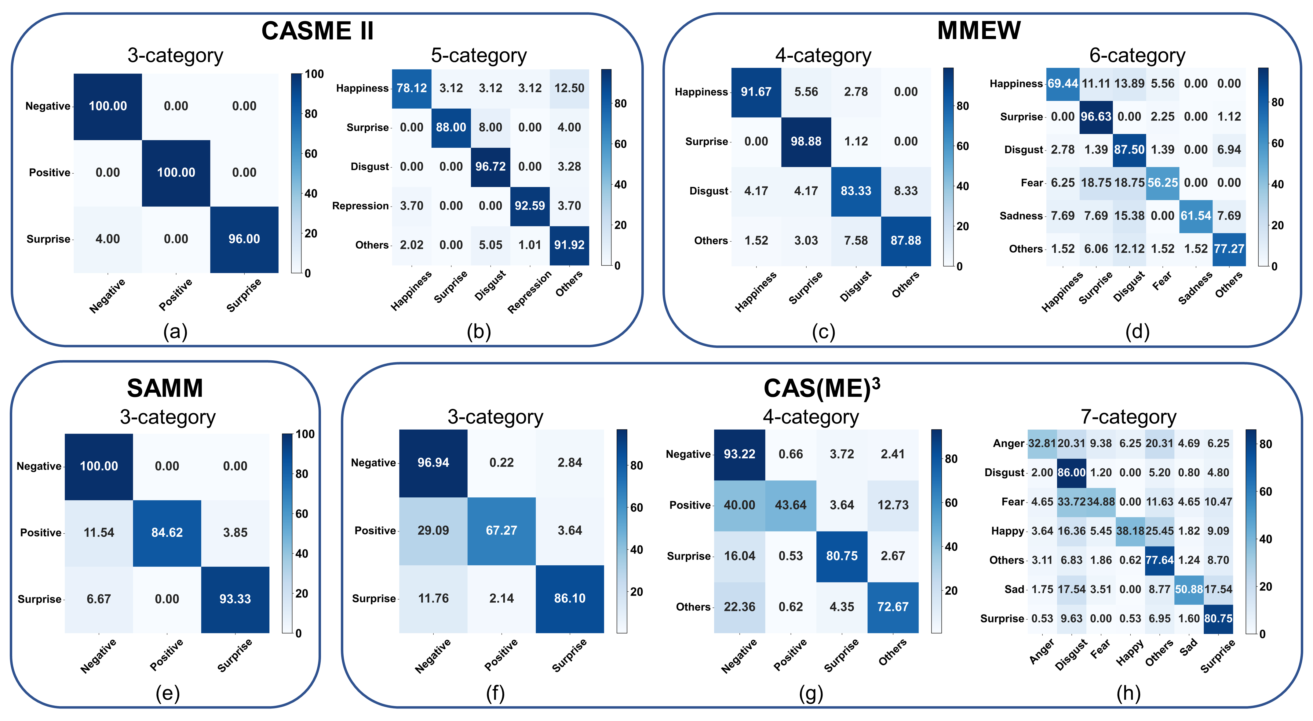
Figure 5: Confusion matrices for MER with SKD-TSTSAN on CASME II, SAMM, MMEW, and CAS(ME)³ datasets. (a) and (b) denote the 3-class and 5-class classification results on CASME II. (c) and (d) indicate the results of 4-class and 6-class classification on MMEW. (e) shows the results of 3-class classification on SAMM. (f), (g), and (h) represent the 3-class, 4-class, and 7-class classification results on CAS(ME)³, respectively.

improvements are observed in the 4-category emotion classification: a 3.95% over TSCNN for UF1 and a 2.99% increase over MMNet for UAR.

To further validate our proposed SKD-TSTSAN, we perform comparative experiments on the large-scale ME dataset CAS(ME)³ using 3, 4, and 7 emotion categories, as shown in Table 4. When tested with 3, 4, and 7 emotion categories, SKD-TSTSAN exhibits double-digit improvements over all other methods. In the case of 3 emotion categories, SKD-TSTSAN obtains a UF1 score of 86.48% and a UAR score of 83.44%, which indicates an improvement of 30.44% in UF1 and 22.19% in UAR compared to the second-ranked $\mu$-BERT [41]. For the 4 emotion categories, our SKD-TSTSAN maintains a considerable advantage over other methods with over 29.22% in UF1 and 23.44% in UAR. Using all 7 emotion categories is more demanding on the recognition performance of the MER method. SKD-TSTSAN significantly outperforms $\mu$-BERT in terms of UF1 (59.95% vs 32.64%) and UAR (57.31% vs 32.54%).

In addition, the confusion matrices in Fig. 5 report the results of SKD-TSTSAN on multiple datasets. We can see that on the CASME II and SAMM

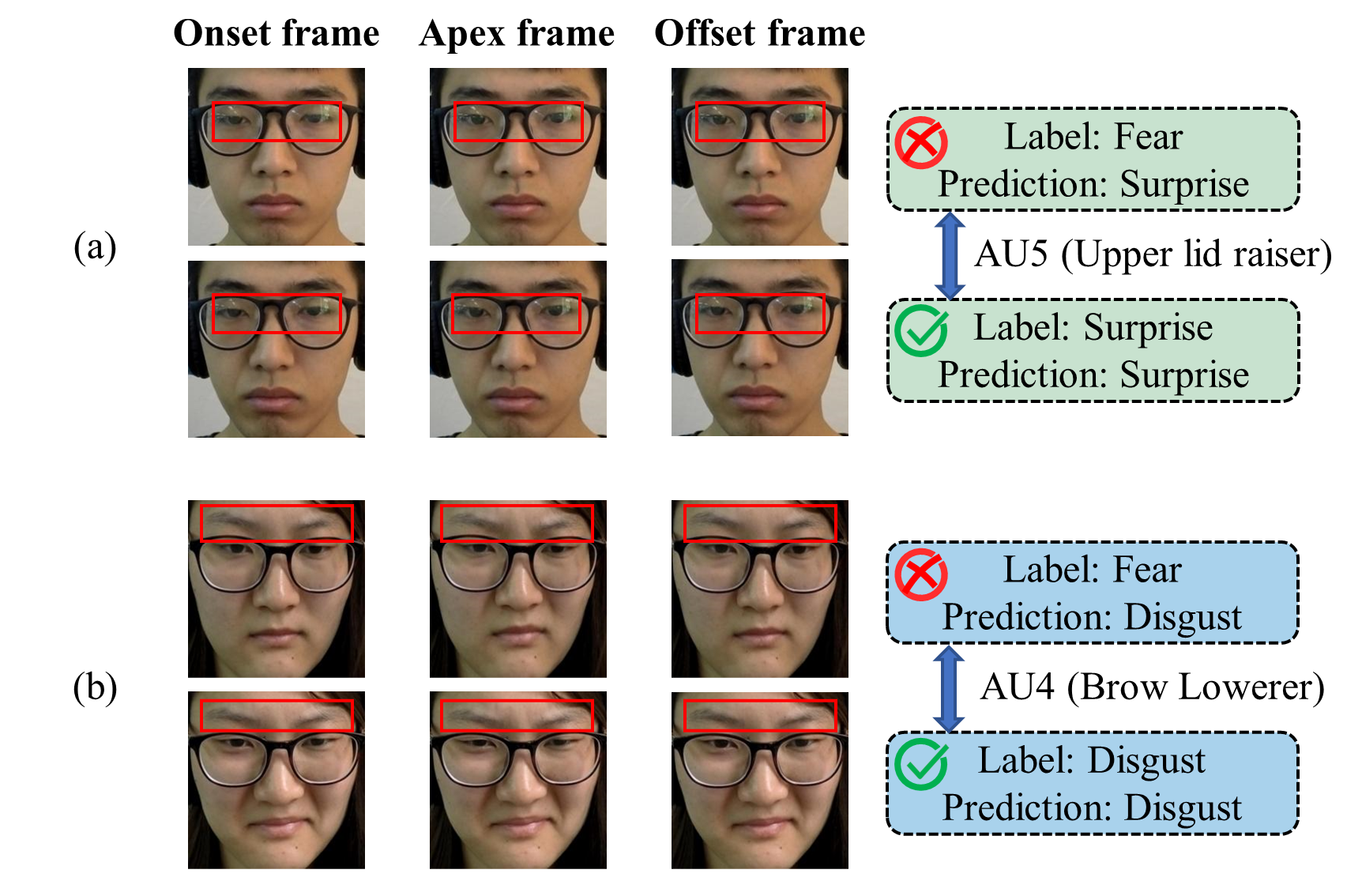
Figure 6: Some correctly and incorrectly classified samples in the 6-class classification on the MMEW dataset. (a) indicates that a sample labeled as “Fear” is predicted as “Surprise”. Both it and another correctly classified sample labeled as “Surprise” appear in AU5. (b) shows a sample labeled as “Fear” is predicted as “Disgust”. Similar to another sample labeled as “Disgust”, it occurs in AU4.

datasets, SKD-TSTSAN achieves good recognition results for all categories. On the MMEW dataset, SKD-TSTSAN performs well on the 4-class MER task. On the 6-class MER task, SKD-TSTSAN has poor recognition performance for the “Fear” and “Sadness” samples. One of the main reasons is the small number of samples for the “Fear” and “Sadness” emotion categories. Besides, different emotion categories may correspond to the same AU. For example, both “Fear” and “Surprise” expressions appear in AU5 (“Upper Lid Raiser”), while “Fear” and “Disgust” expressions both involve AU4 (“Brow Lowerer”), as shown in Fig. 6. Therefore, samples labeled as “Fear” are easily misclassified as “Surprise” and “Disgust” categories, which have larger sample sizes. On the CAS(ME)³ dataset, the performance of SKD-TSTSAN is also affected by the imbalanced class distribution. For the 3 and 4 emotion categories, SKD-TSTSAN has poorer recognition performance on “Positive”, which has fewer samples. For the 7 emotion categories, SKD-TSTSAN performs better in the “Disgust”, “Others”, and “Surprise” categories. One of the reasons for the poor performance on the CAS(ME)³ dataset is that the onset frame annotations of some samples are the same as the apex frame annotations. This results in no motion information in the optical flow between them, leading to misclassification.

Table 5: Ablation studies on the CASME II and MMEW datasets.

Methods				CASME II (5-category)		MMEW (6-category)
Mag	ECA	TSM	SKD	UF1 (%)	UAR (%)	UF1 (%)	UAR (%)
				77.49	75.85	66.42	64.23
✓				87.24	87.64	67.99	65.08
✓	✓			88.37	87.76	70.47	68.97
✓		✓		88.78	88.85	69.54	68.90
✓	✓	✓		88.80	89.10	73.78	71.31
✓	✓	✓	✓	90.34	89.47	77.11	74.77

4.5 Analysis and Discussion

4.5.1 Ablation Studies

In this section, to illustrate the effect of each component, we conduct ablation studies on the CASME II and MMEW datasets. Initially, a three-stream baseline network is trained using the focal loss ${{L}_{FL}}$. Subsequently, we incrementally introduce submodules into the baseline model, including motion magnification (Mag) modules, efficient channel attention (ECA) modules, temporal shift modules (TSMs), and self-knowledge distillation (SKD).

As presented in Table 5, compared to the baseline model, the introduction of motion magnification modules improves the UF1 and UAR of the 5-class MER task on the CASME II dataset by 9.75% and 11.79%. It also increases the UF1 and UAR of the 6-class MER task on the MMEW dataset by 1.57% and 0.85%, respectively. This indicates that motion magnification modules can improve MER performance by enhancing the motion intensity in each stream.

We introduce a channel attention mechanism by incorporating ECA modules into the L-stream of the network, which improves UF1 and UAR by 1.13% and 0.12% on the CASME II dataset, and 2.48% and 3.89% on the MMEW dataset. Furthermore, to better understand how ECA modules influence the final recognition performance, the gradient-weighted class activation mapping (Grad-CAM) [50] is utilized for visualization analysis. Fig. 7(a), (b), and (c) represent the samples of three different emotion categories in the CASME II dataset: “Negative (Disgust)”, “Positive (Happiness)”, and “Surprise”. The apex frames are shown in the first row, and the class activation maps (CAMs) of the SKD-TSTSAN with and without the ECA module are shown in the second and third rows. These maps are from the fourth convolutional layer of the S-stream, and the red regions highlight the areas that are crucial for the MER results. According to the Facial Action Coding

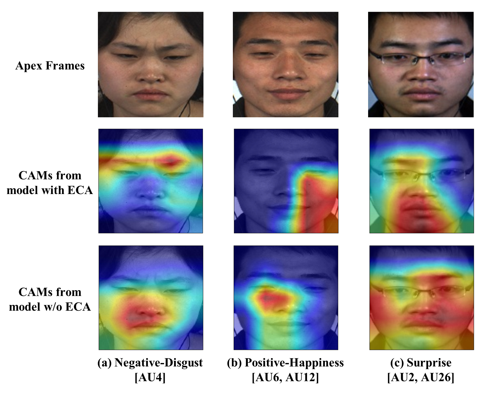
Figure 7: Visualization of class activation maps (CAMs) of three ME samples from the CASME II dataset. The first to third rows represent the apex frames, and CAMs from networks with and without ECA modules, respectively. The emotion label for (a) is “Negative (Disgust)”, reflected in AU4 (“Brow Lowerer”). The emotion label for (b) is “Positive (Happiness)”, appearing in AU6 (“Cheek Raiser”) and AU12 (“Lip Corner Puller”). The emotion label for (c) is “Surprise”, reflected in AU2 (“Outer Brow Raiser”) and AU26 (“Jaw Drop”).

System (FACS), the “Disgust” expression usually involves AU9 (“Nose Wrinkler”), AU10 (“Upper Lip Raiser”), and AU4 (“Brow Lowerer”) with AU7 (“Lid Tightener”). The “Happiness” expression often involves AU6 (“Cheek Raiser”) and AU12 (“Lip Corner Puller”). The “Surprise” expression is usually found in AU5 (“Upper Lid Raiser”), AU26 (“Jaw Drop”), AU1 (“Inner Brow Raiser”), and AU2 (“Outer Brow Raiser”). As seen in the CAMs in Fig. 7(a), (b), and (c), when ECA modules are used, the facial regions with strong activation are consistent with the AUs defined by FACS. For instance, in Fig. 7(a), the eyebrow region is highlighted; in Fig. 7(b), the cheek and lip corner regions are emphasized; in Fig. 7(c), the eyebrow and chin regions are highlighted. However, when the ECA module is not used, the model tends to focus on regions less relevant to the expressions. For example, the model without ECA modules focuses on the cheek area in Fig. 7(c), which is not relevant to the “Surprise” expression. Therefore, by incorporating ECA modules into the L-stream, we not only suppress redundant information in the L-stream input but also enable the S-stream to focus more on the key

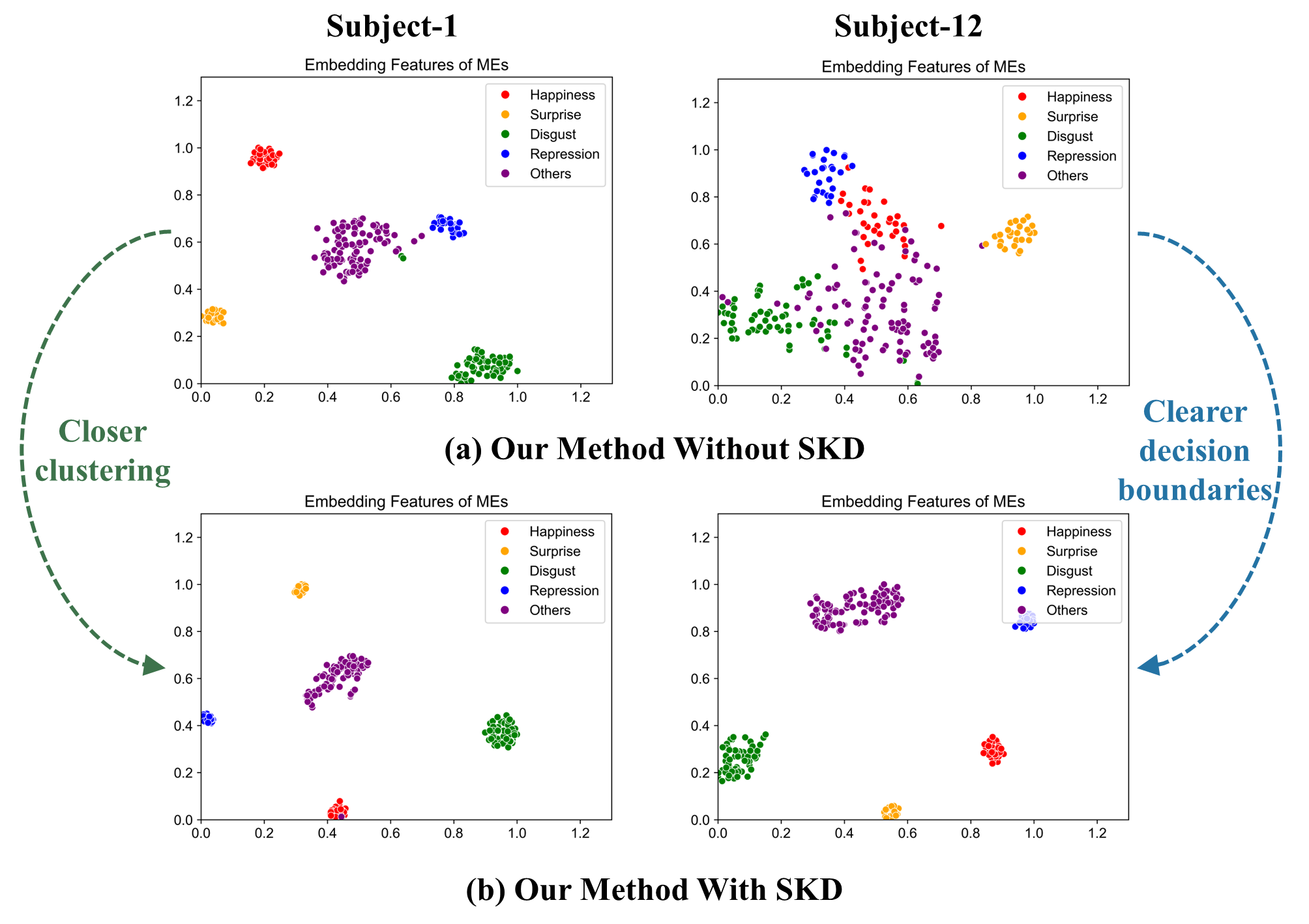
Figure 8: The t-SNE visualization of ME features generated by: (a) Our method without SKD; (b) SKD-TSTSAN.

regions of ME muscle movements.

Next, the introduction of TSM in the T-stream enables the exchange of temporal information between adjacent frames and also improves the performance on CASME II and MMEW datasets. When both ECA modules and TSMs are used, the performance is better than using only one of them, demonstrating the complementarity of the introduced modules. Furthermore, when the self-knowledge distillation (SKD) is introduced into MER, UF1 and UAR on CASME II are improved by 1.54% and 0.37%, and UF1 and UAR on MMEW are increased by 3.33% and 3.46%, respectively. For an intuitive analysis of the effect of SKD, as shown in Fig. 8, t-distributed stochastic neighbor embedding (t-SNE) is employed to visualize the learned ME features of subjects 1 and 12 in the CASME II dataset. Fig. 8(a) and (b) illustrate the embedding ME features of the network without and with SKD, respectively. It can be easily observed that with the addition of SKD, the clustering within the same category is closer, and the decision boundaries between different categories are clearer, thus the network has better performance. In addition, the deepest section of the network serves as the teacher model in SKD without the need to design and train an additional teacher model, which reduces the training time.

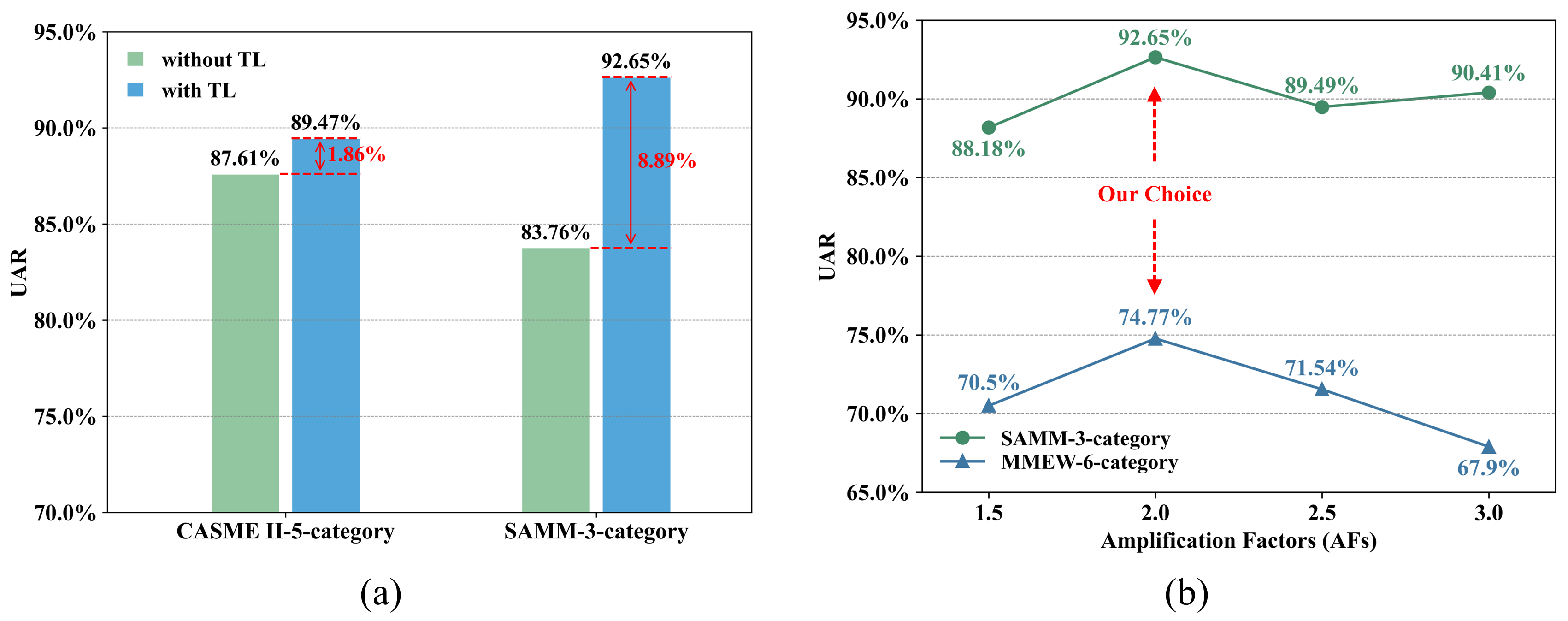
Figure 9: UAR performance of SKD-TSTSAN under different experimental configurations. (a) Comparison results with and without transfer learning on the CASME II and SAMM datasets. (b) Comparison results with different amplification factors on the SAMM and MMEW datasets.

4.5.2 More Analysis on the Effect of Transfer Learning

In Fig. 9(a), we provide the MER results on the CASME II and SAMM datasets without and with transfer learning (TL). The two sets of histograms indicate that the introduction of transfer learning effectively improves the MER performance by 1.86% for the UAR of the 5-class MER task on CASME II and 8.89% for the 3-class MER task on SAMM. This is due to the fact that macro-expressions have similar AUs to MEs in expressing emotions. Therefore, we employ transfer learning in all comparative experiments on ME datasets.

4.5.3 More Analysis on the Choice of Amplification Factors

To evaluate the effect of different amplification factors (AFs) on the performance, we provide the UAR under different AF configurations on the SAMM and MMEW datasets in Fig. 9(b). For the 3-class MER task on the SAMM dataset, our SKD-TSTSAN consistently outperforms the others MER methods ($\leq$81.24% UAR) regardless of the AF value, indicating the robustness and effectiveness of our approach. When the AF is too small, the facial muscle movements are not obvious; while when the AF is too large, the muscle movements are excessively deformed, both of which affect the MER performance. When the AF is set to 2, the results are optimal on both the SAMM and MMEW datasets, so this value is used as our final configuration.

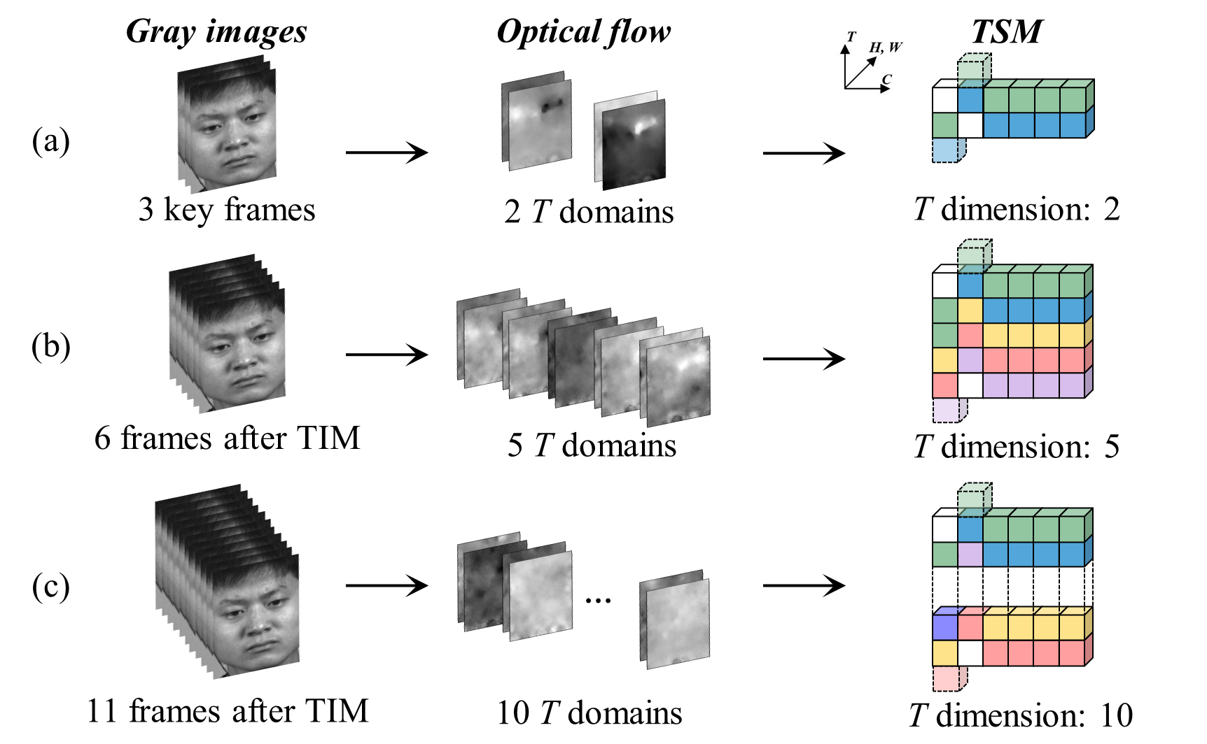
Figure 10: Visualization of T-flow inputs with different temporal domain distributions.

Table 6: Studies on T-stream input with different temporal domain distributions on the CASME II dataset with five emotion categories.

Number of Temporal domains	Metrics
	UF1 (%)	UAR (%)
2	90.34	89.47
5	86.10	86.22
10	87.38	86.67

4.5.4 More Analysis on the Temporal Domain Distribution

As illustrated in Fig. 10(a), in our comparative experiment configuration, our T-stream inputs are optical flow maps from two different temporal domains, calculated from the onset frame, apex frame, and offset frame. To explore the effect of different temporal distributions of T-stream inputs, as shown in Fig. 10(b) and (c), we first interpolate each ME sequence to 6 and 11 frames using the temporal interpolation model (TIM) [5]. The optical flow maps are then calculated between adjacent frames, representing the motion information from 5 and 10 different temporal domains, respectively. Subsequently, the optical flow maps from different temporal domains are input into the T-stream, where temporal modeling is performed using TSM. Table 6 provides the performance of our SKD-TSTSAN on the CASME II dataset under different temporal domain distributions. It’s clear that the optimal results are obtained when we use the optical flow between the three key-frames as T-stream input, with an improvement of 2.96% for UF1 and 2.80%

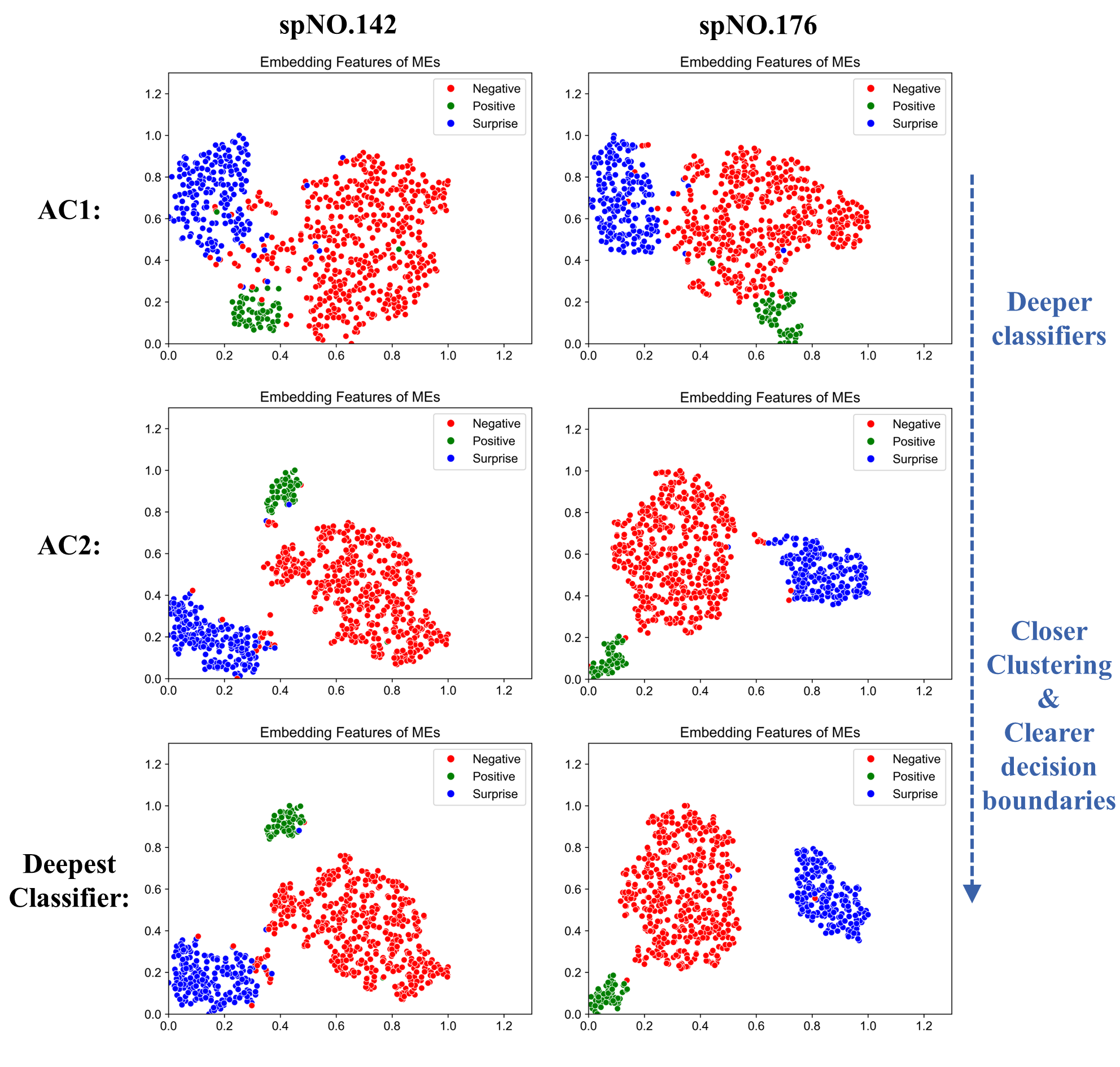
Figure 11: The t-SNE results of ME features generated by AC1, AC2, and the deepest classifier. The first and second columns are derived from subjects spNO.142 and spNO.176 in the CAS(ME)³ dataset, respectively.

for UAR compared to inputting 10 optical flow maps. The main reason is that the onset frame and offset frame represent the start and end of ME, while the apex frame represents the peak intensity of the expression. The optical flow maps between the three key-frames effectively reflect the motion information. After interpolation using TIM, the motion amplitude between adjacent frames is smaller, resulting in less distinct optical flow features and worse results.

4.5.5 More Analysis on the Performance of Different Classifiers

To verify that deeper classifiers in SKD extract more discriminative features, we compare the performance of each classifier on multiple datasets. As shown in Table 7, the deepest classifier 3/3 achieves the highest UF1 and UAR scores on different datasets. The deeper classifier 2/3 performs better than the shallow classifier 1/3, since the features extracted from the deeper

Table 7: Experimental results of different classifiers on multiple datasets.

Dataset	# Classes	Classifier 1/3		Classifier 2/3		Classifier 3/3
		UF1 (%)	UAR (%)	UF1 (%)	UAR (%)	UF1 (%)	UAR (%)
CASME II	5	75.00	74.61	87.80	87.98	90.34	89.47
	3	84.62	83.69	96.98	96.20	99.13	98.67
SAMM	3	68.66	68.24	86.13	84.34	94.29	92.65
MMEW	6	56.21	54.56	72.64	69.81	77.11	74.77
	4	71.43	71.96	88.47	88.33	90.41	90.44
CAS(ME)3	3	68.97	66.35	83.19	80.99	86.48	83.44
	4	52.39	51.68	73.27	70.14	76.40	72.57
	7	39.09	38.86	54.42	52.48	59.95	57.31

section are more discriminative. Although classifier 2/3 does not perform as well as the deepest classifier 3/3, its performance can also outperform other MER methods on different datasets, indicating the effectiveness of our SKD-TSTSAN. To visualize the discriminative features extracted by different classifiers, t-SNE is utilized to visualize the embedding ME features of subjects spNO.142 and spNO.176 in the CAS(ME)³ dataset, as shown in Fig. 11. It is obvious that the deeper classifiers have more concentrated clustering of the same category and clearer decision boundaries between different categories, indicating that more discriminative features are extracted.

5 Conclusion

In this paper, we propose a three-stream temporal-shift attention network based on self-knowledge distillation (SKD-TSTSAN) for ME recognition. First, we employ learning-based motion magnification modules to enhance muscle motion to make the ME features more discriminative. To suppress redundant information in the local-spatial stream and focus on important facial regions, we introduce a channel attention mechanism using the ECA modules. In addition, TSMs are incorporated into the dynamic-temporal stream for temporal modeling through information exchange in the temporal dimension. Furthermore, we introduce SKD into ME recognition by adding auxiliary classifiers into the network, taking the deepest part of the network as the teacher model for the shallower part and further improving the performance. Finally, extensive experiments on the CASME II, SAMM, MMEW, and CAS(ME)³ datasets show that our SKD-TSTSAN outperforms other cutting-edge MER methods.

In this paper, we classify MEs into a set of emotion categories using the onset frames, apex frames, and offset frames labeled in the dataset. However, to achieve an end-to-end ME analysis system, we still need to design an ME spotting method to identify key-frames. Therefore, in future work, we will explore ME spotting methods in long videos. Additionally, many current research efforts treat the ME spotting and recognition tasks separately [11]. However, these two tasks are strongly related and both require extracting subtle facial muscle motion features. Therefore, we will attempt to integrate ME spotting with our designed ME recognition network to implement ME analysis in a unified network.

References

- [1] Y. Li, J. Wei, Y. Liu, J. Kauttonen, G. Zhao, Deep learning for micro-expression recognition: A survey, IEEE Transactions on Affective Computing 13 (4) (2022) 2028–2046.
- [2] D. Matsumoto, H. S. Hwang, Evidence for training the ability to read microexpressions of emotion, Motivation and emotion 35 (2011) 181–191.
- [3] P. Ekman, Lie catching and microexpressions, The philosophy of deception 1 (2) (2009) 5.
- [4] S. Polikovsky, Y. Kameda, Y. Ohta, Facial micro-expressions recognition using high speed camera and 3d-gradient descriptor (2009).
- [5] T. Pfister, X. Li, G. Zhao, M. Pietikäinen, Recognising spontaneous facial micro-expressions, in: 2011 international conference on computer vision, IEEE, 2011, pp. 1449–1456.
- [6] Y.-J. Liu, J.-K. Zhang, W.-J. Yan, S.-J. Wang, G. Zhao, X. Fu, A main directional mean optical flow feature for spontaneous micro-expression recognition, IEEE Transactions on Affective Computing 7 (4) (2015) 299–310.
- [7] W.-J. Yan, X. Li, S.-J. Wang, G. Zhao, Y.-J. Liu, Y.-H. Chen, X. Fu, Casme ii: An improved spontaneous micro-expression database and the baseline evaluation, PloS one 9 (1) (2014) e86041.
- [8] A. K. Davison, C. Lansley, N. Costen, K. Tan, M. H. Yap, Samm: A spontaneous micro-facial movement dataset, IEEE transactions on affective computing 9 (1) (2016) 116–129.
- [9] X. Ben, Y. Ren, J. Zhang, S.-J. Wang, K. Kpalma, W. Meng, Y.-J. Liu, Video-based facial micro-expression analysis: A survey of datasets, features and algorithms, IEEE transactions on pattern analysis and machine intelligence 44 (9) (2021) 5826–5846.
- [10] J. Li, Z. Dong, S. Lu, S.-J. Wang, W.-J. Yan, Y. Ma, Y. Liu, C. Huang, X. Fu, Cas (me) 3: A third generation facial spontaneous micro-expression database with depth information and high ecological validity, IEEE Transactions on Pattern Analysis and Machine Intelligence 45 (3) (2022) 2782–2800.
- [11] B. Song, K. Li, Y. Zong, J. Zhu, W. Zheng, J. Shi, L. Zhao, Recognizing spontaneous micro-expression using a three-stream convolutional neural network, Ieee Access 7 (2019) 184537–184551.
- [12] B. Xia, S. Wang, Micro-expression recognition enhanced by macro-expression from spatial-temporal domain., in: IJCAI, 2021, pp. 1186–1193.
- [13] T.-H. Oh, R. Jaroensri, C. Kim, M. Elgharib, F. Durand, W. T. Freeman, W. Matusik, Learning-based video motion magnification, in: Proceedings of the European Conference on Computer Vision (ECCV), 2018, pp. 633–648.
- [14] Q. Wang, B. Wu, P. Zhu, P. Li, W. Zuo, Q. Hu, Eca-net: Efficient channel attention for deep convolutional neural networks, in: Proceedings of the IEEE/CVF conference on computer vision and pattern recognition, 2020, pp. 11534–11542.
- [15] J. Lin, C. Gan, S. Han, Tsm: Temporal shift module for efficient video understanding, in: Proceedings of the IEEE/CVF international conference on computer vision, 2019, pp. 7083–7093.
- [16] P. Lucey, J. F. Cohn, T. Kanade, J. Saragih, Z. Ambadar, I. Matthews, The extended cohn-kanade dataset (ck+): A complete dataset for action unit and emotion-specified expression, in: 2010 ieee computer society conference on computer vision and pattern recognition-workshops, IEEE, 2010, pp. 94–101.
- [17] L. Zhang, J. Song, A. Gao, J. Chen, C. Bao, K. Ma, Be your own teacher: Improve the performance of convolutional neural networks via self distillation, in: Proceedings of the IEEE/CVF international conference on computer vision, 2019, pp. 3713–3722.
- [18] R. Chaudhry, A. Ravichandran, G. Hager, R. Vidal, Histograms of oriented optical flow and binet-cauchy kernels on nonlinear dynamical systems for the recognition of human actions, in: 2009 IEEE conference on computer vision and pattern recognition, IEEE, 2009, pp. 1932–1939.
- [19] S. Zhang, B. Feng, Z. Chen, X. Huang, Micro-expression recognition by aggregating local spatio-temporal patterns, in: MultiMedia Modeling: 23rd International Conference, MMM 2017, Reykjavik, Iceland, January 4-6, 2017, Proceedings, Part I 23, Springer, 2017, pp. 638–648.
- [20] S.-J. Wang, W.-J. Yan, X. Li, G. Zhao, C.-G. Zhou, X. Fu, M. Yang, J. Tao, Micro-expression recognition using color spaces, IEEE Transactions on Image Processing 24 (12) (2015) 6034–6047.
- [21] F. Xu, J. Zhang, J. Z. Wang, Microexpression identification and categorization using a facial dynamics map, IEEE Transactions on Affective Computing 8 (2) (2017) 254–267.
- [22] Y. Wang, J. See, R. C.-W. Phan, Y.-H. Oh, Lbp with six intersection points: Reducing redundant information in lbp-top for micro-expression recognition, in: Computer Vision–ACCV 2014: 12th Asian Conference on Computer Vision, Singapore, Singapore, November 1-5, 2014, Revised Selected Papers, Part I 12, Springer, 2015, pp. 525–537.
- [23] Z. Wang, K. Zhang, W. Luo, R. Sankaranarayana, Htnet for micro-expression recognition, arXiv preprint arXiv:2307.14637 (2023).
- [24] L. Lei, J. Li, T. Chen, S. Li, A novel graph-tcn with a graph structured representation for micro-expression recognition, in: Proceedings of the 28th ACM International Conference on Multimedia, 2020, pp. 2237–2245.
- [25] J. Zhang, B. Yan, X. Du, Q. Guo, R. Hao, J. Liu, L. Liu, G. Ni, X. Weng, Y. Liu, Motion magnification multi-feature relation network for facial microexpression recognition, Complex & Intelligent Systems 8 (4) (2022) 3363–3376.
- [26] M. Wei, W. Zheng, Y. Zong, X. Jiang, C. Lu, J. Liu, A novel micro-expression recognition approach using attention-based magnification-adaptive networks, in: ICASSP 2022-2022 IEEE International Conference on Acoustics, Speech and Signal Processing (ICASSP), IEEE, 2022, pp. 2420–2424.
- [27] S.-J. Wang, B.-J. Li, Y.-J. Liu, W.-J. Yan, X. Ou, X. Huang, F. Xu, X. Fu, Micro-expression recognition with small sample size by transferring long-term convolutional neural network, Neurocomputing 312 (2018) 251–262.
- [28] J. Li, Y. Wang, J. See, W. Liu, Micro-expression recognition based on 3d flow convolutional neural network, Pattern Analysis and Applications 22 (2019) 1331–1339.
- [29] H.-X. Xie, L. Lo, H.-H. Shuai, W.-H. Cheng, Au-assisted graph attention convolutional network for micro-expression recognition, in: Proceedings of the 28th ACM International Conference on Multimedia, 2020, pp. 2871–2880.
- [30] C. Wu, F. Guo, Tsnn: Three-stream combining 2d and 3d convolutional neural network for micro-expression recognition, IEEJ Transactions on Electrical and Electronic Engineering 16 (1) (2021) 98–107.
- [31] H.-Q. Khor, J. See, R. C. W. Phan, W. Lin, Enriched long-term recurrent convolutional network for facial micro-expression recognition, in: 2018 13th IEEE international conference on automatic face & gesture recognition (FG 2018), IEEE, 2018, pp. 667–674.
- [32] F. A. Gers, J. Schmidhuber, F. Cummins, Learning to forget: Continual prediction with lstm, Neural computation 12 (10) (2000) 2451–2471.
- [33] G. Hinton, O. Vinyals, J. Dean, Distilling the knowledge in a neural network, arXiv preprint arXiv:1503.02531 (2015).
- [34] B. Sun, S. Cao, D. Li, J. He, L. Yu, Dynamic micro-expression recognition using knowledge distillation, IEEE Transactions on Affective Computing 13 (2) (2020) 1037–1043.
- [35] J. Hu, L. Shen, G. Sun, Squeeze-and-excitation networks, in: Proceedings of the IEEE conference on computer vision and pattern recognition, 2018, pp. 7132–7141.
- [36] T.-Y. Lin, P. Goyal, R. Girshick, K. He, P. Dollár, Focal loss for dense object detection, in: Proceedings of the IEEE international conference on computer vision, 2017, pp. 2980–2988.
- [37] J. Deng, J. Guo, Y. Zhou, J. Yu, I. Kotsia, S. Zafeiriou, Retinaface: Single-stage dense face localisation in the wild, arXiv preprint arXiv:1905.00641 (2019).
- [38] C. Zach, T. Pock, H. Bischof, A duality based approach for realtime tv-l 1 optical flow, in: Pattern Recognition: 29th DAGM Symposium, Heidelberg, Germany, September 12-14, 2007. Proceedings 29, Springer, 2007, pp. 214–223.
- [39] A. J. R. Kumar, B. Bhanu, Micro-expression classification based on landmark relations with graph attention convolutional network, in: Proceedings of the IEEE/CVF conference on computer vision and pattern recognition, 2021, pp. 1511–1520.
- [40] J. Liu, W. Zheng, Y. Zong, Sma-stn: Segmented movement-attending spatiotemporal network formicro-expression recognition, arXiv preprint arXiv:2010.09342 (2020).
- [41] X.-B. Nguyen, C. N. Duong, X. Li, S. Gauch, H.-S. Seo, K. Luu, Micron-bert: Bert-based facial micro-expression recognition, in: Proceedings of the IEEE/CVF Conference on Computer Vision and Pattern Recognition, 2023, pp. 1482–1492.
- [42] S.-T. Liong, Y. S. Gan, J. See, H.-Q. Khor, Y.-C. Huang, Shallow triple stream three-dimensional cnn (ststnet) for micro-expression recognition, in: 2019 14th IEEE international conference on automatic face & gesture recognition (FG 2019), IEEE, 2019, pp. 1–5.
- [43] Y. S. Gan, S.-T. Liong, W.-C. Yau, Y.-C. Huang, L.-K. Tan, Off-apexnet on micro-expression recognition system, Signal Processing: Image Communication 74 (2019) 129–139.
- [44] Y. Liu, H. Du, L. Zheng, T. Gedeon, A neural micro-expression recognizer, in: 2019 14th IEEE international conference on automatic face & gesture recognition (FG 2019), IEEE, 2019, pp. 1–4.
- [45] L. Zhou, Q. Mao, X. Huang, F. Zhang, Z. Zhang, Feature refinement: An expression-specific feature learning and fusion method for micro-expression recognition, Pattern Recognition 122 (2022) 108275.
- [46] N. Van Quang, J. Chun, T. Tokuyama, Capsulenet for micro-expression recognition, in: 2019 14th IEEE International Conference on Automatic Face & Gesture Recognition (FG 2019), IEEE, 2019, pp. 1–7.
- [47] H. Li, M. Sui, Z. Zhu, F. Zhao, Mmnet: Muscle motion-guided network for micro-expression recognition, arXiv preprint arXiv:2201.05297 (2022).
- [48] Z. Xia, W. Peng, H.-Q. Khor, X. Feng, G. Zhao, Revealing the invisible with model and data shrinking for composite-database micro-expression recognition, IEEE Transactions on Image Processing 29 (2020) 8590–8605.
- [49] G.-B. Liong, S.-T. Liong, C. S. Chan, J. See, Sfamnet: A scene flow attention-based micro-expression network, Neurocomputing 566 (2024) 126998.
- [50] R. R. Selvaraju, M. Cogswell, A. Das, R. Vedantam, D. Parikh, D. Batra, Grad-cam: Visual explanations from deep networks via gradient-based localization, in: Proceedings of the IEEE international conference on computer vision, 2017, pp. 618–626.