Playing with Fire? A Mean Field Game Analysis of Fire Sales and Systemic Risk under Regulatory Capital Constraints

Abstract.

We study the impact of regulatory capital constraints on fire sales and financial stability in a large banking system using a mean field game model. In our model banks adjust their holdings of a risky asset via trading strategies with finite trading rate in order to maximize expected profits. Moreover, a bank is liquidated if it violates a stylized regulatory capital constraint. We assume that the drift of the asset value is affected by the average change in the position of the banks in the system. This creates strategic interaction between the trading behavior of banks and thus leads to a game. The equilibria of this game are characterized by a system of coupled PDEs. We solve this system explicitly for a test case without regulatory constraints and numerically for the regulated case. We find that capital constraints can lead to a systemic crisis where a substantial proportion of the banking system defaults simultaneously. Moreover, we discuss proposals from the literature on macroprudential regulation. In particular, we show that in our setup a systemic crisis does not arise if the banking system is sufficiently well capitalized or if improved mechanisms for the resolution of banks violating the risk capital constraints are in place.

Keywords: Mean field game , Systemic risk, Price-mediated contagion, Risk capital constraints, McKean-Vlasov equation

1. Introduction

Contagious interactions between financial institutions play an important role in the amplification of economic shocks during a financial crisis. A prime example is the global financial crisis of 2007-2009, where comparatively small losses on the market for US subprime mortgages were magnified by the financial system and caused a major recession whose repercussions were felt throughout the globe. This has led to a large literature on financial contagion and systemic risk. Most of this work focuses on direct contagion generated by contractual links between financial institutions such as interbank lending or OTC derivatives. Examples of this line of research include Eisenberg and Noe [14], Elsinger et al. [15], Rogers and Veraart [25], Glasserman and Young [18] or Frey and Hledik [17]. Indirect or price-mediated contagion on the other hand is caused by price effects due to forced de-leveraging, where a distressed financial institution is rapidly selling some of its risky assets in order to stay solvent or to comply with regulatory constraints in so-called fire sales. These fire sales tend to exhaust demand for risky assets, which pushes asset prices downward and possibly leads to losses of other financial institutions as well. The relevance of price-mediated contagion is stressed in many reports and policy papers on the great financial crisis, see Hanson et al. [21] or the introduction of Braouezec and Wagalath [5]. In particular, in [4] the Basel committee acknowledges that

at the height of the crisis financial markets forced the banking sector to reduce its leverage in a manner that amplified downward pressures on asset prices. This de-leveraging process exacerbated the feedback loop between losses, falling bank capital and shrinking credit availability.

According to the literature on macroprudential regulation such as Hanson et al. [21], regulatory capital constraints may be an important contributor to price-mediated contagion: under the Basel capital adequacy framework the risk capital of a bank (its equity and certain forms of long-term debt) must exceed a multiple of its risk weighted assets (a measure of the overall size of the risky assets of a bank scaled by their relative riskiness). If a bank incurs substantial losses, its risk capital might be reduced tho the extent that it no longer complies with the Basel rules. Since in such a situation it is usually too costly to issue new equity, the bank is forced to engage in fire sales in order to avoid regulatory penalties or liquidation. In a recession scenario where many banks experience losses simultaneously, these fire sales might destabilize the banking system via price mediated contagion.

Despite the relevance of the topic there are only few mathematical models that analyze the implications of regulatory capital constraints for systemic risk, see the literature review below. In this paper we analyze price-mediated contagion in the context of a mean field game model for a large banking system. In our setup a bank invests into a non-tradable asset, for instance retail loans, into a tradable but illiquid risky asset, for instance tradable credit positions and in cash, with the objective of maximizing the expected value of its equity at some horizon date $T$. The position in the tradable asset can be adjusted only gradually, so that we confine banks to trading strategies that are absolutely continuous with a finite trading rate. Moreover, banks incur transaction costs which depend on the size of the trading rate, making a very rapid adjustment of their position prohibitively costly. We assume that the drift of the tradable assets depends on the change in the average asset holdings of the banks in the system. In particular prices are pushed downward if the banking sector reduces its overall position in the tradable assets, so that there is price-mediated contagion. The optimal trading rate of a bank obviously depends on the drift of the risky asset and hence on the trading strategies of the other banks, so that there is interaction between their trading strategies. In mathematical terms we are dealing with a so-called mean-field game of controls (MFGC), where agents interact via the distribution of their states and via the distribution of the controls (in our case their trading strategies). We introduce a stylized risk capital constraint and impose the condition that the equity value of a bank needs to exceed a multiple of its asset holdings at all times. Upon violation of this condition a bank is liquidated by regulators and its assets are sold on the market.

In the case without capital constraints the mathematical structure of our model is similar to the MFGC used by Cardaliaguet and LeHalle [6] to study strategic interaction in optimal portfolio execution. In particular, the PDE system for the game (the dynamic programming equation for the control problem of individual banks and the forward equation for the distribution of bank characteristics) can be reduced to a system of ODEs that has an explicit solution. In the case with capital constraints, on the other hand, the PDE system for the mean field game becomes a boundary value problem for which there is no explicit solution. Hence we have to resort to numerical methods. The numerical analysis of the PDE system corresponding to a MFG is challenging since one deals simultaneously with a forward and a backward equation and hence with a fixed point problem. For our MFGC model we use Picard iterations combined with a special discretization scheme that uses some ideas from Achdou and Laurière [2].

Using this scheme we study numerically the impact of capital constraints case on the stability of the banking system. We find that banks liquidate their position faster than in the unregulated case, in particular when they are close to the liquidation boundary, and that they hold on average a lower amount of the risky asset, so that the risk bearing capacity of the banking system is reduced by the capital constraints. For certain parameter values we observe a liquidation cascade where many banks are violating the risk capital constraints more or less simultaneously and where the ensuing fire sales have a substantial impact on the drift of the risky assets. These findings lends formal support to the conjecture from the regulatory literature that risk capital constraints may cause price-mediated contagion. With this in mind we test several macroprudential risk management policies (regulatory measures trying to mitigate the external effects of rapid deleveraging by multiple financial institutions) from the regulatory literature, see Hanson et al. [21]). In particular, we find that in our setup the adverse effects of capital constraints disappear if the banking system is sufficiently well capitalized. Moreover, we show that financial stability is enhanced if banks violating the capital constraints are resolved in a way that mitigates price-mediated contagion, for instance by parking their assets in a special purpose vehicle that is unwound only gradually over time.

The remainder of the paper is organized as follows. In Section 2 we introduce our setup and the optimization problem of an individual bank. The case without capital constraints, where the MFGC has an explicit solution, is studied in Section 3. In Section 4 we discuss the PDE system for the MFGC model with capital constraints. Numerical experiments studying the implications of capital constraints for financial stability are discussed in Section 5.

Literature review.

We begin with the literature that studies the implications of regulatory capital constraints in formal economic models. Braouezec and Wagalath [5] consider a one period model with finitely many banks that hold positions in the same risky asset. They assume that the value of this asset is hit by an exogenous shock at time $t=1$ and that every bank sells the minimal amount of assets necessary to comply with the Basel rules. The market for the asset is not perfectly liquid. Hence the fire sales of one bank create an externality for the other banks in the system and the liquidation problem becomes a game. Braouezec and Wagalath [5] prove that this game has at least one equilibrium. Moreover, they run simulation experiments with input data calibrated to the American banking system, which show that in their model price mediated contagion significantly amplifies the impact of the initial shock. Feinstein [16] extends this analysis to a setting in continuous time with deterministic asset prices. We stress that in these models banks react in a quite mechanical way to the risk capital constraints. In our model on the other hand, risk capital constraints and the ensuing price-mediated contagion are factored into the dynamic investment strategies of the banks and influence their behavior prior to reaching the liquidation boundary. For further work on fire sales and price-mediated contagion we refer to Cont and Wagalath [10] or Cont and Schaanning [11] and the references therein.

Next we discuss mean field game models for systemic risk. A simple model is proposed in Carmona et al. [9]. More relevant for our work are the papers by Nadtochiy and Shkolnikov [24], Hambly et al. [20], [19] or Cuchiero et al. [12]. These papers extend the neuron-firing model of Delarue et al. [13] to systemic risk. More precisely, they study the mean field limit of banking systems where every bank suffers a loss if one bank in the system crosses an exogeneous default barrier. Fundamental contributions on mean field games include Lasry and Lions [22, 23] and Carmona and Delarue [8]. Lasry and Lions [22, 23] focus on the PDE approach (as we do in the present paper) whereas Carmona and Delarue [8] discuss the probabilistic approach based on forward backward SDEs. A good general introduction to the topic is given in Cardaliaguet and Porretta [7].

2. The Model

2.1. The Banking System

Fix some horizon date $T$. We consider a large banking system with a continuum $I$ of stylized banks. Each bank $i\in I$ holds some non-tradable asset with value $A^{i}$, for instance retail loans. Moreover, it invests into a risky asset $S^{i}$, for instance tradable credit positions, and in cash. We assume that the market for the asset $S^{i}$ is not perfectly liquid so that a bank can adjust its position only gradually over time. In mathematical terms it is restricted to trading strategies with finite trading rate $\boldsymbol{\nu}^{i}=(\nu_{t}^{i})_{0\leq t\leq T}$. Moreover, there are transaction costs that are proportional to $(\nu_{t}^{i})^{2}$; in this way we penalize a very rapid change of positions. We denote by $Q^{i}=(Q_{t}^{i})_{0\leq t\leq T}$ the amount of the tradable risky assets held by bank $i$ (also referred to as inventory level) and by $C^{i}=(C_{t}^{i})_{0\leq t\leq T}$ its cash position. We allow for $C_{t}^{i}<0$ (this corresponds to the case where the bank is a net borrower) and we work for simplicity with an interest rate $r=0$.

For a given trading strategy $\boldsymbol{\nu}$, the the dynamics of $(A^{i},Q^{i},S^{i})$ are

(2.1) $$\mathrm{d}A_{t}^{i} =\sigma_{A}\mathrm{d}W_{t}^{A,i}$$

(2.2) $$\mathrm{d}Q_{t}^{i} =\nu_{t}^{i}\mathrm{d}t+{\sigma_{Q}\mathrm{d}{W}_{t}^{Q,i}}$$

(2.3) $$\mathrm{d}S_{t}^{i} =(\mu_{\text{ex}}+\alpha\overline{\mu}_{t})\mathrm{d}t+\sigma_{S}\mathrm{d}W_{t}^{i}$$

for parameters $\alpha,\sigma_{A},\sigma_{S},\sigma_{Q}\geq 0$ and a three-dimensional standard Brownian motion $\mathbf{W}^{i}=(W^{Q,i},W^{A,i},W^{S,i})$. The transaction cost incurred by bank $i$ is given by $\kappa(\nu_{t}^{i})^{2}$ for some $\kappa>0$. We assume that the trading strategies used by bank $i$ will be adapted to the filtration generated by the Brownian motion $\mathbf{W}^{i}$ and sufficiently integrable, that is $\int_{0}^{T}\left(\nu_{s}^{i}\right)^{2}\mathrm{d}s<\infty$. Moreover, the Brownian motions are independent across banks. The cash account is used to finance the trading activities of the bank and it collects proceeds from asset sales; its dynamics are thus given by

$$\mathrm{d}C_{t}^{i}=-S_{t}^{i}\mathrm{d}Q_{t}^{i}-\kappa\left(\nu_{t}^{i}\right)^{2}\mathrm{d}t.$$

Denote by

(2.4) $$X_{t}^{i,\boldsymbol{\nu}}=A_{t}^{i}+S_{t}^{i}Q_{t}^{i,\boldsymbol{\nu}}+C_{t}^{i,\boldsymbol{\nu}}$$

the value of the equity of bank $i$ given that it uses the trading strategy $\boldsymbol{\nu}$. Banks choose their trading rate $\boldsymbol{\nu}$ in order to maximize their expected equity value at the horizon date $T$, $\mathbb{E}\big{(}X_{T}^{i,\boldsymbol{\nu}}\big{)}$, over all strategies $\boldsymbol{\nu}$. For comparison purposes, in the case without capital constraints we also consider the more general problem of maximizing $\mathbb{E}\left(X_{T}^{i,\boldsymbol{\nu}}-\gamma\big{(}Q_{T}^{i,\boldsymbol{\nu}}\big{)}^{2}\right)$ for some $\gamma>0$, where the penalty $\gamma(Q_{T}^{i,\boldsymbol{\nu}})^{2}$ can be interpreted as a terminal liquidation cost.

Comments.

(i) The drift of $S^{i}$ depends on two components: $\mu_{\text{ex}}$ represents some exogenous trend and the interaction or contagion term $\overline{\mu}_{t}$ is the rate of change in the average number of risky assets held by the banking sector (a precise definition is given in (3.4) and (4.3) below). In particular the drift of $S^{i}$ decreases if the banking sector reduces its overall position in the tradable assets. Note that the optimal trading rate of bank $i$ depends on the drift of $S^{i}$ and hence on the contagion term $\overline{\mu}_{t}$, which in turn depends on the trading strategies of the other banks in the system. Hence there is strategic interaction between the trading of the banks and are dealing with a game.

(ii) The diffusion term in the dynamics of $Q^{i}$ reflects the fact that large banks are usually not able to perfectly control the exact amount of risky assets they hold, for instance due to execution delays. From a mathematical perspective, the diffusion term in the dynamics of $A^{i}$ and $Q^{i}$ ensures that the PDE system characterizing the mean-field game is uniformly parabolic.

(ii) In our model the Brownian motions $\mathbf{W}^{i}$, $i\in I$, are independent, so that banks interact only via the impact of their trading on the drift $\overline{\mu}$. It might make sense to consider a common noise component in the asset price, but this more involved case is left for future research.

2.2. The HJB equation

Next we derive the HJB equation for the optimization problem of a generic bank. From now on we omit the superscript $i$ since the banks in our system are all identical. Using Itô’s product formula and the assumption that Brownian motions are independent we get the following dynamics for the process $\mathbf{X}=(Q,X)$,

$$\mathrm{d}Q_{t} =\nu_{t}\mathrm{d}t+\sigma_{Q}\mathrm{d}W_{t}^{Q},$$

$$\mathrm{d}X_{t} =\mathrm{d}A_{t}+\mathrm{d}(S_{t}Q_{t})+\mathrm{d}C_{t}=\mathrm{d}A_{t}+Q_{t}\mathrm{d}S_{t}+S_{t}\mathrm{d}Q_{t}-S_{t}\mathrm{d}Q_{t}-\kappa\nu_{t}^{2}\mathrm{d}t$$

$$=\left(Q_{t}(\mu_{\text{ex}}+\alpha\overline{\mu}_{t})-\kappa\nu_{t}^{2}\right)\mathrm{d}t+\sigma_{A}\mathrm{d}W_{t}^{A}+Q_{t}\sigma_{S}\mathrm{d}W_{t}^{S}.$$

Assume furthermore that $\overline{\mu}_{t}$ is given by a known function $\mu(t)$ ($\mu(t)$ can be interpreted as a bank’s expectation of the contagion term.) It follows that for a constant strategy $\nu_{t}\equiv\nu$ the process $\mathbf{X}$ is Markov with generator

$$\mathcal{L}^{\mathbf{X},\nu}f=\nu\partial_{q}f+\left(q(\mu_{\text{ex}}+\alpha\mu(t))-\kappa\nu^{2}\right)\partial_{x}f+\frac{1}{2}\sigma_{Q}^{2}\partial_{q}^{2}f+\frac{1}{2}\left(\sigma_{A}^{2}+\sigma_{S}^{2}q^{2}\right)\partial_{x}^{2}f.$$

Standard arguments of stochastic control theory give the following HJB equation for the value function $u$ of the bank’s optimization problem

$$0=\partial_{t}u+\sup_{\nu\in\mathbb{R}}\left\{\nu\partial_{q}u+\left(q(\mu_{\text{ex}}+\alpha\mu)-\kappa\nu^{2}\right)\partial_{x}u+\frac{1}{2}\sigma_{Q}^{2}\partial_{q}^{2}u+\frac{1}{2}\left(\sigma_{A}^{2}+\sigma_{S}^{2}q^{2}\right)\partial_{x}^{2}u\right\},$$

or, equivalently,

(2.5) $$0 =\partial_{t}u+q(\mu_{\text{ex}}+\alpha\mu(t))\partial_{x}u+\frac{1}{2}\sigma_{Q}^{2}\partial_{q}^{2}u+\frac{1}{2}\left(\sigma_{A}^{2}+\sigma_{S}^{2}q^{2}\right)\partial_{x}^{2}u+\sup_{\nu\in\mathbb{R}}\left\{\nu\partial_{q}u-\kappa\nu^{2}\partial_{x}u\right\}\,;$$

the terminal condition is $u(T,q,x)=x-\gamma q^{2}.$ Note that in an equilibrium of the game the predicted drift $\mu(t)$ and the realized drift $\overline{\mu}_{t}$ should coincide so that we get the additional consistency or equilibrium condition $\mu(t)=\overline{\mu}_{t}$.

2.3. Risk capital constraints

Under the Basel capital adequacy rules the risk capital of a bank must exceed a multiple of its so-called risk weighted assets (RWA). Loosely speaking, this quantity is a weighted average of the size of the position in different asset classes, where the weights reflect differences in riskiness. In this paper we introduce a stylized version of this constraint. We model the risk capital of a bank at time $t$ by the book value of its equity $X_{t}$ and the risk weighted assets by the term $\tilde{\beta}|Q_{t}|+\tilde{c}$ where $\tilde{\beta}|Q_{t}|$ represents the risk of the position in the tradable asset $S$ and the constant $\tilde{c}$ the risk of the position in the non-traded asset. This leads to a condition of the form $X_{t}>\beta|Q_{t}|+c$ for constants $c,\beta>0$. We denote by the open set $\mathcal{A}$ the set of acceptable positions, that is

(2.6) $$\mathcal{A}=\{\mathbf{x}=(q,x)\in\mathbb{R}\times\mathbb{R}^{+}\colon x>\beta|q|+c\}$$

and we we denote its boundary by $\partial\mathcal{A}$. In the case with capital constraints we assume that a bank is liquidated by the regulator at the stopping time $\tau=\inf\{t\geq 0\colon\mathbf{X}_{t}\notin\mathcal{A}\}$, that is as soon as its position reaches $\partial\mathcal{A}$. We assume that the equity holders lose their claim to the bank’s equity in that case. This leads to the boundary condition $u\equiv 0$ on $\partial\mathcal{A}$. (For mathematical reasons, in Section 4 we will consider a slightly relaxed version of this condition.) In the sequel we refer to a bank with $\tau>t$ as an active bank at $t$.

3. The Case without Capital Constraints

In the case without capital constraints (the so-called unregulated case) we denote the value function by $u^{\text{unreg}}$. Choosing a similar approach as Cardaliaguet and LeHalle [6], we obtain an explicit solution for $u^{\text{unreg}}$ and for the optimal strategy. We make the Ansatz $u^{\text{unreg}}(t,q,x)=x+v(t,q)$. This implies that $\partial_{x}u^{\text{unreg}}=1$ and we get the following HJB equation for $v$ (for a given interaction term $\mu(t)$)

(3.1) $$0=\partial_{t}v+q(\alpha\mu(t)+\mu_{\text{ex}})+\sup_{\nu\in\mathbb{R}}\left\{\nu\partial_{q}v-\kappa\nu^{2}\right\},$$

with terminal condition $v(T,q)=-\gamma q^{2}$. It follows that the optimal strategy is given by

(3.2) $$\nu^{*}(t,q)=\frac{\partial_{q}v(t,q)}{2\kappa},$$

in particular, $\nu^{*}$ is independent of $x$. To find an explicit solution for $v$ we make the Ansatz

$$v(t,q)=h_{0}(t)+h_{1}(t)q-\frac{1}{2}h_{2}(t)q^{2}.$$

Note that $\sup_{\nu\in\mathbb{R}}\left\{\nu\partial_{q}v-\kappa\nu^{2}\right\}=\frac{(\partial_{q}v)^{2}}{4\kappa}$. Substituting the Ansatz for $v$ into the HJB (3.1) gives

$$0=h_{0}^{\prime}+h_{1}^{\prime}q-\frac{1}{2}h_{2}^{\prime}q^{2}+q(\alpha\mu(t)+\mu_{\text{ex}})+\frac{h_{1}^{2}-2h_{1}h_{2}q+h_{2}^{2}q^{2}}{4\kappa},$$

which yields the following ODE system for $h_{0},h_{1},h_{2}$

$$h_{2}^{\prime} =\frac{h_{2}^{2}}{2\kappa},\quad h_{1}^{\prime}=-\alpha\mu(t)-\mu_{\text{ex}}+\frac{h_{1}h_{2}}{2\kappa},\quad h_{0}^{\prime}=-\frac{h_{1}^{2}}{4\kappa}$$

with terminal conditions $h_{0}(T)=h_{1}(T)=0$ and $h_{2}(T)=2\gamma$. There is an explicit solution of the ODE for $h_{2}$,

(3.3) $$\begin{cases}h_{2}(t)=\frac{2\kappa}{T-t+\frac{\kappa}{\gamma}}&\gamma>0,\\ h_{2}(t)\equiv 0&\gamma=0.\end{cases}$$

Moreover, the optimal strategy is given by $\nu^{*}(t,q)=\frac{1}{2\kappa}(h_{1}(t)-h_{2}(t)q)$. Note that this strategy is linear in $q$ (and in fact even constant if $\gamma=0$).

Since $\nu^{*}$ depends only on $q$ (and not on the equity value $x$), each agent is fully characterized by his current inventory, so that we may describe the distribution of agents in terms of the distribution of inventory levels. We denote the distribution of $Q_{t}$ $m_{t}(\mathrm{d}q)$ and we use for $f:\mathbb{R}\to\mathbb{R}$ the notation $\langle m_{t},f\rangle:=\int_{\mathbb{R}}f(q)m(t,\mathrm{d}q)$. Recall that the interaction term in the drift is of the assets is the change in the average inventory level. Using the above notation we get the following formal definition of $\overline{\mu}_{t}$

(3.4) $$\overline{\mu}_{t}=\int_{\mathbb{R}}q\,m(t,\mathrm{d}q)=\langle m(t),q\rangle\,.$$

Denote by $\mathcal{L}^{Q}$ the generator of $Q$. For $f$ in the domain of $\mathcal{L}^{Q}$ the weak form of the forward equation for the evolution of $m_{t}(\mathrm{d}q)$ reads

$$\partial_{t}\langle m_{t},f\rangle=\langle m_{t},\mathcal{L}_{t}^{Q}f\rangle\,.$$

If $m_{t}(\mathrm{d}q)$ has a density, i.e. $m(t,\mathrm{d}q)=m(t,q)\mathrm{d}q$ for all $t$, partial integration gives the classical forward equation for $m(t,q)$ (but in the case without capital constraints we do not need this equation). Using the forward equation and the fact that $\mathcal{L}^{Q}q=\nu^{*}$ we get that

(3.5) $$\overline{\mu}_{t}=\partial_{t}\langle m_{t},q\rangle=\langle m(t),\mathcal{L}_{t}^{Q}q\rangle=\langle m_{t},\nu^{*}(t,\cdot)\rangle\,,$$

so that $\overline{\mu}$ can be interpreted as average trading rate of the banks.

Following [6], we introduce the average inventory level $E(t)=\langle m(t),q\rangle$. It follows from (3.4) that the contagion term $\overline{\mu}_{t}$ equals $E^{\prime}(t)$. Using (3.5) and the relation $\nu^{*}(t,q)=\frac{1}{2\kappa}(h_{1}(t)-h_{2}(t)q)$ we thus get the following ODE for the average inventory $E(t)$

$$E^{\prime}(t)=\langle m_{t},\nu^{*}(t,\cdot)\rangle=\frac{1}{2\kappa}\left(h_{1}(t)-h_{2}(t)E(t)\right)\,,$$

with initial condition $E_{0}=\langle m_{0},q\rangle$, where $m_{0}(\mathrm{d}q)$ is the given initial distribution of the inventory $Q$. Using finally the equilibrium condition $\mu(t)=\overline{\mu}_{t}$, we get the following ODE system for $h_{0},h_{1}$ and $E$ ($h_{2}$ is given in (3.3))

(3.6a) $$h_{1}^{\prime} =-\frac{\alpha}{2\kappa}\left(h_{1}-h_{2}E\right)-\mu_{\text{ex}}+\frac{h_{1}h_{2}}{2\kappa} h_{1}(T)=0\,,$$

(3.6b) $$h_{0}^{\prime} =-\frac{h_{1}^{2}}{4\kappa} h_{0}(T)=0\,,$$

(3.6c) $$E^{\prime} =\frac{1}{2\kappa}\left(h_{1}-h_{2}E\right) E(0)=E_{0}.$$

The ODE system (3.4) can be viewed as a reduced form of the PDE system that usually describes the equilibrium in a MFG. In fact, the backward equation (3.6a) derives from the HJB equation and it ensures that trading rate of a bank is optimal given the interaction term whereas (3.6c) comes from the forward equation for the distribution of the inventory.

Next we extend the arguments from [6] to obtain an explicit solution. We get from (3.6c) that $h_{1}=2\kappa E^{\prime}+h_{2}E,$ and hence $h_{1}^{\prime}=2\kappa E^{\prime\prime}+h_{2}^{\prime}E+h_{2}E^{\prime}.$ Plugging the second relation into (3.6a) yields

$$0 =-(2\kappa E^{\prime\prime}+h_{2}^{\prime}E+h_{2}E^{\prime})-\alpha E^{\prime}-\mu_{\text{ex}}+E^{\prime}h_{2}+\frac{h_{2}^{2}E}{2\kappa}$$

$$=-2\kappa E^{\prime\prime}-\alpha E^{\prime}+\frac{h_{2}^{2}-2\kappa h_{2}^{\prime}}{2\kappa}E-\mu_{\text{ex}}.$$

By (3.3), we get the following second order ODE for $E$

(3.7) $$E^{\prime\prime}+\frac{\alpha}{2\kappa}E^{\prime}=-\frac{\mu_{\text{ex}}}{2\kappa},$$

with initial condition $E(0)=E_{0}$ and with $E(T)$ solving $E^{\prime}(T)+\frac{\gamma}{\kappa}E(T)=0$ (this follows from (3.6c)). Solving this problem yields

$$E(t)=\frac{E_{0}\left(\alpha^{2}e^{-\frac{\alpha}{2\kappa}T}+2\gamma\alpha\left(e^{-\frac{\alpha}{2\kappa}t}-e^{-\frac{\alpha}{2\kappa}T}\right)\right)-\left(2\kappa\mu_{\text{ex}}+2\mu_{\text{ex}}\gamma T\right)\left(e^{-\frac{\alpha}{2\kappa}t}-1\right)}{\left(\alpha^{2}-2\gamma\alpha\right)e^{-\frac{\alpha}{2\kappa}T}+2\gamma\alpha}-\frac{\mu_{\text{ex}}}{\alpha}t.$$

Given $h_{2}$ and $E$, we can compute $h_{1}$, $h_{0}$ and therefore also $v$ and $\nu^{*}$ by integration. The corresponding formulas are given in Appendix B.

4. The case with capital constraints

4.1. The PDE system for the MFGC

In the case with capital constraints the Ansatz $u(t,q,x)=x+v(t,q)$ is inconsistent with the boundary condition for $u$ on $\partial\mathcal{A}$. Moreover, we expect that the optimal trading rate depends both on $x$ and $q$, since close to the boundary of $\mathcal{A}$ the bank will want to reduce its position in order to avoid liquidation. Hence we need to work with the two-dimensional state price process $\mathbf{X}=(X,Q)$ and with the full HJB equation (2.5).

To complete the description of the HJB equation in the case with capital constraints we next give a precise description of the terminal and boundary condition we impose on $u$. At $T$ we assume that $u(T,x,q)=x$. Consider next for fixed $\epsilon>0$ the function $k\colon[0,T]\to\mathbb{R}$ with

$$k(t)=\frac{1}{2\epsilon}\left(t-T+\epsilon+\sqrt{0.0004+(t-T+\epsilon)^{2}}\right),$$

and note that $k$ is a smooth function with the following properties: $k(T)\approx 1$; $k(t)$ is non-decreasing for all $t\leq T$; $k(t)\approx 0$ for all $t\leq T-\epsilon$. In the following we assume that

(4.1) $$u(t,q,x)=k(t)\cdot(\beta\lvert q\rvert+c),\quad(t,q,x)\in[0,t)\times\partial\mathcal{A}$$

and we use the terminal condition $u(T,q,x)=x$, that is we set $\gamma=0$. Condition (4.1) ensures that $u\approx 0$ on $\partial A$ for $t<T-\epsilon$ and that at time $T$ boundary and terminal condition are consistent.

If a smooth solution $u$ of the HJB equation (2.5) with the boundary condition (4.1) exists, the optimal trading rate is found by maximizing (2.5) with respect to $\nu$, which yields

$$\nu^{*}(t,q,x)=\frac{\partial_{q}u}{2\kappa\partial_{x}u}(t,x,q).$$

Next we discuss the evolution of the distribution of $\mathbf{X}$. We denote by $m_{t}(\mathrm{d}q,\mathrm{d}x)$ the distribution of $\mathbf{X}_{t}$, assuming that banks use the strategy $\nu^{*}$ and that the contagion term $\overline{\mu}_{t}$ is equal to a given deterministic function $\mu(t)$. For $f\colon\mathcal{A}\to\mathbb{R}$ we use the notation $\langle m_{t},f\rangle=\int_{\mathcal{A}}f(q,x)m_{t}(\mathrm{d}q,\mathrm{d}x)$. For a function $f$ in the domain of $\mathcal{L}^{\mathbf{X}}$ with $f=0$ on $\partial\mathcal{A}$, the weak form of the forward equation for $m_{t}(\mathrm{d}q,\mathrm{d}x)$ is

$$\partial_{t}\langle m_{t},f\rangle=\langle m_{t},\mathcal{L}^{\mathbf{X}}f\rangle\,.$$

Partial integration and the boundary condition $m(t,q,x)\equiv 0$ on $\partial\mathcal{A}$ give the forward equation for the density $m(t,q,x)$ $\partial_{t}m(t,q,x)=\big{(}\mathcal{L}^{\mathbf{X}}\big{)}^{*}m(t,q,x)\,,$ where $\big{(}\mathcal{L}^{\mathbf{X}}\big{)}^{*}$ is the adjoint operator of $\mathcal{L}^{\mathbf{X}}$. More explicitly,

(4.2) $$0=\partial_{t}m-\frac{1}{2}\sigma_{Q}^{2}\partial_{q}^{2}m-\frac{1}{2}\left(\sigma_{A}^{2}+\sigma_{S}^{2}q^{2}\right)\partial_{x}^{2}m+\partial_{q}\left(\nu^{*}m\right)+\partial_{x}\left(\big{(}q(\mu_{\text{ex}}+\alpha\mu(t))-\kappa({\nu^{*}})^{2}\big{)}m\right).$$

with initial condition $m(0,\cdot)=m_{0}$ for a given initial density $m_{0}$ on $\mathcal{A}$.

In the case with capital constraints, the assumption that $\overline{\mu}_{t}$ is the rate of change in the average amount of risky assets in the banking system leads to the following formal definition

(4.3) $$\overline{\mu}_{t}=\partial_{t}\langle m_{t},q\rangle=\partial_{t}\int_{\mathcal{A}}q\,m_{t}(\mathrm{d}x,\mathrm{d}q)\,,$$

assuming of course that this derivative exists.

Summarizing, we get the following system of coupled PDEs for an equilibrium of the MFGC.

(4.4) $$\left\{\begin{aligned} 0&=\partial_{t}u+q(\mu_{\text{ex}}+\alpha\mu(t))\partial_{x}u+\frac{1}{2}\sigma_{Q}^{2}\partial_{q}^{2}u+\frac{1}{2}\left(\sigma_{A}^{2}+\sigma_{S}^{2}q^{2}\right)\partial_{x}^{2}u+\frac{\left(\partial_{q}u\right)^{2}}{4\kappa\partial_{x}u}&\text{(HJB)}\\ 0&=\partial_{t}m-\frac{1}{2}\sigma_{Q}^{2}\partial_{q}^{2}m-\frac{1}{2}\left(\sigma_{A}^{2}+\sigma_{S}^{2}q^{2}\right)\partial_{x}^{2}m+\partial_{q}\left(\frac{\partial_{q}u}{2\kappa\partial_{x}u}m\right)\\ &+\partial_{x}\left(\left(q(\mu_{\text{ex}}+\alpha\mu(t))-\frac{(\partial_{q}u)^{2}}{4\kappa(\partial_{x}u)^{2}}\right)m\right)&\text{(forward)}\\ \mu(t)&=\partial_{t}\langle m_{t},q\rangle&\text{(equilibrium)}\\ u(T,q,x)&=x&\text{(terminal)}\\ m(0,q,x)&=m_{0}(x,q)&\text{(initial)}\\ u(t,q,x)&=k(t)\cdot(\beta q+c)\text{ on }\mathcal{A}^{c}&\text{(boundary)}\\ m(t,q,x)&=0\text{ on }\mathcal{A}^{c}&\text{(boundary).}\end{aligned}\right.$$

4.2. Discussion

Next we describe qualitative properties of solutions under the assumption that a classical solution to (4.4) exists. Moreover, we discuss some of the challenges that arise if one wants to establish mathematical results on existence and uniqueness of solutions to the system (this issue is not addressed in the present paper). In Section 5 we use numerical methods to study solutions to the MFGC equations and their dependence on model parameters.

4.2.1. Contagion term.

We begin with a discussion of the contagion term $\overline{\mu}_{t}=\partial_{t}\langle m_{t},q\rangle$. Intuitively there are two source for contagion: first, the average selling rate of the active banks at $t$ and second the amount of assets that are liquidated as banks reach the liquidation boundary $\partial\mathcal{A}$. We now give a mathematical derivation of this decomposition. Suppose that $m(t,q,x)$ is a classical solution of the forward equation that decays exponentially as $|{\mathbf{x}}|\to\infty$, and denote by $\big{(}\mathcal{L}^{\mathbf{X}}\big{)}^{*}$ the adjoint operator of $\mathcal{L}^{\mathbf{X}}$. We get from the forward equation and Green’s formula that

$$\partial_{t}\langle m_{t},q\rangle=\int_{\mathcal{A}}q\,\big{(}\mathcal{L}^{\mathbf{X}}\big{)}^{*}m(t,q,x)\,\mathrm{d}q\mathrm{d}x=\int_{\mathcal{A}}m(t,q,x)\mathcal{L}^{\mathbf{X}}q\,\mathrm{d}q\mathrm{d}x+\int_{\partial\mathcal{A}}q\partial_{\mathbf{M}}m(t,x,q)\Gamma(\mathrm{d}x,\mathrm{d}q)\,,$$

where $\Gamma(\mathrm{d}x,\mathrm{d}q)$ is the surface element of $\partial\mathcal{A}$ and $\partial_{\mathbf{M}}$ denotes differentiation in direction of the so-called co-normal $\mathbf{M}$. Using the definition of the co-normal we can give an explicit expression for $\partial_{\mathbf{M}}m(t,q,x)$. Let $\mathbf{n}=(n_{1},n_{2})^{\prime}$ be the outer normal to $\partial\mathcal{A}$. Then $\partial_{\mathbf{M}}=\frac{1}{2}\left(\sigma_{Q}^{2}n_{1}\partial_{Q}+(\sigma_{A}^{2}+q^{2}\sigma_{S}^{2})n_{2}\partial_{X}\right).$

Recall that $\mathcal{L}^{\mathbf{X}}q=\nu^{*}(t,\mathbf{x})$. Hence we get, as $\overline{\mu}_{t}=\partial_{t}\langle m_{t},q\rangle$ by definition,

(4.5) $$\overline{\mu}_{t}=\langle m_{t},\nu^{*}\rangle+\frac{1}{2}\int_{\partial\mathcal{A}}q\left(\sigma_{Q}^{2}n_{1}\partial_{Q}m(t,q,x)+(\sigma_{A}^{2}+q^{2}\sigma_{S}^{2})n_{2}\partial_{X}m(t,q,x)\right)\mathrm{d}\Gamma(\mathrm{d}x,\mathrm{d}q)\,.$$

The first term is the average trading rate of the active banks, similarly as in the unregulated case. The second term gives a mathematical formula for the instantaneous amount of assets that are liquidated as banks reach the liquidation boundary $\partial\mathcal{A}$. The form of this term is quite intuitive: it depends depends on the volatility of $Q$ and ${X}$ and on the gradient $\nabla m(t,\mathbf{x})$ on $\partial\mathcal{A}$. Since $m(t,\mathbf{x})=0$ for $\mathbf{x}\in\partial\mathcal{A}$, the partial derivatives of $m$ at the boundary point $\mathbf{x}$ are a measure for the mass of the banks close to the liquidation boundary at $\mathbf{x}$. Hence the second term is large if there are comparatively many banks close to the liquidation boundary and if the volatility of the state process is large.

4.2.2. Mathematical challenges.

Next we discuss mathematical challenges arising in the analysis of the system (4.4). We begin with the existence of a smooth density of $\mathbf{X}$. If we combine the forward equation for $m$ and the equilibrium condition we get the following nonlinear differential equation for $m$

(4.6) $$\partial_{t}m -\frac{1}{2}\sigma_{Q}^{2}\partial_{q}^{2}m-\frac{1}{2}\left(\sigma_{A}^{2}+\sigma_{S}^{2}q^{2}\right)\partial_{x}^{2}m+\partial_{q}\left(\frac{\partial_{q}u}{2\kappa\partial_{x}u}m\right)$$

(4.7) $$+\partial_{x}\left(\left(q(\mu_{\text{ex}}+\alpha\partial_{t}\langle m_{t},q\rangle)-\frac{(\partial_{q}u)^{2}}{4\kappa(\partial_{x}u)^{2}}\right)m\right)=0$$

This is the so-called McKean-Vlasov equation for $m$. The existence of a smooth solution to this equation is not guaranteed. The main problem is the contagion term: if the weight $\alpha$ of the contagion term is relatively large or if many banks are close to the liquidation boundary, the feedback effects due to contagion can lead to a liquidation cascade where a substantial part of the banking system is liquidated simultaneously, so that the mapping $t\mapsto\langle m_{t},q\rangle$ has a jump. In the terminology of Nadtochiy and Shkolnikov [24] this constitutes a systemic risk event. In a slightly simpler setting where $X$ is an uncontrolled one-dimensional process, the existence of solutions to the McKean Vlasov equation is studied in detail by Delarue et al. [13] and Hambly et al. [20], see also Cuchiero et al. [12]. Based on the results obtained in these papers we conjecture that for $\alpha$ sufficiently large there will be a systemic risk event, whereas for $\alpha$ sufficiently small the McKean-Vlasov equation has a solution; this is also in line with the findings from our numerical experiments. Note however, that our setup is more complicated than the models from [13] or [20] and that the parameters $\mu_{\text{ex}}$ and $\kappa$ and the volatility of $X$ and $Q$ play a role as well.

Finally, we comment on existence and uniqueness of an equilibrium for the MFGC, assuming that the McKean Vlasov equation has a solution. Here we expect positive results in two cases: a) if the initial distribution $m_{0}$ has very little mass close to the liquidation boundary (i.e. if the banking system is well capitalized) the system behaves essentially like the unregulated system for which we have existence results; b) if $\alpha,\tfrac{1}{\kappa}$ and $T$ are not too large we expect a solution to exist due general results on the small-time asymptotics for MFGs. These conjectures are supported by our numerical experiments, a formal analysis is however relegated to future research.

4.3. Numerical Methods for the MFGC

In order to solve the coupled PDE system resulting from our MFGC numerically, it is necessary to discretize the respective equations. This can be done via finite difference schemes. To solve the resulting discrete system, we use an iterative scheme that consists of Picard iterations. Loosely speaking, one starts with a guess $m^{(0)}$ for the flow of measures and one computes the associated contagion term $\overline{\mu}^{(0)}$. Then one computes the corresponding solution $u^{(1)}$ and the corresponding strategy $\boldsymbol{\nu}^{(1)}$ of the HJB equation backward in time, using $\overline{\mu}^{(0)}$ as input, and one determines the dynamics of the corresponding state process $\mathbf{X}^{(1)}:=\mathbf{X}^{\boldsymbol{\nu}^{(1)}}$. The measure flow $m^{(1)}$ is then given as solution of the forward equation for $\mathbf{X}^{(1)}$. From this one computes $\overline{\mu}^{(1)}$, then $u^{(2)}$, and so on, until some convergence criterion is met. Refinements of this approach are discussed in Achdou and Laurière [2], and in Achdou and Kobeissi [1].

In Appendix A we present details of our numerical methodology: we explain how to discretize the system (4.4) and we give pseudo-code that explains how we implement the Picard iteration. To test our implementation we compared the theoretical solution for the unregulated case derived in Section 3 to the numerical solution obtained via our implementation of the Picard iteration. The errors obtained were very small, so that we feel confident to apply the method also to the case with capital constraints.

5. Numerical experiments for the case with capital constraints

In this section we report results from numerical experiments. In these experiments we study how capital constraints affect the trading rate of individual banks and the stability of the banking system. Moreover, we study the effectiveness of two macroprudential risk management policies, namely (i) increasing the capitalisation of the banking system and (ii) improving the resolution mechanism for banks violating the capital constraints.

For the numerical solution we used $N_{k}=1000$ time steps, $N_{Q}=50$ steps in $q$-direction and $N_{X}=150$ steps in $x$ direction. We fix the parameters $\gamma=0$, $\sigma_{Q}=1.4$, $\sigma_{S}=2$, $\sigma_{A}=0.1$, $\beta=3$, $c=5$ and $T=1$. The remaining parameter values are reported in Table 1; these values vary across experiments in order to best illustrate certain economic effects.

Scenario	$m_{0}$		$\alpha$	$\kappa$	$\mu_{\text{ex}}$	$\alpha_{\text{active}}$	$\alpha_{\text{liq}}$
1	$\mathcal{N}\left(\begin{pmatrix}5\\ 60\end{pmatrix},\begin{pmatrix}0.1&0\\ 0&15\end{pmatrix}\right)$		$1$	$20$	$+1.6$
2	$\mathcal{N}\left(\begin{pmatrix}5\\ 60\end{pmatrix},\begin{pmatrix}0.1&0\\ 0&15\end{pmatrix}\right)$		$1$	$20$	$-1.6$
3	$\mathcal{N}\left(\begin{pmatrix}5\\ 70\end{pmatrix},\begin{pmatrix}0.1&0\\ 0&15\end{pmatrix}\right)$		$1$	$20$	$-1.6$
4	$\mathcal{N}\left(\begin{pmatrix}5\\ 60\end{pmatrix},\begin{pmatrix}0.1&0\\ 0&15\end{pmatrix}\right)$			$20$	$-1.6$	$0.8$	$0.2$

Table 1. Parameter values for numerical experiments

5.1. Properties of the optimal trading rate and the value function

In Figure 1 we plot sections of the optimal strategy $\nu^{*}(t,q,\cdot)$ and of the value function value function $u(t,q,\cdot)$ for varying $x$ and fixed $q=7$ for various $t$. The other parameters are given in the first line of Table 1; in particular we assume that $\mu_{\text{ex}}=1.6$, so that in the unconstrained case $\nu^{*}>0$. The left panel corresponds to the case with capital constraints, the right panel gives the solution in the unregulated case. We see that in the presence of capital constraints, for $x$ close to the liquidation boundary (for $q=7$, $c=5$ and $\beta=3$ at $x=26$) the value function is concave in $x$. The optimal trading rate displays an interesting behavior: for $x$ large it is equal to the optimal trading rate in the unconstrained case and thus constant; as $x$ decreases $\nu^{*}$ decreases substantially as the bank wants to reduce its inventory to avoid liquidation.

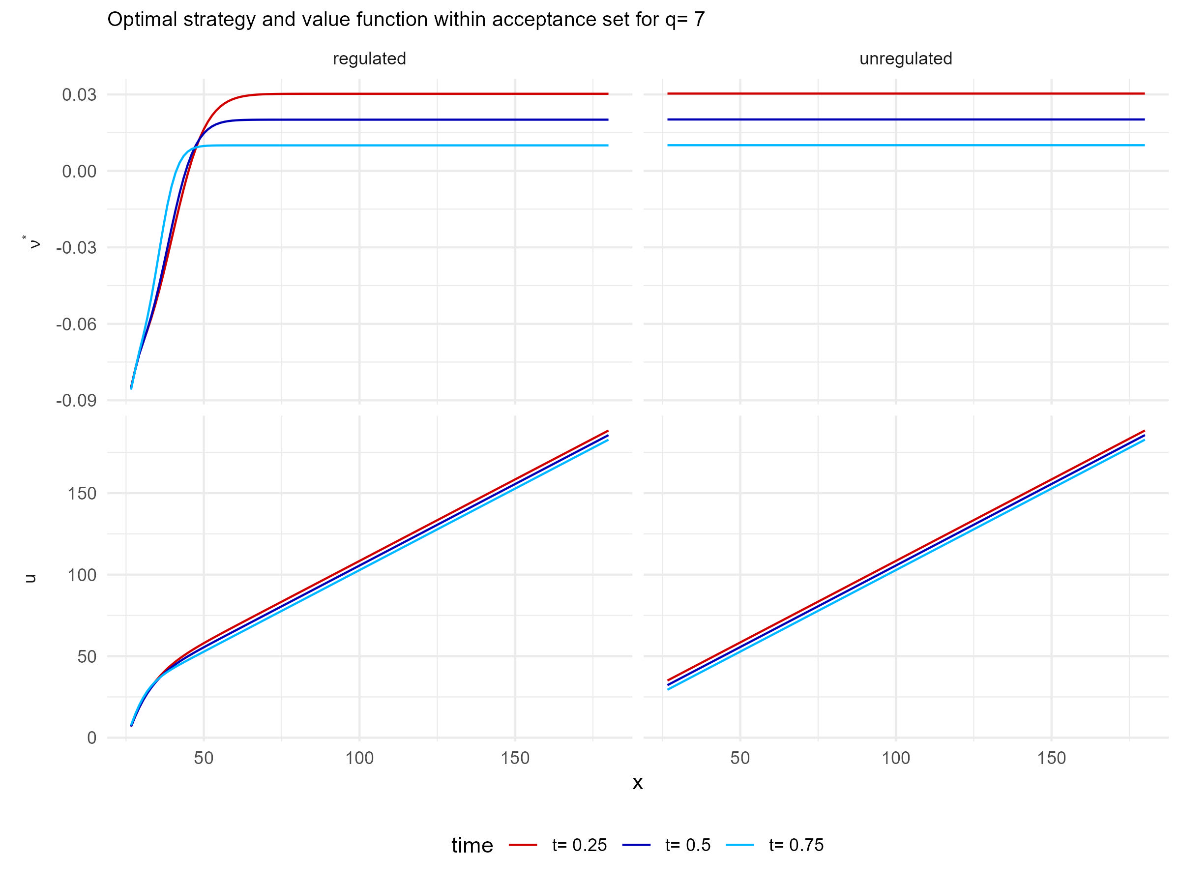
Figure 1. Graph of the optimal strategy (top) and of the value function (bottom) for fixed $q$ and several time points for $\mu_{\text{ex}}=1.6$. Left the case with boundary conditions; right the unregulated case. Parameters as in Scenario 1 of Table 1.

In Figure 2 we plot sections of the optimal strategy $\nu^{*}(t,\cdot,x)$ and of the value function value function $u(t,\cdot,x)$ for varying $q$ and fixed $x=32$ for various $t$, again for $\mu_{\text{ex}}=1.6$. If $q$ is far away from the liquidation boundary, strategy and value function coincide in the regulated and in the unregulated case. We see that $q$ close to the liquidation boundary banks are deleveraging to avoid liquidation. Moreover, for $q$ close to the boundary the value function is decreasing in $q$ whereas in the case without capital constraints it is increasing throughout (since in that case a higher inventory level means higher expected profits as $\mu_{\text{ex}}>0$.

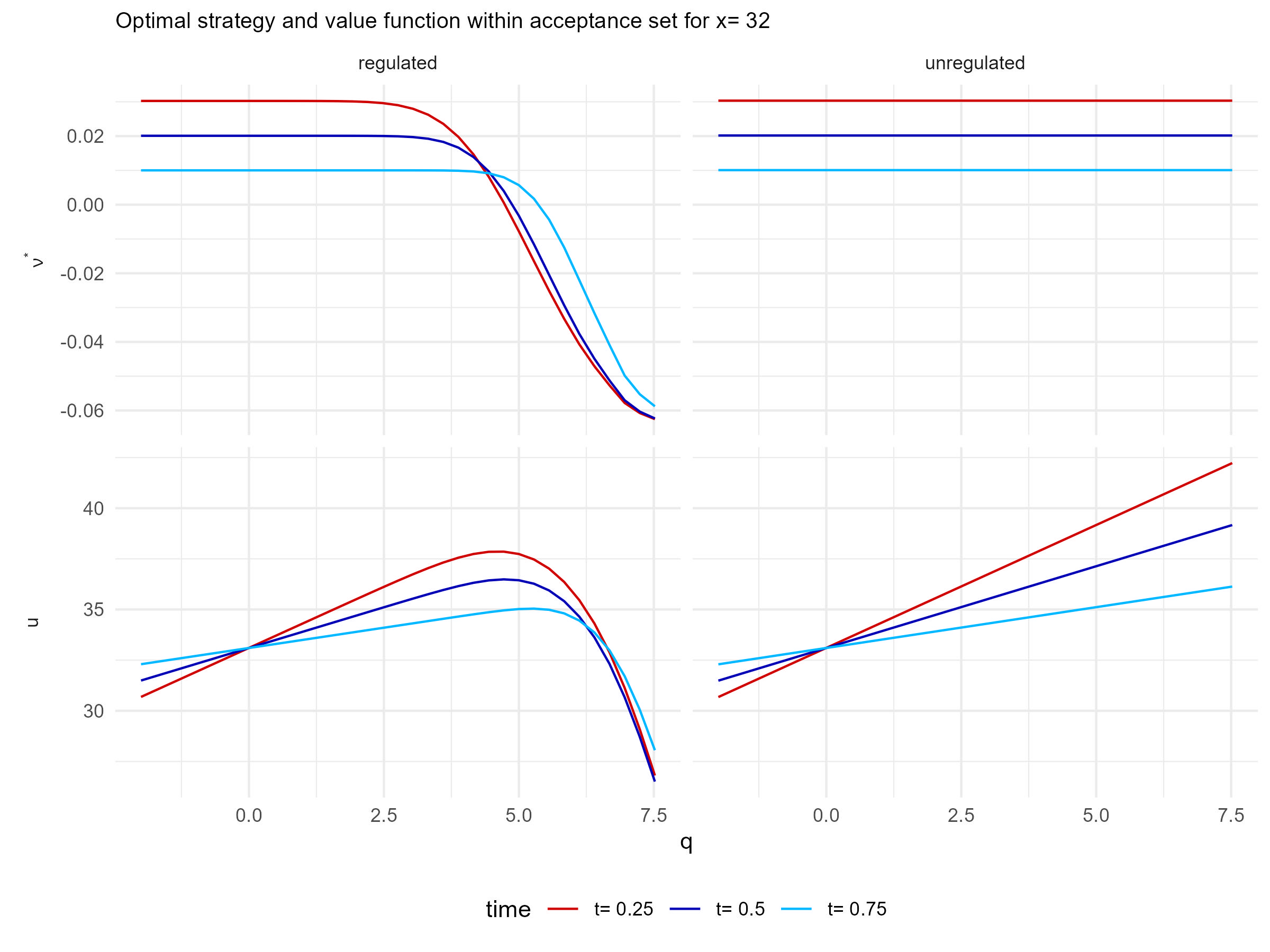
Figure 2. Graph of the optimal strategy (top) and of the value function (bottom) for fixed $x$ and several time points for $\mu_{\text{ex}}=1.6$. Left the case with boundary conditions; right the unregulated case. Parameters as in Scenario 1 of Table 1.

5.2. Stability of the banking system

Next we study the impact of capital constraints on the stability of the banking system. The parameters used are given in scenario 2 of Table 1. This parameter setting corresponding to a recession scenario where the assets of all banks trend downward ($\mu_{\text{ex}}=-1.6$) and where at $t=0$ a large fraction of the banking system is close to the liquidation boundary, due to the low value for the mean of the initial distribution of banks’ equity ($\mathbb{E}(X_{0})=60$). Note that the value for $\kappa$ is quite large so that that the trading rate is low; this corresponds to the case where the tradable asset is relatively illiquid.

Figure 3 shows contour plots of the density $m(t,q,x)$ at $t=0$ and $t=T$. Due to the negative drift $\mu_{\text{ex}}=-1.6$ the density curve is transported to the left over time (the average equity value decreases), as we would expect in a recession scenario. We observe that in the unregulated case this move is more pronounced.

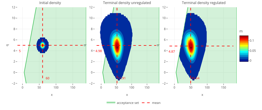
Figure 3. Contour plot of the population density (mean field) at $t=0$ and at $t=T$ for the unregulated case (left) and the regulated case (right); acceptance region $\mathcal{A}$ in green, parameters as in Scenario 2 of Table 1.

Figure 4 presents a summary of the evolution of the banking system. We observe that there is a strong spike in the liquidation intensity (the change in the proportion of liquidated banks per unit of time) and a strong decrease in $\overline{\mu}_{t}$ at $t\approx 0.9$, that is the system is close to a systemic crisis. In fact, if we increase the parameter $\alpha$, the Picard iterations cease to converge. Further, the plots show that in the regulated case the risk bearing capacity of the banking system (the average number of risky assets held by the system) and the mean book value of equity is lower than in the case with capital constraints.

Figure 4. Summary of the banking system in a recession scenario. Parameters as in Scenario 2 of Table 1. Note in particular the spike in the liquidation intensity at $t=0.9$.

5.3. Macroprudential policy measures

Finally, we analyze the impact of two macroprudential policy measures.

5.3.1. Increasing capitalization.

It is often argued that sufficient amount of equity capital in the banking system helps to stabilize the system, see for instance Admati and Hellwig [3] or Hanson et al. [21]. We therefore study how a higher level of initial equity affects the initial distribution of the system. In Figure 5 we plot the banking system for the same parameters as in Figure 4 except that we now assume that the mean of the initial equity distribution is $\mathbb{E}(X_{0})=70$ (scenario 3 of Table 1) and thus substantially higher than in Figure 4. We observe that the behaviour of the system is very similar to the unregulated case, in particular the spike in the liquidation intensity at $t=0.9$ has almost disappeared. This clearly supports regulatory efforts to ensure that banking systems are well capitalized.

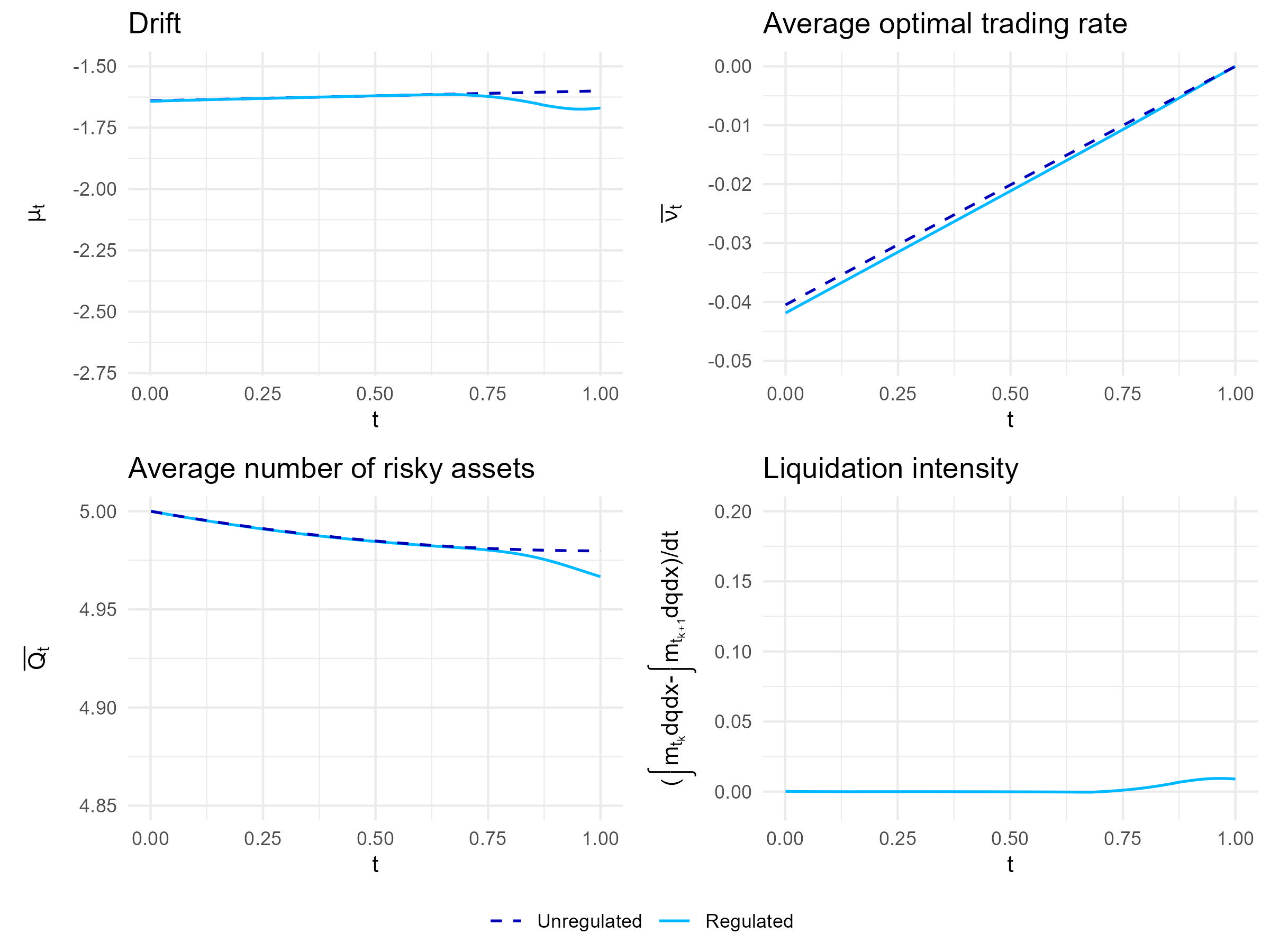
Figure 5. Summary of the banking system with higher initial capital ($\mathbb{E}[X_{0}]=70$), other parameters as in Figure 4. Parameters as in Scenario 3 of Table 1.

Improving the resolution mechanism.

The relatively low values for the average trading rate suggest that a systemic risk event is mostly due to the automatic and immediate liquidation of banks upon violation of the capital constraints and less due to the trading behavior of the active banks. This suggests that financial stability is enhanced if banks violating the capital constraints are resolved in a way that mitigates price-mediated contagion, for instance by parking the assets of these banks in a special purpose vehicle that is unwound only gradually over time. A simple way to test this conjecture in our framework is to work with a coefficient $\alpha_{\text{active}}$ for the impact of the trading of active banks and with a smaller coefficient $\alpha_{\text{liq}}$ for the impact of the liquidation. In Figure 6 we let $\alpha_{\text{active}}=0.8$ and $\alpha_{\text{liq}}=0.2$ (scenario 4 of Table 1). Figure  6 shows the corresponding liquidation intensity.

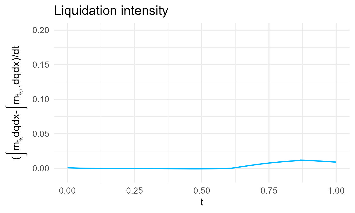
Figure 6. Liquidation intensity with smaller liquidation impact parameter $\alpha_{\text{liq}}$. Parameters are given in Scenario 4 of Table 1.

6. Conclusion

In this paper we have studied the impact of regulatory capital constraints on fire sales and financial stability in a large banking system using a mean field game of control (MFGC) model. In our setting banks adjust their holdings of a risky asset via trading strategies with finite trading rate. Moreover, a bank is liquidated if it violates a stylized regulatory capital constraint. We assumed that the drift of the asset value is affected by the average change in the position of the banks in the system, which creates price mediated contagion. Numerical methods were used to study properties of the banking system. We found that for high enough values of the contagion parameter a banking system that is not very well capitalized may experience a liquidation cascade or systemic risk event, where many banks default more or less simultaneously. These findings lends formal support to the conjecture from the regulatory literature that risk capital constraints may cause price-mediated contagion. They also support calls for macroprudential approaches to bank regulation (essentially regulatory efforts trying to mitigate the external effects of rapid deleveraging, see Hanson et al. [21]) in addition to standard capital constraints. Most importantly, regulators should ensure that the banking system is sufficiently well capitalized, as in that case the occurrence of a liquidation cascade is very unlikely. Moreover, it might help to consider improved resolution mechanisms for banks that violate the capital constraints and to park their assets in a special purpose vehicle that is unwound gradually over time.

Acknowledgements

We would like to thank Yves Achdou for his helpful comments regarding the numerical solution of our PDE system.

Appendix A Details on the numerical implementation

A.1. Overview and Notation

Our goal is to numerically solve the coupled PDE system (4.4) by first discretizing it and then using Picard iterations, where the value function and density describing the system are updated until convergence. The main challenges in solving the system numerically are (i) the coupling between the HJB and the forward equation, (ii) the fact that the HJB equation goes backward in time while the PDE describing the evolution of the density goes forward in time, (iii) the natural requirement for the density to be nonnegative and mass-preserving, and (iv) the nonlinearity of our system with respect to various partial derivatives. One common approach from literature to overcome the first three challenges is to use a special finite difference scheme consisting of a combination of right- and left-sided differences combined with Picard iterations until convergence of the system. We will shortly describe how we tackle the last challenge mentioned that arises from the structure of our PDE system. For completeness, let us start by introducing some standard notation needed for the discretization of the system.

For positive integers $N_{T},N_{Q}$,$N_{X}$, we define the time step size as $\Delta t=\frac{T}{N_{T}}$ and the step sized related to the state variables $Q$ and $X$ as $\Delta q=\frac{Q_{\text{max}}-Q_{\text{min}}}{N_{Q}}$ and $\Delta x=\frac{X_{\text{max}}-X_{\text{min}}}{N_{X}}$, respectively. The set of discrete time steps on our grid is then $\mathfrak{T}=\{t_{k}=k\Delta t,k=0,\dots,N_{T}\}$ and the grid corresponding to the state variable is $\mathfrak{H}=\{h_{ij}=(q_{i},x_{j})=(Q_{\text{min}}+i\Delta q,X_{\text{min}}+j\Delta x),i=0,\dots,N_{Q},j=0,\dots,N_{X}\}$. We aim to approximate $u(t_{k},h_{i,j})$ and $m(t_{k},h_{i,j})$ by $u_{i,j}^{k}$ and $m_{i,j}^{k}$, through solving the discrete approximations of the coupled PDE system. We define the following finite difference operators for some function $y:\mathfrak{T}\times\mathfrak{H}\to\mathbb{R}$

$$D_{t}y_{i,j}^{k}=\frac{y_{i,j}^{k+1}-y_{i,j}^{k}}{\Delta t},$$ [Discrete time derivative]

$$D_{q}y_{i,j}^{k}=\frac{y_{i+1,j}^{k}-y_{i-1,j}^{k}}{2\Delta q}, q$$ [Central difference operator in ]

$$D_{q}^{R}y_{i,j}^{k}=\frac{y_{i+1,j}^{k}-y_{i,j}^{k}}{\Delta q}, q$$ [Right difference operator in ]

$$D_{q}^{L}y_{i,j}^{k}=\frac{y_{i,j}^{k}-y_{i-1,j}^{k}}{\Delta q}, q$$ [Left difference operator in ]

$$D_{x}y_{i,j}^{k}=\frac{y_{i,j+1}^{k}-y_{i,j-1}^{k}}{2\Delta x}, x$$ [Central difference operator in ]

$$\Delta_{q}y_{i}^{k}=-\frac{1}{{\Delta q}^{2}}\left(2y_{i,j}^{k}-y_{i+1,j}^{k}-y_{i-1,j}^{k}\right), q$$ [Central second order difference in ]

$$\Delta_{x}y_{i,j}^{k}=-\frac{1}{{\Delta x}^{2}}\left(2y_{i,j}^{k}-y_{i,j+1}^{k}-y_{i,j-1}^{k}\right), x$$ [Central second order difference in ]

$$\Delta_{qx}y_{i,j}^{k}=\frac{D_{q}y_{i,j+1}^{k}-D_{q}y_{i,j-1}^{k}}{2\Delta x}$$

$$=\frac{y_{i+1,j+1}^{k}-y_{i-1,j+1}^{k}-y_{i+1,j-1}^{k}+y_{i-1,j-1}^{k}}{\Delta q\Delta x}.$$ [Mixed second order difference]

By definition of these operators, at boundary nodes the grid needs to be extended by one layer. We extend both the value function and the density linearly, i.e. by assuming $u(q+\Delta q,x)=u(q,x)+(u(q,x)-u(q-\Delta q,x))$, $u(q,x+\Delta x)=u(q,x)+(u(q,x)-u(q,x-\Delta x))$, and $m$ similarly. Before descritizing our equation system, we also need to rewrite some terms. Note that

$$\partial_{q}\left(\frac{\partial_{q}u}{2\kappa\partial_{x}u}m\right)=\partial_{q}\left(\frac{\partial_{q}u}{2\kappa\partial_{x}u}\right)m+\frac{\partial_{q}u}{2\kappa\partial_{x}u}\partial_{q}m=\frac{1}{2\kappa}\frac{\partial_{q}^{2}u\partial_{x}u-\partial_{q}u\partial_{q}\partial_{x}u}{\left(\partial_{x}u\right)^{2}}m+\frac{\partial_{q}u}{2\kappa\partial_{x}u}\partial_{q}m$$

and

$$\partial_{x}\left(\left(q(\mu_{\text{ex}}+\alpha\mu)-\frac{(\partial_{q}u)^{2}}{4\kappa(\partial_{x}u)^{2}}\right)m\right)=q(\mu_{\text{ex}}+\alpha\mu)\partial_{x}m-\partial_{x}\left(\frac{(\partial_{q}u)^{2}}{4\kappa(\partial_{x}u)^{2}}\right)m-\frac{(\partial_{q}u)^{2}}{4\kappa(\partial_{x}u)^{2}}\partial_{x}m$$

$$=q(\mu_{\text{ex}}+\alpha\mu)\partial_{x}m-\frac{1}{4\kappa}\frac{\partial_{x}(\partial_{q}u)^{2}\cdot(\partial_{x}u)^{2}-(\partial_{q}u)^{2}\cdot\partial_{x}(\partial_{x}u)^{2}}{(\partial_{x}u)^{4}}m-\frac{(\partial_{q}u)^{2}}{4\kappa(\partial_{x}u)^{2}}\partial_{x}m$$

$$=q(\mu_{\text{ex}}+\alpha\mu)\partial_{x}m-\frac{1}{4\kappa}\frac{2\partial_{q}u\partial_{x}\partial_{q}u\cdot(\partial_{x}u)^{2}-(\partial_{q}u)^{2}\cdot 2\partial_{x}u\partial_{x}^{2}u}{(\partial_{x}u)^{4}}m-\frac{(\partial_{q}u)^{2}}{4\kappa(\partial_{x}u)^{2}}\partial_{x}m.$$

A.2. Discretization

In what follows, with regards to the discretization of the system, we follow the idea proposed by Achdou and Laurière [2], who use a mix of right- and left-sided difference operators for the discretization in order to be able to overcome the mentioned challenges (i)-(iii). A numerical Hamiltonian is used that is non-increasing in the right-sided differences and non-decreasing in the left-sided differences of the state variable.

However, we need to modify this idea due to the complexity of our model. In our PDE system, there are terms whose monotonicity with respect to derivatives in different dimension is not clear, as they depend on derivatives with respect to both $q$ and $x$. We therefore use central difference operators in $x$, but distinguish between left- and right-sided difference operators in the dimension of $q$ in order to overcome challenge (iv). Thereby we can achieve better stability of our algorithm. Specifically, we choose the numerical Hamiltonian such that it is non-increasing in the right-sided difference $D_{q}^{R}$ and non-decreasing in the left-sided difference $D_{q}^{L}$.
We discretize the term $\frac{(\partial_{q}u)^{2}}{4\kappa\partial_{x}u}$ in the HJB as

$$\max\left\{\frac{\left[\left(D_{q}^{R}u_{i,j}^{k}\right)^{-}\right]^{2}}{4\kappa D_{x}u_{i,j}^{k}},\frac{\left[\left(D_{q}^{L}u_{i,j}^{k}\right)^{+}\right]^{2}}{4\kappa D_{x}u_{i,j}^{k}}\right\}.$$

For the forward equation, we discretize the term

$$\partial_{q}\left(\frac{\partial_{q}u}{2\kappa\partial_{x}u}m\right)=\frac{1}{2\kappa}\frac{\partial_{q}^{2}u\partial_{x}u-\partial_{q}u\partial_{q}\partial_{x}u}{\left(\partial_{x}u\right)^{2}}m+\frac{\partial_{q}u}{2\kappa\partial_{x}u}\partial_{q}m$$

as
$\frac{1}{2\kappa}\frac{\Delta_{q}u_{i,j}^{k}D_{x}u_{i,j}^{k}-\left\{\max\left[\left(D_{q}^{R}u_{i,j}^{k}\right)^{+}\left(\Delta_{qx}u_{i,j}^{k}\right)^{+},\left(D_{q}^{L}u_{i,j}^{k}\right)^{-}\left(\Delta_{qx}u_{i,j}^{k}\right)^{-}\right]+\min\left[\left(D_{q}^{R}u_{i,j}^{k}\right)^{-}\left(\Delta_{qx}u_{i,j}^{k}\right)^{+},\left(D_{q}^{L}u_{i,j}^{k}\right)^{+}\left(\Delta_{qx}u_{i,j}^{k}\right)^{-}\right]\right\}}{\left(D_{x}u_{i,j}^{k}\right)^{2}}m_{i,j}^{k}$ $+\frac{1}{2\kappa D_{x}u_{i,j}^{k}}\Bigg{[}\max\left\{(D_{q}^{L}u_{i,j}^{k})^{+}(D_{q}^{L}m_{i,j}^{k})^{+},(D_{q}^{R}u_{i,j}^{k})^{-}(D_{q}^{R}m_{i,j}^{k})^{-}\right\}$
$+\min\left\{(D_{q}^{R}u_{i,j}^{k})^{+}(D_{q}^{L}m_{i,j}^{k})^{-},(D_{q}^{L}u_{i,j}^{k})^{-}(D_{q}^{R}m_{i,j}^{k})^{+}\right\}\Bigg{]}$ ,
and the term

$$\partial_{x}\left(\left(q(\mu_{\text{ex}}+\alpha\mu)-\frac{(\partial_{q}u)^{2}}{4\kappa(\partial_{x}u)^{2}}\right)m\right)$$

$$=q(\mu_{\text{ex}}+\alpha\mu)\partial_{x}m-\frac{1}{4\kappa}\frac{2\partial_{q}u\partial_{x}\partial_{q}u\cdot(\partial_{x}u)^{2}-(\partial_{q}u)^{2}\cdot 2\partial_{x}u\partial_{x}^{2}u}{(\partial_{x}u)^{4}}m-\frac{(\partial_{q}u)^{2}}{4\kappa(\partial_{x}u)^{2}}\partial_{x}m,$$

as
$q(\mu_{ex}+\alpha\mu^{k}+\delta)D_{x}m_{i,j}^{k}$
$-\frac{1}{4\kappa}\frac{2\left(D_{x}u_{i,j}^{k}\right)^{2}\cdot\left\{\max\left[\left(D_{q}^{L}u_{i,j}^{k}\right)^{+}\left(\Delta_{qx}u_{i,j}^{k}\right)^{+},\left(D_{q}^{R}u_{i,j}^{k}\right)^{-}\left(\Delta_{qx}u_{i,j}^{k}\right)^{-}\right]+\min\left[\left(D_{q}^{L}u_{i,j}^{k}\right)^{-}\left(\Delta_{qx}u_{i,j}^{k}\right)^{+},\left(D_{q}^{R}u_{i,j}^{k}\right)^{+}\left(\Delta_{qx}u_{i,j}^{k}\right)^{-}\right]\right\}}{(D_{x}u_{i,j}^{k})^{4}}m_{i,j}^{k}$
$+\frac{1}{4\kappa}\frac{\max\left\{\left[\left(D_{q}^{R}u_{i,j}^{k}\right)^{-}\right]^{2},\left[\left(D_{q}^{L}u_{i,j}^{k}\right)^{+}\right]^{2}\right\}\cdot 2D_{x}u_{i,j}^{k}\Delta_{x}u_{i,j}^{k}}{(D_{x}u_{i,j}^{k})^{4}}m_{i,j}^{k}$ $-\max\left\{\frac{\left[\left(D_{q}^{L}u_{i,j}^{k}\right)^{-}\right]^{2}}{4\kappa\left(D_{x}u_{i,j}^{k}\right)^{2}},\frac{\left[\left(D_{q}^{R}u_{i,j}^{k}\right)^{+}\right]^{2}}{4\kappa\left(D_{x}u_{i,j}^{k}\right)^{2}}\right\}D_{x}m_{i,j}^{k}$. To shorten the notation we define

$$F_{ij}(u^{k},m^{k}):=\frac{1}{2\kappa}\Bigg{(}\frac{\Delta_{q}u_{i,j}^{k}D_{x}u_{i,j}^{k}}{\left(D_{x}u_{i,j}^{k}\right)^{2}}$$

$$\,-\frac{\max\left[\left(D_{q}^{R}u_{i,j}^{k}\right)^{+}\left(\Delta_{qx}u_{i,j}^{k}\right)^{+},\left(D_{q}^{L}u_{i,j}^{k}\right)^{-}\left(\Delta_{qx}u_{i,j}^{k}\right)^{-}\right]+\min\left[\left(D_{q}^{R}u_{i,j}^{k}\right)^{-}\left(\Delta_{qx}u_{i,j}^{k}\right)^{+},\left(D_{q}^{L}u_{i,j}^{k}\right)^{+}\left(\Delta_{qx}u_{i,j}^{k}\right)^{-}\right]}{\left(D_{x}u_{i,j}^{k}\right)^{2}}\Bigg{)}m_{i,j}^{k}$$

$$\,+\frac{1}{2\kappa D_{x}u_{i,j}^{k}}\Big{[}\max\left\{(D_{q}^{L}u_{i,j}^{k})^{+}(D_{q}^{L}m_{i,j}^{k})^{+},(D_{q}^{R}u_{i,j}^{k})^{-}(D_{q}^{R}m_{i,j}^{k})^{-}\right\}$$

$$\,+\min\left\{(D_{q}^{R}u_{i,j}^{k})^{+}(D_{q}^{L}m_{i,j}^{k})^{-},(D_{q}^{L}u_{i,j}^{k})^{-}(D_{q}^{R}m_{i,j}^{k})^{+}\right\}\Big{]}+q(\mu_{ex}+\alpha\mu^{k}+\delta)D_{x}m_{i,j}^{k}$$

$$\,-\frac{2\left(D_{x}u_{i,j}^{k}\right)^{2}\cdot\left\{\max\left[\left(D_{q}^{L}u_{i,j}^{k}\right)^{+}\left(\Delta_{qx}u_{i,j}^{k}\right)^{+},\left(D_{q}^{R}u_{i,j}^{k}\right)^{-}\left(\Delta_{qx}u_{i,j}^{k}\right)^{-}\right]+\min\left[\left(D_{q}^{L}u_{i,j}^{k}\right)^{-}\left(\Delta_{qx}u_{i,j}^{k}\right)^{+},\left(D_{q}^{R}u_{i,j}^{k}\right)^{+}\left(\Delta_{qx}u_{i,j}^{k}\right)^{-}\right]\right\}}{4\kappa(D_{x}u_{i,j}^{k})^{4}}m_{i,j}^{k}$$

$$\,+\frac{\max\left\{\left[\left(D_{q}^{R}u_{i,j}^{k}\right)^{-}\right]^{2},\left[\left(D_{q}^{L}u_{i,j}^{k}\right)^{+}\right]^{2}\right\}\cdot 2D_{x}u_{i,j}^{k}\Delta_{x}u_{i,j}^{k}}{4\kappa(D_{x}u_{i,j}^{k})^{4}}m_{i,j}^{k}-\max\left\{\frac{\left[\left(D_{q}^{L}u_{i,j}^{k}\right)^{-}\right]^{2}}{4\kappa\left(D_{x}u_{i,j}^{k}\right)^{2}},\frac{\left[\left(D_{q}^{R}u_{i,j}^{k}\right)^{+}\right]^{2}}{4\kappa\left(D_{x}u_{i,j}^{k}\right)^{2}}\right\}D_{x}m_{i,j}^{k},$$

which leads to the following discretized PDE system.

$$\begin{cases}D_{t}u_{i,j}^{k}+q_{i}(\mu_{\text{ex}}+\alpha\mu^{k})D_{x}u_{i,j}^{k}+\frac{1}{2}\sigma_{Q}^{2}\Delta_{q}u_{i,j}^{k}+\frac{1}{2}\left(\sigma_{A}^{2}+\sigma_{S}^{2}q_{i}^{2}\right)\Delta_{x}u^{k}_{i,j}\\ +\max\left\{\frac{\left[\left(D_{q}^{R}u_{i,j}^{k}\right)^{-}\right]^{2}}{4\kappa D_{x}u_{i,j}^{k}},\frac{\left[\left(D_{q}^{L}u_{i,j}^{k}\right)^{+}\right]^{2}}{4\kappa D_{x}u_{i,j}^{k}}\right\}=0,\\ D_{t}m_{i,j}^{k}-\frac{1}{2}\sigma_{Q}^{2}\Delta_{q}m_{i,j}^{k}-\frac{1}{2}\left(\sigma_{A}^{2}+\sigma_{S}^{2}q^{2}\right)\Delta_{x}m_{i,j}^{k}+F_{i,j}(u^{k},m^{k})=0\\ \mu^{k}=D_{t}\left(\sum_{i}\sum_{j}q_{i}m_{i,j}^{k}\Delta x\Delta q\right),\\ u(T,q_{i},x_{j})=x_{j}-\gamma q_{i}^{2},\\ m(0,q_{i},x_{j})=m_{0}(x_{i},q_{j}),\\ u(t_{k},q_{i},x_{j})\equiv k(t_{k})\cdot(\beta q_{i}+c)\text{ on }\mathcal{A}^{c},\\ m(t_{k},q_{i},x_{j})\equiv 0\text{ on }\mathcal{A}^{c}.\end{cases}$$

A.3. Picard Iteration

The discretized PDE system can now be used to update initial guesses of the value function $u$ (backward in time) and the density $m$ (forward in time) iteratively, until a convergence criterion is met.

We implement these Picard iterations in R. The following pseudo code shows the structure of the algorithm.

Iterative Solvers
function $\mathtt{iterate_{u}(u,m)}$					iteration of u
	for $k=N_{T}-1,\dots,1$				backward iteration
		$l=0$
		$u^{0}=u$
		$\mu^{k}=D_{t}\left(\sum_{i}\sum_{j}q_{i}m_{i,j}^{k}\Delta x\Delta q\right)$			drift
		while error $>$ tolerance
			$l=l+1$		iteration step
			$u_{ij}^{k,l}=u_{ij}^{k+1,l}+\Delta t\cdot\Bigg{[}q_{i}(\mu_{\text{ex}}+\alpha\mu^{k})D_{x}u_{i,j}^{k,l}+\frac{1}{2}\sigma_{Q}^{2}\Delta_{q}u_{i,j}^{k,l}$		updated value function
				$+\frac{1}{2}\left(\sigma_{A}^{2}+\sigma_{S}^{2}q_{i}^{2}\right)\Delta_{x}u^{k,l}_{i,j}+\max\left\{\frac{\left[\left(D_{q}^{R}u_{i,j}^{k,l}\right)^{-}\right]^{2}}{4\kappa D_{x}u_{i,j}^{k,l}},\frac{\left[\left(D_{q}^{L}u_{i,j}^{k,l}\right)^{+}\right]^{2}}{4\kappa D_{x}u_{i,j}^{k,l}}\right\}\Bigg{]}$
			if $\text{regulated}=\texttt{TRUE}$  $u_{ij}^{k,l}[\mathcal{A}^{c}]=k(t_{k})\cdot(\beta q_{i}+c)$		boundary condition
			$\text{error}=\text{mean}(\text{abs}(u_{ij}^{k,l}-u_{ij}^{k,l-1}))$		error between guesses
return $u$
function $\mathtt{iterate_{m}(u,m)}$					iteration of m
	for $k=1,\dots,N_{T}-1$				forward iteration
		$p=0$
		$m^{0}=m$
		while error $>$ tolerance
			$\mu^{k,p}=D_{t}\left(\sum_{i}\sum_{j}q_{i}m_{i,j}^{k,p}\Delta x\Delta q\right)$		drift
			$p=p+1$		iteration step
			$m_{ij}^{k+1,p}=m_{ij}^{k,p}-\Delta t\Big{[}-\frac{1}{2}\sigma_{Q}^{2}\Delta_{q}m_{i,j}^{k,p}-\frac{1}{2}\left(\sigma_{A}^{2}+\sigma_{S}^{2}q^{2}\right)\Delta_{x}m_{i,j}^{k,p}+F_{ij}(u^{k,p},m^{k,p})\Big{]}$		updated density
			if $\text{regulated}=\texttt{TRUE}$  $m_{ij}^{k+1,p}[\mathcal{A}^{c}]=0$		boundary condition
			$\text{error}=\text{mean}(\text{abs}(m_{ij}^{k+1,p}-m_{ij}^{k+1,p-1}))$		error between guesses
return $m$
Picard Iteration
$u=u_{T}$, $m=m_{0}$					initialization
$n=0$					iteration step
while error $>$ tolerance					iteration on whole grid
	$n=n+1$				iteration step
	$u=\mathtt{iterate_{u}(u,m)}$				iteration of u
	$m=\mathtt{iterate_{m}(u,m)}$				iteration of m
	$\text{error}=\Big{[}\text{mean}(\text{abs}(u_{ij}^{k,n}-u_{ij}^{k,n-1}))+\text{mean}(\text{abs}(m_{ij}^{k,n}-m_{ij}^{k,n-1}))\Big{]}/2$				error between guesses

Appendix B Details on the explicit solution in the unregulated case

In this section we give explicit expressions for the functions $h_{0}$ and $h_{1}$ that arise in the explicit solution for the MFGC in the unconstrained case. We get for $h_{1}$

$$h_{1} =2\kappa E^{\prime}+h_{2}E$$

$$=2\kappa\left[\frac{\left(\mu_{\text{ex}}\alpha+\frac{\alpha\mu_{\text{ex}}\gamma}{\kappa}T-E_{0}\frac{\alpha^{2}\gamma}{\kappa}\right)e^{-\frac{\alpha}{2\kappa}t}}{\left(\alpha^{2}-2\gamma\alpha\right)e^{-\frac{\alpha}{2\kappa}T}+2\gamma\alpha}-\frac{\mu_{\text{ex}}}{\alpha}\right]$$

$$+\frac{2\kappa}{T-t+\frac{\kappa}{\gamma}}\left[\frac{E_{0}\left(\alpha^{2}e^{-\frac{\alpha}{2\kappa}T}+2\gamma\alpha\left(e^{-\frac{\alpha}{2\kappa}t}-e^{-\frac{\alpha}{2\kappa}T}\right)\right)-\left(2\kappa\mu_{\text{ex}}+2\mu_{\text{ex}}\gamma T\right)\left(e^{-\frac{\alpha}{2\kappa}t}-1\right)}{\left(\alpha^{2}-2\gamma\alpha\right)e^{-\frac{\alpha}{2\kappa}T}+2\gamma\alpha}-\frac{\mu_{\text{ex}}}{\alpha}t\right].$$

Given $h_{1}$, we can compute $h_{0}$ using (3.6b),

$$h_{0}^{\prime} =-\frac{h_{1}^{2}}{4\kappa}=-\frac{4\kappa^{2}E^{\prime 2}+4\kappa h_{2}EE^{\prime}+h_{2}^{2}E^{2}}{4\kappa}=-\kappa E^{\prime 2}-\frac{2\kappa}{T-t+\frac{\kappa}{\gamma}}EE^{\prime}-\frac{\kappa}{(T-t+\frac{\kappa}{\gamma})^{2}}E^{2}$$

$$=-\kappa\left[\frac{\left(\mu_{\text{ex}}\alpha+\frac{\alpha\mu_{\text{ex}}\gamma}{\kappa}T-E_{0}\frac{\alpha^{2}\gamma}{\kappa}\right)e^{-\frac{\alpha}{2\kappa}t}}{\left(\alpha^{2}-2\gamma\alpha\right)e^{-\frac{\alpha}{2\kappa}T}+2\gamma\alpha}-\frac{\mu_{\text{ex}}}{\alpha}\right]^{2}$$

$$-\frac{2\kappa}{T-t+\frac{\kappa}{\gamma}}\left[\frac{E_{0}\left(\alpha^{2}e^{-\frac{\alpha}{2\kappa}T}+2\gamma\alpha\left(e^{-\frac{\alpha}{2\kappa}t}-e^{-\frac{\alpha}{2\kappa}T}\right)\right)-\left(2\kappa\mu_{\text{ex}}+2\mu_{\text{ex}}\gamma T\right)\left(e^{-\frac{\alpha}{2\kappa}t}-1\right)}{\left(\alpha^{2}-2\gamma\alpha\right)e^{-\frac{\alpha}{2\kappa}T}+2\gamma\alpha}-\frac{\mu_{\text{ex}}}{\alpha}t\right]$$

$$\cdot\left[\frac{\left(\mu_{\text{ex}}\alpha+\frac{\alpha\mu_{\text{ex}}\gamma}{\kappa}T-E_{0}\frac{\alpha^{2}\gamma}{\kappa}\right)e^{-\frac{\alpha}{2\kappa}t}}{\left(\alpha^{2}-2\gamma\alpha\right)e^{-\frac{\alpha}{2\kappa}T}+2\gamma\alpha}-\frac{\mu_{\text{ex}}}{\alpha}\right]$$

$$-\frac{\kappa}{(T-t+\frac{\kappa}{\gamma})^{2}}\left[\frac{E_{0}\left(\alpha^{2}e^{-\frac{\alpha}{2\kappa}T}+2\gamma\alpha\left(e^{-\frac{\alpha}{2\kappa}t}-e^{-\frac{\alpha}{2\kappa}T}\right)\right)-\left(2\kappa\mu_{\text{ex}}+2\mu_{\text{ex}}\gamma T\right)\left(e^{-\frac{\alpha}{2\kappa}t}-1\right)}{\left(\alpha^{2}-2\gamma\alpha\right)e^{-\frac{\alpha}{2\kappa}T}+2\gamma\alpha}-\frac{\mu_{\text{ex}}}{\alpha}t\right]^{2}$$

$$=:\Omega^{\prime}+\Gamma^{\prime}+\Pi^{\prime}.$$

For $h_{0}$ we obtain

$$h_{0}=\Omega+\Gamma+\Pi,$$

where

$$\Omega =-\frac{\kappa}{\alpha}\frac{\left(-\mu_{\text{ex}}^{2}\alpha^{2}\kappa-\frac{\alpha^{2}\mu_{\text{ex}}^{2}\gamma^{2}}{\kappa}T^{2}-E_{0}^{2}\frac{\alpha^{4}\gamma^{2}}{\kappa}-2\alpha^{2}\mu_{\text{ex}}^{2}\gamma T+2E_{0}\alpha^{3}\mu_{\text{ex}}\gamma+2\frac{\alpha^{3}\mu_{\text{ex}}\gamma^{2}}{\kappa}TE_{0}\right)e^{-\frac{\alpha}{\kappa}t}}{\left(\left(\alpha^{2}-2\gamma\alpha\right)e^{-\frac{\alpha}{2\kappa}T}+2\gamma\alpha\right)^{2}}$$

$$-2\frac{2\kappa}{\alpha}\frac{\left(\mu_{\text{ex}}^{2}\kappa+\mu_{\text{ex}}^{2}\gamma T-E_{0}\alpha\gamma\mu_{\text{ex}}\right)e^{-\frac{\alpha}{2\kappa}t}}{\left(\alpha^{2}-2\gamma\alpha\right)e^{-\frac{\alpha}{2\kappa}T}+2\gamma\alpha}-\frac{\mu_{\text{ex}}^{2}\kappa}{\alpha^{2}}t+C_{1}$$

$$=\frac{\left(\mu_{\text{ex}}^{2}\alpha\kappa^{2}+\alpha\mu_{\text{ex}}^{2}\gamma^{2}T^{2}+E_{0}^{2}\alpha^{3}\gamma^{2}+2\alpha\kappa\mu_{\text{ex}}^{2}\gamma T-2E_{0}\alpha^{2}\mu_{\text{ex}}\kappa\gamma-2\alpha^{2}\mu_{\text{ex}}\gamma^{2}TE_{0}\right)e^{-\frac{\alpha}{\kappa}t}}{\left(\left(\alpha^{2}-2\gamma\alpha\right)e^{-\frac{\alpha}{2\kappa}T}+2\gamma\alpha\right)^{2}}$$

$$-4\frac{\left(\frac{\mu_{\text{ex}}^{2}\kappa^{2}}{\alpha}+\frac{\mu_{\text{ex}}^{2}\kappa\gamma}{\alpha}T-E_{0}\kappa\gamma\mu_{\text{ex}}\right)e^{-\frac{\alpha}{2\kappa}t}}{\left(\alpha^{2}-2\gamma\alpha\right)e^{-\frac{\alpha}{2\kappa}T}+2\gamma\alpha}-\frac{\mu_{\text{ex}}^{2}\kappa}{\alpha^{2}}t+C_{1},$$

$$\Gamma =-\Bigg{[}\frac{\left(\left(4\gamma\alpha E_{0}-2\alpha^{2}E_{0}\right)e^{-\frac{\alpha}{2\kappa}T}-\left(4\kappa\mu_{\text{ex}}+4\mu_{\text{ex}}\gamma T\right)\right)\left(\mu_{\text{ex}}\alpha\kappa+\alpha\mu_{\text{ex}}\gamma T-E_{0}\alpha^{2}\gamma\right)}{\left(\left(\alpha^{2}-2\gamma\alpha\right)e^{-\frac{\alpha}{2\kappa}T}+2\gamma\alpha\right)^{2}}$$

$$+\frac{8E_{0}\gamma\mu_{\text{ex}}\kappa-\left(4\frac{\kappa^{2}\mu_{\text{ex}}^{2}}{\alpha}+4\frac{\mu_{\text{ex}}^{2}\gamma\kappa}{\alpha}T\right)}{\left(\alpha^{2}-2\gamma\alpha\right)e^{-\frac{\alpha}{2\kappa}T}+2\gamma\alpha}\Bigg{]}e^{-\frac{\alpha(\gamma T+\kappa)}{2\gamma\kappa}}\operatorname{Ei}\left(\frac{\alpha(\kappa+\gamma(T-t))}{2\gamma\kappa}\right)$$

$$-\frac{\left(4\kappa\mu_{\text{ex}}+4\mu_{\text{ex}}\gamma T-4\gamma\alpha E_{0}\right)\left(\mu_{\text{ex}}\alpha\kappa+\alpha\mu_{\text{ex}}\gamma T-E_{0}\alpha^{2}\gamma\right)}{\left(\left(\alpha^{2}-2\gamma\alpha\right)e^{-\frac{\alpha}{2\kappa}T}+2\gamma\alpha\right)^{2}}e^{-\frac{\alpha(\gamma T+\kappa)}{\gamma\kappa}}\operatorname{Ei}\left(\frac{\alpha(\kappa+\gamma(T-t))}{\gamma\kappa}\right)$$

$$-\frac{\left(2E_{0}\alpha\mu_{\text{ex}}\kappa-8E_{0}\gamma\mu_{\text{ex}}\kappa\right)e^{-\frac{\alpha}{2\kappa}T}+4\frac{\kappa^{2}\mu_{\text{ex}}^{2}}{\alpha}+4\frac{\mu_{\text{ex}}^{2}\gamma\kappa}{\alpha}T}{\left(\alpha^{2}-2\gamma\alpha\right)e^{-\frac{\alpha}{2\kappa}T}+2\gamma\alpha}\log\left(T-t+\frac{\kappa}{\gamma}\right)$$

$$+\frac{\left(2\mu_{\text{ex}}^{2}\kappa+2\mu_{\text{ex}}^{2}\gamma T-2E_{0}\alpha\mu_{\text{ex}}\gamma\right)}{\left(\alpha^{2}-2\gamma\alpha\right)e^{-\frac{\alpha}{2\kappa}T}+2\gamma\alpha}\frac{e^{-\frac{\alpha(\kappa+\gamma(T+t))}{2\gamma\kappa}}}{\alpha\gamma}\left[2\gamma\kappa e^{\frac{\alpha(\kappa+\gamma T)}{2\gamma\kappa}}-\alpha e^{\frac{\alpha t}{2\kappa}}(\gamma T+\kappa)\operatorname{Ei}\left(\frac{\alpha(\kappa+\gamma(T-t))}{2\gamma\kappa}\right)\right]$$

$$+\frac{2\kappa\mu_{\text{ex}}^{2}}{\alpha^{2}}\left(\frac{\gamma T+\kappa}{\gamma}\log\left(\gamma(T-t)+\kappa\right)+t\right)+C_{2},$$

and

$$\Pi =-\frac{\left(2E_{0}\gamma\alpha-2\kappa\mu_{\text{ex}}-2\mu_{\text{ex}}\gamma T\right)^{2}}{\left(\left(\alpha^{2}-2\gamma\alpha\right)e^{-\frac{\alpha}{2\kappa}T}+2\gamma\alpha\right)^{2}}\frac{e^{-\frac{\alpha(\gamma T+\kappa)}{\gamma\kappa}}\left(\gamma\kappa e^{\frac{\alpha(\gamma(T-t)+\kappa)}{\gamma\kappa}}-\alpha(\gamma(T-t)+\kappa)\operatorname{Ei}\left(\frac{\alpha(\gamma(T-t)+\kappa)}{\gamma\kappa}\right)\right)}{\gamma(T-t)+\kappa}$$

$$-\frac{\left(4E_{0}\gamma\alpha-4\kappa\mu_{\text{ex}}-4\mu_{\text{ex}}\gamma T\right)\left(E_{0}\alpha^{2}-2E_{0}\gamma\alpha\right)e^{-\frac{\alpha}{2\kappa}T}+\left(4E_{0}\gamma\alpha-4\kappa\mu_{\text{ex}}-4\mu_{\text{ex}}\gamma T\right)\left(2\kappa\mu_{\text{ex}}+2\mu_{\text{ex}}\gamma T\right)}{\left(\left(\alpha^{2}-2\gamma\alpha\right)e^{-\frac{\alpha}{2\kappa}T}+2\gamma\alpha\right)^{2}}$$

$$\cdot\frac{e^{-\frac{\alpha(\gamma T+\kappa)}{2\gamma\kappa}}\left(2\gamma\kappa e^{\frac{\alpha(\gamma(T-t)+\kappa)}{2\gamma\kappa}}-\alpha(\gamma(T-t)+\kappa)\operatorname{Ei}\left(\frac{\alpha(\gamma(T-t)+\kappa)}{2\gamma\kappa}\right)\right)}{2(\gamma(T-t)+\kappa)}$$

$$-\frac{\left(E_{0}\alpha^{2}-2E_{0}\gamma\alpha\right)^{2}e^{-\frac{\alpha}{\kappa}T}+\left(2\kappa\mu_{\text{ex}}+2\mu_{\text{ex}}\gamma T\right)^{2}+2\left(E_{0}\alpha^{2}-2E_{0}\gamma\alpha\right)e^{-\frac{\alpha}{2\kappa}T}\left(2\kappa\mu_{\text{ex}}+2\mu_{\text{ex}}\gamma T\right)}{\left(\left(\alpha^{2}-2\gamma\alpha\right)e^{-\frac{\alpha}{2\kappa}T}+2\gamma\alpha\right)^{2}}\frac{\kappa}{T-t+\frac{\kappa}{\gamma}}$$

$$+\frac{4E_{0}\gamma\mu_{\text{ex}}-\left(4\frac{\kappa\mu_{\text{ex}}^{2}}{\alpha}+4\frac{\mu_{\text{ex}}^{2}\gamma}{\alpha}T\right)}{\left(\alpha^{2}-2\gamma\alpha\right)e^{-\frac{\alpha}{2\kappa}T}+2\gamma\alpha}\frac{\kappa}{2\gamma\kappa(\gamma(T-t)+\kappa)}e^{-\frac{\alpha(\kappa+\gamma T)}{2\gamma\kappa}}$$

$$\cdot\left(-(\gamma(T-t)+\kappa)(\alpha\kappa-2\gamma\kappa+\gamma\alpha T)\operatorname{Ei}\left(\frac{\alpha(\kappa+\gamma(T-t))}{2\gamma\kappa}\right)+2\gamma\kappa(\kappa+\gamma T)e^{\frac{\alpha(\kappa+\gamma(T-t))}{2\gamma\kappa}}\right)$$

$$+\frac{2E_{0}\alpha\mu_{\text{ex}}e^{-\frac{\alpha}{2\kappa}T}-4E_{0}\gamma\mu_{\text{ex}}e^{-\frac{\alpha}{2\kappa}T}+\left(4\frac{\kappa\mu_{\text{ex}}^{2}}{\alpha}+4\frac{\mu_{\text{ex}}^{2}\gamma}{\alpha}T\right)}{\left(\alpha^{2}-2\gamma\alpha\right)e^{-\frac{\alpha}{2\kappa}T}+2\gamma\alpha}\frac{\kappa\left[(\gamma(T-t)+\kappa)\log\left(T-t+\frac{\kappa}{\gamma}\right)+\gamma T+\kappa\right]}{\gamma(T-t)+\kappa}$$

$$-\frac{\mu_{\text{ex}}^{2}\kappa}{\alpha^{2}}\left[\frac{(\gamma T+\kappa)^{2}}{\gamma^{2}\left(T-t+\frac{\kappa}{\gamma}\right)}+\frac{2(\gamma T+\kappa)\log\left(T-t+\frac{\kappa}{\gamma}\right)}{\gamma}+t\right]+C_{3}.$$

Note that it is determined only up to a constant $C:=C_{1}+C_{2}+C_{3}$. Recall that $h_{0}(T)=0$, from which we can determine the constant. $\operatorname{Ei}$ denotes the exponential integral.

References

• Achdou and Kobeissi [2021] Y. Achdou and Z. Kobeissi. Mean field games of controls: Finite difference approximations. Mathematics in Engineering, 3(3):1–35, 2021. doi: 10.3934/mine.2021024.
• Achdou and Laurière [2020] Yves Achdou and Mathieu Laurière. Mean field games and applications: Numerical aspects, 2020.
• Admati and Hellwig [2013] A. Admati and M. Hellwig. The Bankers’ New Clothes: What’s Wrong with Banking and What to Do about It. Princeton University Press, Princeton, NJ, 2013.
• Basel Committee on Banking Supervision [2014] Basel Committee on Banking Supervision. Basel III leverage ratio framework and disclosure requirements, January 2014. Bank of International Settlements.
• Braouezec and Wagalath [2019] Yann Braouezec and Lakshithe Wagalath. Strategic fire-sales and price-mediated contagion in the banking system. European Journal of Operational Research, 274(3):1180–1197, 2019. doi: https://doi.org/10.1016/j.ejor.2018.11.012.
• Cardaliaguet and LeHalle [2018] P. Cardaliaguet and C. A. LeHalle. Mean field game of controls and an application to trade crowding. Mathematics and Financial Economics, 12:335–363, 2018.
• Cardaliaguet and Porretta [2019] P. Cardaliaguet and A. Porretta, editors. Mean Field Games, Lecture Notes in Mathematics 2281, 2019. Cime, Springer.
• Carmona and Delarue [2018] René Carmona and François Delarue. Probabilistic Theory of Mean Field Games with Applications I-II. Springer International Publishing, 2018.
• Carmona et al. [2015] René Carmona, Jean-Pierre Fouque, and Li-Hsien Sun. Mean field games and systemic risk. Communications in Mathematical Sciences, 13(4):911 – 933, 2015. doi: 10.4310/CMS.2015.v13.n4.a4. Cited by: 96; All Open Access, Green Open Access.
• Cont and Wagalath [2016] R. Cont and L. Wagalath. Fire sales forensics: Measuring endogenous risk. Mathematical Finance, 26(4):835–866, 2016. doi: https://doi.org/10.1111/mafi.12071.
• Cont and Schaanning [2019] Rama Cont and Eric Schaanning. Monitoring indirect contagion. Journal of Banking and Finance, 104:85–102, 2019. doi: https://doi.org/10.1016/j.jbankfin.2019.04.007.
• Cuchiero et al. [2023] Christa Cuchiero, Stefan Rigger, and Sara Svaluto-Ferro. Propagation of minimality in the supercooled Stefan problem. The Annals of Applied Probability, 33(2):1588 – 1618, 2023. doi: 10.1214/22-AAP1850.
• Delarue et al. [2015] François Delarue, James Inglis, Sylvain Rubenthaler, and Etienne Tanré. Global solvability of a networked integrate-and-fire model of McKean–Vlasov type. The Annals of Applied Probability, 25(4):2096 – 2133, 2015. doi: 10.1214/14-AAP1044.
• Eisenberg and Noe [2001] Larry Eisenberg and Thomas H. Noe. Systemic risk in financial systems. Management Science, 47(2):236–249, 2001. ISSN 00251909, 15265501.
• Elsinger et al. [2006] H. Elsinger, A. Lehar, and M. Summer. Risk assessment for banking systems. Management Science, 52:1301–1314, 2006.
• Feinstein [2020] Zachary Feinstein. Capital regulation under price impacts and dynamic financial contagion. European Journal of Operational Research, 281(2):449–463, 2020. doi: https://doi.org/10.1016/j.ejor.2019.08.044.
• Frey and Hledik [2018] R. Frey and J. Hledik. Diversification and systemic risk: a financial network perspective. Risks, 6(2):54, 2018.
• Glasserman and Young [2015] Paul Glasserman and H. Peyton Young. How likely is contagion in financial networks? Journal of Banking and Finance, 50:383–399, 2015. doi: https://doi.org/10.1016/j.jbankfin.2014.02.006.
• Hambly and Sojmark [2019] B. Hambly and A. Sojmark. An SPDE model for systemic risk with endogenous contagion. Finance and Stochastics, 23:535–594, 2019. doi: https://doi.org/10.1007/s00780-019-00396-1.
• Hambly et al. [2019] Ben Hambly, Sean Ledger, and Andreas Søjmark. A mckean–vlasov equation with positive feedback and blow-ups. The Annals of Applied Probability, 29(4):pp. 2338–2373, 2019.
• Hanson et al. [2011] S.G. Hanson, A.K Kashyap, and J.C. Stein. A macroprudential approach to financial regulation. Journal of Economic Perspectives, 25(1):3–28, 2011.
• Lasry and Lions [2006a] Jean-Michel Lasry and Pierre-Louis Lions. Théorie des jeux/Économie mathématique. Comptes Rendus Mathematique, 343(9):619–625, 2006a. doi: 10.1016/j.crma.2006.09.019.
• Lasry and Lions [2006b] Jean-Michel Lasry and Pierre-Louis Lions. Jeux à champ moyen. ii – horizon fini et contrôle optimal. Comptes Rendus Mathematique, 343:679–684, 2006b. ISSN 1631-073X. doi: 10.1016/j.crma.2006.09.018.
• Nadtochiy and Shkolnikov [2019] S. Nadtochiy and M. Shkolnikov. Particle systems with singular interaction through hitting times: Application in systemic risk modeling. The Annals of Applied Probability, pages 89–129, 2019.
• Rogers and Veraart [2013] L.C.G. Rogers and L.A. Veraart. Failure and rescue in an interbank network. Management Science, 59:882–898, 2013.