Consistent Spectrogram Separation
from Nonstationary Mixture
Abstract
We present a spectrogram separation method tailored for mixtures comprising two nonstationary components. By exploiting the unique characteristics of their time-frequency representations, we propose an inverse problem formulation to estimate the spectrograms of the components. We then introduce an alternating optimization algorithm that ensures the consistency of the estimated spectrograms. The efficacy of the algorithm is evaluated through testing on synthetic mixtures and is applied to a bioacoustic signal.
Index Terms:
time-frequency, inverse problem, source separation, consistency, single-channelI Introduction
Spectrogram separation constitutes an essential first step in many applications before performing the desired task. For example, in applications such as sound event detection and localization, speech enhancement, or single-channel audio source separation [1, 2, 3], the proposed approaches take a mixture spectrogram as input and generate a mask to apply to the spectrogram for each source being separated. Although the primary focus is on audio source separation, the first step is spectrogram separation. We thus define spectrogram separation as the task of decomposing a spectrogram into several spectrograms based on the different patterns that constitute it, similar to the texture image decomposition [4]. In this paper, we focus on the spectrogram separation for mixtures of two components. This can be seen as the initial stage in single-channel source separation [5], which is a major challenge, representing the extreme scenario of underdetermined blind source separation (when the number of sources exceeds the number of observations) [6]. Various methods tackle this challenge leveraging source signal characteristics and application requirements: Probabilistic models [7, 8, 9], spectral decomposition-based methods, Computational Auditory Scene Analysis (CASA)-based methods [10], and the deep neural network (DNN) approaches [11].
Probabilistic models, including Gaussian mixture models (GMM)[7, 12], hidden Markov models (HMM) [8, 13], and factorial HMM [9, 14], are widely utilized for speaker separation tasks. While GMM and HMM assume constant source energy during separation, limiting real-time performance, factorial HMM models mitigate this constraint but increase computational complexity. An alternative approach involves spectral decomposition-based methods such as Independent Subspace Analysis (ISA) [15] and Nonnegative Matrix Factorization (NMF) [16, 17, 18]. Independent Subspace Analysis (ISA) is an extension of Independent Component Analysis (ICA) [19] for single-channel source separation, aiming to decompose the time-frequency space of a mixed signal into independent source subspaces using Short-Time Fourier Transform (STFT), which often results in cross-spectral terms due to harmonic phenomena and overlapping windows between consecutive time frames. Spectral decomposition methods use the principle of NMF [17]. However, the energy of real sources can be negative or positive. CASA[10] aims to separate the mixture of sound sources like human ears do. These techniques, however, have difficulty separating instruments with similar tonal characteristics into distinct streams. Recently, DNN-based approaches have shown effective separation in the TF domain for speech signals. Nevertheless, these methods demand an extensive database for training, which may not always be readily accessible.
Unlike these methods, which work on the reconstruction of the sources, we focus on the reconstruction of the sources spectrograms from the mixture, due to their pivotal role in determining sources frequency content. Accurate spectrogram estimation lays the groundwork for subsequent phase estimation, essential for signal reconstruction. To achieve this, we impose the consistency constraint [20] on the estimated spectrograms in our algorithm: indeed, since the STFT is not surjective, estimated spectrograms may not correspond to those of a signal. The consistency constraint ensures this. In Section II, we describe and introduce our model. We then present our method in Section III. Section IV presents the numerical experiments and results. Section V pertains to the conclusion.
II Models and Definitions
Consider a mixture consisting of two distinct nonstationary signals and :
| (1) |
where is a bumps signal and is a multicomponent AM-FM signal (see Definitions 1 and 2).
Definition 1 (Bumps signal).
A bumps signal is composed of a series of distinct impulses, called bumps. It is written:
| (2) |
where are the impulse times, and defines an even, bounded, function, called bump, localized near the origin.
We denote by the constant such that the support is . Furthermore, the impulses times are assumed to be distinct: the smallest difference between two consecutive pulses is denoted by , i.e.,
Definition 2 (Multicomponent AM-FM signal).
A multicomponent AM-FM signal is defined as:
| (3) |
for , and are respectively instantaneous amplitude and phase of mode satisfying: , and for all , where is referred to as the instantaneous frequency.
The bumps component is localized around the impulse times , and vanishes elsewhere, characterizing brief and irregular events. The signal is therefore well localized in time. In contrast, signal is locally periodic, making it well-localized in the frequency domain. Hence, time-frequency representations appear to be suited to isolate the contributions of each component separately.
Definition 3 (Short-Time Fourier Transform (STFT)).
Let the analyzed signal, the analysis window. The STFT of is defined by:
| (4) |
The spectrogram, denoted by , is the squared modulus of the STFT, that is,
| (5) |
III Method
III-A Asymptotic results
In this section, we provide the asymptotic behaviors of the spectrograms of signals as defined in Definitions (1) and (2).
III-A1 Spectrogram of the bumps signal
Theorem 1.
Let be a signal defined by (2). Choose a compactly supported, differentiable analysis window , with , so that it satisfies
| (6) |
Then, the partial derivative of its spectrogram with respect to frequency, denoted by , satisfies the following equation:
| (7) |
where
and denotes the real part.
Proof.
See Appendix. ∎
Theorem 1 shows that the partial derivative of the spectrogram of with respect to frequency is controlled by the spread of the bump and the smoothness of the window function , among others. Inequality (6) specifies that the analysis window can encompass each bump separately from neighboring bumps. Then, the more localized the bump , the smaller the error terms and . For the sake of simplicity, we assume these terms are negligible and focus on the remaining cross-terms . They are nonzero in the vicinity of only. However, since is localized in time, the uncertainty principle, stipulates that is spread in frequency. Consequently, its derivative remains small over the frequency band considered by the STFT.
III-A2 Spectrogram of the multicomponent AM-FM signal
The properties of the STFT of AM-FM signals have been well-studied for decades. As a matter of fact, the quest for the ideal time-frequency representation has motivated the construction of adaptive methods such as the empirical mode decomposition [21], the reassignment or the synchrosqueezing transform (see [22] for a review). The ideal time-frequency representation (ITF) of a multicomponent AM-FM signal is written as:
| (8) |
The instantaneous spectral content of at time is precisely localized at the instantaneous frequencies. The contribution of each component is weighed by its instantaneous amplitude.
III-A3 Spectrogram of the mixture
The purpose of this work is to separate the contributions of each component to the spectrogram of the observations. Since
we will neglect the interactions between the STFT of and , and assume that the cross term is negligible. This assumption, based on the models in Definitions 1 and 2, is numerically justified in Section IV—a mathematical proof is part of our upcoming work.
III-B Inverse Problem
III-B1 Problem Statement
Given the approximated behaviors of the spectrograms and provided in Section III-A, we estimate them by solving:
| (9) |
The first term, called data fidelity, quantifies the difference between the observed spectrogram and the sum of the approximated spectrograms. It ensures that the solution accurately reconstructs or fits the observed data. The second term introduces the regularization for . It promotes the smoothness of as described in Section III-A. The third term encourages sparsity in , implying that most elements of should be zero. The parameters and are tuning parameters that balance the importance of fitting the data, controlling the smoothness of , and promoting sparsity in .
We optimize Problem (9) using an alternating minimization strategy, alternating updates between and . The initial estimate serves as the starting point for this iterative process. At iteration , the goal is to find that minimizes the following cost function:
| (10) |
In the next step, the cost function is updated with the current estimate of and the algorithm optimizes over :
| (11) |
For practical applications and the sake of clarity, we consider the following the discrete version of STFT, while keeping the same notations. Due to the quadratic nature of the cost function in (10), canceling out its gradient leads to:
III-B2 Spectrogram consistency
In the discrete case as mentioned above, a complex valued-matrix is said to be consistent if , where . is a projector on the subspace of consistent matrices. Since we estimate the spectrograms, adhering to the consistency constraint is imperative. Therefore, at each stage of estimating and , we incorporate the phases of the mixture and project onto .
III-B3 Estimation Algorithm
Algorithm 1 presents the proposed alternate estimation algorithm. Initialization is set so that . The algorithm stops when it reaches the maximum number of iterations or when the relative change in the cost function (9), denoted by , falls below the threshold .
IV Numerical experiments
We implement the proposed algorithm to both a synthetic mixture and a real audio signal. For the sake of reproducibility, the codes produced for this article are available on GitHub111https://github.com/AdMeynard/SpectrogramSeparation.
IV-A Application to a synthetic signal
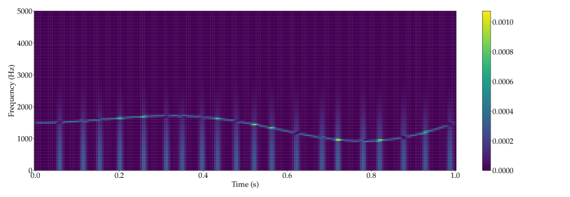
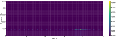
We generate a 1-second mixture, sampled at Hz (i.e., samples). The bumps signal is composed of about 20 randomly spaced bumps, while ensuring that ms. The bumps have a Hann window shape, where ms (i samples). The AM-FM signal has a single component, with a constant amplitude, and an instantaneous frequency defined by
where kHz is the central frequency. Figure 1 shows the resulting mixture spectrogram. The analysis window is a Hann window of length ms. This satisfies Inequality (6), ensuring non-interference between the bumps in the spectrogram of the bumps signal.
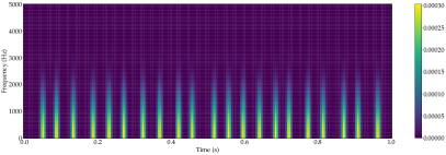
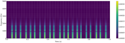
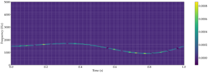
We run the proposed algorithm with . We observe that the algorithm converges in iterations. Figure 2 shows the estimated spectrograms of and in the left panels. We note that the two components are indeed separated in the time-frequency plane. The intrinsic characteristics of the spectrograms are well preserved, with smoothness regarding frequency for the first component, and sparsity for the second. However, challenges arise in regions of overlap, making component separation more challenging and leading to some distortions. The spectrograms estimated using NMF are shown in the right panels of Figure 2. While NMF accurately captures the vertical patterns of the first component, the estimated second component exhibits a spectrogram resembling a discontinuous horizontal line, diverging significantly from the expected pattern. The additional degree of freedom offered by our method allows for a more accurate decomposition of the spectrogram. Indeed, the norm of residuals after convergence is with our algorithm while it is with NMF.
IV-B Application to an audio signal
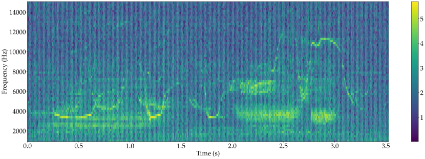
We analyze a -second recording of a vocalizing Atlantic spotted dolphin. It is sourced from the Watkins Marine Mammal Sound Database [25]. The sound the dolphin produces is made up of whistles and clicks. The bumps signal models the clicks, whereas the AM-FM component models the whistles. The spectrogram of the sound is shown in Figure 3. The contributions of the two components are visible in the time-frequency plane.
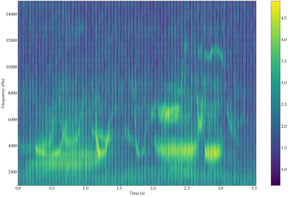
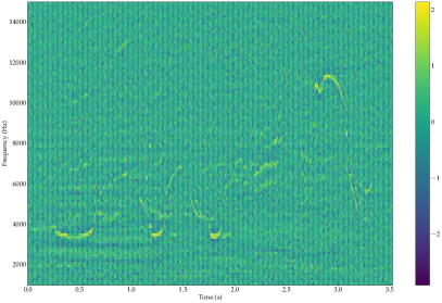
We set and . The algorithm converges in iterations. The estimated spectrograms, shown in Figure 4, illustrate the ability of our technique to isolate the two components in the time-frequency plane. On the one hand, the estimated spectrogram of the bumps component is a frequency-spread representation, especially visible during click periods (e.g., in the 2–3 s interval). On the other hand, the estimated spectrogram of the AM-FM signal captures the frequency-localized whistles (visible, e.g., around 4-6 kHz in the 0–2 s interval). This example shows the extent to which this tool can be used in bioacoustics to better visualize and interpret the two types of sound emitted simultaneously by a dolphin.
V Conclusion and Perspectives
We have presented a consistent spectrogram separation technique, adapted to a specific type of nonstationary mixtures composed of a bump component and an AM-FM component. To address this problem, we leveraged the properties of the time-frequency representations of such mixtures. We then constructed an inverse problem to estimate the spectrograms of the two components. Finally, we propose an alternating optimization algorithm that we test on a synthetic mixture. We show that our method outperforms the standard NMF decomposition. An application to a bioacoustic signal is also presented, demonstrating the real-world applicability of the technique.
This work represents a step towards the construction of a single-channel source separation method for reconstructing the two components themselves. We plan to use the estimated spectrograms as time-frequency masks to estimate the STFTs of each component. Our previous work is particularly well-suited to this type of problem [26]. An inverse transform will then be used to reconstruct the time signals.
Appendix: Proof of Theorem 1
Proof.
By incorporating the bumps signal expression (2) into the STFT definition (4), we obtain
The second row is obtained by changing the variable . Besides, since and are compactly supported functions, is nonzero only if the supports of and intersect. This condition is written
| (13) |
Hence, and are never simultaneously nonzero if there is no value of where (13) is satisfied for and simultaneously. We end up with the condition
which is always satisfied when (6) is true. Therefore, the spectrogram is given by
This yields
| (14) |
Besides, the analysis window had wider support than . That is why we take advantage of the mean value theorem to write:
| (15) |
Hence,
| (16) |
where . The same reasoning yields
| (17) |
where . Inserting results (16) and (17) into Equation (14) leads to the main result (7) of the theorem. Finally, we bound the error terms as follows:
∎
References
- [1] A. M. Reddy and B. Raj, “Soft mask methods for single-channel speaker separation,” IEEE Transactions on Audio, Speech and Language Processing, vol. 15, pp. 1766–1776, Aug. 2007.
- [2] Z. Rafii and B. Pardo, “A simple music/voice separation method based on the extraction of the repeating musical structure,” 2011 IEEE International Conference on Acoustics, Speech and Signal Processing (ICASSP), pp. 221–224, 2011.
- [3] J. R. Hershey, Z. Chen, J. Le Roux, and S. Watanabe, “Deep clustering: Discriminative embeddings for segmentation and separation,” in 2016 IEEE International Conference on Acoustics, Speech and Signal Processing (ICASSP), pp. 31–35, 2016.
- [4] J.-F. Aujol, G. Gilboa, T. Chan, and S. Osher, “Structure-texture image decomposition—modeling, algorithms, and parameter selection,” International journal of computer vision, vol. 67, pp. 111–136, 2006.
- [5] L. Benaroya, F. Bimbot, and R. Gribonval, “Audio source separation with a single sensor,” IEEE Transactions on Audio, Speech and Language Processing, vol. 14, pp. 191–199, Jan. 2006.
- [6] J. Hopgood and P. Rayner, “Single channel separation using linear time varying filters: separability of non-stationary stochastic signals,” in 1999 IEEE International Conference on Acoustics, Speech, and Signal Processing. Proceedings. ICASSP99 (Cat. No.99CH36258), IEEE, 1999.
- [7] T. Kristjansson, H. Attias, and J. Hershey, “Single microphone source separation using high resolution signal reconstruction,” in 2004 IEEE International Conference on Acoustics, Speech, and Signal Processing, ICASSP-04, IEEE, 2004.
- [8] B. H. Juang and L. R. Rabiner, “Hidden markov models for speech recognition,” Technometrics, vol. 33, pp. 251–272, Aug. 1991.
- [9] T. Virtanen, “Speech recognition using factorial hidden markov models for separation in the feature space,” in Interspeech 2006, interspeech_2006, ISCA, Sept. 2006.
- [10] L. A. Drake, J. C. Rutledge, J. Zhang, and A. Katsaggelos, “A computational auditory scene analysis-enhanced beamforming approach for sound source separation,” EURASIP Journal on Advances in Signal Processing, vol. 2009, Oct. 2009.
- [11] E. M. Grais, M. U. Sen, and H. Erdogan, “Deep neural networks for single channel source separation,” in 2014 IEEE International Conference on Acoustics, Speech and Signal Processing (ICASSP), IEEE, May 2014.
- [12] G.-J. Jang and T.-W. Lee, “A maximum likelihood approach to single-channel source separation,” The Journal of Machine Learning Research, vol. 4, p. 1365–1392, 10 2004.
- [13] M. Gales and S. Young, “The application of hidden markov models in speech recognition,” Foundations and Trends® in Signal Processing, vol. 1, no. 3, pp. 195–304, 2007.
- [14] S. T. Roweis, “One microphone source separation,” in Neural Information Processing Systems, 2000.
- [15] M. A. Casey and A. Westner, “Separation of mixed audio sources by independent subspace analysis,” in International Conference on Mathematics and Computing, 2000.
- [16] M. N. Schmidt and R. K. Olsson, “Single-channel speech separation using sparse non-negative matrix factorization,” in Interspeech 2006, interspeech_2006, ISCA, Sept. 2006.
- [17] E. M. Grais and H. Erdogan, “Single channel speech music separation using nonnegative matrix factorization and spectral masks,” in 2011 17th International Conference on Digital Signal Processing (DSP), IEEE, July 2011.
- [18] C. Févotte, E. Vincent, and A. Ozerov, Single-Channel Audio Source Separation with NMF: Divergences, Constraints and Algorithms, pp. 1–24. Springer International Publishing, 2018.
- [19] P. Comon and C. Jutten, Handbook of Blind Source Separation: Independent component analysis and applications. Academic press, 2010.
- [20] K. Yatabe, “Consistent ICA: Determined BSS meets spectrogram consistency,” IEEE Signal Processing Letters, vol. 27, pp. 870–874, 2020.
- [21] N. E. Huang, Z. Shen, S. R. Long, M. C. Wu, H. H. Shih, Q. Zheng, N.-C. Yen, C. C. Tung, and H. H. Liu, “The empirical mode decomposition and the Hilbert spectrum for nonlinear and non-stationary time series analysis,” Proceedings of the Royal Society of London. Series A: mathematical, physical and engineering sciences, vol. 454, no. 1971, pp. 903–995, 1998.
- [22] F. Auger, P. Flandrin, Y.-T. Lin, S. McLaughlin, S. Meignen, T. Oberlin, and H.-T. Wu, “Time-frequency reassignment and synchrosqueezing: An overview,” IEEE Signal Processing Magazine, vol. 30, no. 6, pp. 32–41, 2013.
- [23] M. Kowalski, A. Meynard, and H.-t. Wu, “Convex optimization approach to signals with fast varying instantaneous frequency,” Applied and computational harmonic analysis, vol. 44, no. 1, pp. 89–122, 2018.
- [24] A. Beck and M. Teboulle, “A fast iterative shrinkage-thresholding algorithm for linear inverse problems,” SIAM Journal on Imaging Sciences, vol. 2, pp. 183–202, Jan. 2009.
- [25] L. Sayigh, M. A. Daher, J. Allen, H. Gordon, K. Joyce, C. Stuhlmann, and P. Tyack, “The Watkins Marine Mammal Sound Database: an online, freely accessible resource,” Proceedings of Meetings on Acoustics, vol. 27, no. 1, p. 040013, 2016.
- [26] A. M. Krémé, V. Emiya, C. Chaux, and B. Torrésani, “Time-frequency fading algorithms based on Gabor multipliers,” IEEE Journal of Selected Topics in Signal Processing, vol. 15, no. 1, pp. 65–77, 2021.