Eluding Zeno effect via dephasing and detuning

Abstract

We analyze some variants of the Zeno effect in which the frequent observation of the population of an intermediate state does not prevent the transition of the system from the initial state to a certain final state. The Zeno effect is eluded by means of phase shifts or detunings that tailor the dynamics by suitably altering the interference governing quantum evolution.

I Introduction

The Zeno effect is the alteration of the free dynamics of a system when it is observed. It was initially introduced in the quantum domain as the inhibition of the evolution of a system that is forced by observation to remain in the initial state because of the measurement-induced quantum-state reduction MS77 ; IHBW90 ; PLG14 . Since then, the Zeno effect has been shown to be a dynamical effect decoupled from the reduction postulate AS94 ; PN94 ; VG95 ; LP96 ; SP97 , it has also been found in the classical domain YIK01 ; PLGS11 ; GPL15 , and it has been shown that it can not only inhibit evolution, but also accelerate it AL98 ; KK00 ; FGR01 ; AL02 ; AL03 , providing in general a suitable subtle way to influence on the dynamics FGMPS00 ; AL01 ; FP02 ; FP08 ; AL11 ; SHCLCCS14 ; LS95 .

Much of these results point to a fundamental principle of the evolution of quantum and wavelike systems in general. This is that evolution operates under principles of coherence and interference, as well illustrated by the Huygens-Fresnel principle within the wave theory of light. Inhibition of the observed dynamics can be understood as caused by observation-induced incoherence that prevents constructive interference typical of evolution, while acceleration of the dynamics occurs when decoherence inhibits destructive interference.

In this work we intend to advance in the knowledge of the physical mechanisms that operate behind the different versions of the Zeno effect. For this purpose we consider a system which can freely evolve from an initial state $A1$ to a final state $A2$ passing through an intermediate state $B$. A sufficiently precise observation of whether the system has reached $B$ naturally translates into inhibition of the evolution so that the system is frozen in the initial state $A1$ no longer being able to reach $A2$. And here is where we consider interesting to introduce variants, involving detunings or phase shifts, that impinge on the interferometric character of evolution. Such simple variations of the standard scheme allow the system to transit from state $A1$ to $A2$ although the measurements confirm that it never passed through state $B$. The result, which is paradoxical in defying the common intuition, is intelligible as a consequence of the concepts of coherence and interference, which are inherent to evolution in quantum and wavelike systems in general.

II Scheme and main goal

Our scheme is made of a chain of three harmonic oscillators, $A1$, $A2$ and $B$, coupled as illustrated in Fig. 1. For definiteness we will consider them to be three independent modes of the electromagnetic field. Modes $A1$ and $A2$ have the same frequency, being both coupled to $B$, while there is no direct coupling between $A1$ and $A2$, as schematized in Fig. 1. The Hamiltonian of the system, in interaction picture is

$$H=\kappa_{1}\left(a_{1}^{\dagger}b+a_{1}b^{\dagger}\right)+\kappa_{2}\left(a_{2}^{\dagger}b+a_{2}b^{\dagger}\right)-\Delta b^{\dagger}b,$$ (1)

where $a_{1},a_{2}$ and $b$ are the corresponding complex-amplitude operators, $\kappa_{1}$ and $\kappa_{2}$ are the coupling parameters, and $\Delta$ is the detuning of mode $B$ with respect to modes $A1$, $A2$.

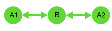
Figure 1: Chain of three coupled harmonic oscillators. Initially only $A1$ is excited. We study the propagation of the excitation form $A1$ to $A2$ depending on the observation of whether the excitation passes through $B$ or not.

To illustrate the main ideas we will consider a single-photon excitation, initially allocated in mode $A1$. In case of free evolution the photon will evolve to mode $B$ and once there it can evolve to mode $A2$. Then we consider the effect of observation of the population of the intermediate mode $B$. The Zeno logic would say that the frequent observation of whether the photon is in mode $B$ will prevent the transition form $A1$ to $B$ so there will be no chance for the photon to go into the $A2$ mode.

We will show that this is actually the case in the most simple and standard form of Zeno effect. But we can also show that very simple departures from the standard scenario, simply addding detunig and dephasing, allow the transition from $A1$ to $A2$ even under an arbitrarily precise monitoring of the intermediate mode $B$.

III Observed dynamics

Free evolution is given by the unitary operator exponential of the Hamiltonian as usual $U=\exp(-iHt)$. Initially, all the light will be concentrated in mode $A1$, while modes $A2$ and $B$ will be initially in their vacuum states $|0\rangle_{2}$, $|0\rangle_{b}$. Free evolution of duration $\delta t$ will be interrupted periodically at some given times $t_{j}=j\delta t$ to check whether mode $B$ is in the vacuum state or not. We will consider only those events in which the observation finds the mode $B$ in vacuum. This means that the reduced evolution in modes $A1$ and $A2$ is given by a sequence of nonunitary transformation

$$|\Psi_{j}\rangle=V_{j}|\Psi_{j-1}\rangle,\quad V_{j}={}_{b}\langle 0|e^{-iH\delta t}|0\rangle_{b}$$ (2)

where $|\Psi_{j}\rangle$ is the state in modes $A1$, $A2$ at times $t_{j}=j\delta t$, being the initial state $|\Psi_{0}\rangle=|\psi\rangle_{1}|0\rangle_{2}$, with $|\psi\rangle$ is in principle an arbitrary state. Later we will include the possibility that the observation introduces a random phase shift at each measurement step.

Let us consider a simple mode transformation simplifying calculus. This is a transformation from modes $A1$, $A2$ to some newly defined modes $A$ and $C$ with complex amplitude operators $a$ and $c$

$$a=\cos{\theta}a_{1}+\sin{\theta}a_{2},\quad c=-\sin{\theta}a_{1}+\cos{\theta}a_{2},$$ (3)

such that Hamiltonian (1) reads

$$H=\kappa\left(a^{\dagger}b+ab^{\dagger}\right)-\Delta b^{\dagger}b,$$ (4)

where

$$\cos\theta=\frac{\kappa_{1}}{\kappa},\;\sin\theta=\frac{\kappa_{2}}{\kappa},\quad\kappa=\sqrt{\kappa_{1}^{2}+\kappa_{2}^{2}},$$ (5)

and the proper commutations rules are satisfied

$$\left[a,a^{\dagger}\right]=\left[c,c^{\dagger}\right]=1,\quad\left[a,c\right]=\left[a,c^{\dagger}\right]=0.$$ (6)

Let us construct the operator $V_{j}$. We can begin by noting that, after Ref. LS95

$$e^{-iH\delta t}ae^{iH\delta t}=e^{-i\Delta\delta t/2}\left(\mu^{\ast}a+\nu^{\ast}b\right),$$ (7)

where

$$\mu=\cos(\gamma\delta t)-i\frac{\Delta}{2\gamma}\sin(\gamma\delta t),\quad\nu=-i\frac{\kappa}{\gamma}\sin\gamma,$$ (8)

being

$$\gamma=\sqrt{\kappa^{2}+\Delta^{2}/4}.$$ (9)

Then let us consider the most general pure state $|\Psi\rangle$ in modes $A1$, $A2$ expressed in the photon-number basis as

$$|\Psi\rangle=\sum_{n_{1},n_{2}}c_{n_{1},n_{2}}a_{1}^{\dagger n_{1}}a_{2}^{\dagger n_{2}}|0\rangle_{1}|0\rangle_{2}.$$ (10)

This is, after inverting Eqs. (3)

$$|\Psi\rangle=\sum_{n_{1},n_{2}}c_{n_{1},n_{2}}\left(\cos{\theta}a^{\dagger}-\sin{\theta}c^{\dagger}\right)^{n_{1}}$$

$$\times\left(\sin{\theta}a^{\dagger}+\cos{\theta}c^{\dagger}\right)^{n_{2}}|0\rangle_{1}|0\rangle_{2},$$ (11)

so that after Eq. (7)

$$e^{-iH\delta t}|\Psi\rangle|0\rangle_{b}=\sum_{n_{1},n_{2}}c_{n_{1},n_{2}}$$

$$\times\left[e^{i\Delta\delta t/2}\cos{\theta}\left(\mu a^{\dagger}+\nu b^{\dagger}\right)-\sin{\theta}c^{\dagger}\right]^{n_{1}}$$

$$\times\left[e^{i\Delta\delta t/2}\sin{\theta}\left(\mu a^{\dagger}+\nu b^{\dagger}\right)+\cos{\theta}c^{\dagger}\right]^{n_{2}}|0\rangle_{1}|0\rangle_{2},$$

and then projecting on the vacuum state in mode $B$

$${}_{b}\langle 0|e^{-iH\delta t}|0\rangle_{b}|\Psi\rangle=\sum_{n_{1},n_{2}}c_{n_{1},n_{2}}$$

$$\times\left(e^{i\Delta\delta t/2}\cos{\theta}\mu a^{\dagger}-\sin{\theta}c^{\dagger}\right)^{n_{1}}$$

$$\times\left(e^{i\Delta\delta t/2}\sin{\theta}\mu a^{\dagger}+\cos{\theta}c^{\dagger}\right)^{n_{2}}|0\rangle_{1}|0\rangle_{2}.$$ (13)

This is equal to say that

$${}_{b}\langle 0|e^{-iH\delta t}|0\rangle_{b}|\Psi\rangle=V_{j}|\Psi\rangle,$$ (14)

where

$$V_{j}=\chi_{j}^{a^{\dagger}a},\quad\chi_{j}=e^{i\phi_{j}}e^{i\Delta\delta t/2}\mu,$$ (15)

and we have already included the possibility that the measurement induces a phase shift $\phi_{j}$ in mode $A$ as a kind of measurement back action. The equivalence in Eqs. (14) and (15) follows after using that for every function $f(a^{\dagger}a)$ we have $f(a^{\dagger}a)a^{\dagger}=a^{\dagger}f(a^{\dagger}a+1)$, and then

$$V_{j}a^{\dagger}V_{j}^{-1}=\chi_{j}a^{\dagger},$$ (16)

along with $V_{j}|0\rangle_{1}|0\rangle_{2}=|0\rangle_{1}|0\rangle_{2}$ .

Then the complete evolution after $n$ successful measurements checking that mode $B$ is in the vacuum state is

$$|\Psi_{n}\rangle=V|\Psi_{0}\rangle,$$ (17)

with

$$V=\Pi_{j=1}^{n}V_{j}=\chi^{a^{\dagger}a},$$ (18)

and

$$\chi=\Pi_{j=1}^{n}\chi_{j}=e^{i\phi}e^{i\Delta n\delta t/2}\mu^{n},$$ (19)

being $\phi$ the accumulated dephasing

$$\phi=\sum_{j=1}^{n}\phi_{j}.$$ (20)

Then

$$Va^{\dagger}V^{-1}=\chi a^{\dagger},$$ (21)

along with $V|0\rangle_{1}|0\rangle_{2}=|0\rangle_{1}|0\rangle_{2}$ .

Throughout the above analysis the states $|\Psi_{j}\rangle$ are not normalized being the norm the success probability, this is the probability that all measurements find the mode $B$ in the vacuum state

$$P(n,\delta t)=\langle\Psi_{n}|\Psi_{n}\rangle=\langle\Psi_{0}|V^{\dagger}V|\Psi_{0}\rangle.$$ (22)

On what follows we will consider three meaningful cases, all them always in the limit of arbitrarily accurate monitoring of mode $B$, this is with $\delta t=t/n$ for a fixed time interval $t$. These three cases are:

• Standard Zeno effect, with no dephasing $\phi=0$ and no detuning $\Delta=0$.

• Dephasing $\phi_{j}\neq 0$ with no detuning $\Delta=0$.

• Detuning $\Delta\neq 0$ with no dephasing $\phi=0$.

IV One-photon case

Let us consider the simple but fully meaningful case of a single photon initially in mode $A1$ at $t=0$, this is

$$|\Psi_{0}\rangle=|1\rangle_{1}|0\rangle_{2},$$ (23)

which in modes in modes $A$, $C$ becomes

$$|\Psi_{0}\rangle=\cos\theta|1\rangle_{a}|0\rangle_{c}-\sin\theta|0\rangle_{a}|1\rangle_{c}.$$ (24)

The observed dynamics readily follows after applying Eq. (17) leading to

$$|\Psi_{n}\rangle=\chi\cos\theta|1\rangle_{a}|0\rangle_{c}-\sin\theta|0\rangle_{a}|1\rangle_{c},$$ (25)

that in modes $A1$, $A2$ reads

$$|\Psi_{n}\rangle=\zeta_{1}|1\rangle_{1}|0\rangle_{2}+\zeta_{2}|0\rangle_{1}|1\rangle_{2},$$ (26)

with

$$\zeta_{1}=\chi\cos^{2}\theta+\sin^{2}\theta,$$

(27)

$$\zeta_{2}=\left(\chi-1\right)\cos\theta\sin\theta,$$

where $\chi$ is in Eq. (19). The probability that all the $n$ measurements find mode B in the vacuum state is

$$P(n,\delta t)=|\zeta_{1}|^{2}+|\zeta_{2}|^{2}.$$ (28)

The main goal is whether the photon can be found in mode $A2$ without having been found in mode $B$. The corresponding conditional probability is

$$p(n,\delta t)=\frac{|\zeta_{2}|^{2}}{|\zeta_{1}|^{2}+|\zeta_{2}|^{2}}.$$ (29)

We are going to examine these probabilities in the scenarios considered above.

IV.1 No dephasing $\phi=0$, no detuning $\Delta=0$

In this case

$$\zeta_{1}=\cos^{n}(\kappa\delta t)\cos^{2}\theta+\sin^{2}\theta,$$

(30)

$$\zeta_{2}=\left[\cos^{n}(\kappa\delta t)-1\right]\cos\theta\sin\theta.$$

In the limit of arbitrarily accurate monitoring of mode $B$, this is with $\delta t=t/n$ for a fixed time interval $t$ and $n\rightarrow\infty$ we have:

$$\lim_{n\rightarrow\infty}\cos^{n}(\kappa t/n)=1$$ (31)

so that

$$\zeta_{1}\rightarrow 1,\qquad\zeta_{2}\rightarrow 0,$$ (32)

this is

$$P(n,\delta t)\rightarrow 1,\qquad p(n,\delta t)\rightarrow 0,$$ (33)

and the evolution tends to be completely frozen the photon remaining always in mode $A1$.

IV.2 Dephasing $\phi\neq 0$, no detuning $\Delta=0$

In this case

$$\zeta_{1}=e^{i\phi}\cos^{n}(\kappa\delta t)\cos^{2}\theta+\sin^{2}\theta,$$

(34)

$$\zeta_{2}=\left[e^{i\phi}\cos^{n}(\kappa\delta t)-1\right]\cos\theta\sin\theta.$$

In the same limit of arbitrarily accurate monitoring of mode $B$, this is with $\delta t=t/n$ for a fixed time interval $t$ and $n\rightarrow\infty$ we have:

$$\zeta_{1}\rightarrow e^{i\phi}\cos^{2}\theta+\sin^{2}\theta,$$

(35)

$$\zeta_{2}\rightarrow\left(e^{i\phi}-1\right)\cos\theta\sin\theta,$$

with the following probabilities of success in finding the mode $B$ always in vacuum

$$P(n,\delta t)\rightarrow 1,$$ (36)

and conditional probability that the photon is found in mode $A2$

$$p(n,\delta t)\rightarrow 2\cos^{2}\theta\sin^{2}\theta\left(1-\cos\phi\right).$$ (37)

In this case we get that the photon is never in mode $B$ while it can be successfully transferred from mode $A1$ to mode $A2$.

This is counter intuitive as we have reasoned above. Actually the transfer can be complete $p(n,\delta t)\rightarrow 1$ in the case of $\phi=(2m+1)\pi$ for integer $m$ and $\kappa_{1}=\kappa_{2}$, this is $\theta=\pi/4$. This is assuming $\phi$ to be deterministic. If otherwise we consider it as fully random, by averaging over fully random $\phi_{j}$ we get

$$p(n,\delta t)\rightarrow 2\cos^{2}\theta\sin^{2}\theta=2\frac{\kappa_{1}^{2}\kappa_{2}^{2}}{\left(\kappa_{1}^{2}+\kappa_{2}^{2}\right)^{2}},$$ (38)

which reaches its maximum value $p(n,\delta t)\rightarrow 1/2$ for $\kappa_{1}=\kappa_{2}$.

IV.3 Detuning $\Delta\neq 0$, no dephasing $\phi=0$

In order to take full advantage of the detuning let us consider the case of rather strong detuning $\Delta\gg\kappa$ so that

$$e^{i\Delta\delta t/2}\mu\simeq e^{-i(\kappa^{2}/\Delta)\delta t},$$ (39)

and then

$$\zeta_{1}\simeq e^{-i(\kappa^{2}/\Delta)n\delta t}\cos^{2}\theta+\sin^{2}\theta$$

(40)

$$\zeta_{2}\simeq\left[e^{-i(\kappa^{2}/\Delta)n\delta t}-1\right]\cos\theta\sin\theta.$$

Again in the limit of arbitrarily accurate monitoring of mode $B$, this is with $\delta t=t/n$ for a fixed time interval $t$, we have that $\zeta_{1}$ and $\zeta_{2}$ no longer depend on $n$ and we get the following probabilities of success in finding the mode $B$ always in vacuum

$$P(n,\delta t)\simeq 1,$$ (41)

and the following conditional probability that the photon is found in mode $A2$

$$p(n,\delta t)\rightarrow 2\cos^{2}\theta\sin^{2}\theta\left[1-\cos\left(\kappa^{2}t/\Delta\right)\right].$$ (42)

Once again, in this case we get that the photon is never in mode $B$ while it can transferred from mode $A1$ to mode $A2$.

Roughly speaking, in the strong detuning case, the free evolution will never populate the mode $B$, so the measurement has actually no effect. If our system would be just modes $A1$ and $B$ the photon would remain always in the initial mode $A1$. However the coupling of mode $B$ with mode $A2$ allows the migration of the photon from $A1$ to $A2$. This is still counter intuitive and may be pictured as mediated through some virtual intermediate mode different from $B$.

V Multi-photon states

We can easily show that the results obtained for a single photon are reproduced by other initial field states in mode $A1$. As an illustrative example let us comment briefly on the cases of number and Glauber coherent states.

V.1 Number states

Let us consider that the initial state in mode $A1$ is a photon-number state:

$$|\Psi_{0}\rangle=|N\rangle_{1}|0\rangle_{2}=\frac{1}{\sqrt{N!}}a^{\dagger N}_{1}|0\rangle_{1}|0\rangle_{2},$$ (43)

that in modes $A$ and $C$ reads

$$|\Psi_{0}\rangle=\frac{1}{\sqrt{N!}}\left(\cos{\theta}a^{\dagger}-\sin{\theta}c^{\dagger}\right)^{N}|0\rangle_{a}|0\rangle_{c}.$$ (44)

After Eqs. (17) and (21) we get

$$|\Psi_{n}\rangle=\frac{1}{\sqrt{N!}}\left(\zeta_{1}a^{\dagger}_{1}+\zeta_{2}a^{\dagger}_{2}\right)^{N}|0\rangle_{1}|0\rangle_{2}.$$ (45)

leading to

$$|\Psi_{n}\rangle=\sum_{j=0}^{N}\left(\begin{matrix}N\\ j\end{matrix}\right)^{1/2}\zeta_{1}^{N-j}\zeta_{2}^{j}|N-j\rangle_{1}|j\rangle_{2},$$ (46)

where $\zeta_{1}$, $\zeta_{2}$ are the same in Eq. (IV). The probability that the $n$ measurements find the mode $B$ in vacuum is

$$P(n,\delta t)=\langle\Psi_{n}|\Psi_{n}\rangle=\left(|\zeta_{1}|^{2}+|\zeta_{2}|^{2}\right)^{N}.$$ (47)

In this case we can measure the amount of light transferred to the $A2$ by the mean number of photons:

$$\frac{\langle\Psi_{n}|a^{\dagger}_{2}a_{2}|\Psi_{n}\rangle}{\langle\Psi_{n}|\Psi_{n}\rangle}=N\frac{|\zeta_{2}|^{2}}{|\zeta_{1}|^{2}+|\zeta_{2}|^{2}}.$$ (48)

Therefore, we find these are a simple scaled versions of the one-photon results in Eqs. (28) and (29).

V.2 Coherent states

Let us consider that the initial state in mode $A1$ is a Glauber coherent state:

$$|\Psi_{0}\rangle=|\alpha\rangle_{1}|0\rangle_{2},$$ (49)

where $|\alpha\rangle_{1}$ is a Glauber coherent state, eigenvector of the complex-amplitude operator, which can be expressed as

$$|\Psi_{0}\rangle=e^{-|\alpha|^{2}/2}e^{\alpha a_{1}^{\dagger}}|0\rangle_{1}|0\rangle_{2}.$$ (50)

Following the same steps already followed above we find

$$|\Psi_{n}\rangle=e^{-|\alpha|^{2}[1-|\zeta_{1}|^{2}-|\zeta_{2}|^{2}]/2}|\alpha\zeta_{1}\rangle_{1}|\alpha\zeta_{2}\rangle_{2},$$ (51)

where $|\alpha\zeta_{1}\rangle_{1}|\alpha\zeta_{2}\rangle_{2}$ are normalized Glauber coherent states with $\zeta_{1}$, $\zeta_{2}$ in Eq. (IV). So, all the results found in the one-photon can can be equally repeated here in all the observation scenarios considered, again with the same conclusions.

It can be seen that a series of powers on $\alpha$ of the coherent case actually reproduces the number case, including the one-photon example. In this regard, in the limit of arbitrarily precise observation of mode $B$ we get that $V$ approaches the unitary operator

$$V\rightarrow e^{i\left(\phi-\kappa^{2}t/\Delta\right)a^{\dagger}a},$$ (52)

which is a phase shift in mode $A$ and a lossless beam splitter in modes $A1$ and $A2$. So the cases considered in this work, number and coherent, behave alike because of the complex-amplitude operator transformation induced by this effective beam splitter that underlies all the cases examined.

VI Conclusions

We have analyzed some variants of the Zeno effect in which exhaustive observation of the population of an intermediate state does not prevent the transition of the system from the initial state to a certain final state. The result can be understood as paradoxical since, according to the most standard version of the Zeno effect, the precise observation of the occupation of the intermediate state freezes the system in the initial state so never evolves to the final state.

In our case the evolution to the final state is allowed in spite of the frequent observation. This is because dephasing and detuning alter the interference that is always behind any quantum or wavelike evolution. We can recall that the different versions of Zeno effect are actually interferometric in nature, because measurement-induced back action impedes constructive or destructive interference, depending on the context.

A very suggestive feature of the cases we have discussed here is that they invoke physical processes that in other contexts mark the transition from quantum to classical physics. For example, decoherence caused by random phases is a known mechanism of emergence of the classical world from the quantum one, something that has already been studied precisely in this same context of the Zeno effect WHZ03 ; LAL20 . On the other hand, the lack of resonance guarantees, for example, that in the interaction of light with matter the classical Lorentz model of the atom is perfectly valid.

References

- (1) Misra and E. C. G. Sudarshan, The Zeno’s paradox in quantum theory, J. Math. Phys. 18, 756–763 (1977).
- (2) W. M. Itano, D. J. Heinzen, J. J. Bollinger, and D. J. Wineland, Quantum Zeno effect, Phys. Rev. A 41, 2295–2300 (1990).
- (3) M. A. Porras, A. Luis, and I. Gonzalo, Quantum Zeno effect for a free-moving particle, Phys. Rev. A 90, 062131 (2014).
- (4) T. P. Altenmüller and A. Schenzle, Quantum Zeno effect in a double-well potential: A model of a physical measurement, Phys. Rev. A 49, 2016–2027 (1994).
- (5) S. Pascazio and M. Namiki, Dynamical quantum Zeno effect, Phys. Rev. A 50, 4582–4592 (1994).
- (6) A. Venugopalan and R. Ghosh, Decoherence and the quantum Zeno effect, Phys. Lett. A 204, 11–15 (1995).
- (7) A. Luis and J. Peřina, Zeno effect in parametric down-conversion, Phys. Rev. Lett. 76, 4340–4343 (1996).
- (8) S. Pascazio, Dynamical origin of the quantum Zeno effect, Found Phys 27, 1655–1670 (1997).
- (9) K. Yamane, M. Ito, and M. Kitano, Quantum Zeno effect in optical fibers, Opt. Commun. 192, 299–307 (2001).
- (10) M.A. Porras, A. Luis, I. Gonzalo, and A.S. Sanz, Zeno dynamics in wave-packet diffraction spreading, Phys. Rev. A 84, 052109 (2011).
- (11) I. Gonzalo, M. A. Porras, and A. Luis, Zeno inhibition of polarization rotation in an optically active medium, Eur. J. Phys. 36, 045001 (2015).
- (12) A. Luis, Anti–Zeno effect in parametric down-conversion, Phys. Rev. A 57, 781–787 (1998).
- (13) A. G. Kofman and G. Kurizki, Acceleration of quantum decay processes by frequent observations, Nature 405, 546–550 (2000).
- (14) M. C. Fischer, B. Gutiérrez-Medina, and M. G. Raizen, Observation of the quantum Zeno and anti-Zeno effects in an unstable system, Phys. Rev. Lett. 87, 040402 (2001).
- (15) A. Luis, Zeno and anti-Zeno effects in multimode parametric down-conversion, Phys. Rev. A 66, 012101 (2002).
- (16) Zeno and anti-Zeno effects in two-level systems, Phys. Rev. A 67, 062113 (2003).
- (17) F. Facchi, V. Gorini, G. Marmo, S. Pascazio, and E.C.G. Sudarshan, Quantum Zeno dynamics, Phys. Lett. A 275, 12–19 (2000).
- (18) A. Luis, Construction of a matter-light interferometer via the Zeno effect, J. Opt. B: Quantum and Semiclass. Opt. 3, 238–241 (2001).
- (19) P. Facchi and S. Pascazio, Quantum Zeno Subspaces, Phys. Rev. Lett. 89, 080401 (2002).
- (20) P. Facchi and S. Pascazio, Quantum Zeno dynamics: Mathematical and physical aspects,J. Phys. A: Math. Theor. 41, 493001 (2008).
- (21) A. Luis, Quantum-state preparation and control via the Zeno effect, Phys. Re. A 63, 052112 (2011).
- (22) F. Schäfer, I. Herrera, S. Cherukattil, C. Lovecchio, F. S. Cataliotti, F. Caruso, and A. Smerzi, Experimental realization of quantum Zeno dynamics, Nat. Commun. 5, 3194 (2014).
- (23) A. Luis and L. L. Sánchez-Soto Quantum Semiclass. Opt. 7 153–160 (1995).
- (24) W. H. Zurek, Decoherence and the transition from quantum to classical revisited, arXiv:quant-ph/0306072.
- (25) J. López, L. Ares, and A. Luis, Observed quantum dynamics: Classical dynamics and lack of Zeno effect, J. Phys. A: Math. Theor. 53, 375306 (2020).