Thermodynamics of a Non-canonical $f(\bar{R},\bar{T})$ gravity

Abstract

This work comprises a study of the thermodynamic behavior of modified $f(\bar{R},\bar{T})$ gravity, which had been developed based on a non-canonical theory known as K-essence theory. In this development, we use the Dirac-Born-Infeld (DBI) type of non-standard Lagrangian. We develop a modified first law and generalized second law of thermodynamics (GSLT) within the modified $f(\bar{R},\bar{T})$ gravity, where we consider the background metric to be the usual Friedmann-Lema$\hat{\text{i}}$tre-Robertson-Walker (FLRW) type. A graphical analysis of surface gravity has been performed for the modified FLRW metric via the $f(\bar{R},\bar{T})$ theory, which is different from the usual FLRW gravity through the usual $f(R,T)$ gravity. In the study of the thermodynamic behavior of the cosmos, we use two distinct kinds of scale factors: exponential and power law. Through the investigation of the modified GSLT, we have seen that during the initial phase of the universe, the entropy’s rate of change may be either negative or positive, contingent upon the value of the curvature constant. The negativity of the entropy change indicates that the modified GSLT is not feasible in that particular area for a particular curvature constant. These traits suggest that during the inflationary period, entropy might have been either negative or positive. It has also been seen that entropy saturates every curvature value at different time ranges, which indicates the heat death of the universe.

I Introduction

Some cosmological queries, such as the horizon, the monopole, and the flatness problem, remained unanswered by the standard Einstein’s gravitational theory. Furthermore, the fine-tuning problem  [1] requires scientists to modify the theory due to the significant disparity in energy density, which is of the order of $10^{120}$. In addition, the ‘Cosmic Coincidence Problem’  [2, 1] has nevertheless to be resolved within the framework of the standard $\Lambda$-Cold Dark Matter (henceforth $\Lambda$CDM) theory. The recent observational data  [3, 4, 5] implies the universe is driven by an exotic component called dark energy by almost $70\%$. In order to address the foregoing issues, a new modified theory was proposed under the name of $f(R)$ theory [6]. The Einstein-Hilbert (EH) action was considered to be contingent on the function of the Ricci scalar ($f(R)$) rather than merely $R$. Harko et al. [7] expanded upon this theory by integrating the trace of the energy momentum tensor $T$ into the function, resulting in the $f(R,T)$ theory. Over the period of the last several years, a number of fascinating works have been conducted in relation to this theory [8, 9, 10, 11, 12].

Meanwhile, in order to address the cosmological unsolved problems mentioned earlier, scientists have put forth various models, including non-canonical ones like K-essence. The K-essence theory, which is shown in [13, 14, 15, 16, 17, 18, 19, 20, 21, 22, 23, 24], is not the same as the usual relativistic scalar field theory. As demonstrated in [25, 26, 27] the non-canonical Lagrangian is the general one which can produce canonical Lagrangian under specific circumstances. The authors of [22, 23, 24] used the Dirac-Born-Infeld (DBI) type [28, 29, 30] non-standard Lagrangian to come up with the simplest form of the K-essence emergent metric $\bar{G}_{\mu\nu}$, which is not conformally equivalent to the usual gravitational metric $g_{\mu\nu}$. The non-canonical Lagrangian can have the form of $\mathcal{L}(X,\phi)=-V(\phi)F(X)$ [20, 14, 15] or $\mathcal{L}(X,\phi)=F(X)-V(\phi)$  [31, 32] or $\mathcal{L}(X,\phi)\equiv\mathcal{L}(X)=F(X)$ [16, 21] where $F(X)\equiv\mathcal{L}(X)(\neq X)$ is the non-canonical kinetic part with $X=\frac{1}{2}g_{\mu\nu}\nabla^{\mu}\phi\nabla^{\nu}\phi$, $V(\phi)$ is the canonical potential part. The underlying motivation of using non-canonical theory has been well-described in [33]. We discuss two main advantages of K-essence theory here [33]. Firstly, the radiation background is the only factor influencing the K-essence field’s behavior in the K-essence model until the dark energy-dominated era started. It eliminates the requirement for fine-tuning that the canonical model had. Secondly, it has the potential to produce a dark energy component in which the speed of sound ($c_{S}$) is always slower than the speed of light. Large angular scale cosmic microwave background (CMB) disturbances may be reduced by this characteristic. It has also been said that the K-essence theory can be used in a model of dark energy [22, 23, 34, 24] as well as from a gravitational point of view [37, 35, 36, 38] without taking into account the dark parts of the universe. Panda et al. [33] investigated the cosmic behaviors of the cosmos using a non-canonical Lagrangian within the framework of emergent $f(\bar{R},\bar{T})$ gravity. The researchers used the Lagrangian of the DBI type, denoted as $\mathcal{L}(X)=1-\sqrt{1-2X}$, to derive the Friedmann equations. They then computed the effective energy density ($\bar{\rho}$), pressure ($\bar{p}$) and the Equation of State (EoS) parameter ($\bar{\omega}$).

On the other hand, black hole thermodynamics reveals a captivating link between our empirical observations of black holes and the fundamental principles of thermodynamics. Black holes exhibit similarities to regular thermodynamic systems, despite being composed of empty spacetime. These properties involve entropy and temperature. The entropy of a black hole is tightly linked to the area of its event horizon, while the temperature is intimately connected to the intriguing phenomenon known as Hawking radiation. In simple terms, based on the principles of quantum physics and general relativity, a black hole can be thought of as a black body that gives off thermal radiation. The temperature of this radiation is directly linked to the surface gravity at the black hole’s horizon, while the entropy is tied to the area of the horizon. The Hawking temperature and horizon entropy, along with the black hole mass, follow the principles of the first law of thermodynamics  [39, 40, 41]. The entropy and temperature formulas for black holes show a certain degree of universality, which means that Einstein’s equations alone determine the size of the black hole’s horizon and the gravity of its surface. The finding of Bekenstein on black hole entropy provided evidence for a significant physical relationship between thermodynamics and gravity [41]. Based on Einstein gravity, the gravitational entropy $S$ relates to the black hole horizon area $A$ as $S=A/(4G)$, where $G$ is the gravitational constant and Hawking temperature $(T)$ is related to the surface gravity ($k_{sg}$) as $T=k_{sg}/2\pi$, which corresponds to the first law of thermodynamics [41, 39, 40]. The Clausius relation $TdS=dQ$ on all local acceleration horizons in the Rindler space–time combined with the relation $S\propto A$ allows for the derivation of Einstein equations, as demonstrated by Jacobson  [42]. Here, $dQ$ and $T$ stand for the energy flux across the horizon and the Unruh temperature [43] perceived by an accelerating observer just inside the horizon, respectively. This approach was used in several cosmological scenarios, such as the quasi-de Sitter inflationary universe [44, 45] and the dark energy-dominated realm [46]. It is to note that Cai and Kim [47] used the first law of thermodynamics to find the entropy of the apparent horizon in the Friedmann-Lemaı’tre-Robertson-Walker (FLRW) universe, taking into account any spatial curvature. On the other hand, later on Akbar and Cai [48] showed that the Friedmann equations in GR may be stated as follows at the apparent horizon: $dE=TdS+WdV$, where $W=\frac{1}{2}(\rho-p)$, $V$, $\rho$ and $p$ are respectively the work density, volume, energy density and pressure while $E=\rho V$ is the total energy within the apparent horizon.

Several modified theories of gravity have shown that thermodynamics and gravity are connected. These include scalar-tensor gravity [47, 49], Lovelock gravity [50, 51], Braneworld gravity [52], nonlinear gravity [53], and Gauss-Bonnet gravity [48]. To find an equilibrium thermodynamics of the apparent horizon in the expanding cosmological background, the authors of [49] used a large group of modified gravity theories with the Lagrangian density $f(R,\phi,X)$. In these theories, $R$ is the Ricci scalar and $X$ is the kinetic part of a scalar field $\phi$. Note that non-equilibrium representation of thermodynamics is necessary in $f(R)$ gravity and scalar-tensor theory in order to modify the Clausius relation to $TdS=\delta Q+d\bar{S}$. The additional entropy production term in this case is $d\bar{S}$ [48, 53, 54]. In the study [54], the authors establish the principles of thermodynamics in $f(R,T)$ gravity and demonstrate that the existence of a connection between matter and geometry, represented by the expression $f_{T}=\partial f(R,T)/\partial T$, prevents the attainment of an equilibrium state. In $f(R,T)$ gravity, the presence of the total energy exchange term ($q_{tot}$) indicates that there is an ongoing energy exchange that occurs with the horizon. There is always a non-zero entropy-producing term in this theory. According to the authors, the non-equilibrium description may be recognized as a consequence of energy flow happening both inside and beyond the apparent horizon. The absence of an equilibrium state is caused by the non-zero value of the $f_{T}$ term. If the Lagrangian is only dependent on the geometry, then the term $f_{T}$ becomes zero, resulting in the attainment of an equilibrium state. This phenomenon occurs in the context of $f(R)$ gravity. Additionally, they demonstrated that both the phantom and non-phantom phases of $f(R,T)$ gravity adhere to the Generalised Second Law of Thermodynamics (GSLT). This result is consistent with the hypothesis put out by Nojiri et al.  [55] that entropy might have a positive value even in the phantom period.

The objective of this research is to analyze the thermodynamic properties of the universe within the framework of K-essence $f(\bar{R},\bar{T})$ gravity. The underlying metric used for our investigation is the homogeneous and isotropic FLRW spacetime. This work involves six sections. The second section has been dedicated to a review of the non-standard theory of K-essence. Section III comprises a review of $f(\bar{R},\bar{T})$ gravity from the point of view of K-essence. In Section IV, we have studied the thermodynamics of $f(\bar{R},\bar{T})$ gravity. In particular, subsection IV-A is the formulation of the first law of thermodynamics and a comparative study of surface gravity between the usual FRW and modified FRW cases. Subsection IV-B derives the generalized second law of thermodynamics of the $f(\bar{R},\bar{T})$ gravity. In Section V, we focus on the study of first-order and second-order variations of entropy with time. Section VI is the conclusion.

II The K-essence

This section provides a concise overview of K-essence theory. The K-essence geometry involves the interaction of a scalar field with gravity, which may be described by the following action when the scalar field is minimally coupled to gravity [19, 20, 18, 22, 23, 24]:

$$S_{k}[\phi,g_{\mu\nu}]=\int d^{4}x{\sqrt{-}g}\mathcal{L}(X,\phi),$$ (1)

where $X=\frac{1}{2}g^{\mu\nu}\nabla_{\mu}\phi\nabla_{\nu}\phi$ is the canonical kinetic term and $\mathcal{L}(X,\phi)$ is the non-canonical Lagrangian. From the definition of the energy-momentum tensor:

$$T_{\mu\nu}\equiv\frac{-2}{\sqrt{-g}}\frac{\delta S_{k}}{\delta g^{\mu\nu}}=-2\frac{\partial\mathcal{L}}{\partial g^{\mu\nu}}+g_{\mu\nu}\mathcal{L}=-\mathcal{L}_{X}\nabla_{\mu}\phi\nabla_{\nu}\phi+g_{\mu\nu}\mathcal{L},$$ (2)

where $\mathcal{L}_{\mathrm{X}}=\frac{d\mathcal{L}}{dX},\leavevmode\nobreak\ \mathcal{L}_{\mathrm{X}X}=\frac{d^{2}\mathcal{L}}{dX^{2}},\leavevmode\nobreak\ \mathcal{L}_{\mathrm{\phi}}=\frac{d\mathcal{L}}{d\phi}$ and $\nabla_{\mu}$ is the covariant derivative defined with respect to the gravitational metric $g_{\mu\nu}$.

The corresponding scalar field equation of motion (EOM) is

$$-\frac{1}{\sqrt{-g}}\frac{\delta S_{k}}{\delta\phi}=\tilde{G}^{\mu\nu}\nabla_{\mu}\nabla_{\nu}\phi+2X\mathcal{L}_{X\phi}-\mathcal{L}_{\phi}=0,$$ (3)

where the effective metric is:

$$\tilde{G}^{\mu\nu}\equiv\frac{c_{s}}{\mathcal{L}_{X}^{2}}[\mathcal{L}_{X}g^{\mu\nu}+\mathcal{L}_{XX}\nabla^{\mu}\phi\nabla^{\nu}\phi]$$ (4)

with $1+\frac{2X\mathcal{L}_{XX}}{\mathcal{L}_{X}}>0$ and $c_{s}^{2}(X,\phi)\equiv{(1+2X\frac{\mathcal{L}_{XX}}{\mathcal{L}_{X}})^{-1}}$.

After a conformal transformation [22, 23, 24] $\bar{G}_{\mu\nu}\equiv\frac{c_{s}}{\mathcal{L}_{X}}G_{\mu\nu}$, we can write the inverse of the effective metric (4) as

$$\bar{G}_{\mu\nu}=g_{\mu\nu}-\frac{\mathcal{L}_{XX}}{\mathcal{L}_{X}+2X\mathcal{L}_{XX}}\nabla_{\mu}\phi\nabla_{\nu}\phi.$$ (5)

Equations (3)–(5) are physically relevant if $\mathcal{L}_{X}\neq 0$ is positive definite. In K-essence, Eq. (6) states that our emergent metric, $\bar{G}_{\mu\nu}$, is conformally different from $g_{\mu\nu}$ for non-trivial spacetime configurations of $\phi$. Unlike canonical scalar fields, $\phi$ has different local causal structural features. They also vary from those specified with $g_{\mu\nu}$.

By addressing the Lagrangian’s implicit dependency on $\phi$, the equation of motion (EOM) expressed in Eq. (3) becomes,

$$\frac{1}{\sqrt{-g}}\frac{\delta S_{k}}{\delta\phi}=\bar{G}^{\mu\nu}\nabla_{\mu}\nabla_{\nu}\phi=0.$$ (6)

Taking into account the non-canonical Lagrangian of the DBI type $\mathcal{L}(X,\phi)\equiv\mathcal{L}(X)$ [21, 12, 33, 28, 29, 30]:

$$\mathcal{L}(X)=1-\sqrt{1-2X},$$ (7)

we have the effective emergent metric (5) transformed as

$$\bar{G}_{\mu\nu}=g_{\mu\nu}-\nabla_{\mu}\phi\nabla_{\nu}\phi=g_{\mu\nu}-\partial_{\mu}\phi\partial_{\nu}\phi,$$ (8)

since $\phi$ is a scalar. In equation (7), the potential part is eliminated due to the dominance of kinetic energy over potential energy in the K-essence geometry, as indicated by Mukohyama  [21, 12, 33]. The value of $c_{s}^{2}$ is $(1-2X)$.

Following [22, 23], the Christoffel symbol associated with the emergent gravity metric Eq. (9) is:

$$\bar{\Gamma}^{\alpha}_{\mu\nu} =\Gamma^{\alpha}_{\mu\nu}-\frac{1}{2(1-2X)}\Big{[}\delta^{\alpha}_{\mu}\partial_{\nu}+\delta^{\alpha}_{\nu}\partial_{\mu}\Big{]}X,\leavevmode\nobreak\ \leavevmode\nobreak\ \leavevmode\nobreak\ \leavevmode\nobreak\ \leavevmode\nobreak\ \leavevmode\nobreak\ \leavevmode\nobreak\ \leavevmode\nobreak\ \leavevmode\nobreak\ \leavevmode\nobreak\ \leavevmode\nobreak\$$ (9)

where $\Gamma^{\alpha}_{\mu\nu}$ is the usual Christoffel symbol associated with the gravitational metric $g_{\mu\nu}$ and the corresponding geodesic equation for the K-essence geometry becomes:

$$\frac{d^{2}x^{\alpha}}{d\lambda^{2}}+\bar{\Gamma}^{\alpha}_{\mu\nu}\frac{dx^{\mu}}{d\lambda}\frac{dx^{\nu}}{d\lambda}=0,$$ (10)

where $\lambda$ is an affine parameter.

The literature [19, 33] describes the covariant derivative $D_{\mu}$, which is linked to the emergent metric $\bar{G}_{\mu\nu}$ and meets the condition $D_{\alpha}\bar{G}^{\alpha\beta}=0$. It can be expressed as

$$D_{\mu}A_{\nu}=\partial_{\mu}A_{\nu}-\bar{\Gamma}^{\lambda}_{\mu\nu}A_{\lambda},$$ (11)

and the inverse emergent metric is $\bar{G}^{\mu\nu}$ such that $\bar{G}_{\mu\lambda}\bar{G}^{\lambda\nu}=\delta^{\nu}_{\mu}$.

It can be observed that the ”Emergent Einstein’s Field Equation (EEFE)” can be recast by considering the complete action that describes the dynamics of K-essence and general relativity [20, 33, 12] as

$$\bar{\mathcal{G}}_{\mu\nu}=\bar{R}_{\mu\nu}-\frac{1}{2}\bar{G}_{\mu\nu}\bar{R}=\kappa\bar{T}_{\mu\nu},$$ (12)

where $\kappa=8\pi G$ is constant, $\bar{R}_{\mu\nu}$ is the Ricci tensor, $\bar{R}\leavevmode\nobreak\ (=\bar{R}_{\mu\nu}\bar{G}^{\mu\nu})$ is the Ricci scalar and $\bar{T}_{\mu\nu}$ is the energy-momentum tensor of the K-essence geometry. Understanding the relationship between the EEFE and the K-essence geometry framework is essential. The equation of this geometry becomes exactly the same as the standard Einstein field equation when we remove the K-essence scalar field ($\phi$). Given the current circumstances, it is plausible to argue that the Einstein field equation and our understanding of geometry may undergo modifications.

III $f(\bar{R},\bar{T})$ gravity via K-essence

Under K-essence geometry, Panda et. al. [33, 12] established the modified $f(\bar{R},\bar{T})$ gravity. The action of the $f(\bar{R},\bar{T})$ gravity is

$$S=\int d^{4}x\sqrt{-\bar{G}}\Big{[}\frac{f(\bar{R},\bar{T})}{16\pi G}+\mathcal{L}(X)\Big{]},$$ (13)

where $f(\bar{R},\bar{T})$ is an arbitrary function of the Ricci scalar ($\bar{R}$) and trace of the energy-momentum tensor $(\bar{T}=\bar{T}^{\mu\nu}\bar{G}_{\mu\nu})$ and $L(X)$ is the non-canonical Lagrangian corresponding to the K-essence theory. Our revised action (13) is clearly dependent on $\bar{R}$, $\bar{T}$, and $X(=\frac{1}{2}g^{\mu\nu}\nabla_{\mu}\phi\nabla_{\nu}\phi)$, rather than on the K-essence scalar field ($\phi$) explicitly. We can define the emergent energy-momentum tensor of this geometry as [33]

$$\bar{T}_{\mu\nu}=-\frac{2}{\sqrt{-\bar{G}}}\frac{\partial\Big{(}\sqrt{-\bar{G}}\mathcal{L}(X)\Big{)}}{\partial\bar{G}_{\mu\nu}}=\bar{G}_{\mu\nu}\mathcal{L}(X)-2\frac{\partial\mathcal{L}(X)}{\partial\bar{G}^{\mu\nu}},$$ (14)

where $\big{(}-\bar{G}\big{)}^{1/2}=\big{(}-det({\bar{G}_{\mu\nu}})\big{)}^{1/2}$.

Using the variational principle, the field equation in this new geometry is written as [33]

$$f_{\bar{R}}\bar{R}_{\mu\nu}+(\bar{G}_{\mu\nu}\bar{\square}-D_{\mu}D_{\nu})f_{\bar{R}}-\frac{1}{2}\bar{G}_{\mu\nu}f(\bar{R},\bar{T})=8\pi G\bar{T}_{\mu\nu}-f_{\bar{T}}\bar{T}_{\mu\nu}-f_{\bar{T}}\bar{\Theta}_{\mu\nu}$$ (15)

where $f_{\bar{R}}=\frac{\partial f(\bar{R},\bar{T})}{\partial\bar{R}},\leavevmode\nobreak\ f_{\bar{T}}=\frac{\partial f(\bar{R},\bar{T})}{\partial\bar{T}},\leavevmode\nobreak\ \bar{\square}=D_{\mu}D^{\mu}$ and $D_{\mu}$ is the covariant derivative with respect to the metric $\bar{G}_{\mu\nu}$.

And following [7], we have [33]

$$\frac{\partial\bar{T}}{\partial\bar{G}^{\mu\nu}}=\frac{\partial(\bar{T}_{\alpha\beta}\bar{G}^{\alpha\beta})}{\partial\bar{G}^{\mu\nu}}=\bar{T}_{\mu\nu}+\bar{\Theta}_{\mu\nu},$$ (16)

where

$$\bar{\Theta}_{\mu\nu}=\bar{G}^{\alpha\beta}\frac{\partial\bar{T}_{\alpha\beta}}{\partial\bar{G}^{\mu\nu}}.$$ (17)

The condition for the preservation of the energy-momentum tensor ($D^{\mu}\bar{T}_{\mu\nu}=0$) is given by [7, 59, 60, 33, 12]

$$D^{\mu}\bar{T}_{\mu\nu}=\frac{f_{\bar{T}}}{8\pi G-f_{\bar{T}}}\Big{[}(\bar{T}_{\mu\nu}+\bar{\Theta}_{\mu\nu})D^{\mu}(\ln f_{\bar{T}})+D^{\mu}\bar{\Theta}_{\mu\nu}\Big{]}=0.$$ (18)

Consider the flat FLRW metric as a background gravitational metric ($g_{\mu\nu}$) and then the corresponding K-essence emergent line element (8) [33] can be written as  [54, 48]

$$ds^{2}=h_{\alpha\beta}dx^{\alpha}dx^{\beta}+\tilde{r}^{2}d\Omega^{2},$$ (19)

where $\tilde{r}=a(t)r$; $x^{0}=t,\leavevmode\nobreak\ x^{1}=r$ with the two dimensional metric $h_{\alpha\beta}=diag((1-\dot{\phi}^{2}),-\frac{a^{2}}{1-kr^{2}})$; $k$ is the cosmic curvature, and $d\Omega^{2}$ is the metric of 2- dimensional sphere with unit radius and $a(t)$ is the usual scale factor.

By assuming the homogeneity of the K-essence scalar field, we choose it to be dependent on time only, denoted as $\phi=\phi(t)$ [35, 34, 36, 33]. Consequently, we get $\partial_{\rho}\phi\partial^{\rho}\phi=D_{\rho}\phi D^{\rho}\phi=\dot{\phi}^{2}$. It is crucial to make the choice as mentioned before, as the dynamical solutions of the K-essence scalar fields result in the spontaneous breaking of the Lorentz symmetry. Also, we should give careful consideration to the magnitude of $\dot{\phi}^{2}$ in Eq. (19). It is clear that the condition $\dot{\phi}^{2}<1$ must always be satisfied in order to obtain a meaningful signature of the emergent metric described by Eq. (19) [33]. In order to apply the K-essence theory, it is necessary for the condition $\dot{\phi}^{2}\neq 0$ to be satisfied. If we want to consider $\dot{\phi}^{2}$ as dark energy density $(\Omega_{DE})$ in units of the critical density, it is necessary for the value of $\dot{\phi}^{2}$ to be non-zero. It is always true that $\Omega_{Matter}+\Omega_{Radiation}+\Omega_{DE}=1$. It is worth mentioning that the works cited in [22, 23, 24, 34] provide evidence that $\dot{\phi}^{2}$ is associated with $(\Omega_{DE})$ and, as a result, it should fall within the range of $0<\dot{\phi}^{2}<1$.

By analyzing Eq. (6), we can establish a connection between the Hubble parameter ($H(t)$) and the K-essence scalar field as [12, 33]

$$3\frac{\dot{a}}{a}=3H(t)=-\frac{\ddot{\phi}}{\dot{\phi}(1-\dot{\phi}^{2})},$$ (20)

with the fact that $\dot{a}\neq 0$. Assuming that the energy-momentum tensor $(\bar{T}_{\mu\nu})$ takes the form of an ideal fluid, we can express it as

$$\bar{T}_{\mu}^{\nu} = diag(\bar{\rho},-\bar{p},-\bar{p},-\bar{p})=(\bar{\rho}+\bar{p})u_{\mu}u^{\nu}-\delta_{\mu}^{\nu}\bar{p}$$

$$\bar{T}_{\mu\nu} = \bar{G}_{\mu\alpha}\bar{T}^{\alpha}_{\nu},$$ (21)

where $\bar{p}$ is pressure and $\bar{\rho}$ is the energy density of the cosmic fluid in K-essence emergent geometry. In the co-moving frame, the values of $u^{0}$ and $u^{\alpha}$ are $1$ and $0$ respectively, where $\alpha$ ranges from 1 to 3 in the K-essence emergent gravity spacetime. The Lagrangian form in Eq. (7) indicates that the perfect fluid model with zero vorticity is applicable in K-essence theory [20, 19, 33]. Additionally, the pressure can be expressed solely in terms of the energy density.

By considering the $(00)$ and $(11)$ components of the field Eq. (15), we can express the Friedmann equations as follows:

$$3\Big{[}H^{2}+\frac{k(1-\dot{\phi}^{2})}{a^{2}}\Big{]} =\frac{1}{f_{\bar{R}}}\Big{[}\frac{1-\dot{\phi}^{2}}{2}(f(\bar{R},\bar{T})-\bar{R}f_{\bar{R}})-3Hf_{\bar{R}\bar{R}}\dot{\bar{R}}-f_{\bar{T}}\mathcal{L}(1-\dot{\phi}^{2})+f_{\bar{T}}\frac{\dot{\phi}^{4}(1+2\dot{\phi}^{2})(5-2\dot{\phi}^{2})}{(1-\dot{\phi}^{2})^{1/2}}\Big{]}$$ (22)

$$+8\pi G_{eff}\bar{\rho}(1-\dot{\phi}^{2})$$

and

$$-\Big{[}2\dot{H}+3H^{2}(1-2\dot{\phi}^{2})+\frac{k(1-\dot{\phi}^{2})}{a^{2}}\Big{]} =\frac{1}{f_{\bar{R}}}\Big{[}f_{\bar{R}\bar{R}\bar{R}}\dot{\bar{R}}^{2}+f_{\bar{R}\bar{R}}\ddot{\bar{R}}+2Hf_{\bar{R}\bar{R}}\dot{\bar{R}}(1-\dot{\phi}^{2})\Big{]}-\frac{1-\dot{\phi}^{2}}{f_{\bar{R}}}\frac{1}{2}(f-\bar{R}f_{\bar{R}})$$ (23)

$$-8\pi G_{eff}\bar{p}(1-\dot{\phi}^{2})+\frac{1-\dot{\phi}^{2}}{f_{\bar{R}}}f_{\bar{T}}\mathcal{L},$$

with

$$G_{eff}=\frac{1}{f_{\bar{R}}(\bar{R},\bar{T})}\Big{(}G+\frac{f_{T}(\bar{R},\bar{T})}{8\pi}\Big{)},$$ (24)

where $G$ is the universal constant and for homogeneous K-essence scalar field ($\phi(t,x)\equiv\phi(t)$), $\mathcal{L}(X)$ (7) can be expressed as $\mathcal{L}(X)\equiv\mathcal{L}=\Big{(}1-\sqrt{1-\dot{\phi}^{2}}\Big{)}$ for FLRW background gravitational metric. Equations (22) and (23) can also be recast as

$$3H^{2}+\frac{3k(1-\dot{\phi}^{2})}{a^{2}}=8\pi G_{eff}(1-\dot{\phi}^{2})(\bar{\rho}+\bar{\rho}_{d})$$ (25)

and

$$-2\dot{H}+\frac{2k}{a^{2}}(1-\dot{\phi}^{2})(1-3\dot{\phi}^{2})=8\pi G_{eff}(1-\dot{\phi}^{2})\Big{[}(\bar{\rho}+\bar{\rho}_{d})(1-2\dot{\phi}^{2})-\bar{p}+\bar{p}_{d}\Big{]}$$ (26)

where the energy density and pressure contributions, denoted as $\bar{\rho}_{d}$ and $\bar{p}_{d}$, respectively, are associated with the non-canonical K-essence $f(\bar{R},\bar{T})$ theory, which is referred to as the dark components of the universe.

These components can be expressed as:

$$\bar{\rho}_{d}=\frac{1}{8\pi G\mathcal{F}(1-\dot{\phi}^{2})}\Big{[}\frac{1-\dot{\phi}^{2}}{2}\Big{(}f(\bar{R},\bar{T})-\bar{R}f_{\bar{R}}\Big{)}-3Hf_{\bar{R}\bar{R}}\dot{\bar{R}}-f_{\bar{T}}\mathcal{L}\Big{(}1-\dot{\phi}^{2}\Big{)}+f_{\bar{T}}\frac{\dot{\phi}^{4}(1+2\dot{\phi}^{2})(5-2\dot{\phi}^{2})}{(1-\dot{\phi}^{2})^{1/2}}\Big{]}$$ (27)

and

$$\bar{p}_{d}=\frac{1}{8\pi G\mathcal{F}(1-\dot{\phi}^{2})}\Big{[}f_{\bar{R}\bar{R}\bar{R}}\dot{\bar{R}}^{2}+f_{\bar{R}\bar{R}}\ddot{\bar{R}}+2Hf_{\bar{R}\bar{R}}\dot{\bar{R}}(1-\dot{\phi}^{2})-\frac{1}{2}(1-\dot{\phi}^{2})(f-\bar{R}f_{\bar{R}})-(1-\dot{\phi}^{2})f_{\bar{T}}\mathcal{L}\Big{]}$$ (28)

where $\mathcal{F}=1+\frac{f_{\bar{T}}}{8\pi G}$. In our theory, it is crucial to note that the pressure of the K-essence field ($\bar{p}$) in Eqs. (23) and (26) cannot be assumed to be zero. In K-essence geometry, the scalar fields are minimally coupled with the usual gravity via the K-essence Lagrangian, which acts as the pressure [15]. Thus, in contrast to the findings of  [54], we are unable to include the pressureless dust regime in our theory.

One can calculate the Equation of State (EoS) parameter for the dark components as follows:

$$\bar{\omega}_{d}=-1+\frac{f_{\bar{R}\bar{R}\bar{R}}\dot{\bar{R}}^{2}+f_{\bar{R}\bar{R}}\ddot{\bar{R}}-Hf_{\bar{R}\bar{R}}\dot{\bar{R}}-f_{\bar{T}}\frac{\dot{\phi}^{4}(1+2\dot{\phi}^{2})(5-2\dot{\phi}^{2})}{2(1-\dot{\phi}^{2})^{1/2}}}{\frac{1-\dot{\phi}^{2}}{2}(f-\bar{R}f_{\bar{R}})-3Hf_{\bar{R}\bar{R}}\dot{\bar{R}}-f_{\bar{T}}\mathcal{L}\Big{(}1-\dot{\phi}^{2}\Big{)}+f_{\bar{T}}\frac{\dot{\phi}^{4}(1+2\dot{\phi}^{2})(5-2\dot{\phi}^{2})}{2(1-\dot{\phi}^{2})^{1/2}}}.$$ (29)

The semi-conservation equation for the coupling system, which consists of gravity coupled with a K-essence scalar field, may be expressed as:

$$\dot{\bar{\rho}}_{tot}+3H\Big{[}\bar{\rho}_{tot}(1-2\dot{\phi}^{2})+\bar{p}_{tot}\Big{]}=\bar{q}_{tot}$$ (30)

where

$$\bar{q}_{tot}=\frac{3}{8\pi G}\Bigg{[}\frac{\partial}{\partial t}\Big{(}\frac{f_{\bar{R}}}{\mathcal{F}}\Big{)}\Big{(}\frac{H^{2}}{1-\dot{\phi}^{2}}+\frac{k}{a^{2}}\Big{)}+\frac{f_{\bar{R}}}{\mathcal{F}}\Big{[}-\frac{6H^{3}\dot{\phi}^{2}}{1-\dot{\phi}^{2}}-\frac{6kH\dot{\phi}^{2}}{a^{2}}\Big{]}\Bigg{]}$$ (31)

The findings of our investigation Eqs. (25)–(31) vary significantly from those derived by Sharif et. al. [54] in their article. The discrepancies emerge from the coupling geometry of our K-essence type, where the combination of gravity and the scalar field creates a new kind of geometry, (5) or (8). By setting $\dot{\phi}^{2}=0$ and hence $\mathcal{L}(X)=\mathcal{L}_{m}$, we revert to the conventional outcomes of the standard $f(R,T)$ gravity as presented in the work of Sharif et al. [54].

IV Thermodynamics of $f(\bar{R},\bar{T})$ gravity

This section investigates the validity of the first and second laws of thermodynamics in the context of $f(\bar{R},\bar{T})$ gravity for the FLRW background metric.

IV.1 First Law of Thermodynamics

In this subsection, we investigate the reliability of the first law of thermodynamics in the context of $f(\bar{R},\bar{T})$ gravity at the apparent horizon of the K-essence FLRW spacetime (19). The definition of “marginally trapped surface with vanishing expansion” in the context of the FLRW universe refers to the apparent horizon of the universe [47, 50, 51, 54]. This is a dynamic surface that changes as the cosmos evolves. The apparent horizon is a surface where the rate of expansion of outgoing light rays (null rays) is zero. The mathematical expression for this is that the condition at the apparent horizon is given by $h^{\alpha\beta}\partial_{\alpha}\tilde{r}\partial_{\beta}\tilde{r}=0$. The equation provides the value of the radius ($\tilde{r}_{A}$) of the apparent horizon, which can be expressed as [47, 54]

$$\tilde{r}_{A}=\sqrt{\frac{1-\dot{\phi}^{2}}{H^{2}+\frac{k}{a^{2}}(1-\dot{\phi}^{2})}}$$ (32)

and the corresponding surface gravity ($\kappa_{sg}$) can be evaluated as [56, 57, 58, 54]

$$\kappa_{sg}=\frac{1}{2\sqrt{-h}}\partial_{\alpha}(\sqrt{-h}h^{\alpha\beta}\partial_{\beta}\tilde{r}_{A})=\frac{1}{1-\dot{\phi}^{2}}\frac{\tilde{r}}{2}(\dot{H}+2H^{2})-\frac{3}{2a^{2}}\frac{\dot{\phi}^{2}}{1-\dot{\phi}^{2}}H\sqrt{a^{2}-k\tilde{r}^{2}}-\frac{k\tilde{r}}{2a^{2}}$$ (33)

where the associated temperature at the apparent horizon is $T_{h}=\frac{|\kappa_{sg}|}{2\pi}$.

It is evident that the radius of the apparent horizon $\tilde{r}_{A}$ (32), and the associated surface gravity $\kappa_{sg}$ (33), deviate from the usual $f(R,T)$ gravity [54] because of the inclusion of the kinetic component of the K-essence scalar field ($\dot{\phi}^{2}$). It should be noted that in the study conducted by Sharif et. al. [54], the apparent horizon and surface gravity are exclusively determined by the scale factor ($a$) and the Hubble parameter ($H$) and its derivative. In our case, the scale factor as well as the Hubble parameter is influenced by the scalar field ($\dot{\phi}^{2}$). In this emergent geometry, some extra term arises due to the coupling of matter and geometry. Here, we graphically analyze the illustration of $\kappa_{sg}$ for two separate scale parameter selections and different curvature values ($\kappa=-1,0,1$), which have some physical relevance.

Case I: First, we consider the exponential scale parameter expressed as

$$a(t)=e^{H_{0}t},$$ (34)

where $H_{0}$ is a constant value of the Hubble parameter bearing different values at different epochs. Note that this type of scale factor can be configured with late time acceleration  [62] as well as inflation [63, 64, 65] scenarios.

Case II: Second, we consider the power law scale factor [66, 67, 68] expressed as

$$a(t)=C\Big{(}\frac{t}{t_{0}}\Big{)}^{m},\leavevmode\nobreak\ m>0,\leavevmode\nobreak\ C=\text{constant},\leavevmode\nobreak\ t_{0}=\text{scaling\leavevmode\nobreak\ constant}.$$ (35)

From Eq. (20), $\dot{\phi}^{2}$ can be expressed as

$$\dot{\phi}^{2}=\frac{1}{1-a^{6}(t)}.$$ (36)

Now, we graphically represent the surface gravity at the apparent horizon for the two cases mentioned above. In the graphs (Figs. (1) – (3)) below the dotted lines represent the characteristics in the usual case as described by Sharif et al. [54], while the solid line represents the characteristics in our modified case.

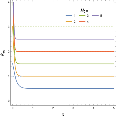
(a) Comparative study of $\kappa_{sg}$ with time for usual case (dotted line) and modified case (solid line) for $k=0$ using exponential scale factor $H_{0}=1,2,3,4,5$

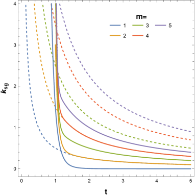
(b) Comparative study of $k_{sg}$ with time for usual case (dotted line) and modified case (solid line) for $k=0$ using power law scale factor $m=1,2,3,4,5$

Figure 1: Variation $k_{sg}$ with time for $k=0$

Figure (1(a)) illustrates the comparison of the time-dependent behavior of the $\kappa_{sg}$ parameter between the standard $f(R,T)$ gravity and a non-canonical (K-essence) $f(\bar{R},\bar{T})$ gravity scenario, both with $\kappa=0$, using the exponential scale factor (34). Typically, surface gravity diminishes with time, beginning from a larger magnitude and eventually reaching a constant value. In our scenario, the parameter $k_{sg}$ exhibits comparable fluctuations i.e., at the initial time ($t\approx 0$), the value of $k_{sg}$ undergoes a rapid change.

On the other hand, Fig. (1(b)) represents the $\kappa_{sg}$ vs. time plot using the power law scaling factor (35). In addition to the initial value, there is also a disparity in stiffness over the early period. Typically, the decrease of $k_{sg}$ is less in the unmodified case compared to the modified case. The values of $k_{sg}$ for each $m$ value are lower than in the ordinary scenario. The initial conditions of the two situations also vary. The value of $k_{sg}$ is missing at an early period ($t\simeq 0$) for the modified instance, yet the graphs have nearly the same characteristics. In this figure, we can see that at the time $t\approx 1$, there is a sudden decrease in surface gravity, like a step function for the modified case. The surface gravity decreases abruptly at the apparent horizon due to the expansion rate of the cosmos, which may cause distances to rise at a rate that opposes the local gravitational force. This event might have happened because the usual gravitational spacetime and the scalar (matter) field are coupled in our scenario. This may cause a sudden change in the surface gravity around the time $t\simeq 1$.

Near $t=0$, the variable $k_{sg}$ has a finite positive value in typical scenarios. However, in our specific case, no finite value has been attained for $k_{sg}$ in the two figures mentioned above. If we consider $t\simeq 0$ as the starting point of the universe (Big Bang), it is not possible to assign a definite value to it at that moment. At that time, we cannot determine the exact temperature associated with surface gravity, possibly due to significant fluctuations. However, the study of temperature fluctuation is beyond the scope of this article. In a different context, Gangopadhyay [86] evaluates the temperature fluctuations in the early universe using the K-essence model.

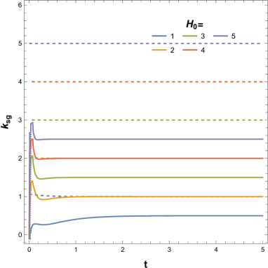
(a) Comparative study of $\kappa_{sg}$ with time for usual case (dotted line) and modified case (solid line) for $k=1$ using exponential scale factor $H_{0}=1,2,3,4,5$

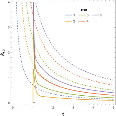
(b) Comparative study of $\kappa_{sg}$ with time for usual case (dotted line) and modified case (solid line) for $k=1$ using power law scale factor $m=1,2,3,4,5$

Figure 2: Variation $\kappa_{sg}$ with time for $\kappa=1$

Figure (2(a)) represents a comparison of the surface gravity $(k_{sg})$ for positive curvature and exponential scale factor (Eq. 34). In the usual case, the value of $k_{sg}$ has a constant behavior. In the modified case, the value of $k_{sg}$ starts after $t=0$, and then it shows some fluctuation as similar in the case of Fig. (1(a)), then it comes to a constant value. Figure (2(b)) represents the same for the power law scale factor (Eq.35). However, the nature of the usual and modified cases remains the same in this case but as before the stiffness varies. Also, the discrepancy persists at an early time. The sudden drop in $k_{sg}$ exists in this case too resulting in a step function-like behavior in Fig. (2(b)).

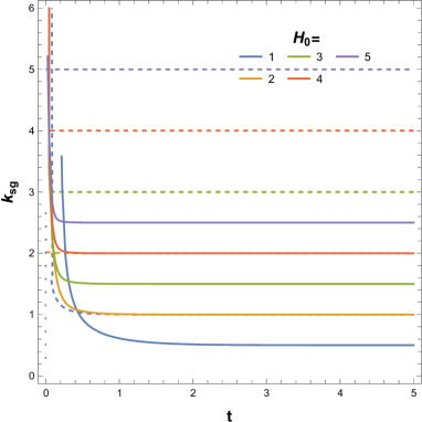
(a) Comparative study of $\kappa_{sg}$ with time for usual case (dotted line) and modified case (solid line) for $k=-1$ using exponential scale factor $H_{0}=1,2,3,4,5$

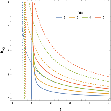
(b) Comparative study of $k_{sg}$ with time for usual case (dotted line) and modified case (solid line) for $k=-1$ using power law scale factor $m=1,2,3,4,5$

Figure 3: Variation $k_{sg}$ with time for $k=-1$

Figure (3(a)) represents the comparative study of $k_{sg}$ for negative curvature ($k=-1$) for exponential scale factor (Eq.34). For this case the behaviour of the two graphs is similar. There is a shift in the time scale only. Fig. (3(b)) represents the same for the power law scale factor (Eq.35). The value of $k_{sg}$ of the modified case is lower than the usual case in both the Figs. (3(a) and 3(b)). The unusual behavior at the early time shown in our case may be the indication of fluctuation due to the scalar field [65]. Due to the presence of this fluctuation in the physical parameter may arise in scalar field cosmology.

The Bekenstein-Hawking relation [39, 40, 41] $S_{h}=A/4G$ in GR gives the horizon entropy, where $A=4\pi\tilde{r}_{A}^{2}$ is the apparent horizon’s area. Wald [61] proposed that the entropy of black hole solutions with bifurcate Killing horizons may be understood as a Noether charge entropy within the framework of modified gravity theories. It is determined by how the modified gravitational theories’ Lagrangian density evolves with respect to the Riemann tensor. In terms of effective gravitational coupling, a quarter of the horizon area is equivalent to Wald entropy, i.e., $S_{h}=A/4G_{eff}$ [69, 70]. Following [54], in our $f(\bar{R},\bar{T})$ gravity the Wald entropy can be expressed as

$$S_{h}=\frac{Af_{\bar{R}}}{4G\mathcal{F}}=\frac{Af_{\bar{R}}}{4G+\frac{f_{\bar{T}}}{2\pi}}.$$ (37)

Taking the derivative of Eq. (32) and using (37) we get

$$d\tilde{r}_{A}=\frac{H\tilde{r}_{A}^{3}}{1-\dot{\phi}^{2}}4\pi G\frac{\mathcal{F}}{f_{\bar{R}}}\Big{[}(1-\dot{\phi}^{2})(1-2\dot{\phi}^{2})\bar{\rho}_{tot}+(1-\dot{\phi}^{2})\bar{p}_{tot}\Big{]}dt+3H\tilde{r}_{A}\dot{\phi}^{2}dt,$$ (38)

where $\bar{\rho}_{tot}=\bar{\rho}+\bar{\rho}_{d}$ and $\bar{p}_{tot}=-\bar{p}+\bar{p}_{d}$.

The small variation in the apparent horizon’s radius during a given time interval $dt$ is denoted as $d\tilde{r}_{A}$. Using (37) and (38) we can write

$$\frac{dS_{h}}{2\pi\tilde{r}_{A}}= \frac{4\pi\tilde{r}_{A}^{3}}{1-\dot{\phi}^{2}}\Bigg{[}\Big{[}(1-\dot{\phi}^{2})(1-2\dot{\phi}^{2})\bar{\rho}_{tot}+(1-\dot{\phi}^{2})\bar{p}_{tot}+\frac{3\dot{\phi}^{2}f_{\bar{R}}}{4\pi G\tilde{r}_{A}^{2}\mathcal{F}}\Big{]}Hdt+\frac{\tilde{r}_{A}f_{\bar{R}}}{2G}d\Big{(}\frac{1}{\mathcal{F}}\Big{)}+\frac{\tilde{r}_{A}}{2G\mathcal{F}}df_{\bar{R}}\Bigg{]}.$$ (39)

It follows that if we multiply the two sides of this equation by a factor ($1-\frac{\dot{\tilde{r}}_{A}}{2H\tilde{r}_{A}}$), we have

$$T_{h}dS_{h} =\frac{4\pi\tilde{r}_{A}^{3}}{1-\dot{\phi}^{2}}\Big{[}(1-\dot{\phi}^{2})(1-2\dot{\phi}^{2})\bar{\rho}_{tot}+(1-\dot{\phi}^{2})\bar{p}_{tot}+\frac{3\dot{\phi}^{2}}{f_{\bar{R}}}{4\pi}G\tilde{r}_{A}^{2}\mathcal{F}\Big{]}Hdt$$

$$-\frac{2\pi\tilde{r}_{A}^{2}}{1-\dot{\phi}^{2}}\Big{[}(1-\dot{\phi}^{2})(1-2\dot{\phi}^{2})\bar{\rho}_{tot}+(1-\dot{\phi}^{2})\bar{p}_{tot}+\frac{3\dot{\phi}^{2}}{f_{\bar{R}}}{4\pi}G\tilde{r}_{A}^{2}\mathcal{F}\Big{]}d\tilde{r}_{A}+\frac{r_{A}^{2}f_{\bar{R}}\pi}{G}T_{h}d(\frac{1}{\mathcal{F}})+\frac{\pi\tilde{r}_{A}^{2}T_{h}}{G\mathcal{F}}df_{\bar{R}}.$$

We now characterize cosmic energy inside the apparent horizon. The total matter-energy within a sphere is represented by the Misner-Sharp energy [71, 72, 56, 57, 58] in the FLRW universe, a model of a homogeneous and isotropic expanding or contracting universe. This energy might be thought of as the edge of the finite area under consideration. When the energy is projected into the universe’s apparent horizon, it obeys the unified first law of thermodynamics. In a similar manner as [54], the Misner-Sharp energy [71, 72, 73, 75] can be defined in $f(\bar{R},\bar{T})$ gravity as

$$E=\frac{\tilde{r}_{A}}{2G_{eff}}.$$ (41)

Considering the volume element $V=\frac{4}{3}\pi\tilde{r}_{A}^{3}$ and using Eqs. (25) and (32) the energy (41) can be re-written as

$$E=\frac{3V}{4\pi\tilde{r}_{A}^{2}}\frac{1}{2G_{eff}}=V\bar{\rho}_{tot}.$$ (42)

It stands for the total energy contained within the sphere of radius $\tilde{r}_{A}$. Just like in the case of regular $f(R,T)$ gravity [54], in order for the energy to be positive ($E>0$), it is necessary for the effective coupling constant $G_{eff}=\frac{G\mathcal{F}}{f_{\bar{R}}}$ to be positive, which is also true in this case. The only difference in this case is the term $f_{\bar{R}}$ is defined in the context of the K-essence $f(\bar{R},\bar{T})$ geometry.

From (26) and (42) it can be written

$$dE =4\pi\tilde{r}_{A}^{2}\bar{\rho}_{tot}d\tilde{r}_{A}+\frac{\tilde{r}_{A}(1-\dot{\phi}^{2})}{2G\mathcal{F}}df_{\bar{R}}+\frac{\tilde{r}_{A}(1-\dot{\phi}^{2})f_{\bar{R}}}{2G}d(\frac{1}{\mathcal{F}})$$ (43)

$$-\Big{[}4\pi\tilde{r}_{A}^{3}H\Big{(}(1-2\dot{\phi}^{2})\bar{\rho}_{tot}+\bar{p}_{tot}\Big{)}+\frac{\tilde{r}_{A}^{3}}{2G_{eff}}\Big{(}\frac{6k}{a^{2}}\dot{\phi}^{2}(1-\dot{\phi}^{2})-6H^{2}\dot{\phi}^{2}\Big{)}\Big{]}dt$$

Using (43) in (LABEL:40) we can write

$$(1-\dot{\phi}^{2})T_{h}dS_{h}=-dE^{\prime}+W^{\prime}dV+\frac{\tilde{r}_{A}}{2G\mathcal{F}}(1-\dot{\phi}^{2})\Big{[}1+2\pi\tilde{r}_{A}T_{h}\Big{]}df_{\bar{R}}+\frac{\tilde{r}_{A}(1-\dot{\phi}^{2})f_{\bar{R}}}{2G}\Big{[}1+2\pi\tilde{r}_{A}T_{h}\Big{]}d\Big{(}\frac{1}{\mathcal{F}}\Big{)},$$ (44)

where

$$dE^{\prime}=dE-\dot{\phi}^{2}\Big{[}4\pi H\tilde{r}_{A}^{3}\Big{(}(1-2\dot{\phi}^{2})\bar{\rho}_{tot}-\bar{p}_{tot}\Big{)}+\frac{3\tilde{r}_{A}^{2}H}{G_{eff}}+\frac{\tilde{r}_{A}^{3}}{3G_{eff}}\Big{(}\frac{k}{a^{2}}(1-\dot{\phi}^{2})-H^{2}\Big{)}\Big{]}dt$$ (45)

and work density [69, 54]

$$W^{\prime}=W+\dot{\phi}^{2}\Big{[}2\pi\tilde{r}_{A}^{2}(3\bar{\rho}_{tot}+\bar{p}_{tot})+\frac{3}{G_{eff}}\Big{]}d\tilde{r}_{A}$$ (46)

with $W=\frac{1}{2}(\bar{\rho}_{tot}-\bar{p}_{tot})$.

Equation (44) can be expressed in a compact form

$$(1-\dot{\phi}^{2})T_{h}dS_{h}+(1-\dot{\phi}^{2})T_{h}d_{j}S_{h}=-dE^{\prime}+W^{\prime}dV$$ (47)

where

$$d_{j}S_{h}=-\frac{\tilde{r}_{A}}{2GT_{h}}\Big{[}1+2\pi\tilde{r}_{A}T_{h}\Big{]}d\Big{(}\frac{f_{\bar{R}}}{\mathcal{F}}\Big{)}=-\frac{\mathcal{F}(E+S_{h}T_{h})}{T_{h}f_{\bar{R}}}d\Big{(}\frac{f_{\bar{R}}}{\mathcal{F}}\Big{)}.$$ (48)

On comparison with GR, Gauss-Bonnet gravity, and Lovelock gravity [48, 76, 50] the usual $f(R,T)$ gravity produces the extra entropy production term $d_{j}S_{h}$ [54] due to the coupling, which has been modified in our geometry through the modified $f_{\bar{R}}$ and $f_{\bar{T}}$ terms.

IV.2 Generalized second law of thermodynamics in $f(\bar{R},\bar{T})$ gravity

According to [54, 74, 75] the generalized second law of thermodynamics (GSLT) can be expressed as

$$\dot{S}_{h}+d_{j}\dot{S}_{h}+\dot{S}_{tot}\geq 0,$$ (49)

where $S_{h}$ is the horizon entropy, $d_{j}\dot{S}_{h}=\partial_{t}(d_{j}S_{h})$ and $S_{tot}$ is the total entropy resulting from all the matter and energy sources inside the horizon in the modified $f(\bar{R},\bar{T})$ gravity. In [75, 77], it is noted that ordinary matter can be seen as a representation of a mixture of fields. These fields can be in a pure state or not and they have their own entropy. With the inclusion of other matter fields and energy components (e.g. interactive fields or energy), the total temperature $T_{tot}$ along with the total entropy $(S_{tot})$ gives

$$T_{tot}dS_{tot}=d(\bar{\rho}_{tot}V)+\bar{p}_{tot}dV,$$ (50)

which is Gibb’s equation for the fluid of matter (scalar fields) and energy [77]. Within the horizon, $T_{tot}$ represents the temperature as a whole. Here, we expressed the above Gibb’s equation in the context of K-essence $f(\bar{R},\bar{T})$ gravity such that when we withdraw the coupling factor, i.e., if we consider non-interaction between gravity and scalar fields, we get back to the original Gibb’s equation stated in [54, 75, 77]. The temperature of the apparent horizon is assumed to be proportional to $T_{tot}$ [75, 49] i.e., $T_{tot}=bT_{h}$, where $0<b<1$, to guarantee that the temperature is both below the horizon and positive. Using (45) and (50) in (49) we get

$$\dot{S}_{h}+d_{j}\dot{S}_{h}+\dot{S}_{tot}=\frac{24\pi\Xi}{\tilde{r}_{A}b\mathcal{R}}\geq 0$$ (51)

where

$$\Xi =\frac{\bar{\rho}_{tot}\dot{V}}{1-\dot{\phi}^{2}}\Big{[}1-\frac{b}{2}+\dot{\phi}^{2}(b-1)\Big{]}+\frac{V\dot{\bar{\rho}}_{tot}}{(1-\dot{\phi}^{2})}(1-b+\dot{\phi}^{2})+\frac{\bar{p}_{tot}\dot{V}}{(1-\dot{\phi}^{2})}(1-\frac{b}{2}-\dot{\phi}^{2})$$ (52)

$$+\frac{4\pi\tilde{r}_{A}^{3}b\dot{\phi}^{2}}{(1-\dot{\phi}^{2})}\Big{[}2\pi\tilde{r}_{A}(3\bar{\rho}_{tot}+\bar{p}_{tot})+\frac{1}{G_{eff}}\Big{]}\dot{\tilde{r}}_{A}$$

and

$$\mathcal{R}=\bar{R}-\frac{18\dot{\phi}^{2}H}{(1-\dot{\phi}^{2})}\Big{(}H+\frac{\sqrt{a^{2}-k\tilde{r}_{A}^{2}}}{a^{2}\tilde{r}_{A}}\Big{)}+\frac{12k}{a^{2}}.$$ (53)

The additional interaction terms due to the presence of $\dot{\phi}^{2}$ modify the GSLT (51) in our case. If we consider $\dot{\phi}^{2}=0$ we would eventually get back the usual GSLT in the usual $f(R,T)$ gravity  [54]. We expressed the terms in Eqs. (51) and (52) in a manner that makes the GSLT for our instance look like the structure suggested in [54]. However, the underlying geometry greatly differs between the two situations, which should result in additional characteristics beyond the ordinary case.

V Study of Entropy

In this part, we want to demonstrate the validity of GSLT (49) or (51).

Let us denote the rate of change of entropy for horizon entropy ($\dot{S}_{h}$), entropy from inside the horizon ($\dot{S}_{tot}$) and extra entropy coming from interaction ($d_{j}\dot{S}_{h}$) as a sum

$$\dot{S}=\dot{S}_{h}+d_{j}\dot{S}_{h}+\dot{S}_{tot}.$$ (54)

According to the generalized second law of thermodynamics (GSLT) this term should be greater than zero [75, 54]. To check this in our context we calculate the terms $\Xi,\leavevmode\nobreak\ \mathcal{R}$ in Eq.s (52) and (53) respectively. Using (25) and (26) we can find out $\bar{\rho}_{tot},\leavevmode\nobreak\ \dot{\bar{\rho}}_{tot}\leavevmode\nobreak\ \text{and}\leavevmode\nobreak\ \bar{p}_{tot}$. $\dot{V}$ can be calculated as $4\pi\tilde{r}_{A}^{2}\dot{\tilde{r}}_{A}$. The value of $\tilde{r}_{A}$ and $\dot{\tilde{r}}_{A}$ can be formulated from Eq. (32). Now we have to choose a particular function of $f(\bar{R},\bar{T})$. We decide to take it as Starobinsky type function [78, 79, 33] which says

$$f(\bar{R},\bar{T})=\bar{R}+\alpha\bar{R}^{2}+\lambda\bar{T}$$ (55)

where $\alpha$ and $\lambda$ are constants.

Also, consider that the scalar field behaves as [35, 33]

$$\dot{\phi}^{2}=e^{-t/\tau}$$ (56)

where $\tau$ is a positive constant, maintaining the conditions imposed on $\dot{\phi}^{2}$ as $0<\dot{\phi}^{2}<1$.

The relationship between the scale factor ($a(t)$) and the scalar filed ($\phi$) in Eq. (20) has also been used to derive

$$a(t)=\Big{(}\frac{1-\dot{\phi}^{2}}{\dot{\phi}^{2}}\Big{)}^{1/6}.$$ (57)

V.1 Variation of $\dot{S}$

Using Eqs. (55), (56) and (57), we derive from (51)

$$\dot{S}=\frac{N}{D},$$ (58)

where the expression of the numerator (N) and the denominator (D) has been expressed in (59) and (60) in Appendix A VI.

Now let’s plot this function ($\dot{S}$) with respect to the cosmic time ($t$) for some particular choices of parameters ($\alpha,\leavevmode\nobreak\ \lambda,\leavevmode\nobreak\ \tau,\leavevmode\nobreak\ \text{and}\leavevmode\nobreak\ b$). We take the positive ($k=1$), zero ($k=0$) and negative curvature ($k=-1$) values in each graph. The values of $\alpha$ and $\lambda$ are set to $1$ for simplicity.

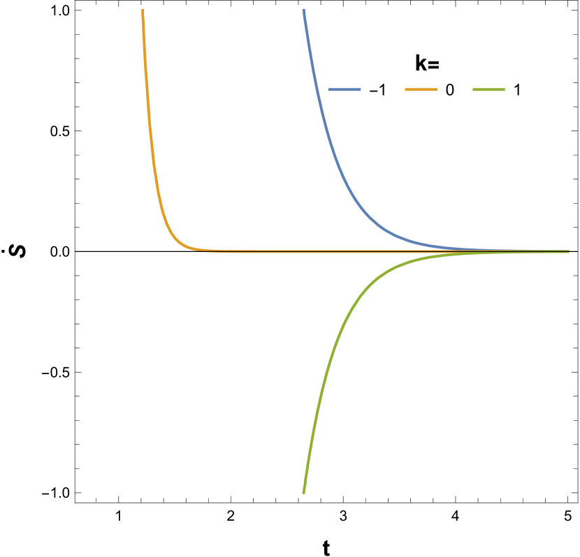
(a) Variation of $\dot{S}$ with $t$ for $\alpha=1,\leavevmode\nobreak\ \lambda=1,\leavevmode\nobreak\ \tau=0.1,\leavevmode\nobreak\ b=0.1$

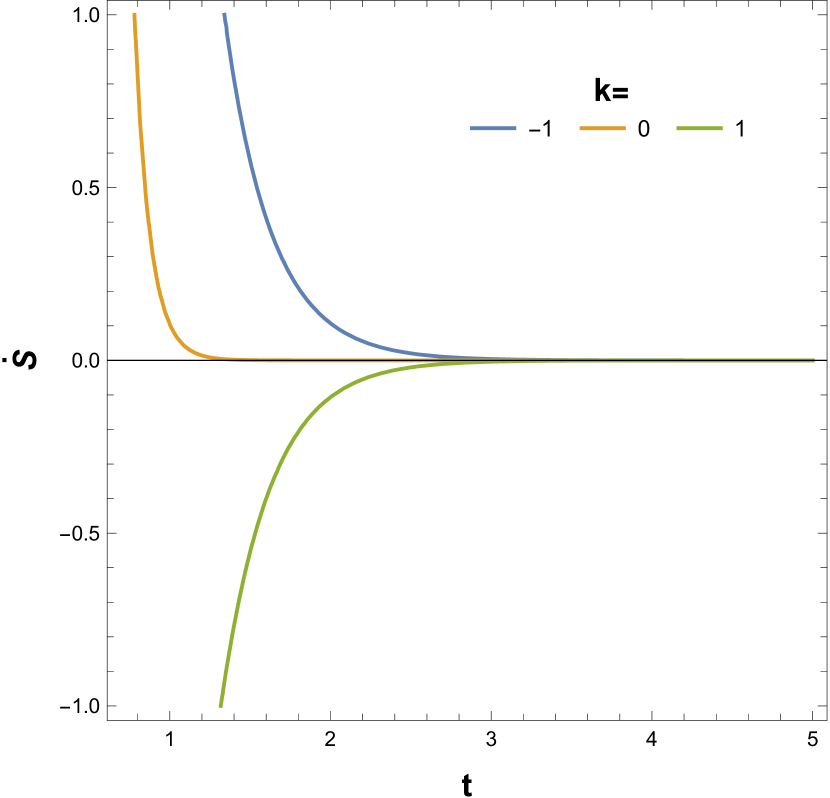
(b) Variation of $\dot{S}$ with $t$ for $\alpha=1,\leavevmode\nobreak\ \lambda=1,\leavevmode\nobreak\ \tau=0.1,\leavevmode\nobreak\ b=0.9$

Figure 4: Variation of $\dot{S}$ with $t$

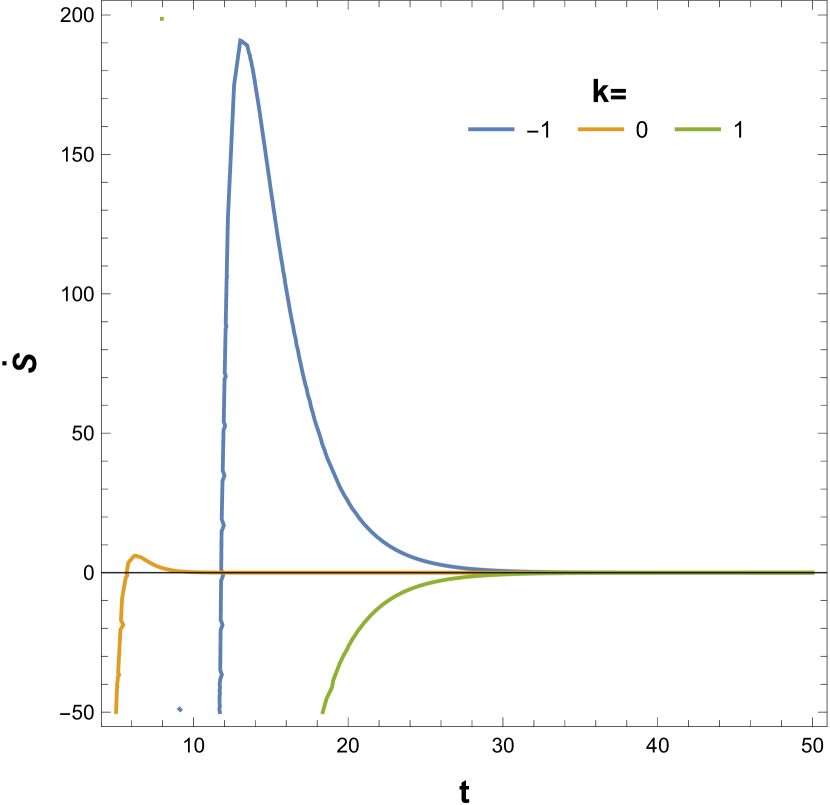
(a) Variation of $\dot{S}$ with $t$ for $\alpha=1,\leavevmode\nobreak\ \lambda=1,\leavevmode\nobreak\ \tau=0.9,\leavevmode\nobreak\ b=0.1$

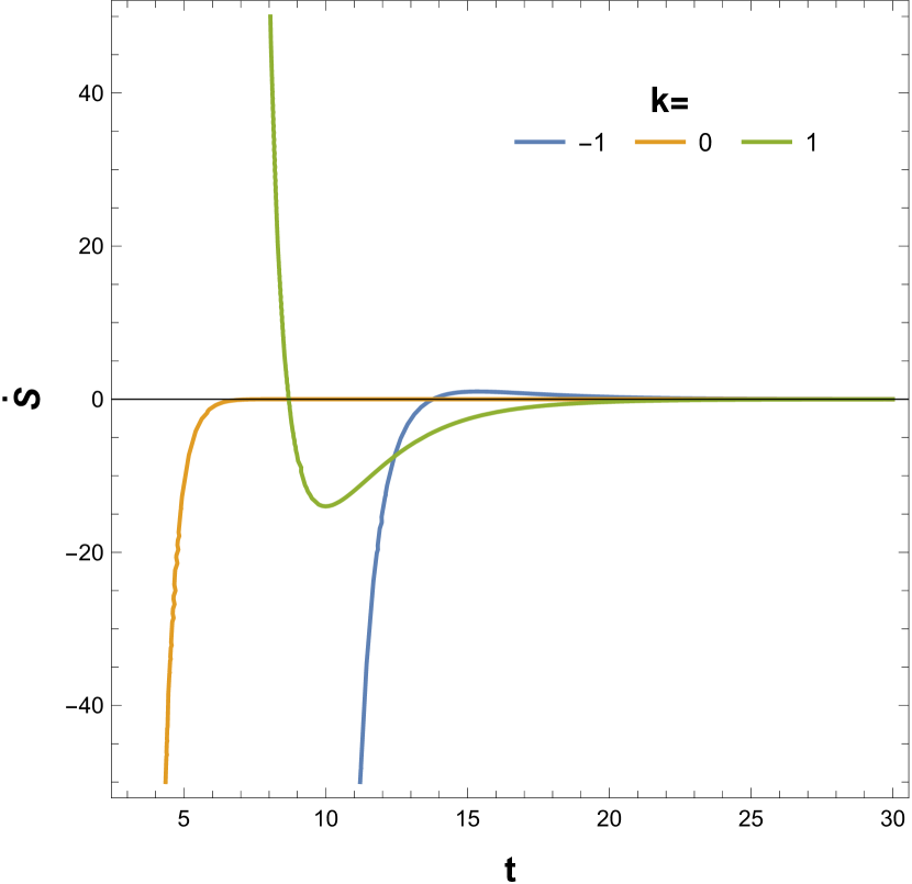
(b) Variation of $\dot{S}$ with $t$ for $\alpha=1,\leavevmode\nobreak\ \lambda=1,\leavevmode\nobreak\ \tau=0.9,\leavevmode\nobreak\ b=0.9$

Figure 5: Variation of $\dot{S}$ with $t$

Figure (4(a)) represents the variation of $\dot{S}$ with time ($t$) for $\tau=0.1$ and $b=0.9$. This graph shows negative behavior at first, then it becomes constant at $t=0$ for $k=1$. For $k=0\leavevmode\nobreak\ \&\leavevmode\nobreak\ -1$, $\dot{S}$ is always positive. Fig. (4(b)) which has been plotted for $(\dot{S})$ with $\alpha=1,\leavevmode\nobreak\ \lambda=1,\leavevmode\nobreak\ \tau=0.1\leavevmode\nobreak\ \&\leavevmode\nobreak\ b=0.9$ shows the similar type of behavior. For all the cases of $k=-1,0,1$, $\dot{S}$ becomes constant at zero after a time interval, indicating the universe’s constant entropy. In comparison with Figs. (4(a)) and (4(b)) we get to see that when $b$ is greater, the entropy becomes constant at an earlier stage of time. From these two graphs, it may be said that the universe with positive curvature seems irrelevant in the context of thermodynamics. The greater value of $b(\to 1)$ means the horizon temperature and the total temperature become almost equal, which means the energy distribution is at the end, therefore the saturation in entropy is evident.

Figure (5(a)) depicts the relationship between the rate of change of entropy ($\dot{S}$) and time ($t$) with a value of $\tau$ equal to 0.9 and $b$ equal to 0.1. The variation of $\dot{S}$, first exhibits a significantly negative value, then rises and attains a positive value, and eventually reaches zero at different times for different values of $k$. When $k=-1$, there is a prominent positive peak at the beginning of the time period. In all instances, it converges to zero after a certain period of time. The reliability of GSLT was compromised during the first stages of its development. This implies that the larger value of $\tau$ has distinct physical implications for the validity of the GSLT. Figure (5(b)) represents the same for $\tau=0.9$ and $b=0.9$. Here, $\dot{S}$ shows similar behavior as of Fig. (5(a)) for $k=0\leavevmode\nobreak\ \&\leavevmode\nobreak\ -1$, But for $k=1$, $\dot{S}$ starts from a positive value, then after reaching a negative minima (at $t\approx 10$) it becomes zero.

The above graph analysis using the GSLT (49) exhibited some differences in how the rate of change of entropy ($\dot{S}$) behaved near the beginning of the universe. These differences can be explained below:

The GSLT states that a homogeneous and isotropic system (such as the entire universe) will always grow in entropy. This rule allows for local or temporary subsystem entropy reductions. Entropy increases generally in the cosmos, although particular components may decrease. For an example of a local system, when water freezes to ice, its entropy falls because it has fewer configurations. The emission of heat during this process increases the universe’s entropy more than water’s. Thus, negative entropy changes in specific regions do not violate the Second Law because other processes compensate for them. We may say that understanding these changes in entropy is crucial in cosmology, since it enables us to accurately simulate the progression of the cosmos, including phase transitions, particle generation, and energy transfer. Also, it may emphasize the complex interaction of thermodynamics, gravitation, and cosmic development. Recall that entropy is a measure of disorder or unpredictability in the cosmos, and its behavior may reflect the intricate dynamics of numerous physical processes. In the case of our study, this phenomenon may arise from the presence of an interaction between normal gravity and a scalar field, resulting in the existence of negative entropy rates. The negative nature of $\dot{S}$ has been achieved in various articles, e.g., in the case of the quintessence field [80], in $f(T)$ gravity [81] and in the scalar field (phantom) [82]. The universe started with a very high or low entropy. If we consider the cosmic microwave background (CMB), which represents a homogeneous, isotropic, isothermal, isobaric, iso-everything universe, the entropy should be maximum. But if so, then how does the universe proceed further? The entropy should then start at a lower value [84]. As time evolves, the availability of phase space increases tremendously due to inflation, and the entropy or disorderliness increase [83]. After inflation, the rate of expansion decreases until accelerated expansion comes into play. In our graphs, we also see a sharp variation in the early stages of time, which may be the indication of the rigorous change of entropy as stated in [83]. Again according to [84] if every source of free energy in the universe has already been found, the universe will eventually go to “heat death”, dissipate all of its free energy, and become less and less complex due to the universe’s expansion speeding up and approaching a vacuum state leaving the universe with constant entropy ($\dot{S}=0$). This has also been observed in our graphs of $\dot{S}$.

VI Conclusion

This article investigates the thermodynamic properties of a homogeneous and isotropic universe using the FLRW model in modified $f(\bar{R},\bar{T})$ gravity within the K-essence geometry. The results differ significantly from those obtained using conventional $f(R,T)$ gravity in the usual FLRW universe framework.

From the field equations of $f(\bar{R},\bar{T})$ gravity we expressed the semi-conservation equation of this theory in Eq. (30) where the total energy exchange term ($\bar{q}_{tot}$) has been changed significantly from the usual $f(R,T)$ case due to the presence of $\dot{\phi}^{2}$. Thermodynamic variables such as radius of the apparent horizon ($\tilde{r}_{A}$) in Eq. (32) and surface gravity ($k_{sg}$) in Eq. (33) has also been modified in our case of $f(\bar{R},\bar{T})$ gravity. From the graphs (Fig.s 1-3) it is evident that the surface gravity in modified FLRW via $f(\bar{R},\bar{T})$ gravity has distinct features from that of the usual FLRW-based $f(R,T)$ gravity. We get sharp variations of $k_{sg}$ at the early time ($t\approx 0$) for exponential scale factor (Eq. 34) over the constant $k_{sg}$ in the usual case (Figs. 1(a) – 3(a)). This may be the effect of the scalar field perturbation at the time of inflation. For power law scale factor (35) the variation of $k_{sg}$ in the usual case and modified case shows a similar decreasing nature, but smoothness in the usual case is not present in our case (Figs. 1(b) – 3(b)). Firstly, at the initial time ($t<1$) we have not achieved any value of $k_{sg}$ whereas in usual case there exist a definite positive value of $k_{sg}$. Secondly, the value of $k_{sg}$ has a sharp decrease at the starting point, which may be an indication of the presence of fluctuation at an early time.

The first law of thermodynamics and the GSLT hold the form of Eqs. (47) and (51) respectively. The components in expressions such as Wald entropy ($S_{h}$), total energy ($E$), work function ($W^{\prime}$), extra entropy $(d_{j}S_{h})$, $\Xi$, and $\mathcal{R}$ have different forms from the usual case of $f(R,T)$. For example, to verify the GSLT, considering the Starobinsky type functional form of $f(\bar{R},\bar{T})$ and exponential form of $\dot{\phi}^{2}$, we plotted the variation of entropy ($\dot{S}$) with cosmological time ($t$) (Figs. 4 and 5). The plots show the validity or non-validity of GSLT in the context of modified $f(\bar{R},\bar{T})$ gravity. The change in entropy of the early universe may be positive or negative, subject to the value of curvature ($k=-1,0\leavevmode\nobreak\ \text{or}\leavevmode\nobreak\ 1$). The negative range of $\dot{S}$ may seem like a violation of the GSLT, but this may happen in local case scenarios. The change in entropy also shows an increasing or decreasing nature as time evolves, depending on the different curvatures of the universe. All of the plots suggest that the entropy of the universe should come to a saturation point at a later time, which leads to the entropy variation decreasing to zero. Also, the greater value of the co-efficient $b$ promotes entropy saturation at an earlier time. Note that, $b$ is the coefficient that relates the total temperature $(T_{tot})$ to the horizon temperature ($T_{h}$).

This investigation presents intriguing features regarding the thermodynamic variables and the validity of the GSLT with regard to the early cosmos. The study of the thermal properties of the cosmos within the context of modified $f(\bar{R},\bar{T})$ gravity, which is an interacting model, may provide a new avenue to understand the present scenario of the universe. The findings suggest that further investigation of scalar field perturbation during the early stages (inflationary scenario) of the cosmos is necessary. However, the study of scalar-field perturbations is beyond the scope of this article.

Acknowledgment: A.P. and G.M. acknowledge DSTB, Government of West Bengal, India, for financial support through Grant Nos. 856(Sanc.)/STBT-11012(26)/6/2021-ST SEC dated 3 November 2023. The research by M.K. was carried out in Southern Federal University with financial support of the Ministry of Science and Higher Education of the Russian Federation (State contract GZ0110/23-10-IF). SR sincerely thanks the facilities provided by ICARD, Pune at CCASS, GLA University, Mathura.

Conflicts of interest: The authors declare no conflicts of interest.

Data availability: There is no associated data with this article, and as such, no new data was generated or analyzed in support of this research.

Declaration of competing interest: The authors declare that they have no known competing financial interests or personal relationships that could have appeared to influence the work reported in this paper.

Declaration of generative AI in scientific writing: The authors state that they do not support the use of AI tools to analyze and extract insights from data as part of the study process.

Appendix A Representation of $\dot{S}$ in terms of $N$ and $D$

$$N =3e^{-\frac{4t}{\tau}}\pi\Big{(}12e^{t/\tau}k\tau^{2}+4e^{\frac{3t}{\tau}}k\tau^{2}-4k\tau^{2}+e^{\frac{2t}{\tau}}\Big{(}\sqrt[3]{-1+e^{t/\tau}}-12k\tau^{2}\Big{)}\Big{)}\Big{(}-b\Big{(}1-e^{-\frac{t}{\tau}}\Big{)}\Big{(}\Big{(}-2+7e^{-\frac{t}{\tau}}\Big{)}\alpha$$ (59)

$$-3e^{-\frac{3t}{\tau}}\Big{(}-1+e^{t/\tau}\Big{)}^{3}\tau^{2}\Big{)}\Big{(}-72e^{t/\tau}k\tau^{2}\Big{(}-1+e^{t/\tau}\Big{)}^{2/3}+36e^{\frac{2t}{\tau}}k\tau^{2}\Big{(}-1+e^{t/\tau}\Big{)}^{2/3}$$

$$+36k\tau^{2}\Big{(}-1+e^{t/\tau}\Big{)}^{2/3}+e^{\frac{3t}{\tau}}\Big{)}\Big{(}-2e^{-\frac{t}{\tau}}\Big{(}-3+e^{t/\tau}\Big{)}$$

$$\sqrt{\frac{\Big{(}-1+e^{t/\tau}\Big{)}^{3}\tau^{2}}{-72e^{t/\tau}k\tau^{2}\Big{(}-1+e^{t/\tau}\Big{)}^{2/3}+36e^{\frac{2t}{\tau}}k\tau^{2}\Big{(}-1+e^{t/\tau}\Big{)}^{2/3}+36k\tau^{2}\Big{(}-1+e^{t/\tau}\Big{)}^{2/3}+e^{\frac{3t}{\tau}}}}\sqrt[3]{-1+e^{t/\tau}}$$

$$+3e^{-\frac{2t}{\tau}}\tau\sqrt{\frac{e^{\frac{3t}{\tau}}\Big{(}-1+e^{t/\tau}\Big{)}^{2/3}}{108e^{t/\tau}k\tau^{2}-108e^{\frac{2t}{\tau}}k\tau^{2}-36k\tau^{2}+e^{\frac{3t}{\tau}}\Big{(}\sqrt[3]{-1+e^{t/\tau}}+36k\tau^{2}\Big{)}}}\Big{(}-1+e^{t/\tau}\Big{)}$$

$$+36\Big{(}1-e^{-\frac{t}{\tau}}\Big{)}^{3}k\tau^{2}\sqrt{\frac{\Big{(}-1+e^{t/\tau}\Big{)}^{3}\tau^{2}}{-72e^{t/\tau}k\tau^{2}\Big{(}-1+e^{t/\tau}\Big{)}^{2/3}+36e^{\frac{2t}{\tau}}k\tau^{2}\Big{(}-1+e^{t/\tau}\Big{)}^{2/3}+36k\tau^{2}\Big{(}-1+e^{t/\tau}\Big{)}^{2/3}+e^{\frac{3t}{\tau}}}}\Big{)}$$

$$\Big{(}-1+e^{t/\tau}\Big{)}^{2/3}+16(b-1)e^{-\frac{7t}{\tau}}\pi\tau\Big{(}-1944k\tau^{5}+54e^{t/\tau}k(252\tau+1)\tau^{4}-18e^{\frac{2t}{\tau}}k(252\alpha+\tau(2268\tau+17))\tau^{3}$$

$$+6e^{\frac{8t}{\tau}}k\Big{(}3\tau^{2}+2\alpha\Big{)}\tau^{2}+18e^{\frac{3t}{\tau}}\Big{(}3\tau\sqrt[3]{-1+e^{t/\tau}}+k\alpha(1080\tau-77)+3k\tau^{2}(1260\tau+13)\Big{)}\tau^{2}$$

$$-3e^{\frac{4t}{\tau}}\Big{(}(72\tau-1)\sqrt[3]{-1+e^{t/\tau}}+270k\tau^{2}(84\tau+1)+8k\alpha(1350\tau-169)\Big{)}\tau^{2}+3e^{\frac{5t}{\tau}}\Big{(}42\alpha\sqrt[3]{-1+e^{t/\tau}}$$

$$+8k\alpha\tau(1080\tau-161)+3\tau\Big{(}36\tau\sqrt[3]{-1+e^{t/\tau}}-\sqrt[3]{-1+e^{t/\tau}}+4536k\tau^{3}+50k\tau^{2}\Big{)}\Big{)}\tau+e^{\frac{7t}{\tau}}\Big{(}3\Big{(}18\tau\sqrt[3]{-1+e^{t/\tau}}$$

$$-\sqrt[3]{-1+e^{t/\tau}}+648k\tau^{3}-18k\tau^{2}\Big{)}\tau^{2}+\alpha\Big{(}36\tau\sqrt[3]{-1+e^{t/\tau}}+\sqrt[3]{-1+e^{t/\tau}}+1296k\tau^{3}+66k\tau^{2}\Big{)}\Big{)}-$$

$$e^{\frac{6t}{\tau}}\Big{(}9\Big{(}24\tau\sqrt[3]{-1+e^{t/\tau}}-\sqrt[3]{-1+e^{t/\tau}}+1512k\tau^{3}+6k\tau^{2}\Big{)}\tau^{2}+\alpha\Big{(}162\tau\sqrt[3]{-1+e^{t/\tau}}-49\sqrt[3]{-1+e^{t/\tau}}$$

$$+9720k\tau^{3}-1116k\tau^{2}\Big{)}\Big{)}\Big{)}\Big{(}-1+e^{t/\tau}\Big{)}^{11/3}+48(b-1)e^{-\frac{7t}{\tau}}\pi\tau^{2}\Big{(}9e^{t/\tau}\tau^{2}-3\tau^{2}+e^{\frac{3t}{\tau}}\Big{(}3\tau^{2}+2\alpha\Big{)}$$

$$-e^{\frac{2t}{\tau}}\Big{(}9\tau^{2}+7\alpha\Big{)}\Big{)}\Big{(}204e^{t/\tau}k\tau^{2}-180e^{\frac{2t}{\tau}}k\tau^{2}-72k\tau^{2}+e^{\frac{4t}{\tau}}\Big{(}\sqrt[3]{-1+e^{t/\tau}}+12k\tau^{2}\Big{)}-4e^{\frac{3t}{\tau}}\Big{(}\sqrt[3]{-1+e^{t/\tau}}-9k\tau^{2}\Big{)}\Big{)}$$

$$\Big{(}-1+e^{t/\tau}\Big{)}^{14/3}-48e^{-\frac{7t}{\tau}}\Big{(}b\Big{(}-2+e^{\frac{2t}{\tau}}\Big{)}+e^{t/\tau}-e^{\frac{2t}{\tau}}\Big{)}\pi\tau^{2}\Big{(}-72e^{t/\tau}k\tau^{2}\Big{(}-1+e^{t/\tau}\Big{)}^{2/3}$$

$$+36e^{\frac{2t}{\tau}}k\tau^{2}\Big{(}-1+e^{t/\tau}\Big{)}^{2/3}+36k\tau^{2}\Big{(}-1+e^{t/\tau}\Big{)}^{2/3}+e^{\frac{3t}{\tau}}\Big{)}\Big{(}9e^{t/\tau}\tau^{2}-3\tau^{2}+e^{\frac{3t}{\tau}}\Big{(}3\tau^{2}+2\alpha\Big{)}-$$

$$e^{\frac{2t}{\tau}}\Big{(}9\tau^{2}+7\alpha\Big{)}\Big{)}\Big{(}-1+e^{t/\tau}\Big{)}^{4}\Big{)}$$

$$D =b\Big{(}1-e^{-\frac{t}{\tau}}\Big{)}^{17/2}\Big{(}-1+e^{t/\tau}\Big{)}^{13/3}(\lambda+1)\tau^{9}\sqrt{\frac{\Big{(}-1+e^{t/\tau}\Big{)}^{10/3}\tau^{2}}{108e^{t/\tau}k\tau^{2}-108e^{\frac{2t}{\tau}}k\tau^{2}-36k\tau^{2}+e^{\frac{3t}{\tau}}\Big{(}\sqrt[3]{-1+e^{t/\tau}}+36k\tau^{2}\Big{)}}}$$ (60)

$$\Big{(}\frac{e^{-\frac{t}{\tau}}\Big{(}108e^{t/\tau}k\tau^{2}-108e^{\frac{2t}{\tau}}k\tau^{2}-36k\tau^{2}+e^{\frac{3t}{\tau}}\Big{(}\sqrt[3]{-1+e^{t/\tau}}+36k\tau^{2}\Big{)}\Big{)}}{\Big{(}-1+e^{t/\tau}\Big{)}^{7/3}\tau^{2}}\Big{)}^{5/2}\Big{(}\frac{e^{\frac{2t}{\tau}}\Big{(}-7+2e^{t/\tau}\Big{)}}{6\Big{(}-1+e^{t/\tau}\Big{)}^{3}\tau^{2}}+\frac{12k}{\sqrt[3]{-1+e^{t/\tau}}}$$

$$+\frac{e^{t/\tau}\sqrt{\frac{e^{\frac{3t}{\tau}}\Big{(}-1+e^{t/\tau}\Big{)}^{2/3}}{108e^{t/\tau}k\tau^{2}-108e^{\frac{2t}{\tau}}k\tau^{2}-36k\tau^{2}+e^{\frac{3t}{\tau}}\Big{(}\sqrt[3]{-1+e^{t/\tau}}+36k\tau^{2}\Big{)}}}}{2\Big{(}-1+e^{t/\tau}\Big{)}^{7/3}\tau\sqrt{\frac{\Big{(}-1+e^{t/\tau}\Big{)}^{3}\tau^{2}}{-72e^{t/\tau}k\tau^{2}\Big{(}-1+e^{t/\tau}\Big{)}^{2/3}+36e^{\frac{2t}{\tau}}k\tau^{2}\Big{(}-1+e^{t/\tau}\Big{)}^{2/3}+36k\tau^{2}\Big{(}-1+e^{t/\tau}\Big{)}^{2/3}+e^{\frac{3t}{\tau}}}}}-$$

$$\frac{e^{\frac{2t}{\tau}}}{2\Big{(}-1+e^{t/\tau}\Big{)}^{3}\tau^{2}}\Big{)}$$

References

• [1] Yoo J. and Watanabe Y., Theoretical models of dark energy, Int. Jour. Mod. Phys. D 2012, 21, 1230002.
• [2] Velten H. E. S., vom Marttens R. F. and Zimdahl W., Aspects of the cosmological β€œcoincidence problem”, Eur. Phys. J. C 2014, 74, 3160.
• [3] Supernova Cosmology Project collaboration, Perlmutter S. et al., Measurements of the Cosmological Parameters $\Omega$ and $\Lambda$ from the First Seven Supernovae at $z\geq 0.35$, Astrophys. J. 1997, 483, 565.
• [4] Hawkins E. et al., The 2dF Galaxy Redshift Survey: correlation functions, peculiar velocities and the matter density of the Universe, Mon. Not. Roy. Astron. Soc. 2003, 346, 78.
• [5] SDSS collaboration, Eisenstein D.J. et al., Detection of the baryon acoustic peak in the large-scale correlation function of SDSS luminous red galaxies, Astrophys. J. 2005, 633, 560.
• [6] Sotiriou T. P. and Faraoni V., $f(R)$ theories of gravity, Rev. of Mod. Phys. 2010, 82.
• [7] Harko T.; Lobo F. S. N.; Nojiri S. and Odintsov S. D., $f(R,T)$ gravity, Phys. Rev. D 2011, 84, 024020.
• [8] Carvalho G. A.; Lobato R. V.; Moraes P. H. R. S.; Arbail J. D. V., Marinho R. M.; Jr. Otoniel, E., and Malheiro M., Stellar equilibrium configurations of white dwarfs in the $f(R,T)$ gravity, Eur. Phys. J. C 2017, 77, 871.
• [9] Carvalho G. A.; Rocha F.; Oliveira H. O.; and Lobato R. V., General approach to the Lagrangian ambiguity in $f(R,T)$ gravity, Eur. Phys. J. C 2021, 81, 134.
• [10] Ordines T. and Carlson E., Limits on $f(R,T)$ gravity from Earth’s atmosphere, Phys. Rev. D 2019, 99, 104052.
• [11] Panda A.; Das S.; Manna G.; Ray S., Reconstruction of $f(R,T)$ gravity model via the Raychaudhuri equation, Phys. Dark Univ. 2024, 43 101397.
• [12] Panda A.; Manna G.; Ray S.; Khlopov M.; Islam Md. R., Gravitational collapse in generalized K-essence emergent Vaidya spacetime via $f(\bar{R},\bar{T})$ gravity, arXiv:2308.13574 (2023).
• [13] Armendariz-Picon C.; Mukhanov V.; Steinhardt P. J., Dynamical solution to the problem of a small cosmological constant and late-time cosmic acceleration, Phys. Rev. Lett. 2000, 85, 4438.
• [14] Armendariz-Picon C.; Damour T.; Mukhanov V.; k-Inflation, Phys. Lett. B 1999, 458, 209.
• [15] Armendariz-Picon C.; Mukhanov V.; Steinhardt P. J., Essentials of k-essence, Phys. Rev. D 2001, 63, 103510.
• [16] Scherrer R. J., Purely kinetic k-essence as unified dark matter, Phys. Rev. Lett. 2004, 93, 011301.
• [17] Chimento L. P., Extended tachyon field, Chaplygin gas, and solvable k-essence cosmologies, Phys. Rev. D 2004, 69, 123517.
• [18] Visser M.; Barcelo C.; Liberati S., Analogue models of and for gravity, Gen. Rel. Grav. 2002, 34, 1719.
• [19] Babichev E.; Mukhanov V.; Vikman A., k-Essence, superluminal propagation, causality and emergent geometry, JHEP 2008, 0802 101.
• [20] Vikman A., K-essence: Cosmology, causality and Emergent Geometry (Dissertation an der Fakultatfur Physik, Arnold Sommerfeld Center for Theoretical Physics, der Ludwig-Maximilians-Universitat Munchen, Munchen, 2007).
• [21] Mukohyama S.; Namba R.; Watanabe Y., Is the DBI scalar field as fragile as other k-essence fields?, Phys. Rev. D 2016, 94, 023514.
• [22] Gangopadhyay D.; Manna G., The Hawking temperature in the context of dark energy, Euro. Phys. Lett. 2012, 100, 49001.
• [23] Manna G.; Gangopadhyay D., The Hawking temperature in the context of dark energy for Reissner–Nordstrom and Kerr background, Eur. Phys. J. C 2014, 74 2811.
• [24] Manna G.; Majumder B., The Hawking temperature in the context of dark energy for Kerr–Newman and Kerr–Newman–AdS backgrounds, Eur. Phys. J. C 2019, 79 553.
• [25] Goldstein H., Classical Mechanics (2nd Edition, Narosa Publishing House, 2000).
• [26] Rana N. C.; Joag P. S., Classical Mechanics, (McGraw Hill Education (India) Private Limited, 1991).
• [27] Raychaudhuri A. K., Classical Mechanics: A course of Lectures, (Oxford University Press, 1983).
• [28] Born M. and Infeld L., Foundations of the new field theory, Proc. Roy. Soc. Lond A 1934, 144, 425.
• [29] Heisenberg W., On the theory of explosive showers in cosmic radiation. II, Zeit. Phys. 1939, 113, 61.
• [30] Dirac P. A. M., An extensible model of the electron, Royal Society of London Proceedings Series A 1962, 268, 57.
• [31] Dutta J.; Khyllep W.; Zonunmawia H., Cosmological dynamics of the general non-canonical scalar field models, Eur. Phys. J. C 2019, 79, 359.
• [32] De-Santiago J.; Cervantes-Cota J. L. and Wands D., Phase space analysis of the $F(X)–V(\phi)$ scalar field Lagrangian and scaling solutions in flat cosmology, Phys. Rev. D 2013, 87 023502.
• [33] Panda A.; Ray S.; Manna G.; Das S.; Ranjit C. , Cosmological effects on $f(\bar{R},\bar{T})$ gravity through a non-standard theory, Int. Jour. Mod. Phys. D, 2024, 33, 2450015;
• [34] Gangopadhyay D.; Manna G., Cosmology in presence of dark energy in an emergent gravity scenario, e-Print: 1502.06255 [gr-qc], (2015).
• [35] Manna G.; Majumdar P.; Majumder B., K-essence emergent spacetime as a generalized Vaidya geometry, Phys. Rev. D 2020, 101, 124034.
• [36] Manna G., Gravitational collapse for the K-essence emergent Vaidya spacetime, Eur. Phys. J. C 2020, 80, 813.
• [37] Majumder B., Ray S., and Manna G., Evaporation of Dynamical Horizon with the Hawking Temperature in the K‐essence Emergent Vaidya Spacetime, Fortschr. Phys., 71, 2300133, (2023)
• [38] Majumder B., Khlopov M., Ray S., and Manna G., Geodesic structure of generalized Vaidya spacetime through the K-essence, Universe, 9, 510, (2023)
• [39] Bardeen J.M.; Carter B. and Hawking S., The four laws of black hole mechanics, Commun. Math. Phys. 1973, 31, 161.
• [40] Hawking S.W., Particle Creation by Black Holes, Commun. Math. Phys.1975, 43, 199.
• [41] Bekenstein J.D., Black holes and entropy, Phys. Rev. D 1973, 7, 2333.
• [42] Jacobson T., Thermodynamics of spacetime: the Einstein equation of state, Phys. Rev. Lett. 1995, 75, 1260.
• [43] Unruh W. G., Notes on black-hole evaporation, Phys. Rev. D 1976, 14, 870.
• [44] Frolov A.V.; Kofman L., Inflation and de Sitter thermodynamics, JCAP 2003, 0305, 009.
• [45] Danielsson U.H., Transplanckian energy production and slow roll inflation, Phys. Rev. D 2005,71, 023516.
• [46] Bousso R., Cosmology and the S-matrix, Phys. Rev. D 2005, 71, 064024.
• [47] Cai R.G. and Kim S.P., Unified first law and the thermodynamics of the apparent horizon in the FRW universe, JHEP 2005, 02, 050.
• [48] Akbar M. and Cai R.G., Thermodynamic behavior of field equations for $f(R)$ gravity, Phys. Lett. B 2007, 648, 243-248.
• [49] Bamba K.; Geng C.Q. and Tsujikawa S., Equilibrium thermodynamics in modified gravitational theories, Phys. Lett. B 2010, 688, 101-109.
• [50] Cai R.G. and Cao L.M., Unified first law and the thermodynamics of the apparent horizon in the FRW universe, Phys. Rev. D 2007, 75, 064008.
• [51] Cai R.G.; Cao L.M.; Hu Y.P. and Kim S.P., Generalized Vaidya Spacetime in Lovelock Gravity and Thermodynamics on Apparent Horizon, Phys. Rev. D 2008, 78, 124012.
• [52] Sheykhi A.; Wang B. and Cai R.G., Thermodynamical properties of apparent horizon in warped DGP braneworld, Nucl. Phys. B 2007, 779, 1.
• [53] Bamba K. and Geng C.Q., Thermodynamics in f (R) gravity in the Palatini formalism, JCAP 2010, 06, 014.
• [54] Sharif M. and Zubair M., Thermodynamics in f (R, T) theory of gravity, JCAP 2012, 03, 028.
• [55] Nojiri S. and Odintsov S.D., Inhomogeneous equation of state of the universe: Phantom era, future singularity and crossing the phantom barrier, Phys. Rev. D 2005, 72, 023003.
• [56] Kodama H., Conserved energy flux for the spherically symmetric system and the backreaction problem in the black hole evaporation, Prog. of Theor. Phys., 63, 4, (1980).
• [57] Criscienzo R. D., Hayward S. A, Nadalini M, Vanzo L. and Zerbini S., Hamilton–Jacobi tunneling method for dynamical horizons in different coordinate gauges, Class. Quantum Grav. 27, 015006, (2010).
• [58] Faraoni V., Evolving Black Hole Horizons in General Relativity and Alternative Gravity, Galaxies, 2013, 1, 114-179.
• [59] Koivisto T., A note on covariant conservation of energy–momentum in modified gravities, Class. Quant. Grav. 2006, 23, 4289.
• [60] Carvalho G.A.; Rocha F; Oliveira H.O.; Lobato R.V., General approach to the Lagrangian ambiguity in $f(R,T)$ gravity, Eur. Phys. J. C 2021, 81, 134.
• [61] Wald R.M., Black hole entropy is the Noether charge, Phys. Rev. D 1993, 48, 3427.
• [62] Weinberg S., β€œCosmology”, Oxford University Press, New York, Indian Edition, 2008.
• [63] Peebles P.J.E., Principles of Physical Cosmology, Princeton University Press, 1993 (pp-396).
• [64] Liddle A. R. and Lyth D. H., Cosmological Inflation and Large-Scale Structure, Cambridge University Press, 2000, (pp-49).
• [65] Mukhanov V., Physical Foundations of Cosmology, Cambridge University Press; 2005, (Chapters 5 and 8)
• [66] Kadam S. A., Said J. L. and Mishra B., Accelerating cosmological models in f (T, B) gravitational theory, Int. Jour. Geom. Meth. Mod. Phys. 20, 05, 2350083 (2023).
• [67] Bahamonde S., Zubair M., Abbas G., Thermodynamics and cosmological reconstruction in $f(T,B)$ gravity, Phys. Dark Univ., 19, 78-90 (2018).
• [68] Ye G., Zhu M., and Cai Y., Null energy condition violation during inflation and pulsar timing array observations, J. High Energ. Phys. 2024, 8 (2024).
• [69] Hayward S.A., Unified first law of black-hole dynamics and relativistic thermodynamics, Class. Quant. Grav. 1998, 15, 3147.
• [70] Hayward S.A.; Mukohyama S. and Ashworth M., Dynamic black-hole entropy, Phys. Lett. A 1999, 256, 347.
• [71] Misner C.W. and Sharp D.H., Relativistic equations for adiabatic, spherically symmetric gravitational collapse, Phys. Rev. 1964, 136, B571.
• [72] Bak D. and Rey S.J., Cosmic holography+, Class. Quant. Grav. 2000, 17, L83.
• [73] Gong Y. and Wang A., Friedmann equations and thermodynamics of apparent horizons, Phys. Rev. Lett. 2007, 99, 211301.
• [74] Davies P C W, Cosmological horizons and the generalised second law of thermodynamics, Class. Quantum Grav. 4, L225-L228 (1987).
• [75] Wu S. F.; Wang B.; Yang G.H. and Zhang P.M., The generalized second law of thermodynamics in generalized gravity theories, Class. Quantum Grav. 2008, 25, 235018.
• [76] Cai R.G. and Cao L.M., Unified first law and the thermodynamics of the apparent horizon in the FRW universe, Phys. Rev. D 2007, 75, 064008.
• [77] Izquierdo G. and Pavon D., Dark energy and the generalized second law, Phys. Lett. B 2006, 633, 420.
• [78] Moraes P. H. R. S.; Sahoo K.; Ribeiro G. and Correa R. A. C., A Cosmological Scenario from the Starobinsky Model within the $f(R,T)$ Formalism, Advances in Astronomy 2019, 2019, 8574798.
• [79] Starobinsky A. A., Disappearing cosmological constant in $f(R)$ gravity, JETP Letters volume 2007, 86, 157–163.
• [80] Setare M.R., Generalized second law of thermodynamics in quintom dominated universe, Phys. Lett. B., 641 (2006) 130–133.
• [81] Ghosh R., Pasqua A. and Chattopadhyay S. Generalized second law of thermodynamics in the emergent universe for some viable models of f(T) gravity, Eur. Phys. J. Plus (2013) 128, 12.
• [82] Chattopadhyay S. and Debnath U., Generalized second law of thermodynamics in the presence of interacting tachyonic field and scalar (phantom) field, Can. J. Phys. 88: 933–938 (2010).
• [83] Hawking, S. W., Arrow of time in cosmology, Phys. Rev. D, 32 (10), 2489–2495 (1985).
• [84] Lineweaver CH. A simple treatment of complexity: cosmological entropic boundary conditions on increasing complexity. In: Lineweaver CH, Davies PCW, Ruse M, eds. Complexity and the Arrow of Time. Cambridge University Press; 2013, 42-67.
• [85] Penrose R. (2004), The big bang and its thermodynamic legacy. In Road to reality: a complete guide to the laws of the universe, London: Vintage Books p. 686–734 [Chapter 27].
• [86] Gangopadhyay, D. Estimating temperature fluctuations in the early universe, Gravit. Cosmol. 16, 231–238 (2010).