BlockLLM: Memory-Efficient Adaptation of LLMs by Selecting and Optimizing the Right Coordinate Blocks

Abstract

Training large language models (LLMs) for pretraining or adapting to new tasks and domains has become increasingly critical as their applications expand. However, as the model and the data sizes grow, the training process presents significant memory challenges, often requiring a prohibitive amount of GPU memory that may not be readily available. Existing methods such as low-rank adaptation (LoRA) add trainable low-rank matrix factorizations, altering the training dynamics and limiting the model’s parameter search to a low-rank subspace. GaLore, a more recent method, employs Gradient Low-Rank Projection to reduce the memory footprint, in the full parameter training setting. However GaLore can only be applied to a subset of the LLM layers that satisfy the “reversibility” property, thus limiting their applicability. In response to these challenges, we introduce BlockLLM, an approach inspired by block coordinate descent. Our method carefully selects and updates a very small subset of the trainable parameters without altering any part of its architecture and training procedure. BlockLLM achieves state-of-the-art performance in both finetuning and pretraining tasks, while reducing the memory footprint of the underlying optimization process. Our experiments demonstrate that fine-tuning with only less than 5% of the parameters, BlockLLM achieves state-of-the-art perplexity scores on the GLUE benchmarks. On Llama model pretrained on C$4$ dataset, BlockLLM is able to train with significantly less memory than the state-of-the-art, while still maintaining competitive performance.

1 Introduction

Recent advancements in natural language processing (NLP) have been propelled by the development of large language models (LLMs) [15, 30, 22, 1]. These models have set new benchmarks for a variety of NLP tasks, including language translation [29], text summarization [13], and sentiment analysis [3]. The core strength of LLMs lies in their scale. Empirical evidence suggests that increases in model size not only enhance performance across standard benchmarks but also unlock new capabilities that are absent in smaller models [12, 35]. Pre-training and finetuning LLMs on domain-specific application data have enhanced their applicability immensely.

However, pre-training and finetuning LLMs are resource-intensive processes, requiring substantial memory and computational power. For example, a $7B$ parameter Llama model demands approximately $14$GB of memory [34], assuming each parameter is a $16$-bit float occupying 2 bytes. The memory required for storing gradients during backpropagation is similarly substantial, adding another $14\text{ GB}$. Additionally, LLMs are often trained using the Adam optimizer [14] and its variants, which maintain first and second moment estimates for each parameter. This effectively doubles this memory requirement, resulting in an additional $28\text{ GB}$ of VRAM memory. Consequently, the total memory required for the weights, gradients, and optimizer states amounts to a whopping $56\text{ GB}$. The effect of LLMs training’s high memory require is far reaching, in that it comes down to the question of who can train these large models. With the memory calculations above, a $7$ billion parameter model can only be trained on A100 GPUs or above. This is a significant barrier to entry for researchers and practitioners who do not have access to such high-end hardware.

Existing strategies for memory-efficient training.

To address these challenges, multiple strategies are being explored to reduce the number of parameters, gradients, and the corresponding optimizer state size. One popular strategy is the application of pruning methods, where a large set of parameters or even entire layers are removed from the model architecture [32, 18, 28]. However, pruning approaches often require extensive retraining to recover lost accuracy [5]. Furthermore, identifying which parameters are crucial before training is challenging [20, 26]. This challenge complicates implementation and can lead to generalization issues, particularly on diverse or unseen data [18].

PEFT (Parameter-Efficient-Fine-Tuning) methods such as [9, 16, 10] achieve memory efficiency by introducing low-rank matrices to the transformer architecture, significantly reducing the number of trainable parameters needed during fine-tuning. Although integrating these low-rank matrices alleviates the extensive retraining demanded by pruning techniques, they can alter the training dynamics, potentially leading to quality issues during the merging phase [8]. Moreover, the additional parameters introduced by PEFT methods can increase the model’s parameter size, countering efforts to reduce overall model size.

A recent work, GaLore [34], which focuses on full parameter training, achieves memory efficiency by performing low-rank factorization of the gradients in specific layers. However, GaLore does not achieve high memory efficiency across all model types, as its gradient factorization method can only be applied to layers that satisfy the reversibility property. This limitation restricts its applicability and efficiency in models where not all layers exhibit this property.

Techniques such as gradient and activation checkpointing, quantization, and parameter offloading are also commonly used to achieve memory savings. These methods often come with trade-offs, such as increased computational overhead or compromised performance. For instance, checkpointing [4] reduces memory usage but requires recomputation, quantization lowers precision and can affect accuracy [7] and parameter offloading increases data transfer latency [25].

Block coordinate descent (BCD).

BCD is a popular algorithm in the large-scale optimization literature [21]. At any training iteration $t$, instead of updating all the parameters $W$, BCD selectes only a block of parameters $b_{t}$ and updates only

$$W^{b_{t}}_{t+1}=W^{b_{t}}_{t}+d_{t},$$

where $d_{t}$ is the update. As it can be seen, this formulation directly falls in the reduced parameter training regime. This insight forms the cornerstorne of our approach and hence the name BlockLLM. A related study by Belilovsky et al. [2] demonstrated that sequentially solving one-hidden-layer problems could match the performance of large model training, inspiring us to tackle parameter and memory efficiency by training large models in parts. By definition, this method doesn’t alter the model architecture in anyway. Furthermore, works such as [24, 33, 21] prove the convergence of BCD on various problem architectures; inspiring us to adapt it to large scale LLM training.

Our Contributions.

We propose a novel parameter and memory-efficient algorithm, BlockLLM where we dynamically select and train a block of parameters. BlockLLM primarily achieves memory savings by persisting optimizer states only for these selected parameters. We introduce a novel block selection criterion, for LLM training. We demonstrate the memory-efficient training and superior performance of BlockLLM on pre-training and finetuning tasks.

2 Methodology

They key idea behind BlockLLM is to select and update only a subset of parameters during training, enabling us to achieve significant memory savings. However, the criteria for selecting the “right” subset of parameters is not clear. In this section, we look at magnitude pruning as a tool to identify parameter importance, in the finetuning setting.

Magnitude Pruning.

Magnitude pruning is a widely recognized technique for reducing the parameter count in neural network models [6]. In this analysis, we use parameter magnitude as a measure of parameter importance and study the impact of training on the selected parameters. First, we trained DistilBERT [27] on the IMDb dataset [19] for sequence classification, achieving an accuracy of 92.02%. We then conducted inference on the GLUE-CoLA dataset [31] without fine-tuning, resulting in a significant drop in accuracy to $47.74\%$. This drop in performance, possibly due to domain shift, encouraged us to use this setup for our analysis.

Next, we performed magnitude pruning on the IMDb pre-trained model at various sparsity levels and fine-tuned these pruned models on the GLUE-CoLA dataset. Let $s$ denote the sparsity level, $W^{t}$ represent the model parameters at iteration $t$, and $n$ be the total number of parameters. For each parameter $w_{i}$ where $i=1,\ldots,n$, we compute $|w_{i}|$. During training, we update only $S=\text{Top}_{k}|W^{0}|$, where $k=n\times(1-s)$. The results of these experiments, detailing the relationship between sparsity and accuracy, are summarized in Table 5.

Interesting results emerged from this analysis: at $0.5$ sparsity, the model retains a high accuracy of $78.52\%$, suggesting that up to $50\%$ of parameters can be pruned with minimal performance loss. However, accuracy drops significantly at 0.7 sparsity to $67.68\%$. This suggests that there is some inductive bias that the model can leverage when finetuning on a dataset with significant domain shift, under a reduced parameter setting. However, estimating the sparsity $s$ apriori is hard, and its not clear what factors influence this.

Analysis of Weight Magnitudes.

To further understand the effects of this parameter selection strategy, we analyzed $|W|$, before and after training to understand which weights are updated more frequently and their impact on model performance. Specifically, we compared the initial weights $|W^{0}|$ and final weights $|W^{t}|$ of the model after fine-tuning on the CoLA dataset [31]. Our findings are presented in Figure 1. The histogram on the left of Figure 1 shows $|w_{i}^{t}|$ for all $i$ where $\delta_{i}>\eta$. Here, $\delta_{i}=|w_{i}^{0}-w_{i}^{t}|$ and $\eta$ is the threshold. The histogram on the right of Figure 1 plots the frequency of $\delta$ in the updates, revealing that a large percentage of the updates were minor.

Several additional insights and questions emerge from these observations. The histogram of $\delta$ indicates that most weight changes are minor, suggesting that significant updates are concentrated in a small portion of the weights. These experiments raise some pertinent questions:

1. Is it reasonable to judge the impact of a parameter during training based on its initial weight magnitude?

2. How should the appropriate sparsity level $s$ be determined before commencing training?

3. Although we observed that only a few parameters undergo significant changes during training, which specific parameters are updated during various phases of the training process?

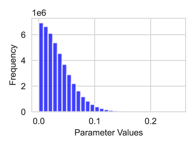
(a) Histogram of the changed parameters

(b) Histogram of $\delta$

Figure 1: Analysis of weight magnitudes of DistilBERT model pretrained on IMDb dataset and finetuned on CoLA dataset.

2.1 Analysis of Reduced Parameter Training

To address the above questions, we further investigated the pruning process. First, we updated the chosen parameter set $S$ every $m$ iterations, based on the weight magnitudes $|W^{t}|$, at current iteration $t$. This means that after every $m$, the parameter seletion criteria is revisited to obtain a new set of parameters to update. The objective is to understand if $S$ changes significantly over time and if adaptively selecting $S$ enhances the training performance. In this framework, we continue to update only the top $k=n\times(1-s)$ parameters in each iteration. However, the percentage of unique parameters $q$, updated throughout the entire training process can be greater than $(1-s)$ of $\%\$parameters updated. (i.e $q\geq 1-s$). Analysing $q$ can reveal how much parameters are truly impactful for training, thereby addressing our second question.

We conducted this experiment using the same setup: fine-tuning the DistilBERT model on the GLUE-CoLA dataset after pre-training on the IMDb dataset. The results of this experiment are summarized in the Table 1. Additionally, we performed similar experiments on other GLUE [31] datasets, with the results presented in Section A.3

$1-s$	$q$	$m$	Accuracy	Matthews Correlation
$0.1$	$0.58$	$1000$	$82.55$	$0.5882$
$0.02$	$0.36$	$1000$	$82.45$	$0.5711$
$0.02$	$0.14$	$4000$	$82.45$	$0.5794$
$0.02$	$0.10$	$6000$	$82.07$	$0.5679$

Table 1: Impact of Update Frequency and Sparsity on CoLA Dataset

Our observations indicate that $s$ decreases, meaning more parameters are updated per iteration, the number of unique parameters $q$ also increases, which results in better model performance. The increasing number of unique updates indicates that different parameters may become important at different stages of training, necessitating a more dynamic approach to parameter updates.

We also evaluated the model with varying update frequencies $m$. Naturally, as $m$ increases, the model has fewer opportunities to update a larger number of parameters, leading to a decrease in $q$. Interestingly, there is an optimal point up to which performance either improves or remains stable, beyond which it begins to decline. This suggests that updating too many parameters or too few parameters can be detrimental to the training process. These findings highlight the need for adaptive methods to determine the choice of parameters and the update frequency.

The findings from our experiments suggest that a parameter-efficient training method that updates a small set of parameters each iteration is feasible. However, some key aspects require clarification:

• Parameter Selection Criteria: Our analysis in Figure 1 indicates that the model frequently updates parameters with lower weight magnitudes. This contradicts the very premise of magnitude pruning. Therefore its not clear if adopting magnitude as a parameter importance criteria will help, in general. In our work, we bank on evidence from prior work on greedy parameter selection strategy [24, 21] and use gradient as the parameter importance criteria.

• Parameter Selection Frequency: As discussed earlier, determining when to change the set of parameters to update for a given training phase is crucial. In BlockLLM, we developed a strategy that uses the current loss objective value as a signal to decide if the parameter selection needs to be updated.

2.2 BlockLLM:

In this section we introduce BlockLLM, a parameter and memory efficient training method designed to reduce the number of trainable parameters in large language models (LLMs) without compromising training performance. Akin to other parameter-efficient fine-tuning (PEFT) methods such as LoRA [9] and ReLoRA [16], BlockLLM updates only $k$ parameters, at any iteration $t$, where $k\ll n$, $n$ is the total number of parameters. However, the main difference is that BlockLLM optimizes parameter selection by focusing on the most impactful parameters at different stages of the training process. The overall algorithm of BlockLLM is given in Algorithm 1.

Parameter Selection Criteria.

In the context of LLMs, at iteration $t$, the update to the parameter is the processed gradient $\tilde{G}_{t}$, calculated using optimizers such as Adam [14]. Specifically, for any layer $l$ of the model, the update is given by,

$$\tilde{G}^{l}_{t} =M^{l}_{t}/\sqrt{V^{l}_{t}+\epsilon}\hskip 8.5359pt\text{where,}\ M^{l}_{t}=\beta_{1}M^{l}_{t-1}+(1-\beta_{1})G_{t}^{l}\hskip 5.69046pt\text{and}\hskip 5.69046ptV^{l}_{t}=\beta_{2}V^{l}_{t-1}+(1-\beta_{2}){G_{t}^{l}}^{2}.$$ (1)

Here, $\beta_{1}$ and $\beta_{2}$ are hyperparameters of the optimizer and $G_{t}^{l}$ is the gradient at layer $l$ and $M_{t}$ and $V_{t}$ are the Bias-corrected first moment estimate and Bias-corrected second moment estimate respectievly. During the backward pass, BlockLLM selects the layers with the large $|\tilde{G}_{t}^{l}|$ and updates only those layers, denoted as set $S$. Note that by selecting full layers, we may not achieve the desired sparsity level $s$. Therefore, subsequently, for each selected layer we construct a binary mask to retain only the top $k$ parameters by gradient magnitude:

$$\text{mask}[i,j]=\begin{cases}1&\text{if }\|\tilde{G}_{t}^{l}[i,j]\|\geq\tau\\ 0&\text{otherwise},\end{cases}$$

where $\tau$ is an estimated threshold, computed by looking at the gradient values of each layer. Then, in every iteration $t$, the selected parameters in layers $l\in S$ are updated using the computed masks as:

$$W_{t+1}^{l}=W_{t}^{l}-\eta\left(\text{mask}\odot\tilde{G}_{t}^{l}\right).$$ (2)

An illustration of the proposed parameter selection procedure is given in Figure 3. However, there is one caveat with this approach. In the initial training iterations, the gradient estimates are known to be noisy. Additionally, there are several cases such as pre-training and finetuning, with heavy domain shift, where there is very little useful inductive bias. Therefore, using gradients to select important parameters may prove to be detrimental to our cause in the initial few iterations.

To address this challenge, our experiments incorporate layer visit frequency $f$ into the selection criteria. Specifically, for any layer $l\in L$, $f_{l}$ represents the z-score normalized number of times the layer has been selected. Consequently, the layer selection criterion is modified to $|\tilde{G}_{l}|/f_{l}$ which tends to select layers with high gradient norms while also considering layers that have been less frequently chosen in previous iterations. Our experimental results demonstrate that this refined selection criterion enhances performance.

Mask and Memory.

In the current implementation of BlockLLM, masks are binary matrices matching the dimensions of the gradients in their respective layers. Consequently, the memory footprint scales with the number of selected layers, as each layer requires a new mask. Therefore, for our experiments, we consider an approximation where we skip the mask computation step and update all parameters in $S$. The update step is as follows:

$$W_{t+1}=\begin{cases}W_{t}^{l}-\eta\tilde{G}_{t}^{l}&\text{if }l\in S,\\ \text{Freeze }W^{l}&\text{otherwise}.\end{cases}$$ (3)

Our experimental results demonstrate that this approximate block selection strategy is effective in practice. Nonetheless, we believe that a more refined implementation, capable of achieving a more granular parameter selection, is feasible. We reserve this as a potential area for future exploration.

Parameter Selection Frequency.

The natural next question is how many iterations to perform the update (3) with the same set $S$. BlockLLM addresses this by using the loss $\phi$ as a critical signal for determining when to change the parameter selection. Specifically, BlockLLM introduces a hyperparameter, patience $m$. At any iteration $t$, if $\phi_{t}$ exceeds the moving average of losses over the last $m$ iterations, the set $S$ is revised. The detailed parameter selection frequency algorithm is provided in in Algorithm 2.

Memory Efficiency

Next, we explore the memory benefits of training with BlockLLM, which stem primarily from its parameter-efficient training approach. In practice, updating fewer parameters directly reduces the number of gradients and optimizer states that need to be stored in VRAM. With $s\%$ sparsity, BlockLLM should directly reduce the optimizer states by $s\%$ compared to full parameter training. Our empirical analysis corroborates this.

Algorithm 1 BlockLLM Training Algorithm

1:Input: Data $X$, initial model parameters $W_{0}$,

2:sparsity $s$, set of layers $L$, learning rate $\eta$, patience parameter $m$, $\beta_{1}$, $\beta_{2}$, $\epsilon$.

3:Initialize: $M_{0}=0$, $V_{0}=0$, $H=[]$

4://Forward and backward pass

5:for each iteration $t$ do

6:     Loss $\phi_{t}$ , $G_{t}$ = Compute Gradient($W_{t}$)

7:     if (length($H$) $\geq m$ and

8:      $\phi_{t}\geq\frac{1}{m}\sum_{i=t-m+1}^{t}H[i]$) or ($t=0$) then

9:         mask, $S$ = SelectParam($G_{t}$, $s$, $L$)

10:         $H=[]$ $\triangleright$ Reset loss history

11:     end if

12:     // Update the selected params

13:     for each $l\in S$ do

14:         $G_{t}^{l}$ = Compute Gradient($W_{t}^{l}$)

15:         // Adam update as in (1)

16:         $M_{t}^{l},V_{t}^{l},\tilde{G}_{t}^{l}$ = Adam($M_{t-1}^{l},V_{t-1}^{l},G_{t}^{l}$)

17:         $\tilde{G}^{l}_{t}=\text{mask}\odot\tilde{G}_{t}^{l}$

18:         $W_{t+1}^{l}=W_{t}^{l}-\eta\tilde{G}_{t}^{l}$

19:     end for

20:end for

Algorithm 2 Select Parameters Function

1:function SelectParam($G_{t}$, $s$, $L$)

2:     Compute $\|\tilde{G}_{t}^{l}\|$ for each layer $l\in L$

3:     $n=\sum_{l\in L}\text{count}(l)$, $n_{s}=(1-s)\times n$

4:     $D\leftarrow\text{sort}(L,\text{desc},\|\tilde{G}_{t}^{l}\|/f_{l})$

5:     Initialize $S=[]$, $\Sigma_{p}=0$

6:     for each $l\in D$ do

7:         $\Sigma_{p}\mathrel{+}=\text{count}(l)$ , $S\leftarrow S\cup\{l\}$

8:         if $\Sigma_{p}\geq n_{s}$ then break

9:         end if

10:     end for

11:// Compute mask

12:     for each $l\in S$ do

13:         Let $\text{mask}_{l}$ $=\mathbf{0}_{|G_{t}^{l}|}$

14:         for each $i,j$ in mask do

15:              if $\|\tilde{G}_{t}^{l}[i,j]\|\geq\tau$ then

16:                  $\text{mask}_{l}[i,j]=1$

17:              end if

18:         end for

19:     end for

20:     return mask, $S$

21:end function

Figure 2: (Left) The main BlockLLM algorithm, (right) SELECTPARAM function that performs parameter selection at iteration $t$.

Figure 3: Given a large language model consisting of many layers, BlockLLM first finds the layers with the largest gradient $||\tilde{G}_{l}||$ (highlighted in orage) and selects a subset of the parameters. During optimization, only the selected layers will be updated ($\theta$) and the Adam optimizer will only keep track of the bias corrected moments ($M_{l}$) and ($V_{l}$) for those selected parameters (shown in orange).

3 Experiments

We evaluated BlockLLM on both finetuning tasks and pre-training tasks . The finetuning experiments were conducted in Tesla V100 gpu ($32$ GB) and the pretraining tasks were conducted on NVIDIA A40 ($48$ GB) and A100 GPUs ($80$ GB) (one GPU per experiment).

3.1 Finetuning on GLUE

The General Language Understanding Evaluation (GLUE) benchmark [31] is widely used to evaluate the performance of NLP models across a range of tasks, including sentiment analysis, question answering, and textual entailment. We benchmarked the performance of BlockLLM against GaLore [34] and full finetuning (FFT) using the pre-trained RoBERTa model [17] on GLUE tasks. We did not compare against LoRA [9] and its variants [16, 11], because our experimental setup aligns with those described in [16, 34] and the results for these methods are already documented in [34]. For BlockLLM, we conducted hyperparameter tuning for the learning rate, and our experimental setup is detailed in A.5. For GaLore, we used the learning rate specified in [34]. In our experiments, we used $s=0.95$. We evaluated both performance and memory consumption during the training process for all methods. The results, presented in Tables 2 and 3, indicate that BlockLLM outperforms the other models in all tasks while achieving approximately a 13.5% reduction in memory usage on average.

	MRPC	COLA	STS-B	RTE	SST2	MNLI	QNLI	QQP
Block-LLM	$\mathbf{3.97}$	$\mathbf{2.8}$	$\mathbf{3.48}$	$\mathbf{9.1}$	$\mathbf{3.6}$	$\mathbf{13.7}$	$\mathbf{12.8}$	$8.36$
GaLore (rank=8)	$4.52$	$4.2$	$4.8$	$9.7$	$3.87$	$15.1$	$14.8$	$8.43$
GaLore (rank=4)	$4.52$	$4.2$	$4.8$	$9.7$	$3.86$	$15.2$	$14.8$	$\mathbf{8.03}$
FFT	$4.24$	$3.67$	$4.4$	$10.28$	$3.82$	$15.53$	$15.02$	$9.22$

Table 2: VRAM Memory Comparison Across Different Tasks (measured in GB). VRAM memory usage was monitored as described in Section A.4.

	MRPC	COLA	STS-B	RTE	SST2	MNLI	QNLI	QQP
Block-LLM	91.8	$\mathbf{63.8}$	90.02	80.14	$\mathbf{94.95}$	$\mathbf{87.75}$	92.95	91.36
GaLore (rank=8)	89.96	62.5	$\mathbf{91.1}$	79.78	94.38	87.17	$\mathbf{92.97}$	91.11
GaLore (rank=4)	91.7	61.67	91.09	79.78	94.04	87	92.65	91.06
FFT	$\mathbf{92.36}$	62.84	91.1	$\mathbf{80.5}$	94.57	87.18	92.33	$\mathbf{92.28}$

Table 3: Score Comparison Across Different GLUE Tasks

3.2 Pre-training on Llama model

We also compared BlockLLM with GaLore [34] in pre-training LLaMA-based large language models [30] on the C4 (Colossal Clean Crawled Corpus) dataset [23]. The C4 dataset is a large-scale, cleaned version of the Common Crawl web corpus used for pre-training language models, featuring diverse and high-quality text from the internet. Our experiment setup is similar to [34], following the setup from [16]. We fine-tuned the learning rate for BlockLLM while keeping all other hyperparameters fixed across experiments. We ran BlockLLM with the experimental setup described in A.6 and computed the perplexity scores from final evaluation loss and maximum memory usage in GB(Gigabytes). We ran GaLore for $10\%$ of total iterations to observe memory consumption, and used the results from [34] for comparison. The perplexity and the memory are shown in the Figure 4 and Table 4.

	60M		130M		350M
	Perplexity	Memory	Perplexity	Memory	Perplexity	Memory
BlockLLM	$\mathbf{34.31}$	$\mathbf{28.27}$	$\mathbf{25.36}$	$\mathbf{40.68}$	19.02	$\mathbf{42.6}$
GaLore	34.88	32.26	$\mathbf{25.36}$	46.69	$\mathbf{18.95}$	49.06

Table 4: Comparison of Accuracy and VRAM Memory (GB) of LLama Models with GaLore. Note that for GaLore, we used AdamW as the underlying optimizer.

We note here that BlockLLM takes a little bit longer to converge for some experiments ($130m$ and $350m$ models) compared to full parameter learning methods such as GaLore in the pre-training experiment. We suspect this is due to the fact that we are dealing with noisy gradients in the earlier iterations of training. However, BlockLLM converges to the state-of-the-art perplexity score in a few more iterations compared to GaLore. This is issue is not present in the finetuning experiments.

Effect of sparsity $s$. Here, we compare BlockLLM with sparsity values $s=0.5,0.7$ and $0.9$ against full parameter training $(s=0)$ and GaLore [34]. The results are presented in Figure 4. We observe that with $s=0.5$, BlockLLM consumes about $1.5$ GB less memory than Galore and higher sparsity values further reduce memory usage though this comes with the trade-off of requiring more training iterations for similar performance.

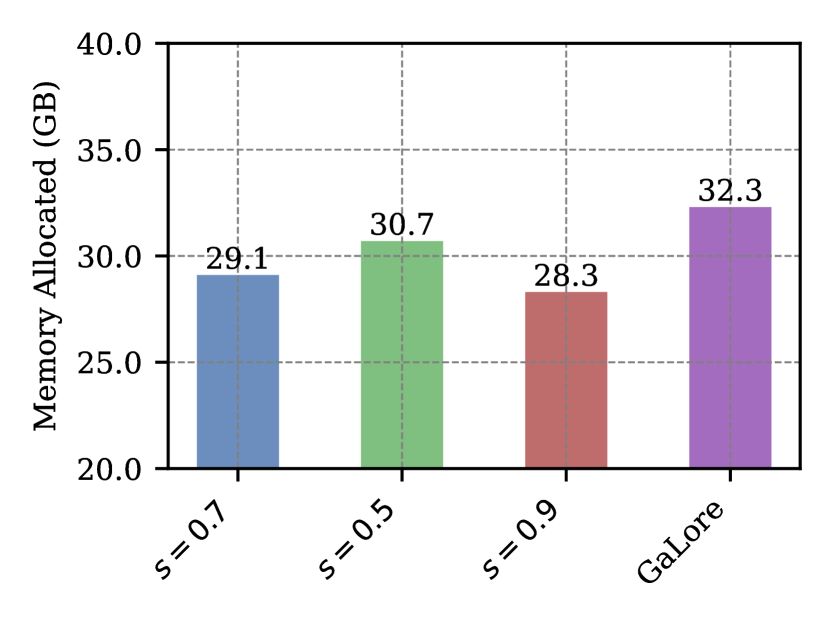
Figure 4: Comparison of perplexity (left) and memory usage (right) of Llama 60M. Here $s$ denotes the specified model sparsity. As it can be seen, BlockLLM performs competitively with GaLore, but at a much lower memory footprint.

3.3 Ablation on Parameter Selection Strategy

We investigate whether selecting parameters with higher gradient norms, which are less frequently chosen, benefits training. We observed the training performance of the LLaMA 60M model on the C4 dataset while employing the strategy of randomly selecting block parameters for updates. Specifically, let $L=[l_{1},l_{2},\dots,l_{n}]$ represent the list of all layers. At iteration $t$, we randomly select $k$ layers from $L$ with equal probability until the required number of parameters is met according to the sparsity $s$. Let $D\subseteq L_{\text{shuffled}}$ be the subset of selected layers, defined as

$$D=\{l_{i}\in L_{\text{shuffled}}:\sum_{l_{i}\in D}\text{param\_count}(l_{i})\leq s\times\sum_{l_{i}\in L}\text{param\_count}(l_{i})\}$$

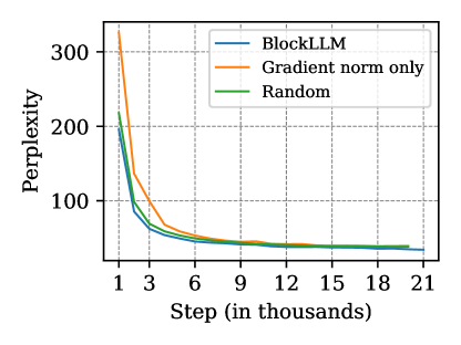
Figure 5: Comparison of random vs greedy BlockLLM on Llama 60m model with 50% parameters chosen.

where $\text{param\_count}(l_{i})$ denotes the number of parameters in layer $l_{i}$. In each iteration $t$, we employ the Adam optimizer to update only the parameters in the layers belonging to the set $D$. We conducted hyper parameter tuning for the patience parameter $m$, which controls the frequency of updates. For a sparsity level of $s=0.5$, we determined the optimal value of $m=75$. To evaluate the effectiveness of the random parameter selection method, we compared evaluation loss with that of BlockLLM. Given that both methods involve updating a similar number of parameters, we expect their memory usage to be comparable. The comparative results are presented in Figure 5.

Our observations indicate that BlockLLM converges faster than the random parameter selection method. Intuitively, this suggests that parameters with higher gradient norms may facilitate more rapid learning. One possible explanation is that parameters with higher gradient norms contribute to larger updates, thereby playing a more significant role in the training process during each iteration. Consequently, these parameters might accelerate the model’s convergence by making more substantial contributions to the optimization trajectory.

Effect of Layer Visit Frequency $f$.

To assess this, we conducted an experiment where parameters were selected based solely on their gradient norms. Specifically, for each layer $l\in L$, we computed the processed gradients $\tilde{G}_{l}$. We then sorted the layers in descending order based on the their processed gradient norms, $||\tilde{G}_{l}||$. From this ordered list, we selected the top $k$ layers that satisfied the sparsity requirement $s$. The results of this experiment are presented in Figure 7. We observed that when parameters were selected solely based on $||\tilde{G}||$, without considering the parameter visit frequency $f_{l}$ for any layer $l\in L$, the loss converged more slowly and to a higher value compared to BlockLLM.

4 Conclusion & Future work

In this paper, we introduced BlockLLM, a novel method for efficiently training large language models. By dynamically estimating and updating the importance of parameters during training, BlockLLM effectively achieves state-of-the-art performance while significantly reducing the memory footprint. Our method achieves the highest validation accuracy on GLUE finetuning tasks, sometimes even surpassing full finetuning. One key aspect of BlockLLM is that it does not presuppose the importance of layers but continuously evaluates and updates parameter importance throughout training. This adaptive approach allows for more flexible and efficient optimization compared to methods that assume certain parameters are critical from the outset. Additionally, BlockLLM preserves the original architecture without altering the model structure or restricting the parameter search space, making it suitable for various LLMs and tasks.

Broader Impacts

Our work aims to reduce the memory and computational requirements of training LLMs. First, our technology democratizes access to LLM training, making it more feasible for student researchers and institutions with limited computational resources to participate in cutting-edge AI research. Furthermore, the low-memory requirements of our method means that one can train with larger batch sizes and achieve faster convergence. This has a direct effect on the environment.

Future works.

Future work on BlockLLM could explore several promising avenues. Currently, our research has focused on parameter selection based on gradient norms, but BlockLLM can be seen as a framework for parameter-efficient training rather than a single algorithm. This opens the door to investigating alternative criteria for parameter selection, potentially tailored to specific problems or tasks. Moreover, while our ablation studies on BlockLLM’s hyperparameters have provided insights into their impact on training, further research is needed to understand how different layers might be affected by greedy parameter selection strategies. BlockLLM also complements existing memory-optimized training techniques, including those discussed in this paper. Exploring the integration of BlockLLM with methods like quantization or GaLore could further reduce memory consumption.

Appendix A Appendix / supplemental material

A.1 Sparsity Accuracy Tradeoff

We performed magnitude pruning on the IMDb pre-trained model [19] weights at various sparsity levels and fine-tuned these pruned models on the GLUE-CoLA dataset [31]. The results of these experiments, detailing the relationship between sparsity and accuracy, are summarized in Table 5.

Sparsity	Accuracy
$0.0$	$79.57$
$0.5$	$78.52$
$0.6$	$74.2$
$0.7$	$67.68$
$0.8$	$69.12$
$0.9$	$69.12$

Table 5: Performance of pruned models at various sparsity levels on GLUE-CoLA dataset.

The accuracy generally declines with increasing sparsity. At $0.5$ sparsity, the performance remains relatively high at $78.52\%$, close to the non-pruned model’s $79.57\%$. However, accuracy drops more significantly to $67.68\%$ at $0.7$ sparsity. Interestingly, at sparsity levels of $0.8$ and $0.9$, accuracy stabilizes around $69.12\%$.

A.2 Analysis of weight magnitudes

In this experiment, we pretrain DistilBERT on the IMDB dataset [19] and then finetune it on GLUE-CoLA [31] with sparsity $s=0.7$. We then plot the histogram of the weight magnitudes $W^{t}$ where $\delta=|w_{i}^{0}-w_{i}^{t}|>\eta$, with $\eta$ as the threshold. We set $\eta=0.001$ in this case.

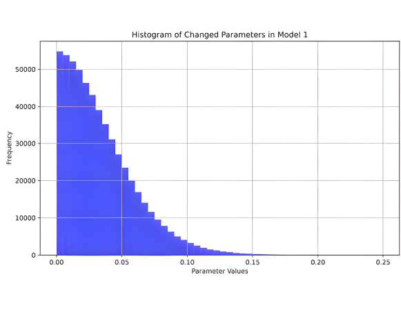
Figure 6: Histogram of changed parameters for $s=0.7$

A.3 Analysis of reduced parameter training

Here, we fine-tuned the GLUE datasets [31] on the DistilBERT model [27] pretrained on the IMDb dataset [19]. We varied the sparsity $s$ and update frequency $m$ while monitoring the number of unique parameters updated $q$. We ran the GLUE-SST2 experiments for $8400$ iterations and GLUE-STSB for $20000$ iterations. Additionally, we tracked the VRAM usage for the GLUE-SST2 dataset to compare it with the memory consumption of full-parameter fine-tuning, which is $7.9$ GB. This comparison aims to determine if reduced parameter training effectively decreases memory usage.

$1-s$	$q$	$m$	Spearman Correlation
$0.01$	$0.05$	$5000$	$88.82$
$0.01$	$0.037$	$10000$	$88.77$

Table 6: Impact of Update Frequency and Sparsity on STSB Dataset

$1-s$	$q$	$m$	Accuracy	VRAM
$0.008$	$0.04$	$2400$	$91.97$	$4.4$
$0.01$	$0.11$	$3000$	$90.94$	$5.5$
$0.02$	$0.13$	$1000$	$90.59$	$5.5$
$0.02$	$0.16$	$2000$	$92.2$	$5.5$

Table 7: VRAM Usage with Different Update Frequencies on SST2 Dataset

Table 6 shows the impact of update frequency $m$ and sparsity $s$ on the STSB dataset, where the correlation remains stable despite changes in update frequency. As $m$ increased too high, the performance declined.

A.4 VRAM memory

All memory values presented in our tables represent actual observed memory usage in gigabytes (GB) rather than estimates. Memory consumption was monitored using the "nvidia-smi" command, and the maximum memory usage recorded during the training process was noted.

A.5 Finetuning on GLUE

In this section, we detail the experimental setup employed for our study. We fine-tuned the pre-trained RoBERTa model [17] , available in the HuggingFace library, on the GLUE benchmark tasks [31]The batch size was set to $32$ for the CoLA dataset, and $16$ for all other datasets. For all tasks, we used $s=0.95$ and $m=\frac{1}{4}\times$ total number of iterations. VRAM memory usage was monitored and recorded as described in Section A.4. The learning rates for the different tasks are as follows.

Table 8: Hyperparameter details for the GLUE experiments

	MRPC	COLA	STS-B	RTE	SST2	MNLI	QNLI	QQP
Learning rate	3E-05	5E-05	3E-05	3E-05	3E-05	3E-05	1E-05	3E-05

A.6 Pre-training on Llama

We present the hyperparameters utilized for training the LLama models with sizes $60$M, $130$M and $350$M in 9. For $60$M and $130$M experiments, the maximum sequence length was set to $256$ with a gradient accumulation of $2$,and for $350$M with a batch size of $128$ with a gradient accumulation of $4$. A cosine annealing schedule was employed for learning rate adjustment, decaying to $10$% of the initial learning rate. For BlockLLM, no learning rate warmup was applied. However, for GaLore, the learning rate was warmed up for the first $10\%$ of training, following the approach outlined in [34]. The parameter $m$ was set to $50$ for all the experiments.

	$60$M	$130$M	$350$M
Learning rate	1E-03	1E-03	1E-03
Total training steps	$10$K	$20$K	$60$K
$s$	$0.5$	$0.5$	$0.5$

Table 9: Hyperparameter Details for Pre-training LLaMA Models with BlockLLM on the C4 Dataset

A.7 Ablation on the hyperparameter $m$

We investigated the sensitivity of the model to the patience parameter $m$ in both fine-tuning and pre-training setups. These experiments were conducted using the GLUE benchmark and the LLaMA 2 model on the C4 dataset. Throughout the experiments, we fixed all parameters of the Adam optimizer and maintained a sparsity level of $s=0.5$ while varying $m$. The results are presented in Figure 7. Our observations indicate that in the fine-tuning setting, the model is relatively insensitive to variations in $m$. Specifically, setting $m=50$ or $m=1000$ did not result in significant performance differences. This finding aligns with the observations reported in [34], which suggest that gradients change more slowly. The gradual nature of gradient changes implies a correspondingly gradual variation in the optimal parameter set, thereby reducing sensitivity to changes in $m$. In contrast, in the pre-training setting, smaller values of $m$ lead to faster convergence. This behavior can be attributed to the presence of noisy gradients in the earlier iterations of pre-training. Consequently, a smaller $m$ helps maintain impactful parameter selection particularly in the initial phase of training, thereby facilitating faster convergence.

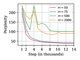
Figure 7: Ablation on the patience parameter $m$. We see that $m$ affects the algorithm and model performance significantly in our pre-training experiments.

References

- Almazrouei et al. [2023] Ebtesam Almazrouei, Hamza Alobeidli, Abdulaziz Alshamsi, Alessandro Cappelli, Ruxandra Cojocaru, Mérouane Debbah, Étienne Goffinet, Daniel Hesslow, Julien Launay, Quentin Malartic, et al. The falcon series of open language models. arXiv preprint arXiv:2311.16867, 2023.
- Belilovsky et al. [2019] Eugene Belilovsky, Michael Eickenberg, and Edouard Oyallon. Greedy layerwise learning can scale to imagenet. In International conference on machine learning, pages 583–593. PMLR, 2019.
- Brown et al. [2020] Tom Brown, Benjamin Mann, Nick Ryder, Melanie Subbiah, Jared D Kaplan, Prafulla Dhariwal, Arvind Neelakantan, Pranav Shyam, Girish Sastry, Amanda Askell, et al. Language models are few-shot learners. Advances in neural information processing systems, 33:1877–1901, 2020.
- Chen et al. [2016] Tianqi Chen, Bing Xu, Chiyuan Zhang, and Carlos Guestrin. Training deep nets with sublinear memory cost. arXiv preprint arXiv:1604.06174, 2016.
- Fan et al. [2019] Angela Fan, Edouard Grave, and Armand Joulin. Reducing transformer depth on demand with structured dropout. arXiv preprint arXiv:1909.11556, 2019.
- Gupta et al. [2022] Manas Gupta, Efe Camci, Vishandi Rudy Keneta, Abhishek Vaidyanathan, Ritwik Kanodia, Chuan-Sheng Foo, Wu Min, and Lin Jie. Is complexity required for neural network pruning? a case study on global magnitude pruning. ArXiv, abs/2209.14624, 2022. URL https://api.semanticscholar.org/CorpusID:252595918.
- Han et al. [2015] Song Han, Huizi Mao, and William J Dally. Deep compression: Compressing deep neural networks with pruning, trained quantization and huffman coding. arXiv preprint arXiv:1510.00149, 2015.
- He et al. [2021] Junxian He, Chunting Zhou, Xuezhe Ma, Taylor Berg-Kirkpatrick, and Graham Neubig. Towards a unified view of parameter-efficient transfer learning. arXiv preprint arXiv:2110.04366, 2021.
- Hu et al. [2021] Edward J Hu, Yelong Shen, Phillip Wallis, Zeyuan Allen-Zhu, Yuanzhi Li, Shean Wang, Lu Wang, and Weizhu Chen. Lora: Low-rank adaptation of large language models. arXiv preprint arXiv:2106.09685, 2021.
- Hu et al. [2023] Zhiqiang Hu, Lei Wang, Yihuai Lan, Wanyu Xu, Ee-Peng Lim, Lidong Bing, Xing Xu, Soujanya Poria, and Roy Ka-Wei Lee. Llm-adapters: An adapter family for parameter-efficient fine-tuning of large language models. arXiv preprint arXiv:2304.01933, 2023.
- Kamalakara et al. [2022] Siddhartha Rao Kamalakara, Acyr Locatelli, Bharat Venkitesh, Jimmy Ba, Yarin Gal, and Aidan N Gomez. Exploring low rank training of deep neural networks. arXiv preprint arXiv:2209.13569, 2022.
- Kaplan et al. [2020] Jared Kaplan, Sam McCandlish, Tom Henighan, Tom B Brown, Benjamin Chess, Rewon Child, Scott Gray, Alec Radford, Jeffrey Wu, and Dario Amodei. Scaling laws for neural language models. arXiv preprint arXiv:2001.08361, 2020.
- Kedia et al. [2021] Akhil Kedia, Sai Chetan Chinthakindi, and Wonho Ryu. Beyond reptile: Meta-learned dot-product maximization between gradients for improved single-task regularization. In Findings of the Association for Computational Linguistics: EMNLP 2021, pages 407–420, 2021.
- Kingma and Ba [2014] Diederik P Kingma and Jimmy Ba. Adam: A method for stochastic optimization. arXiv preprint arXiv:1412.6980, 2014.
- Le Scao et al. [2023] Teven Le Scao, Angela Fan, Christopher Akiki, Ellie Pavlick, Suzana Ilić, Daniel Hesslow, Roman Castagné, Alexandra Sasha Luccioni, François Yvon, Matthias Gallé, et al. Bloom: A 176b-parameter open-access multilingual language model. 2023.
- Lialin et al. [2023] Vladislav Lialin, Sherin Muckatira, Namrata Shivagunde, and Anna Rumshisky. Relora: High-rank training through low-rank updates. In Workshop on Advancing Neural Network Training: Computational Efficiency, Scalability, and Resource Optimization (WANT@ NeurIPS 2023), 2023.
- Liu et al. [2019] Yinhan Liu, Myle Ott, Naman Goyal, Jingfei Du, Mandar Joshi, Danqi Chen, Omer Levy, Mike Lewis, Luke Zettlemoyer, and Veselin Stoyanov. Roberta: A robustly optimized bert pretraining approach. arXiv preprint arXiv:1907.11692, 2019.
- Ma et al. [2023] Xinyin Ma, Gongfan Fang, and Xinchao Wang. Llm-pruner: On the structural pruning of large language models. Advances in neural information processing systems, 36:21702–21720, 2023.
- Maas et al. [2011] Andrew L. Maas, Raymond E. Daly, Peter T. Pham, Dan Huang, Andrew Y. Ng, and Christopher Potts. Learning word vectors for sentiment analysis. In Proceedings of the 49th Annual Meeting of the Association for Computational Linguistics: Human Language Technologies, pages 142–150, Portland, Oregon, USA, June 2011. Association for Computational Linguistics. URL http://www.aclweb.org/anthology/P11-1015.
- Michel et al. [2019] Paul Michel, Omer Levy, and Graham Neubig. Are sixteen heads really better than one? Advances in neural information processing systems, 32, 2019.
- Nutini et al. [2022] Julie Nutini, Issam Laradji, and Mark Schmidt. Let’s make block coordinate descent converge faster: faster greedy rules, message-passing, active-set complexity, and superlinear convergence. Journal of Machine Learning Research, 23(131):1–74, 2022.
- OpenAI [2023] R OpenAI. Gpt-4 technical report. arxiv 2303.08774. View in Article, 2(5), 2023.
- Raffel et al. [2020] Colin Raffel, Noam Shazeer, Adam Roberts, Katherine Lee, Sharan Narang, Michael Matena, Yanqi Zhou, Wei Li, and Peter J Liu. Exploring the limits of transfer learning with a unified text-to-text transformer. Journal of machine learning research, 21(140):1–67, 2020.
- Ramesh et al. [2023] Amrutha Varshini Ramesh, Aaron Mishkin, Mark Schmidt, Yihan Zhou, Jonathan Wilder Lavington, and Jennifer She. Analyzing and improving greedy 2-coordinate updates for equality-constrained optimization via steepest descent in the 1-norm. arXiv preprint arXiv:2307.01169, 2023.
- Rhu et al. [2016] Minsoo Rhu, Natalia Gimelshein, Jason Clemons, Arslan Zulfiqar, and Stephen W Keckler. vdnn: Virtualized deep neural networks for scalable, memory-efficient neural network design. In 2016 49th Annual IEEE/ACM International Symposium on Microarchitecture (MICRO), pages 1–13. IEEE, 2016.
- Sajjad et al. [2023] Hassan Sajjad, Fahim Dalvi, Nadir Durrani, and Preslav Nakov. On the effect of dropping layers of pre-trained transformer models. Computer Speech & Language, 77:101429, 2023.
- Sanh et al. [2019] Victor Sanh, Lysandre Debut, Julien Chaumond, and Thomas Wolf. Distilbert, a distilled version of bert: smaller, faster, cheaper and lighter. arXiv preprint arXiv:1910.01108, 2019.
- Sun et al. [2023] Mingjie Sun, Zhuang Liu, Anna Bair, and J Zico Kolter. A simple and effective pruning approach for large language models. arXiv preprint arXiv:2306.11695, 2023.
- Takase and Kiyono [2021] Sho Takase and Shun Kiyono. Lessons on parameter sharing across layers in transformers. arXiv preprint arXiv:2104.06022, 2021.
- Touvron et al. [2023] Hugo Touvron, Thibaut Lavril, Gautier Izacard, Xavier Martinet, Marie-Anne Lachaux, Timothée Lacroix, Baptiste Rozière, Naman Goyal, Eric Hambro, Faisal Azhar, et al. Llama: Open and efficient foundation language models. arXiv preprint arXiv:2302.13971, 2023.
- Wang et al. [2018] Alex Wang, Amanpreet Singh, Julian Michael, Felix Hill, Omer Levy, and Samuel R Bowman. Glue: A multi-task benchmark and analysis platform for natural language understanding. arXiv preprint arXiv:1804.07461, 2018.
- Wang et al. [2019] Ziheng Wang, Jeremy Wohlwend, and Tao Lei. Structured pruning of large language models. arXiv preprint arXiv:1910.04732, 2019.
- Zeng et al. [2019] Jinshan Zeng, Tim Tsz-Kit Lau, Shaobo Lin, and Yuan Yao. Global convergence of block coordinate descent in deep learning. In International conference on machine learning, pages 7313–7323. PMLR, 2019.
- Zhao et al. [2024] Jiawei Zhao, Zhenyu Zhang, Beidi Chen, Zhangyang Wang, Anima Anandkumar, and Yuandong Tian. Galore: Memory-efficient llm training by gradient low-rank projection. arXiv preprint arXiv:2403.03507, 2024.
- Zhao et al. [2023] Wayne Xin Zhao, Kun Zhou, Junyi Li, Tianyi Tang, Xiaolei Wang, Yupeng Hou, Yingqian Min, Beichen Zhang, Junjie Zhang, Zican Dong, et al. A survey of large language models. arXiv preprint arXiv:2303.18223, 2023.