Efficient, Multimodal, and Derivative-Free Bayesian Inference With Fisher-Rao Gradient Flows

Abstract

In this paper, we study efficient approximate sampling for probability distributions known up to normalization constants. We specifically focus on a problem class arising in Bayesian inference for large-scale inverse problems in science and engineering applications. The computational challenges we address with the proposed methodology are: (i) the need for repeated evaluations of expensive forward models; (ii) the potential existence of multiple modes; and (iii) the fact that gradient of, or adjoint solver for, the forward model might not be feasible.

While existing Bayesian inference methods meet some of these challenges individually, we propose a framework that tackles all three systematically. Our approach builds upon the Fisher-Rao gradient flow in probability space, yielding a dynamical system for probability densities that converges towards the target distribution at a uniform exponential rate. This rapid convergence is advantageous for the computational burden outlined in (i). We apply Gaussian mixture approximations with operator splitting techniques to simulate the flow numerically; the resulting approximation can capture multiple modes thus addressing (ii). Furthermore, we employ the Kalman methodology to facilitate a derivative-free update of these Gaussian components and their respective weights, addressing the issue in (iii).

The proposed methodology results in an efficient derivative-free sampler flexible enough to handle multi-modal distributions: Gaussian Mixture Kalman Inversion (GMKI). The effectiveness of GMKI is demonstrated both theoretically and numerically in several experiments with multimodal target distributions, including proof-of-concept and two-dimensional examples, as well as a large-scale application: recovering the Navier-Stokes initial condition from solution data at positive times.

Keywords: Bayesian Inverse Problems, Sampling, Derivative-Free Methods, Multimodal, Kalman Methodology, Fisher-Rao Gradient Flow, Gaussian Mixtures.

1 Introduction

In this paper we introduce the sampler Gaussian Mixture Kalman Inversion (GMKI) designed for solution of PDE inverse problems for which forward model evaluation is expensive, derivative/adjoint calculations cannot be used and multiple modes are present. In subsection 1.1 we give the context, followed in subsection 1.2 with details of our guiding motivations. Subsection 1.3 describes the key ingredients of the algorithm and subsection 1.4 the contributions. In subsection 1.5 we give a detailed literature review and in subsection 1.6 we describe the organization of the paper.

1.1 Context

Sampling a target probability distribution known up to normalization constants is a classical problem in science and engineering. In this paper, we focus specifically on targets resulting from Bayesian inverse problems [1, 2] involving recovery of unknown parameter $\theta\in\mathbb{R}^{N_{\theta}}$ from noisy observation $y\in\mathbb{R}^{N_{y}}$, through forward model

$$y=\mathcal{G}(\theta)+\eta.$$ (1)

Here, $\mathcal{G}$ denotes the forward mapping which, for the problems we focus on, is nonlinear and requires solution of a partial differential equation (PDE) to evaluate. The observational noise $\eta$ is here assumed to be Gaussian: $\eta\sim\mathcal{N}(0,\Sigma_{\eta})$. By assigning a Gaussian prior $\mathcal{N}(r_{0},\Sigma_{0})$ to the unknown $\theta$, the Bayesian framework leads to the posterior distribution

$$\rho_{\rm post}(\theta) \propto\exp(-\Phi_{R}(\theta)),$$ (2a)

$$\Phi_{R}(\theta) =\Phi(\theta)+\frac{1}{2}\lVert\Sigma_{0}^{-\frac{1}{2}}(\theta-r_{0})\rVert^{2},$$ (2b)

$$\Phi(\theta) =\frac{1}{2}\lVert\Sigma_{\eta}^{-\frac{1}{2}}(y-\mathcal{G}(\theta))\rVert^{2}.$$ (2c)

Here $\Phi$ is the negative log likelihood. Minimization of $\Phi_{R}$ is a nonlinear least-squares problem which defines the maximum a posterior (MAP) point estimator for the Bayesian inverse problem. It is the goal of this paper to develop efficient samplers for $\rho_{\rm post}$ defined by $\Phi_{R}$ in the specific setting which we now outline.

1.2 Guiding Motivations

We give more detail concerning the motivations behind the specific sampler developed here. Firstly we note that an appropriate unit of cost in solution of Bayesian inverse problems is the evaluation of $\mathcal{G}$ as this will be required multiple times for methods such as MCMC [3] and SMC [4, 5]; when evaluation of $\mathcal{G}$ requires running large scale PDE solvers fast convergence is paramount. Secondly we note that multiple modes, caused by multiple minimizers of $\Phi_{R}$, cause many samplers to become slow [6], expending multiple steps in one mode before moving to another [7, 8]; in addition, many Gaussian approximation based methods are unable to capture multiple modes. Nevertheless, exploring all these modes is necessary since missing one could lead to detrimental effects on engineering or science predictions; Thirdly we note that the gradient of $\Phi_{R}$ may not be available or even feasible. This might be because the computational models are only given as a black box (e.g. in global climate model calibration [9, 10]), the numerical methods are not differentiable (e.g. in the embedded boundary method [11, 12, 13, 14] and adaptive mesh refinement [15, 16]), or because of inherently discontinuous physics (i.e., in fracture [17] or cloud modeling [18, 19]). In this paper we address these three challenges by combining, respectively, Fisher-Rao gradient flows, Gaussian mixture approximations, and Kalman methodology. The resulting sampler, Gaussian Mixture Kalman Inversion (GMKI), is fast due to the uniform exponential convergence of Fisher-Rao gradient flows, can capture multiple modes since Gaussian mixture approximations are employed, and is derivative-free thanks to the systematic Kalman methodology.

1.3 Key Ingredients of GMKI

In sampling, it is widely accepted practice to construct a dynamical system for a density that gradually evolves to the posterior distribution, or its approximation, after a specified finite time or at infinite time. Numerical approximation of this dynamics, using either particle or parametric methods, leads to practical algorithms. These include sequential Monte Carlo (SMC, specified finite time) [4] and Markov chain Monte Carlo (MCMC, infinite time) [3] that are commonly used in Bayesian inference. In recent years, gradient flows in the probability space have become a popular choice of dynamical systems [20, 21, 22]; their study presents the opportunity to profoundly influence our understanding and development of sampling algorithms.

In general, the convergence rates of different gradient flows can vary significantly. In this paper, we focus on the Fisher-Rao gradient flow of the Kullback–Leibler (KL) divergence [23, 24, 25]:

$$\frac{\partial\rho_{t}}{\partial t}=\rho_{t}\bigl{(}\log\rho_{\rm post}-\log\rho_{t}\bigr{)}-\rho_{t}\mathbb{E}_{\rho_{t}}[\log\rho_{\rm post}-\log\rho_{t}].$$ (3)

The Fisher-Rao gradient flow converges to its steady state, $\rho_{\rm post}$, exponentially fast, with a rate of $\mathcal{O}(e^{-t})$; see [25, Proposition 3.23] and also [23, 24, 26]. This convergence rate is uniform and independent of $\rho_{\rm post}$, in particular its log-Sobolev constant, which typically determines the convergence rates of other gradient flows, such as the Wasserstein gradient flow. It is worth noting that the log-Sobolev constant may behave poorly when the posterior distribution $\rho_{\rm post}$ is highly anisotropic or multimodal [7, 8]. Thus, we consider Eq. 3 as a desirable flow for sampling general distributions.

We introduce numerical approximations of Eq. 3 to construct practical algorithms. Particle methods represent the current density $\rho_{t}$ by a (possibly weighted) sum of Dirac measures evaluated at an ensemble of particles. The flow Eq. 3 can then be realized as a birth-death dynamics of these particles [23, 24]. However, the birth-death rate depends on the density, so it is necessary to constantly reconstruct $\rho_{t}$ from the empirical particle distribution. In [23, 24], kernel density estimators have been applied for the reconstruction, but their performance may be affected when the dimension of the problem becomes large. Moreover, birth-death dynamics alone cannot change the support of the distribution, so additional steps need to be added to explore the space [23, 24, 27]; such exploration steps change the dynamics and may also lead to challenges in high dimensional problems.

Parametric methods, which reduce the gradient flow into some parametric density space, constitute another common choice of numerical approximation. One way to do this is to project the flow Eq. 3 into the Gaussian space [25, 28, 29], via a moment closure approach. The resulting system for the mean and covariance is given by [22]:

$$\frac{\mathrm{d}m_{t}}{\mathrm{d}t}=C_{t}\mathbb{E}_{\rho_{a_{t}}}[\nabla_{\theta}\log\rho_{\rm post}]\qquad\frac{\mathrm{d}C_{t}}{\mathrm{d}t}=C_{t}+C_{t}\mathbb{E}_{\rho_{a_{t}}}[\nabla_{\theta}\nabla_{\theta}\log\rho_{\rm post}]C_{t},$$ (4)

where $\rho_{t}$ in Eq. 3 is approximated by a Gaussian $\rho_{a_{t}}=\mathcal{N}(m_{t},C_{t})$ in Eq. 4; here $a_{t}=(m_{t},C_{t})$ is the unknown parameter. We note that one may also derive the above flow by natural gradient methods in variational inference [30, 31, 32]; see discussions in [25]. Theoretically, it has been shown in [25] that Eq. 4 converges exponentially fast to the best Gaussian approximation of $\rho_{\rm post}$ in the KL divergence sense, when $\rho_{\rm post}$ is log-concave. Therefore, by simulating Eq. 4, we get a Gaussian approximation of the posterior; this can be done through a direct time integration or ensemble methods.

More generally, for multimodal problems, Gaussian mixture approximations have been studied in the literature under the variational inference framework [33]. These approaches require the evaluation of the gradient and sometimes even the Hessian matrix of $\log\rho_{\rm post}$, as shown in Eq. 4, which are not directly feasible for the type of problems which are our focus in this paper.

On the other hand, Kalman methodology has emerged as an effective methodology for sampling for both filter and inverse problems [34, 35, 36, 37, 38, 39, 40]. Similar to the parametric methods discussed above, it relies on Gaussian approximations; however, it additionally utilizes the structure of the problem, i.e., the least-squares form of the posterior as described in Eq. 2. Notably, the Kalman methodology can lead to derivative-free algorithms such as the Ensemble Kalman Filter (EnKF), Unscented Kalman Filter (UKF), and Ensemble Kalman Inversion (EKI), all defined in [40]. Moreover, the recent work on EKI and its variants in [41] can be interpreted as applying Kalman-type approximations to the Fisher-Rao gradient flow Eq. 3, although this gradient structure was not explicitly pointed out in the original paper. The effectiveness of this method has been demonstrated on large-scale inverse problems in science and engineering, with up to hundreds of dimensions. However, since only Gaussian approximations are used, the method may not be suitable for multimodal posterior distributions.

1.4 Contributions

The primary focus of this paper is to extend the Kalman methodology in [41] to Gaussian mixture approximations of the Fisher-Rao gradient flow. This leads to GMKI, a derivative-free sampler that converges fast and captures multiple modes for the challenging inversion problems studied here. We make the following contributions:

1. We propose an operator splitting approach to integrate the Fisher-Rao gradient flow in time, which leads to an exploration step that explores the space freely and an exploitation step that harnesses the data and prior information. We prove the resulting exploration-exploitation scheme converges exponentially fast to the target distribution at the discrete time level (Section 2).

2. We demonstrate a connection between the continuous time limit of the pre-existing algorithm in [41] and Gaussian variational inference (Section 3).

3. We apply Gaussian mixture approximations to the exploration-exploitation scheme. We utilize the Kalman methodology to update the weights and locations of the mixtures. This leads to our derivative-free algorithm, GMKI, for sampling multimodal distributions (Section 4).

4. We analyze GMKI by deriving the continuous time limit of the dynamics. Based on the continuous dynamics, we study its exploration effects, establish its affine invariant property, connect the methodology to variational inference with Gaussian mixtures, and investigate the convergence properties (Section 5).

5. We demonstrate, on one/two-dimensional model problems as well as a high-dimensional application (recovering the Navier-Stokes initial condition from solution data at positive times), that GMKI is able to capture multiple modes. The estimated posterior distributions by GMKI match well with those obtained by MCMC (when it is feasible). The latter typically needs $\mathcal{O}(10^{4})$ forward evaluations or more, whilst for GMKI only $\mathcal{O}(10)$ iterations suffice, leading to tremendous speed-ups; our code is accessible online(Section 6).

1.5 Literature Review

The review of relevant literature concerns SMC and MCMC, variational inference, gradient flows and Kalman methodology.

1.5.1 SMC and MCMC

Sequential Monte Carlo (SMC) [42] and Markov chain Monte Carlo (MCMC) [3] are common approaches used in Bayesian inference for sampling posteriors. They lead to dynamical systems of densities that progressively converge to the target distribution. For SMC, the dynamical system operates over finite time intervals so converges fast in the density level, but numerical approximations of the dynamical system can be challenging, with difficulties such as weight collapses. Such issues are more pronounced in the case of multimodal posteriors, requiring a substantial number of particles and a good initialization for SMC to succeed, due to its lack of exploration. The Fisher-Rao gradient flow used in this paper can be seen as an infinite time extension of SMC that allows efficient exploration while converging exponentially fast in the density level. MCMC approaches typically require $O(10^{4})$ model runs, or more, for the type of PDE-based inversion arising in this paper; thus they are too costly. Moreover, most MCMC approaches are based on local moves and face significant challenges in the multimodal scenario.

1.5.2 Variational Inference

Variational inference [43, 44, 45] addresses the sampling problem Eq. 2 using optimization, typically with a lower computational cost compared to MCMC. The objective function, often chosen to be the KL divergence between the target distribution and a variational distribution, is minimized to get a closest approximate distribution within the variational distribution family. Gaussian distributions and Gaussian mixtures are often used as the variational distribution [46, 47, 33, 48]. The concept of natural gradients [30, 28, 33, 31, 32] has been widely used to derive efficient optimization algorithms for variational inference. These algorithms typically require evaluations of gradient information for the log density. We also note that the Gaussian and Gaussian mixture ansatz has been used in conjunction with the Dirac-Frenkel variational principle to solve time-dependent PDEs of wave functions and probability densities [49, 50]. When the PDE is the Fisher-Rao gradient flow, these methods can recover the parameter dynamics obtained by natural gradient flow in variational inference [51].

1.5.3 Fisher-Rao Gradient Flow

The Fisher-Rao gradient flow plays a key role in the design of sampling algorithms studied in this paper. There is a vast literature on the use of gradient flows of the KL divergence in the density space, employing different metric tensors, for sampling. We specifically focus on the Fisher-Rao metric, introduced by C.R. Rao [52], to derive the gradient flow Eq. 3, as it is the only metric, up to scaling, invariant under any diffeomorphism of the parameter space [53, 54, 55]. This invariance leads to a gradient flow converging at rate independent of the target distribution. In practice, the Fisher-Rao gradient flow and its simulation by birth-death processes have been used in sequential Monte Carlo samplers to reduce the variance of particle weights [4] and accelerate Langevin sampling [23, 24, 27] and statistical learning [56]. Kernel approximation of the flow has also been considered [57, 58]. Gaussian approximation of the Fisher-Rao gradient flow is studied in [25], with close connections to natural gradient methods in variational inference.

1.5.4 Kalman Methodology

The Kalman methodology encompasses a general class of approaches for solving filtering and inverse problems. They are based on replacing the Bayesian inference step in a filter, which may be viewed as governed by a prior to posterior map, by an approximate transport map which is exact for Gaussians; inverse problems are solved by linking them to a filter. Ensemble Kalman methods give rise to derivative-free algorithms, and are appropriate for solving filtering and inverse problems in which the desired probability distribution is close to Gaussian [34, 59, 60, 61, 41].

Beyond Gaussian approximations, a strand of research has extended Kalman filters to operate on Gaussian mixtures [62, 63, 64, 65, 66, 67, 68, 69]. These methods model both prior and posterior distributions using Gaussian mixture distributions, leveraging a componentwise application of the Kalman methodology for each Gaussian component. Various techniques, such as recluster analysis and resampling techniques [70, 71, 72, 73, 74], as well as localization techniques [75, 76, 77], have been developed to enhance the robustness of these approaches. Nevertheless, existing methods in this category are tailored to transform a Gaussian mixture prior into a Gaussian mixture posterior; they can be understood as a Gaussian mixture approximation of the dynamics in SMC. The resulting methods lack full exploration of the space of possible solutions. In contrast, the GMKI method introduced in this paper is designed for sampling general multimodal posterior distributions without specifying multimodal structures on the prior. Unlike previous approaches, GMKI incorporates gradient flows, resulting in theoretical advantages manifest in its analysis. In practice, GMKI’s exploration component enables effective traversal of the solution space, leading to robust performance without weight collapse.

1.6 Organization

The paper is organized as follows. In Section 2, we introduce the Fisher-Rao gradient flow and the exploration-exploitation scheme for discretizing the flow in time. In Section 3, the Gaussian approximation approach for spatial approximation is reviewed. In Section 4, the proposed GMKI approach is presented, which relies on the Gaussian mixture approximation and Kalman methodology. In Section 5, the continuous time dynamics of the GMKI approach is derived and analyzed. In Section 6, numerical experiments are provided. We make concluding remarks in Section 7.

2 Fisher-Rao Gradient Flow

In the following two subsections, we (i) briefly describe the Fisher-Rao gradient flow in the time-continuous settings; and (ii) introduce our operator splitting approach for simulating this flow in practice.

2.1 Continuous Flow

In this paper we focus on the gradient flow arising from using KL divergence as the energy and Fisher-Rao as the metric; the resulting flow has the form

$$\frac{\partial\rho_{t}}{\partial t}=\rho_{t}\bigl{(}\log\rho_{\rm post}-\log\rho_{t}\bigr{)}-\rho_{t}\mathbb{E}_{\rho_{t}}[\log\rho_{\rm post}-\log\rho_{t}].$$ (5)

We have the following uniform exponential convergence result for this flow ([25, Prop. 3.23]; see also related results in [23, 24, 26, 78]):

Proposition 1.

Let $\rho_{t}$ satisfy Eq. 5. Assume there exist constants $K,B>0$ such that the initial density $\rho_{0}$ satisfies

$$e^{-K(1+|\theta|^{2})}\leq\frac{\rho_{0}(\theta)}{\rho_{\rm post}(\theta)}\leq e^{K(1+|\theta|^{2})},$$ (6)

and $\rho_{0},\rho_{\rm post}$ have bounded second moments

$$\int|\theta|^{2}\rho_{0}(\theta)\mathrm{d}\theta\leq B,\quad\int|\theta|^{2}\rho_{\rm post}(\theta)\mathrm{d}\theta\leq B.$$ (7)

Then, for any $t\geq\log\bigl{(}(1+B)K\bigr{)}$,

$${\rm KL}[\rho_{t}\|\rho_{\rm post}]\leq(2+B+eB)Ke^{-t}.$$ (8)

Accurate numerical simulation of Eq. 5 thus has the potential to exhibit uniform exponential convergence across a wide range of targets $\rho_{\rm post}$.

2.2 Time-Stepping via Operator Splitting

As a first step towards derivation of an algorithm we apply operator splitting to Eq. 5. Abusing notation we let $\rho_{n}$ denote our approximation of $\rho_{t_{n}}$ at time $t=t_{n}=n\Delta t$ and solve sequentially

$$\frac{\partial\hat{\rho}_{t}}{\partial t}=-\hat{\rho}_{t}(\log\hat{\rho}_{t}-\mathbb{E}_{\hat{\rho}_{t}}[\log\hat{\rho}_{t}]),\quad\hat{\rho}_{t_{n}}=\rho_{n},\quad t_{n}\leq t\leq t_{n+1},$$ (9)

and

$$\frac{\partial\check{\rho}_{t}}{\partial t}=\check{\rho}_{t}(\log\rho_{\rm post}-\mathbb{E}_{\check{\rho}_{t}}[\log\rho_{\rm post}]),\quad\check{\rho}_{t_{n}}=\hat{\rho}_{t_{n+1}},\quad t_{n}\leq t\leq t_{n+1}.$$ (10)

The map $\rho_{n}\mapsto\rho_{n+1}$ is then defined by setting $\rho_{n+1}=\check{\rho}_{t_{n+1}}$. Further abusing notation we write $\hat{\rho}_{t_{n+1}}=\hat{\rho}_{n+1}$ and $\check{\rho}_{t_{n+1}}=\check{\rho}_{n+1}.$ Note that all of $\rho_{n},\hat{\rho}_{n+1}$ and $\check{\rho}_{n+1}$ are functions of $\theta$. Both Eq. 9 and Eq. 10 admit explicit solutions and we may write

$$\hat{\rho}_{n+1}(\theta)\propto\rho_{n}(\theta)^{e^{-\Delta t}},$$ (11a)

$$\check{\rho}_{n+1}(\theta)\propto\hat{\rho}_{n+1}(\theta)\rho_{\rm post}(\theta)^{\Delta t}.$$ (11b)

Furthermore, using the first order approximation $e^{-\Delta t}\approx 1-\Delta t$ and the explicit formula (2) for $\rho_{\rm post},$ we obtain the following time-stepping scheme:

$$\hat{\rho}_{n+1}(\theta)\propto\rho_{n}(\theta)^{1-\Delta t},$$ (12a)

$$\rho_{n+1}(\theta)\propto\hat{\rho}_{n+1}(\theta)\rho_{\rm post}(\theta)^{\Delta t}\propto\hat{\rho}_{n+1}(\theta)e^{-\Delta t\Phi_{R}(\theta)}.$$ (12b)

Let us make some observations of the scheme Eq. 12. The step Eq. 12a tends to expand the distribution to explore the state space, while Eq. 12b multiplies the current distribution by the “posterior function” to exploit the data and prior information. It is worth noting that the exploration-exploitation concept distinguishes the present approach from sequential Monte Carlo [4] and other homotopy based approaches for sampling [79], which instead rely on the updating rule

$$\rho_{n+1}(\theta)\propto\rho_{n}(\theta)e^{-\Delta t\Phi(\theta)}$$

to deform the prior into the posterior in one unit time. The iteration Eq. 12 is first proposed as the basis for sampling algorithms in [41] as a methodology to remedy the ensemble collapse of EKI in long time asymptotics; however, the connection to gradient flows is not pointed out. We note that the iteration Eq. 12 also connect to the tempering (or annealing) approaches that are commonly used in the Monte Carlo literature [80, 81, 82]. Finally Eq. 12 can also be interpreted as an entropic mirror descent algorithm in optimization [83].

The exploration-exploitation time-stepping scheme Eq. 12 inherits the convergence property of the continuous flow; see Proposition 2. The proof can be found in A.

Proposition 2.

Under the assumptions in Proposition 1, let $\rho_{n}$ solve Eq. 12, then for any $n\geq|\frac{\log((1+B)K)}{\log(1-\Delta t)}|$, it holds that

$$\mathrm{KL}\left[\rho_{n}\|\rho_{\rm post}\right]\leq(2+B+eB)K(1-\Delta t)^{n}.$$ (13)

Proposition 2 shows that $\rho_{\rm post}$ is the fixed point of the time-stepping scheme Eq. 12.

3 Gaussian Approximation and Kalman Methodology

In this section, we discuss the Gaussian approximation of the scheme Eq. 12 through the Kalman methodology. In doing so we review the necessary techniques and pave the way for constructing our Gaussian mixture approximations in the next section.

In [41], the authors used Gaussian distributions to approximate the evolution of densities defined by Eq. 12. More precisely, assume $\rho_{n}=\mathcal{N}(m_{n},C_{n})$. Then, the first exploration step Eq. 12a leads to

$$\hat{\rho}_{n+1}=\mathcal{N}(\widehat{m}_{n+1},\widehat{C}_{n+1})=\mathcal{N}(m_{n},\frac{1}{1-\Delta t}C_{n}).$$ (14)

The distribution still remains Gaussian. However, the second exploitation step Eq. 12b will map out of the space of Gaussian densities, unless $\Phi_{R}$ is quadratic. In [41], the Kalman methodology is employed to approximate Eq. 12b, which is similar to the analysis step in the Kalman filter. More precisely, the methodology starts with the following artificial inverse problem:

$$x=\mathcal{F}(\theta)+\nu,$$ (15)

where we have

$$x=\begin{bmatrix}y\\ r_{0}\end{bmatrix}\quad\mathcal{F}(\theta)=\begin{bmatrix}\mathcal{G}(\theta)\\ \theta\end{bmatrix}\quad\Sigma_{\nu}=\begin{bmatrix}\Sigma_{\eta}&0\\ 0&\Sigma_{0}\end{bmatrix}.$$ (16)

Here, we set the prior on $\theta$, denoted by $\rho(\theta)$, to be $\hat{\rho}_{n+1}(\theta)$, and the observation noise $\nu\sim\mathcal{N}(0,\frac{\Sigma_{\nu}}{\Delta t})$. Following Bayes rule, the posterior distribution of the artificial inverse problem is

$$\rho(\theta|x)=\frac{\rho(\theta)\rho(x|\theta)}{\rho(x)}\propto\rho(\theta)e^{-\Delta t\Phi_{R}(\theta)}=\rho_{n+1}(\theta),$$ (17)

which matches the output of the step Eq. 12b. Here we used the fact that Eq. 2 can be rewritten as

$$\Phi_{R}(\theta)=\frac{1}{2}\lVert\Sigma_{\nu}^{-\frac{1}{2}}(x-\mathcal{F}(\theta))\rVert^{2}.$$ (18)

The Kalman methodology for approximating the posterior $\rho(\theta|x)$ may now be adopted. One first forms a Gaussian approximation of the joint distribution of $\theta$ and $\mathcal{F}(\theta)+\nu$, via standard moment matching, yielding

$$\rho^{\rm G}(\theta,\mathcal{F}(\theta)+\nu)\sim\mathcal{N}\Big{(}\begin{bmatrix}\theta\\ x\end{bmatrix};\begin{bmatrix}\widehat{m}_{n+1}\\ \widehat{x}_{n+1}\end{bmatrix},\begin{bmatrix}\widehat{C}_{n+1}&\widehat{C}^{\theta x}_{n+1}\\ \widehat{C}_{n+1}^{{\theta x}^{T}}&\widehat{C}^{xx}_{n+1}\end{bmatrix}\Big{)},$$ (19)

where $\widehat{m}_{n+1},\widehat{C}_{n+1}$ are as specified previously, and

$$\begin{split}\widehat{x}_{n+1}=\mathbb{E}[\mathcal{F}(\theta)],\quad\widehat{C}^{\theta x}_{n+1}=\mathrm{Cov}[\theta,\mathcal{F}(\theta)],\quad\widehat{C}^{xx}_{n+1}=\mathrm{Cov}[\mathcal{F}(\theta)+\nu]=\mathrm{Cov}[\mathcal{F}(\theta)]+\frac{\Sigma_{\nu}}{\Delta t}.\end{split}$$ (20)

In the above, the expectation and covariance is taken over $\theta\sim\hat{\rho}_{n+1}$. These integrals can be computed using Monte Carlo methods or quadrature rules.

Then, one can condition the joint Gaussian distribution Eq. 19 on the event $\mathcal{F}(\theta)+\nu=x$, to get a Gaussian approximation of the posterior $\rho(\theta|x)$. In detail, using the Gaussian conditioning formula, one obtains

$$\rho_{n+1}(\theta)\approx\rho^{\rm G}(\theta|\mathcal{F}(\theta)+\nu=x)=\mathcal{N}(\theta;m_{n+1},C_{n+1}),$$ (21a)

where

$$m_{n+1} =\widehat{m}_{n+1}+\widehat{C}^{\theta x}_{n+1}(\widehat{C}^{xx}_{n+1})^{-1}(x-\widehat{x}_{n+1}),$$ (22a)

$$C_{n+1} =\widehat{C}_{n+1}-\widehat{C}^{\theta x}_{n+1}(\widehat{C}^{xx}_{n+1})^{-1}(\widehat{C}_{n+1}^{{\theta x}})^{T}.$$ (22b)

Combining the two updates Eq. 14 and Eq. 22 leads to a Gaussian approximation scheme for solving the discrete Fisher-Rao gradient flow Eq. 12. The scheme is based on the Kalman methodology and is derivative free. Some theoretical and numerical studies of this scheme can be found in [41].

Remark 1.

We can connect the Gaussian approximation based on the Kalman methodology and the approximation Eq. 4 obtained by Gaussian variational inference. To do so we consider the continuous time limit of Eq. 22, calculated in [41, Eq. A.2], as

$$\frac{\mathrm{d}m_{t}}{\mathrm{d}t} =\widehat{C}_{t}^{\theta x}\Sigma_{\nu}^{-1}(x-\widehat{x}_{t}),\qquad\frac{\mathrm{d}C_{t}}{\mathrm{d}t} =C_{t}-\widehat{C}_{t}^{\theta x}\Sigma_{\nu}^{-1}({\widehat{C}_{t}^{\theta x}})^{T},$$ (23)

where $\widehat{x}_{t}=\mathbb{E}_{\rho_{t}}[\mathcal{F}(\theta)]$, $\widehat{C}_{t}^{\theta x}=\mathbb{E}_{\rho_{t}}\bigl{[}\bigl{(}\theta-m\bigr{)}\otimes\bigl{(}\mathcal{F}(\theta)-\mathbb{E}\mathcal{F}(\theta)\bigr{)}\bigr{]}$ and the expectation is taken with respect to the distribution $\rho_{t}(\theta)=\mathcal{N}(\theta;m_{t},C_{t})$. We can view Eq. 23 as a derivative-free approximation of Eq. 4 through the statistical linearization [40, Sec 4.3.2] approach. More precisely, by Stein’s identity which utilizes the integration by parts formula for Gaussian measures, we have the relation $\mathbb{E}_{\rho_{t}}[\nabla_{\theta}\mathcal{F}(\theta)]=C_{t}^{-1}\widehat{C}^{\theta x}_{t}$. Statistical linearization makes the approximation $\nabla_{\theta}\mathcal{F}(\theta)\approx C_{t}^{-1}\widehat{C}^{\theta x}_{t}$ for all $\theta$; the approximation is exact when $\mathcal{F}$ is linear. Based on it, we can approximate the right hand side in the equation of the mean in Eq. 4 as follows:

$$C_{t}\mathbb{E}_{\rho_{t}}[\nabla_{\theta}\log\rho_{\rm post}]=C_{t}\mathbb{E}_{\rho_{t}}[\nabla_{\theta}\mathcal{F}(\theta)\Sigma_{\nu}^{-1}(x-\mathcal{F}(\theta))]\approx\widehat{C}_{t}^{\theta x}\Sigma_{\nu}^{-1}(x-\widehat{x}_{t}),$$ (24)

where in the first identity we used the fact $\rho_{\rm post}\propto\exp(-\frac{1}{2}\|\Sigma_{\nu}^{-1/2}(\mathcal{F}(\theta)-x)\|^{2})$, and we used the statistical linearization approximation in the last derivation.

The stochastic linearization essentially approximates $\nabla_{\theta}\mathcal{F}(\theta)$ by a constant vector (which is why the term linearization is used); under this approximation, the Hessian $\nabla_{\theta}\nabla_{\theta}\mathcal{F}(\theta)$ is zero. Based on this fact, we obtain, for the equation of the covariance in Eq. 4, that

$$C_{t}-C_{t}\mathbb{E}_{\rho_{t}}[\nabla_{\theta}\nabla_{\theta}\log\rho_{\rm post}]C_{t} \approx C_{t}-C_{t}\mathbb{E}_{\rho_{t}}[\nabla_{\theta}\mathcal{F}(\theta)\Sigma_{\nu}^{-1}\nabla_{\theta}\mathcal{F}(\theta)^{T}]C_{t}$$ (25)

$$\approx C_{t}-\widehat{C}^{\theta x}_{t}\Sigma_{\nu}^{-1}({\widehat{C}^{\theta x}}_{t})^{T}.$$

Thus, we recover Eq. 23. In this sense, we can understand the Kalman methodology in the continuous limit as applying a statistical linearization approximation to the dynamics obtained in variational inference.  $\lozenge$

4 Gaussian Mixture Kalman Inversion

In this section we study the use of Gaussian mixture models to approximate the evolution $\rho_{n}\mapsto\rho_{n+1}$ defined by Eq. 12. We assume that at step $n$ the distribution has the form of a $K$-component Gaussian mixture:

$$\rho_{n}(\theta)=\sum_{k=1}^{K}w_{n,k}\mathcal{N}(\theta;m_{n,k},C_{n,k}),$$

where $w_{n,k}\geq 0$, $\sum_{k=1}^{K}w_{n,k}=1$. It remains to specify updates of the weights and Gaussian components, through the map defined by Eq. 12. In the two subsequent subsections we consider steps (12a) and (12b) respectively.

4.1 The Exploration Step

The first step Eq. 12a, $\hat{\rho}_{n+1}(\theta)$ $\propto\rho_{n}(\theta)^{1-\Delta t}$, is not closed in the space of $K$-component Gaussian mixtures. Thus, we choose to approximate $\hat{\rho}_{n+1}$ by a new Gaussian mixture model

$$\hat{\rho}_{n+1}\approx\hat{\rho}^{\rm GM}_{n+1}=\sum_{k=1}^{K}\hat{w}_{n+1,k}\mathcal{N}(\theta;\widehat{m}_{n+1,k},\widehat{C}_{n+1,k}).$$

Note that $\rho_{n}(\theta)^{1-\Delta t}=\rho_{n}(\theta)^{-\Delta t}\rho_{n}(\theta)$. We will determine the parameters of the new Gaussian mixture model by applying Gaussian moment matching to each component $\rho_{n}(\theta)^{-\Delta t}w_{n,k}\mathcal{N}(\theta;m_{n,k},C_{n,k})$ in $\rho_{n}(\theta)^{-\Delta t}\rho_{n}(\theta)$. More specifically, we first rewrite the power of a Gaussian mixture as follows:

$$\hat{\rho}_{n+1}(\theta)\propto \Bigl{(}\sum_{k=1}^{K}w_{n,k}\mathcal{N}(\theta;m_{n,k},C_{n,k})\Bigr{)}^{1-\Delta t}$$

$$= \sum_{k=1}^{K}\Bigl{[}w_{n,k}\mathcal{N}(\theta;m_{n,k},C_{n,k})\Bigl{(}\sum_{i=1}^{K}w_{n,i}\mathcal{N}(\theta;m_{n,i},C_{n,i})\Bigr{)}^{-\Delta t}\Bigr{]}$$

$$= \sum_{k=1}^{K}\Bigl{[}f_{n,k}(\theta)\mathcal{N}(\theta;m_{n,k},\frac{C_{n,k}}{1-\Delta t})\Bigr{]},$$

where

$$f_{n,k}(\theta)=\frac{(2\pi)^{\frac{\Delta tN_{\theta}}{2}}}{(1-\Delta t)^{\frac{N_{\theta}}{2}}}w_{n,k}^{1-\Delta t}{\det(C_{n,k})}^{\frac{\Delta t}{2}}\Bigl{(}\frac{w_{n,k}\mathcal{N}(\theta;m_{n,k},C_{n,k})}{\sum_{i=1}^{K}w_{n,i}\mathcal{N}(\theta;m_{n,i},C_{n,i})}\Bigr{)}^{\Delta t}.$$

We approximate each component above by a Gaussian distribution:

$$f_{n,k}(\theta)\mathcal{N}(\theta;m_{n,k},\frac{C_{n,k}}{1-\Delta t})\approx\hat{w}_{n+1,k}\mathcal{N}(\theta;\widehat{m}_{n+1,k},\widehat{C}_{n+1,k}),$$ (26)

where we set

$$\hat{w}_{n+1,k} =\int f_{n,k}(\theta)\mathcal{N}(\theta;m_{n,k},\frac{C_{n,k}}{1-\Delta t})\mathrm{d}\theta,$$ (27a)

$$\widehat{m}_{n+1,k} =\frac{1}{\hat{w}_{n+1,k}}\int\theta f_{n,k}(\theta)\mathcal{N}(\theta;m_{n,k},\frac{C_{n,k}}{1-\Delta t})\mathrm{d}\theta,$$ (27b)

$$\widehat{C}_{n+1,k} =\frac{1}{\hat{w}_{n+1,k}}\int(\theta-\widehat{m}_{n+1,k})(\theta-\widehat{m}_{n+1,k})^{T}f_{n,k}(\theta)\mathcal{N}(\theta;m_{n,k},\frac{C_{n,k}}{1-\Delta t})\mathrm{d}\theta.$$ (27c)

Here, we determine $\hat{w}_{n+1,k}$, $\widehat{m}_{n+1,k}$, and $\widehat{C}_{n+1,k}$ by moment matching of both sides in Eq. 26. These integrals can be evaluated by Monte Carlo method or quadrature rules. Then, we normalize $\{\hat{w}_{n+1,k}\}_{k=1}^{k=K}$ so that their summation is 1. The updates (27) determine $\hat{\rho}^{\rm GM}_{n+1}$.

4.2 The Exploitation Step

The second step Eq. 12b leads to

$$\rho_{n+1}(\theta) \propto\hat{\rho}^{\rm GM}_{n+1}(\theta)e^{-\Delta t\Phi_{R}(\theta)}$$

$$\propto\sum_{k=1}^{K}\hat{w}_{n+1,k}\mathcal{N}(\theta;\widehat{m}_{n+1,k},\widehat{C}_{n+1,k})e^{-\Delta t\Phi_{R}(\theta)}.$$

Now, the goal is to approximate the above $\rho_{n+1}$ by a $K$-component Gaussian mixture $\sum_{k=1}^{K}w_{n+1,k}\mathcal{N}(\theta;m_{n+1,k},C_{n+1,k})$. We adopt the Kalman methodology described in Section 3, to update each Gaussian component individually such that

$$\hat{w}_{n+1,k}\mathcal{N}(\theta;\widehat{m}_{n+1,k},\widehat{C}_{n+1,k})e^{-\Delta t\Phi_{R}(\theta)}\approx w_{n+1,k}\mathcal{N}(\theta;m_{n+1,k},C_{n+1,k}).$$ (28)

More precisely, following (22), for each $1\leq k\leq K$, we obtain the mean and covariance updates as

$$\begin{split}m_{n+1,k}&=\widehat{m}_{n+1,k}+\widehat{C}_{n+1,k}^{\theta x}(\widehat{C}_{n+1,k}^{xx})^{-1}(x-\widehat{x}_{n+1,k}),\\ C_{n+1,k}&=\widehat{C}_{n+1,k}-\widehat{C}_{n+1,k}^{\theta x}(\widehat{C}_{n+1,k}^{xx})^{-1}(\widehat{C}_{n+1,k}^{\theta x})^{T},\end{split}$$ (29)

where

$$\begin{split}\widehat{x}_{n+1,k}=\mathbb{E}[\mathcal{F}(\theta)]\qquad\widehat{C}_{n+1,k}^{\theta x}=\mathrm{Cov}[\theta,\mathcal{F}(\theta)]\qquad\widehat{C}_{n+1,k}^{xx}=\mathrm{Cov}[\mathcal{F}(\theta)]+\frac{\Sigma_{\nu}}{\Delta t},\end{split}$$

with $\theta\sim\mathcal{N}(\theta;\widehat{m}_{n+1,k},\widehat{C}_{n+1,k})$. The weight $w_{n+1,k}$ is estimated by matching Eq. 28 via integration

$$\begin{split}w_{n+1,k}=\hat{w}_{n+1,k}\int\mathcal{N}(\theta;\widehat{m}_{n+1,k},\widehat{C}_{n+1,k})e^{-\Delta t\Phi_{R}(\theta)}\mathrm{d}\theta.\end{split}$$ (30)

Equations 27, 29 and 30 define our Gaussian Mixture Kalman Inversion algorithm (GMKI), which leads to an iteration of Gaussian mixture approximations of Eq. 12 without using derivatives. As mentioned in Section 3, the updates involve Gaussian integration Eqs. 27, 29 and 30, which can be approximated via Monte Carlo or quadrature rules. In this paper, we use the Monte Carlo method to approximate Eq. 27; these integrations do not require the forward evaluations so are inexpensive. Furthermore, we use the modified unscented transform detailed in [41, Definition 1] to approximate Eqs. 29 and 30, which requires $(2N_{\theta}+1)K$ forward evaluations; these evaluations can be computed in parallel. The detailed algorithm is presented in B.

5 Theoretical Analysis

In this section, theoretical studies of our GMKI methodology are presented, through a continuous time analysis. In Section 5.1, we discuss the exploration effect of the first step Eq. 27 of our GMKI. In Section 5.2, we investigate the convergence properties of our GMKI method in scenarios where the posterior follows a Gaussian distribution, as well as in cases where it corresponds to a Gaussian mixture with well-separated Gaussian components. The analysis of the continuous time limit also allows us to connect GMKI with variational inference approaches based on Gaussian mixtures. A schematic of properties of GMKI is also shown in Figure 1. In Section 5.3, we discuss the affine invariance property of our GMKI. We summarize the conclusions of the theoretical studies in Section 5.4.

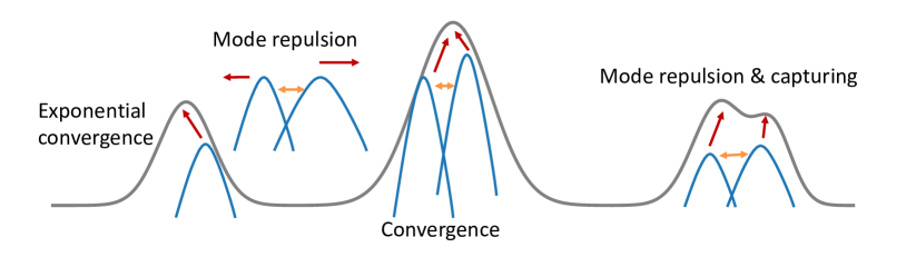
Figure 1: Schematic of properties of GMKI. The Grey curve represents the posterior distribution. Blue curves represent Gaussian components of the Gaussian mixture approximation. From left to right: Gaussian components can exhibit exponential convergence toward their respective Gaussian modes if these modes are well separated (see Proposition 7); the repulsion between distinct Gaussian components in the iteration of GMKI helps explore the space and capture multiple modes (see Section 5.1); when multiple Gaussian components converge towards a single Gaussian mode in the posterior distribution, they can provide a good approximation of the Gaussian mode (see Proposition 6); GMKI can capture multiple modes even when these modes are intertwined (see numerical examples in Section 6.1).

5.1 Exploration Effect

In the derivation of GMKI, the first step Eq. 27 is designed to approximate the exploration phase of the Fisher-Rao gradient flow Eq. 12a. In this subsection, we investigate whether the exploration effect still persists with the approximation made by GMKI. In fact, Eq. 27 tends to expand the distribution for exploration in the following two ways: (1) repulsion between Gaussian components; and (2) by an increase of the entropy. The repulsion effect can be understood through the following continuous time limit analysis. In this analysis we abuse notation, replacing the subscript $n$ in the discrete iterations by $t$, which equals $n\Delta t$ in the continuous limit of the means, covariances and weights of the the Gaussian mixture.

Proposition 3.

The continuous time limit $(\Delta t\rightarrow 0)$ of the exploration step Eq. 27 is

$$\dot{m}_{t,k} =-\int\mathcal{N}(\theta;m_{t,k},C_{t,k})(\theta-m_{t,k})\log\rho_{t}(\theta)\mathrm{d}\theta,$$ (31a)

$$\dot{C}_{t,k} =-\int\mathcal{N}(\theta;m_{t,k},C_{t,k})\Bigl{(}(\theta-m_{t,k})(\theta-m_{t,k})^{T}-C_{t,k}\Bigr{)}\log\rho_{t}(\theta)\mathrm{d}\theta,$$ (31b)

$$\dot{w}_{t,k} =-w_{t,k}\int\Bigl{[}\mathcal{N}(\theta;m_{t,k},C_{t,k})-\rho_{t}(\theta)\Bigr{]}\log\rho_{t}(\theta)\mathrm{d}\theta.$$ (31c)

Here $\rho_{t}(\theta)=\sum_{k=1}^{K}w_{t,k}\mathcal{N}(\theta;m_{t,k},C_{t,k})$.

The proof is in C.1. The continuous time limit of the evolution equation of the mean Eq. 31a suggests that, if $K\geq 2$, $m_{t,k}$ will move towards the direction where $\rho_{t}$ is small. Indeed, let’s consider a specific scenario where $N_{\theta}=1$, $K=2$ and $m_{t,1}<m_{t,2}$, In this case, we have that

$$\begin{split}\dot{m}_{t,1}&=-\int(\theta-m_{t,1})\mathcal{N}(\theta;m_{t,1},C_{t,1})\log\rho_{t}(\theta)\mathrm{d}\theta\\ &=-\int_{\theta>m_{t,1}}(\theta-m_{t,1})\mathcal{N}(\theta;m_{t,1},C_{t,1})(\log\rho_{t}(\theta)-\log\rho_{t}(2m_{t,1}-\theta))\mathrm{d}\theta<0,\end{split}$$ (32)

where the last inequality is due to the fact that

$$\log\rho_{t}(\theta)-\log\rho_{t}(2m_{t,1}-\theta)=\log\frac{w_{t,1}\mathcal{N}(\theta;m_{t,1},C_{t,1})+w_{t,2}\mathcal{N}(\theta;m_{t,2},C_{t,2})}{w_{t,1}\mathcal{N}(\theta;m_{t,1},C_{t,1})+w_{t,2}\mathcal{N}(2m_{t,1}-\theta;m_{t,2},C_{t,2})}.$$

The right hand side is non-negative, since when $\theta>m_{t,1}$, we have $|m_{t,2}-2m_{t,1}+\theta|=(m_{t,2}-m_{t,1})+(\theta-m_{t,1})>|m_{t,2}-\theta|$ and hence $\mathcal{N}(2m_{t,1}-\theta;m_{t,2},C_{t,2})<\mathcal{N}(\theta;m_{t,2},C_{t,2})$. Similarly, we can also establish that $\dot{m}_{t,2}>0$. Hence these two Gaussian means are repulsed.

We can also understand the exploration effect through the increase of the entropy; see Proposition 4. The proof can be found in C.2.

Proposition 4.

The entropy of the Gaussian mixture

$$\rho_{t}(\theta)=\sum_{k=1}^{K}w_{t,k}\mathcal{N}(\theta;m_{t,k},C_{t,k})$$

obtained from Eq. 31 is non-decreasing; indeed:

$$\begin{split}\frac{\mathrm{d}}{\mathrm{d}t}\int-\rho_{t}\log\rho_{t}\mathrm{d}\theta=&\sum_{k=1}^{K}\Bigl{(}\frac{\dot{w}_{t,k}^{2}}{w_{t,k}}+w_{t,k}\dot{m}_{t,k}^{T}C_{t,k}^{-1}\dot{m}_{t,k}+\frac{w_{t,k}}{2}{\rm tr}[\dot{C}_{t,k}^{T}C_{t,k}^{-1}\dot{C}_{t,k}C_{t,k}^{-1}]\Bigr{)}\geq 0.\end{split}$$ (33)

5.2 Convergence Analysis

To provide insights for the convergence of GMKI, we consider its continuous limit in time. Similar to Eq. 31, the continuous time limit of our GMKI is given in Proposition 5. The proof is in C.3.

Proposition 5.

The continuous time limit $(\Delta t\rightarrow 0)$ of the proposed GMKI defines the evolving Gaussian mixture measure

$$\rho_{t}(\theta)=\sum_{k=1}^{K}w_{t,k}\mathcal{N}(\theta;m_{t,k},C_{t,k})$$

where

$$\dot{m}_{t,k}= -C_{t,k}\int\mathcal{N}(\theta;m_{t,k},C_{t,k})\nabla_{\theta}\log\rho_{t}(\theta)\mathrm{d}\theta+\widehat{C}_{t,k}^{\theta x}\Sigma_{\nu}^{-1}(x-\widehat{x}_{t,k}),$$ (34a)

$$\dot{C}_{t,k}= -C_{t,k}\left(\int\mathcal{N}(\theta;m_{t,k},C_{t,k})\nabla_{\theta}\nabla_{\theta}\log\rho_{t}(\theta)\mathrm{d}\theta\right)C_{t,k}-\widehat{C}_{t,k}^{\theta x}\Sigma_{\nu}^{-1}{\widehat{C}_{t,k}^{T}},$$ (34b)

$$\dot{w}_{t,k}= -w_{t,k}\int\Bigl{[}\mathcal{N}(\theta;m_{t,k},C_{t,k})-\rho_{t}(\theta)\Bigr{]}\Bigl{[}\log\rho_{t}(\theta)+\Phi_{R}(\theta)\Bigr{]}\mathrm{d}\theta.$$ (34c)

Here

$$\begin{split}\widehat{x}_{t,k}=\mathbb{E}[\mathcal{F}(\theta)],\qquad\widehat{C}_{t,k}^{\theta x}=\mathrm{Cov}[\theta,\mathcal{F}(\theta)],\quad\textrm{with}\quad\theta\sim\mathcal{N}(m_{t,k},C_{t,k}).\end{split}$$ (35)

Remark 2.

We can also connect the continuous limit in Proposition 5 with the classical variational inference approach based on Gaussian mixtures. In fact, Eq. 34 can be obtained by combining natural gradient methods in the Gaussian mixture context and derivative-free Kalman approximation (similar to Remark 1); see C.8.  $\lozenge$

To gain insight into the convergence properties of the continuous flow, we first study Eq. 34 for the Gaussian posterior case; the proof can be found in C.4.

Proposition 6 (Linear inverse problems).

Assume $\mathcal{G}(\theta)=G\cdot\theta$ is linear, and the posterior is Gaussian with the form

$$\Phi_{R}(\theta)=\frac{1}{2}(\theta-m_{\rm post})^{T}C^{-1}_{\rm post}(\theta-m_{\rm post}).$$

Then, the KL divergence between the Gaussian mixture

$$\rho_{t}(\theta)=\sum_{k=1}^{K}w_{t,k}\mathcal{N}(\theta;m_{t,k},C_{t,k})$$

obtained from Eq. 34 and $\rho_{\rm post}$ is non-increasing:

$$\begin{split}\frac{\mathrm{d}}{\mathrm{d}t}\mathrm{KL}[\rho_{t}\|\rho_{\rm post}]=&-\sum_{k=1}^{K}\Bigl{(}\frac{\dot{w}_{t,k}^{2}}{w_{t,k}}+w_{t,k}\dot{m}_{t,k}^{T}C_{\rm post}^{-1}\dot{m}_{t,k}+\frac{w_{t,k}}{2}{\rm tr}[\dot{C}_{t,k}^{T}C_{t,k}^{-1}\dot{C}_{t,k}C_{t,k}^{-1}]\Bigr{)}\leq 0.\end{split}$$ (36)

Furthermore, the mean and Fisher information matrix of stationary points $\rho_{\infty}(\theta)=\sum_{k}w_{\infty,k}\mathcal{N}(\theta;m_{\infty,k},C_{\infty,k})$ satisfy that

$$\sum_{k=1}^{K}w_{\infty,k}m_{\infty,k}=m_{\rm post},\qquad\rm{FIM}[\rho_{\infty}]=\int\frac{\nabla_{\theta}\rho_{\infty}\nabla_{\theta}\rho_{\infty}^{T}}{\rho_{\infty}}\mathrm{d}\theta=C_{\rm post}^{-1}.$$ (37)

Remark 3.

Proposition 6 shows that, if the posterior is Gaussian, then the KL divergence of the GMKI is non-increasing in time. Furthermore the Gaussian mixture converges to a distribution $\rho_{\infty}$ from which the correct Gaussian statistics can be extracted. Nevertheless, from our current proof, it is not yet known whether $\rho_{\infty}$ converge to $\rho_{\rm post}$. We leave this question for future study.  $\lozenge$

Finally, we provide some formal analysis for the convergence of our GMKI in scenarios where the posterior distribution is a Gaussian mixture with the same number of components, namely

$$\rho_{\rm post}(\theta)=\sum_{k=1}^{K}w_{k}^{*}\mathcal{N}(\theta;m_{k}^{*},C_{k}^{*})\propto\exp(-\Phi_{R}(\theta))\quad\textrm{with}\inf_{1\leq k\leq K}\quad w_{k}^{*}>0.$$

For simplicity, we assume these Gaussian components are well separated. It is technical to give a precise definition of the well-separatedness of different Gaussian components; our argument here is purely formal and serves to provide insights for the behavior of GMKI. Suppose the $k$-th Gaussian component $\mathcal{N}(\theta;m_{k}(0),C_{k}(0))$ in GMKI is close to its corresponding mode (e.g., the $k$-th mode) of $\rho_{\rm post}$ while becoming well separated from other Gaussian components. In such case, we may simplify the continuous time limit Eq. 34 by neglecting the interaction between different Gaussian components. The simplified continuous time dynamics and its property are presented in Proposition 7, with derivations in C.5.

Proposition 7.

Consider the simplified continuous time dynamics

$$\dot{m}_{t,k}= \ C_{t,k}(C_{k}^{*})^{-1}(m_{k}^{*}-m_{t,k}),$$ (38a)

$$\dot{C}_{t,k}= \ C_{t,k}-C_{t,k}(C_{k}^{*})^{-1}C_{t,k},$$ (38b)

$$\dot{w}_{t,k}= \ w_{t,k}\bigl{(}\log w_{k}^{*}-\log w_{t,k}-\sum_{i=1}^{K}w_{t,i}(\log w_{i}^{*}-\log w_{t,i})\bigr{)}.$$ (38c)

Then, $m_{t,k}$, $C_{t,k}$, and $w_{t,k}$ will converge to $m_{k}^{*}$, $C_{k}^{*}$, and $w_{k}^{*}$ exponentially fast.

The proof of Proposition 7 can be found in C.6.

5.3 Affine Invariance

Sampling methods are said to be affine invariant if the algorithm is unchanged under any invertible affine mapping. It is a consequence of such a property that convergence rates across all Gaussians with positive covariance are the same. More generally affine invariant algorithms can be highly effective for highly anisotropic distributions [84, 85]. This effectiveness stems from their consistent behavior across all coordinate systems related by affine transformations. Specifically, the convergence properties of these methods can be understood by examining the optimal coordinate system, which minimizes anisotropy to the fullest extent, across all affine transformations. With this in mind, the following is of interest in relation to GMKI:

Proposition 8.

The continuous time limit in Proposition 5 is affine invariant.

The proof of Proposition 8 can be found in C.7.

5.4 Summary of Theoretical Analyses

Combining insights from Propositions 3, 6, 7 and 8, we anticipate that the repulsion between distinct Gaussian components will enable the proposed methodology GMKI to capture possible modes of the posterior distribution more effectively. Moreover, the algorithm will converge efficiently to modes of the posterior when these modes are well separated. Finally we note that the affine invariance property of the GMKI shows that it will be effective for the approximation of certain highly anisotropic distributions.

6 Numerical Study

In this section, we present numerical studies regarding the proposed GMKI algorithm. We focus on posterior distributions of unknown parameters or fields arising in inverse problems that may exhibit multiple modes. Three types of model problems are considered:

1. A one-dimensional bimodal problem: we use this problem as a proof-of-concept example. Our result demonstrates that the convergence rate remains unchanged no matter how overlapped the two modes are. This implies the independence of the convergence rate regarding potential barriers.

2. A two-dimensional bimodal problem: we use this benchmark problem, introduced in [61, 86], to compare GMKI with other sampling methods such as the Langevin dynamics and birth death process [24]. Our result shows that GMKI is not only more accurate but also more cost-effective for this specific problem.

3. A high-dimensional bimodal problem: we consider the inverse problem of recovering the initial velocity field of the Navier-Stokes flow. The problem is designed to have a symmetry which induces two modes in the posterior. We show that GMKI can capture both modes efficiently; this indicates GMKI’s potential for addressing multimodal problems in large-scale and high-dimensional applications.

Regarding the parameter of the GMKI algorithm (B), we will specify in detail the number of mixtures $K$ in each problem. For all experiments, we use the time-step size $\Delta t=0.5$ and adopt $J=1000$ points for the Monte Carlo estimation of Eq. 27.

6.1 One-Dimensional Bimodal Problem

We first consider the following 1D bimodal inverse problem, associated with forward model

$$y=\mathcal{G}(\theta)+\eta\quad\textrm{ with }\quad y=1,\quad\mathcal{G}(\theta)=\theta^{2}.$$

We assume the prior is $\rho_{\rm prior}\sim\mathcal{N}(3,2^{2})$ and consider different noise levels:

$$\textrm{Case A:}\quad\eta\sim\mathcal{N}(0,0.2^{2});$$

$$\textrm{Case B:}\quad\eta\sim\mathcal{N}(0,0.5^{2});$$

$$\textrm{Case C:}\quad\eta\sim\mathcal{N}(0,1.0^{2});$$

$$\textrm{Case D:}\quad\eta\sim\mathcal{N}(0,1.5^{2}).$$

Note that the overlap between these two modes is larger when the noise strength is larger. For case A, the two modes are well separated, and for case D, the two modes are nearly mingled.

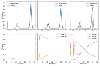
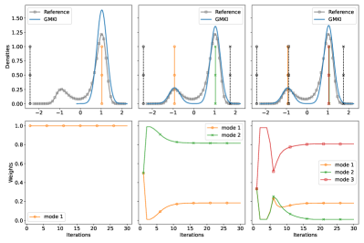
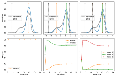
Figure 2: The one-dimensional bimodal problem with $\Sigma_{\eta}$ values of $0.2^{2}$ (top left), $0.5^{2}$ (top right), $1.0^{2}$ (bottom left), and $1.5^{2}$ (bottom right). Each panel displays, in the top row, the reference posterior distribution (grey square lines) and posterior distributions estimated by the GMKI (blue lines) at the $30$th iteration with mode number $K=1,\,2,\,3$ (from left to right) with mean $m_{k}$ (colored) and initial mean (black) of each Gaussian component marked. The bottom row shows weight estimations obtained by 1-mode GMKI, 2-mode GMKI and 3-mode GMKI (from left to right).

We apply GMKI with $K=1$, $2$, and $3$ modes, which are randomly initialized according to the prior distribution; we assign them equal weights. In each iteration, the GMKI algorithm requires $3$, $6$, and $9$ forward evaluations, respectively. The reference posterior distribution is obtained by evaluating the unnormalized posterior on a uniform grid and then normalizing it.

The results for different cases are reported from Fig. 2. The top row shows the reference posterior and posteriors approximated by GMKI at the $30$th iteration, and the bottom row shows the convergence of the weights. From left to right, we use different numbers of modes $K=1,\,2,\,3$. When $K=1$, we can only capture one mode, and this of course will not be weighted correctly since it will have weight one by construction; when $K=2$ or $3$, we can capture both modes. It is worth mentioning that GMKI converges in fewer than 30 iterations. The convergence behavior appears independent of the potential barrier. For case A, where the two modes are well separated, the approximated posteriors by GMKI with $K=2$ or $3$ match very well with the reference. This observation justifies our formal analysis in Proposition 7. For cases B,C,D, we observe that GMKI is capable of capturing both modes, however, some discrepancy will arise in the region where the modes overlap. These discrepancies persist when increasing the mode number in GMKI from $K=2$ to $K=3$.

6.2 Two-Dimensional Bimodal Problem

In this subsection, we consider the 2D bimodal inverse problem from [87, 86], associated with the forward model

$$y=\mathcal{G}(\theta)+\eta\quad\textrm{ with }\quad y=4.2297,\quad\mathcal{G}(\theta)=(\theta_{(1)}-\theta_{(2)})^{2}.$$

Here $\theta=[\theta_{(1)},\theta_{(2)}]^{T}$. We assume the noise distribution is $\eta\sim\mathcal{N}(0,I)$ and consider two different prior distributions:

$$\textrm{Case A:}\quad\rho_{\rm prior}\sim\mathcal{N}(0,I);$$

$$\textrm{Case B:}\quad\rho_{\rm prior}\sim\mathcal{N}([0.5,0]^{T},I).$$

For case A, the two modes are symmetric with respect to the line $\theta_{(1)}-\theta_{(2)}=0$, while for case B, the two modes are not symmetric.

We apply GMKI with $K=3$ modes, which are randomly initialized based on the prior distribution and we assign these components with equal weights. In each iteration, the algorithm requires $(2N_{\theta}+1)K=15$ forward evaluations. The reference posterior distribution is obtained by evaluating the unnormalized posterior on a uniform grid and then normalizing it. For both case A and case B, the estimated posterior distributions obtained by the GMKI at the $30$th iteration are presented in Figs. 3 and 4. We observe a strong correspondence with the reference, where in GMKI, mode 1 converges to one target mode, while mode 2 and mode 3 converge to another target mode.

Figure 3: Two-dimensional bimodal problem with $\rho_{\rm prior}\sim\mathcal{N}(0,I)$. From left to right: reference posterior distribution (left) and posterior distributions estimated by 3-modal GMKI (middle) at the 30th iteration (means $m_{k}$ (colored) and initial means (black) are marked) and BDLS-KL [24] (right) at the 1000th iteration.

Figure 4: Two-dimensional bimodal problem with $\rho_{\rm prior}\sim\mathcal{N}([0.5,0]^{T},I)$. From left to right: reference posterior distribution (left) and posterior distributions estimated by 3-modal GMKI (middle) at the 30th iteration (means $m_{k}$ (colored) and initial means (black) are marked) and BDLS-KL [24] (right) at the 1000th iteration.

As a comparison, the dervative-free affine-invariant Langevin dynamics (dfALDI) [60, 61] and derivative-free Bayesian inversion using multiscale dynamics [86] with $10^{6}$ iterations have been used for sampling the posterior distribution for case A. Their results are reported in [86, Figure 5], where dfALDI fails while multiscale dynamics can capture both modes but with wrong weights. The local preconditioner, which involves employing local empirical covariance with distance-dependent weights as introduced in [87], gives rise to an alternative derivative-free affine-invariant Langevin dynamics sampling approach. That approach notably enhances the sampling results in these scenarios. Moreover, for both case A and case B, we apply the BDLS-KL algorithm proposed in [24], which is a gradient-based sampler relying on the birth-death dynamics with kernel density estimators to approximate the Wasserstein-Fisher-Rao gradient flow. For the implementation of BDLS-KL, we use $\Delta t=10^{-2}$, $T=10$, ensemble size $J=10^{3}$, and the RBF kernel $k(x,x^{\prime})=\exp(\frac{1}{h}\lVert x-x^{\prime}\rVert^{2})$ with the bandwidth $h=\mathrm{med}^{2}/\log J$ adopted from [88]; here $\textrm{med}^{2}$ is the squared median of the pairwise Euclidean distance between the current particles. The results are shown in Figs. 3 and 4. For both cases, GMKI is not only more cost-effective but also more accurate compared to these existing approaches.

6.3 High-Dimensional Bimodal Problem: Navier Stokes Problem

Finally, we study the problem of recovering the initial vorticity field $\omega_{0}$ of a fluid flow from measurements at later times. The flow is described by the 2D Navier-Stokes equation on a periodic domain $D=[0,2\pi]\times[0,2\pi]$, which can be written in the vorticity-streamfunction $\omega-\psi$ formulation:

$$\begin{split}&\frac{\partial\omega}{\partial t}+(v\cdot\nabla)\omega-\nu\Delta\omega=\nabla\times f,\\ &\omega=-\Delta\psi\qquad\frac{1}{4\pi^{2}}\int\psi=0\qquad v=[\frac{\partial\psi}{\partial x_{2}},-\frac{\partial\psi}{\partial x_{1}}]^{T}+v_{b}.\end{split}$$ (39)

Here $v$ denotes the velocity vector, $\nu=0.01$ denotes the viscosity, $v_{b}=[0,2\pi]^{T}$ denotes the non-zero mean background velocity, and $f(x)=[0,\cos(4x_{(1)})]^{T}$ denotes the external forcing.

The problem is built to be spatially symmetric with respect to $x_{(1)}=\pi$. The source of the fluid is chosen such that

$$\nabla\times f([x_{(1)},x_{(2)}]^{T})=-\nabla\times f([2\pi-x_{(1)},x_{(2)}]^{T}).$$

The observations in the inverse problem are chosen as the difference of pointwise measurements of the vorticity value $\omega(\cdot)$

$$\omega([x_{(1)},x_{(2)}]^{T})-\omega([2\pi-x_{(1)},x_{(2)}]^{T})$$

at $56$ equidistant points in the left domain (see Figure 5), at $T=0.25$ and $T=0.5$, corrupted with observation error $\eta\sim\mathcal{N}(0,0.1^{2}I)$. Under this set-up, both $\omega_{0}([x_{(1)},x_{(2)}]^{T})$ and $-\omega_{0}([2\pi-x_{(1)},x_{(2)}]^{T})$ will lead to the same measurements. Thus the inverse problem will be at least bi-modal.

We assume the prior of $\omega_{0}(x,\theta)$ is a Gaussian field with covariance operator $C=(-\Delta)^{-2}$, subject to periodic boundary conditions, on the space of mean zero functions. The corresponding KL expansion of the initial vorticity field is given by

$$\omega_{0}(x,\theta)=\sum_{l\in K}\theta^{c}_{(l)}\sqrt{\lambda_{l}}\psi^{c}_{l}(x)+\theta^{s}_{(l)}\sqrt{\lambda_{l}}\psi^{s}_{l}(x),$$ (40)

where $\mathbb{L}=\{(l_{x},l_{y})|l_{x}+l_{y}>0\textrm{ or }(l_{x}+l_{y}=0\textrm{ and }l_{x}>0)\}$, and the eigenpairs are of the form

$$\psi^{c}_{l}(x)=\frac{\cos(l\cdot x)}{\sqrt{2}\pi}\quad\psi^{s}_{l}(x)=\frac{\sin(l\cdot x)}{\sqrt{2}\pi}\quad\lambda_{l}=\frac{1}{|l|^{4}},$$

and $\theta^{c}_{(l)},\theta^{s}_{(l)}\sim\mathcal{N}(0,2\pi^{2})$. The KL expansion Eq. 40 can be rewritten as a sum over positive integers rather than a lattice:

$$\omega_{0}(x,\theta)=\sum_{l=1}^{\infty}\theta_{(l)}\sqrt{\lambda_{l}}\psi_{l}(x),$$ (41)

where the eigenvalues $\lambda_{l}$ are in descending order. We truncate the expansion to the first $128$ terms and generate the true vorticity field $\omega_{0}(x;\theta_{\rm ref})$ with $\theta_{\rm ref}\in\mathbb{R}^{128}$; we aim to recover the parameter based on observation data.

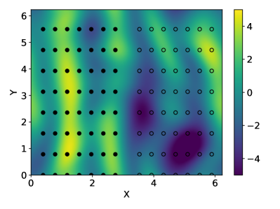
Figure 5: The vorticity field $\omega$ at $T=0.25$ and $T=0.5$ and observations $\omega([x_{(1)},x_{(2)}]^{T})-\omega([2\pi-x_{(1)},x_{(2)}]^{T})$ at $56$ equidistant points (solid black dots). Their mirroring points are marked (empty black dots).

We employ GMKI with $K=3$ modes, which are randomly initialized based on prior distribution with equal weights. Since we have $3$ modes and $N_{\theta}=128$, in each iteration, we require $(2N_{\theta}+1)K=771$ forward evaluations. We depict the true initial vorticity field $\omega_{0}(x;\theta_{\rm ref})$, its mirrored field (the mirroring of the velocity field induces the antisymmetry in the vorticity field) and the three recovered initial vorticity fields $\omega_{0}(x;m_{k})$ obtained by GMKI at the $50$th iteration in Fig. 6. Mode 1 captures the mirroring field of $\omega_{0}(x;\theta_{\rm ref})$ and mode 2 and mode 3 capture $\omega_{0}(x;\theta_{\rm ref})$. Figure 7 presents the relative errors of the vorticity field, the optimization errors $\Phi_{R}(m_{n,k})$, the Frobenius norm $\lVert C_{n,k}\rVert_{F}$ and the Gaussian mixture weights $w_{n,k}$ (from left to right). It shows that our GMKI converges in fewer than 50 iterations. Figure 8 displays the marginals of the estimated posterior distributions associated with the first $16$ theta coefficients obtained by GMKI. The marginal distributions exhibit clear bimodality, and the approximate posteriors have a high probability covering the true coefficients.

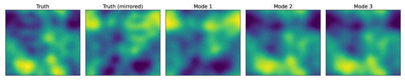
Figure 6: The true initial vorticity field $\omega_{0}(x;\theta_{\rm ref})$, and recovered initial vorticity fields $\omega_{0}(x;m_{k})$ obtained by GMKI.

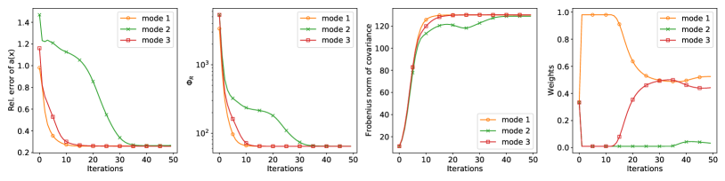
Figure 7: Navier-Stokes flow problem: the relative errors of the initial vorticity field, the optimization errors $\Phi_{R}(m_{n,k})$, the Frobenius norm $\lVert C_{n,k}\rVert_{F}$, and the Gaussian mixture weights $w_{n,k}$ (from left to right) for different modes.

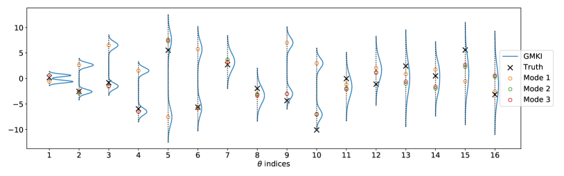
Figure 8: Navier-Stokes flow problem: the true Karhunen-Loeve expansion parameters $\theta_{(i)}$ (black crosses), and mean estimations of $\theta_{(i)}$ for each modes (circles) and the associated marginal distributions obtained GMKI at the $50$th iteration.

7 Conclusion

In this paper, we have presented a new framework for solving Bayesian inverse problems. The framework is based on the Fisher-Rao gradient flow. Within this framework, we introduce a novel approach, Gaussian mixture Kalman inversion (GMKI), which leverages Gaussian mixtures and Kalman’s methodology for numerical approximations of the the flow. GMKI is particularly useful when the posterior distribution has multiple modes and when the derivative of the forward model is not available or computationally expensive.

We derive the continuous time dynamics of the GMKI, showing its connection to Gaussian mixture variational inference, and studying its exploration effects and convergence properties. Our numerical experiments showcase GMKI’s capability in approximating posterior distributions with multiple modes. GMKI outperforms many existing Bayesian inference methods in terms of efficiency and accuracy.

There can be numerous avenues for future research. On the algorithmic side, it is of interest to refine the approximations employed by GMKI in regions where the mixture components overlap significantly; see the experimental results in Section 6.1. Moreover, although the Kalman methodology achieves a derivative-free implementation, it may suffer from degeneracy issues when the modes of the distribution concentrate on a low dimensional manifold; for a demonstration see D. Therefore, improving the derivative-free methodology in such a scenario is important for enhancing GMKI. On the theoretical side, a thorough analysis of the convergence of GMKI for general target distribution could offer valuable insights for its practical application.

Appendix A Convergence of the Exploration-Exploitation Scheme for the Fisher-Rao Gradient Flow

Proof of Proposition 2.

The solution of the Fisher-Rao gradient flow Eq. 3 has an analytical solution

$$\rho_{t}(\theta)=\frac{1}{Z_{t}}\rho_{0}(\theta)^{e^{-t}}\rho(\theta)^{1-e^{-t}},\quad\frac{\rho_{t}(\theta)}{\rho(\theta)}=\frac{1}{Z_{t}}\left(\frac{\rho_{0}(\theta)}{\rho(\theta)}\right)^{e^{-t}}.$$ (42)

where $Z_{t}$ is the normalization constant. The update Eq. 12 leads to

$$\rho_{n}(\theta)=\frac{1}{Z_{n}}\rho_{0}(\theta)^{(1-\Delta t)^{n}}\rho(\theta)^{1-(1-\Delta t)^{n}},\quad\frac{\rho_{n}(\theta)}{\rho(\theta)}=\frac{1}{Z_{n}}\left(\frac{\rho_{0}(\theta)}{\rho(\theta)}\right)^{(1-\Delta t)^{n}},$$ (43)

where $Z_{n}$ is the normalization constant. By comparing Eq. Eq. 43 and Eq. Eq. 42, we have

$$\rho_{n}(\theta)=\rho_{t}(\theta)\quad\text{for}\quad t=-n\log(1-\Delta t).$$

Bringing $t=-n\log(1-\Delta t)$ into Eq. 8 leads to

$$\mathrm{KL}[\rho_{n}\|\rho]=\mathrm{KL}[\rho_{-n\log(1-\Delta t)}\|\rho]\leq(2+B+eB)K(1-\Delta t)^{n},$$ (44)

when $-n\log(1-\Delta t)\geq\log((1+B)K)$. ∎

Appendix B Gaussian Mixture Kalman Inversion Algorithm

The detailed algorithm is presented in Algorithm 1.

Algorithm 1 Gaussian Mixture Kalman Inversion

Input: initial guess $\{w_{0,k},m_{0,k},C_{0,k}\}_{k=1}^{K}$, time-step size $\Delta t$, number of iterations $N$, number of particles $J$ for Monte Carlo, forward model $\mathcal{F}$

Output: final solution $\{w_{N,k},m_{N,k},C_{N,k}\}_{k=1}^{K}$

for $n\leftarrow 0$ to $N-1$ do

     for $k\leftarrow 1$ to $K$ do

         Sample $\{\theta^{j}\}_{j=1}^{J}\sim\mathcal{N}(\theta;m_{n,k},\frac{C_{n,k}}{1-\Delta t})$, first step update

$$\hat{w}_{n+1,k}=\frac{1}{J}\sum_{j=1}^{J}f_{n,k}(\theta^{j})$$

$$\widehat{m}_{n+1,k}=\frac{1}{\hat{w}_{n+1,k}J}\sum_{j=1}^{J}\theta^{j}f_{n,k}(\theta^{j})$$

$$\widehat{C}_{n+1,k}=\frac{1}{\hat{w}_{n+1,k}(J-1)}\sum_{j=1}^{J}(\theta^{j}-\widehat{m}_{n+1,k})(\theta^{j}-\widehat{m}_{n+1,k})^{T}f_{n,k}(\theta^{j})$$

     end for

     Normalize $\hat{w}_{n+1,k}:=\frac{\hat{w}_{n+1,k}}{\sum_{k=1}^{K}\hat{w}_{n+1,k}}$

     for $k\leftarrow 1$ to $K$ do $\triangleright$ Apply modified unscented transform [41, Eq. 37]

         Generate sigma-points $(a=\max\{\frac{1}{8},\frac{1}{2N_{\theta}}\})$

$$\theta_{k}^{0}=\widehat{m}_{n+1,k}$$

$$\theta_{k}^{j}=\widehat{m}_{n+1,k}+\frac{1}{\sqrt{2a}}[\sqrt{\widehat{C}_{n+1,k}}]_{j}\quad(1\leq j\leq N_{\theta})$$

$$\theta_{k}^{j+N_{\theta}}=\widehat{m}_{n+1,k}-\frac{1}{\sqrt{2a}}[\sqrt{\widehat{C}_{n+1,k}}]_{j}\quad(1\leq j\leq N_{\theta})$$

         Approximate the mean and covariance

$$\widehat{x}_{n+1,k}:=\mathcal{F}(\theta_{k}^{0})$$

$$\widehat{C}_{n+1,k}^{\theta x}:=\sum_{j=1}^{2N_{\theta}}a(\theta_{k}^{j}-\widehat{m}_{n+1,k})(\mathcal{F}(\theta_{k}^{j})-\widehat{x}_{n+1,k})^{T}$$

$$\widehat{C}_{n+1,k}^{xx}:=\sum_{j=1}^{2N_{\theta}}a(\mathcal{F}(\theta_{k}^{j})-\widehat{x}_{n+1,k})(\mathcal{F}(\theta_{k}^{j})-\widehat{x}_{n+1,k})^{T}+\frac{\Sigma_{\nu}}{\Delta t}$$

         Second step update

$$\begin{split}m_{n+1,k}&=\widehat{m}_{n+1,k}+\widehat{C}_{n+1,k}^{\theta x}(\widehat{C}_{n+1,k}^{xx})^{-1}(x-\widehat{x}_{n+1,k})\\ C_{n+1,k}&=\widehat{C}_{n+1,k}-\widehat{C}_{n+1,k}^{\theta x}(\widehat{C}_{n+1,k}^{xx})^{-1}{\widehat{C}_{n+1,k}^{{\theta x}^{T}}}\\ w_{n+1,k}&=\hat{w}_{n+1,k}e^{-\Delta t\Phi_{R}(\theta_{k}^{0})}\end{split}$$

     end for

     Normalize ${w}_{n+1,k}:=\frac{{w}_{n+1,k}}{\sum_{k=1}^{K}{w}_{n+1,k}}$

end for

Appendix C Theoretical Studies About GMKI

C.1 Proof of Proposition 3

Update equation Eq. 27 and the normalization of weights $\{\hat{w}_{n+1,k}\}_{k}$ can be combined and rewritten as

$$\hat{w}_{n+1,k}=\frac{w_{n,k}\int\mathcal{N}(\theta;m_{n,k},C_{n,k})\rho_{n}^{-\Delta t}\mathrm{d}\theta}{\int\rho_{n}^{1-\Delta t}\mathrm{d}\theta},$$ (45a)

$$\widehat{m}_{n+1,k}=\frac{\int\theta\mathcal{N}(\theta;m_{n,k},C_{n,k})\rho_{n}^{-\Delta t}\mathrm{d}\theta}{\int\mathcal{N}(\theta;m_{n,k},C_{n,k})\rho_{n}^{-\Delta t}\mathrm{d}\theta},$$ (45b)

$$\widehat{C}_{n+1,k}=\frac{\int(\theta-\widehat{m}_{n+1,k})(\theta-\widehat{m}_{n+1,k})^{T}\mathcal{N}(\theta;m_{n,k},C_{n,k})\rho_{n}^{-\Delta t}\mathrm{d}\theta}{\int\mathcal{N}(\theta;m_{n,k},C_{n,k})\rho_{n}^{-\Delta t}\mathrm{d}\theta}.$$ (45c)

Now we derive the continuous time limit of the exploration step; we ignore the hat notation for simplicity.

$$\frac{\hat{w}_{n+1,k}-w_{n,k}}{\Delta t} =w_{n,k}\frac{\int\Bigl{[}\mathcal{N}(\theta;m_{n,k},C_{n,k})-\rho_{n}\Bigr{]}\rho_{n}^{-\Delta t}\mathrm{d}\theta}{\Delta t\int\rho_{n}^{1-\Delta t}\mathrm{d}\theta}$$ (46)

$$=w_{n,k}\frac{\int\Bigl{[}\mathcal{N}(\theta;m_{n,k},C_{n,k})-\rho_{n}\Bigr{]}(1-\Delta t\log\rho_{n})\mathrm{d}\theta}{\Delta t}+O(\Delta t)$$

$$=-w_{n,k}\int\Bigl{[}\mathcal{N}(\theta;m_{n,k},C_{n,k})-\rho_{n}\Bigr{]}\log\rho_{n}\mathrm{d}\theta+O(\Delta t).$$

Therefore the continuous limit can be written as

$$\dot{w}_{t,k}=-w_{t,k}\int\Bigl{[}\mathcal{N}(\theta;m_{t,k},C_{t,k})-\rho_{t}(\theta)\Bigr{]}\log\rho_{t}(\theta)\mathrm{d}\theta\,.$$

Similarly, for $m_{n,k}$ we have

$$\frac{\widehat{m}_{n+1,k}-m_{n,k}}{\Delta t} =\frac{\int(\theta-m_{n,k})\mathcal{N}(\theta;m_{n,k},C_{n,k})\rho_{n}^{-\Delta t}\mathrm{d}\theta}{\Delta t\int\mathcal{N}(\theta;m_{n,k},C_{n,k})\rho_{n}^{-\Delta t}\mathrm{d}\theta}$$ (47)

$$=\frac{\int(\theta-m_{n,k})\mathcal{N}(\theta;m_{n,k},C_{n,k})(1-\Delta t\log\rho_{n})\mathrm{d}\theta}{\Delta t}+O(\Delta t)$$

$$=-\int\mathcal{N}(\theta;m_{n,k},C_{n,k})(\theta-m_{n,k})\log\rho_{n}(\theta)\mathrm{d}\theta+O(\Delta t)$$

$$=-C_{n,k}\int\mathcal{N}(\theta;m_{n,k},C_{n,k})\nabla_{\theta}\log\rho_{n}(\theta)\mathrm{d}\theta+O(\Delta t),$$

where in the last identity, we used integration by parts; it is also known as the Stein’s identity. Thus the continuous limit is

$$\dot{m}_{t,k}=-\int\mathcal{N}(\theta;m_{t,k},C_{t,k})(\theta-m_{t,k})\log\rho_{t}(\theta)\mathrm{d}\theta.$$

Finally, for $C_{n,k}$, we have

$$\frac{\widehat{C}_{n+1,k}-C_{n,k}}{\Delta t}$$ (48)

$$= \frac{\int\Bigl{[}(\theta-\widehat{m}_{n+1,k})(\theta-\widehat{m}_{n+1,k})^{T}-C_{n,k}\Bigr{]}\mathcal{N}(\theta;m_{n,k},C_{n,k})\rho_{n}^{-\Delta t}\mathrm{d}\theta}{\Delta t\int\mathcal{N}(\theta;m_{n,k},C_{n,k})\rho_{n}^{-\Delta t}\mathrm{d}\theta}$$

$$= \frac{\int\Bigl{[}(\theta-\widehat{m}_{n,k})(\theta-\widehat{m}_{n,k})^{T}-C_{n,k}\Bigr{]}\mathcal{N}(\theta;m_{n,k},C_{n,k})(1-\Delta t\rho_{n})\mathrm{d}\theta}{\Delta t}+O(\Delta t)$$

$$= -\int\Bigl{[}(\theta-{m}_{n,k})(\theta-m_{n,k})^{T}-C_{n,k}\Bigr{]}\mathcal{N}(\theta;m_{n,k},C_{n,k})\rho_{n}\mathrm{d}\theta+O(\Delta t)$$

$$=-C_{n,k}\int\mathcal{N}(\theta;m_{n,k},C_{n,k})\nabla_{\theta}\nabla_{\theta}\log\rho_{n}\mathrm{d}\theta C_{n,k}+O(\Delta t),$$

which leads to the desired continuous limit stated in the proposition.

C.2 Proof of Proposition 4

The evolution equation of the entropy of $\rho_{t}$ is

$$\begin{split}&\frac{\mathrm{d}}{\mathrm{d}t}\int-\rho_{t}\log\rho_{t}\mathrm{d}\theta=-\int\frac{\mathrm{d}\rho_{t}}{\mathrm{d}t}\log\rho_{t}\mathrm{d}\theta\\ =&-\sum_{k}\dot{w}_{t,k}\int\mathcal{N}(\theta;m_{t,k},C_{t,k})\log\rho_{t}\mathrm{d}\theta\\ &-\sum_{k}w_{k}\dot{m}_{t,k}^{T}C_{t,k}^{-1}\int(\theta-m_{t,k})\mathcal{N}(\theta;m_{t,k},C_{t,k})\log\rho_{t}\mathrm{d}\theta\\ &-\sum_{k}\frac{w_{t,k}}{2}{\rm tr}\Bigl{[}\dot{C}_{t,k}^{T}\int\bigl{(}C_{t,k}^{-1}(\theta-m_{t,k})(\theta-m_{t,k})^{T}C_{t,k}^{-1}-C_{t,k}^{-1}\bigr{)}\mathcal{N}(\theta;m_{t,k},C_{t,k})\log\rho_{t}\mathrm{d}\theta\Bigr{]}\\ =&\sum_{k}\Bigl{(}\frac{\dot{w}_{t,k}^{2}}{w_{t,k}}+w_{t,k}\dot{m}_{t,k}^{T}C_{t,k}^{-1}\dot{m}_{t,k}+\frac{w_{t,k}}{2}{\rm tr}\Bigl{[}\dot{C}_{t,k}C_{t,k}^{-1}\dot{C}_{t,k}C_{t,k}^{-1}\Bigr{]}\Bigr{)}.\end{split}$$ (49)

Here we have used the fact $\int\frac{\mathrm{d}\rho_{t}}{\mathrm{d}t}\mathrm{d}\theta=0$ in the first identity. And in the second identity we used the fact that $\sum_{k}\dot{w}_{t,k}=0$ and used the continuous time limit equations Eq. 31.

C.3 Proof of Proposition 5

Combining Proposition 3 and Eq. 29 leads to the following

$$\begin{split}&\frac{m_{n+1,k}-m_{n,k}}{\Delta t}\\ =&\frac{\widehat{m}_{n+1,k}-m_{n,k}}{\Delta t}+\frac{\widehat{C}_{n+1,k}^{\theta x}(\widehat{C}_{n+1,k}^{xx})^{-1}(x-\widehat{x}_{n+1,k})}{\Delta t}\\ =&-C_{n,k}\int\mathcal{N}(\theta;m_{n,k},C_{n,k})\nabla_{\theta}\log\rho_{n}(\theta)\mathrm{d}\theta+\widehat{C}_{n,k}^{\theta x}\Sigma_{\nu}^{-1}(x-\widehat{x}_{n,k})+O(\Delta t).\\ &\frac{C_{n+1,k}-C_{n,k}}{\Delta t}\\ =&\frac{\widehat{C}_{n+1,k}-C_{n,k}}{\Delta t}-\frac{\widehat{C}_{n+1,k}^{\theta x}(\widehat{C}_{n+1,k}^{xx})^{-1}{\widehat{C}_{n+1,k}^{{\theta x}^{T}}}}{\Delta t}\\ =&-C_{n,k}\int\mathcal{N}(\theta;m_{n,k},C_{n,k})\nabla_{\theta}\nabla_{\theta}\log\rho_{n}(\theta)\mathrm{d}\theta C_{n,k}-\widehat{C}_{n,k}^{\theta x}\Sigma_{\nu}^{-1}{\widehat{C}_{n,k}^{{\theta x}^{T}}}+O(\Delta t).\end{split}$$ (50)

Using the above formula, we obtain the continuous limit. For the weights, we have

$$w_{n+1,k}=\frac{\hat{w}_{n+1,k}\int\mathcal{N}(\theta;\widehat{m}_{n+1,k},\widehat{C}_{n+1,k})e^{-\Delta t\Phi_{R}(\theta)}\mathrm{d}\theta}{\int\hat{\rho}_{n+1}e^{-\Delta t\Phi_{R}(\theta)}\mathrm{d}\theta}.$$ (51a)

Therefore,

$$\begin{split}&\frac{w_{n+1,k}-w_{n,k}}{\Delta t}=\frac{w_{n+1,k}-\hat{w}_{n,k}}{\Delta t}+\frac{\hat{w}_{n+1,k}-w_{n,k}}{\Delta t}\\ =&\hat{w}_{n+1,k}\frac{\int\bigl{[}\mathcal{N}(\theta;\widehat{m}_{n+1,k},\widehat{C}_{n+1,k})-\hat{\rho}_{n+1}\bigr{]}e^{-\Delta t\Phi_{R}}\mathrm{d}\theta}{\Delta t\int\hat{\rho}_{n+1}e^{-\Delta t\Phi_{R}}\mathrm{d}\theta}+\frac{\hat{w}_{n+1,k}-w_{n,k}}{\Delta t}+O(\Delta t)\\ =&\hat{w}_{n+1,k}\frac{\int\bigl{[}\mathcal{N}(\theta;\widehat{m}_{n+1,k},\widehat{C}_{n+1,k})-\hat{\rho}_{n+1}\bigr{]}(1-\Delta t\Phi_{R})\mathrm{d}\theta}{\Delta t}+\frac{\hat{w}_{n+1,k}-w_{n,k}}{\Delta t}+O(\Delta t)\\ =&-w_{n,k}\int\Bigl{[}\mathcal{N}(\theta;m_{n,k},C_{n,k})-\rho_{n}\Bigr{]}(\log\rho_{n}+\Phi_{R})\mathrm{d}\theta+O(\Delta t),\end{split}$$ (52)

from which we readily obtain the continuous limit for the equation of the weights. Here in the last step we used the result in C.1.

C.4 Proof of Proposition 6

Under the Gaussian posterior assumption (i.e. $\Phi_{R}$ is quadratic) and based on the formula in (24) and (25), we get

$$\widehat{C}_{t,k}^{\theta x}\Sigma_{\nu}^{-1}(x-\widehat{x}_{t,k})=-C_{t,k}\int\mathcal{N}(\theta;m_{t,k},C_{t,k})\nabla_{\theta}\Phi_{R}\mathrm{d}\theta,$$ (53)

$$\widehat{C}_{t,k}^{\theta x}\Sigma_{\nu}^{-1}{\widehat{C}_{t,k}^{T}}=C_{t,k}\left(\int\mathcal{N}(\theta;m_{t,k},C_{t,k})\nabla_{\theta}\nabla_{\theta}\Phi_{R}\mathrm{d}\theta\right)C_{t,k}^{T}.$$ (54)

Bringing Eq. 53 into the continuous time dynamics Eq. 34 and using integration by parts (also known as Stein’s identities) leads to

$$\dot{m}_{t,k}= -C_{t,k}\int\mathcal{N}(\theta;m_{t,k},C_{t,k})\nabla_{\theta}\bigl{(}\log\rho_{t}+\Phi_{R}\bigr{)}\mathrm{d}\theta$$

$$= -\int\mathcal{N}(\theta;m_{t,k},C_{t,k})(\theta-m_{t,k})\bigl{(}\log\rho_{t}+\Phi_{R}\bigr{)}\mathrm{d}\theta,$$ (55a)

$$\dot{C}_{t,k}= -\int\mathcal{N}(\theta;m_{t,k},C_{t,k})\nabla_{\theta}\nabla_{\theta}\bigl{(}\log\rho_{t}+\Phi_{R}\bigr{)}\mathrm{d}\theta$$

$$= -\int\mathcal{N}(\theta;m_{t,k},C_{t,k})\Bigl{(}(\theta-m_{t,k})(\theta-m_{t,k})^{T}-C_{t,k}\Bigr{)}\bigl{(}\log\rho_{t}+\Phi_{R}\bigr{)}\mathrm{d}\theta,$$ (55b)

$$\dot{w}_{t,k}= -w_{t,k}\int\Bigl{[}\mathcal{N}(\theta;m_{t,k},C_{t,k})-\rho_{t}\Bigr{]}\Bigl{[}\log\rho_{t}+\Phi_{R}\Bigr{]}\mathrm{d}\theta.$$ (55c)

The evolution equation of the KL divergence between $\rho_{t}$ and $\rho_{\rm post}$ is then

$$\begin{split}&\frac{\mathrm{d}}{\mathrm{d}t}\mathrm{KL}[\rho_{t}\|\rho_{\rm post}]\\ =&\frac{\mathrm{d}}{\mathrm{d}t}\int\rho_{t}\log\Bigl{(}\frac{\rho_{t}}{\rho_{\rm post}}\Bigr{)}\mathrm{d}\theta=\int\frac{\mathrm{d}\rho_{t}}{\mathrm{d}t}\bigl{(}\log\rho_{t}+\Phi_{R}\bigr{)}\mathrm{d}\theta\\ =&\sum_{k}\dot{w}_{t,k}\int\mathcal{N}(\theta;m_{t,k},C_{t,k})\bigl{(}\log\rho_{t}+\Phi_{R}\bigr{)}\mathrm{d}\theta\\ &-\sum_{k}w_{k}\dot{m}_{t,k}^{T}C_{t,k}^{-1}\int(\theta-m_{t,k})\mathcal{N}(\theta;m_{t,k},C_{t,k})\bigl{(}\log\rho_{t}+\Phi_{R}\bigr{)}\mathrm{d}\theta\\ &+\sum_{k}\frac{w_{t,k}}{2}{\rm tr}\Bigl{[}\dot{C}_{t,k}^{T}\int\bigl{(}C_{t,k}^{-1}(\theta-m_{t,k})(\theta-m_{t,k})^{T}C_{t,k}^{-1}-C_{t,k}^{-1}\bigr{)}\mathcal{N}(\theta;m_{t,k},C_{t,k})\bigl{(}\log\rho_{t}+\Phi_{R}\bigr{)}\mathrm{d}\theta\Bigr{]}\\ =&-\sum_{k}\Bigl{(}\frac{\dot{w}_{t,k}^{2}}{w_{t,k}}+w_{t,k}\dot{m}_{t,k}^{T}C_{t,k}^{-1}\dot{m}_{t,k}+\frac{w_{t,k}}{2}{\rm tr}\Bigl{[}\dot{C}_{t,k}C_{t,k}^{-1}\dot{C}_{t,k}C_{t,k}^{-1}\Bigr{]}\Bigr{)}.\end{split}$$ (56)

Here in the last identity, we used the equation of the continuous time dynamics in (55) to simplify the formula.

Consider any stationary point $\rho_{\infty}=\sum_{k}w_{k,\infty}\mathcal{N}(\theta;m_{k,\infty},C_{k,\infty})$ with nonzero $w_{k,\infty}$. The stationary point condition for the mean $m_{k,\infty}$ (55a) is

$$\int\mathcal{N}(\theta;m_{k,\infty},C_{k,\infty})\nabla_{\theta}\log\rho_{\infty}\mathrm{d}\theta=-C_{\rm post}^{-1}(m_{k,\infty}-m_{\rm post}),$$ (57)

where we used that $\int\mathcal{N}(\theta;m_{\infty,k},C_{\infty,k})\nabla_{\theta}\Phi_{R}\mathrm{d}\theta=C_{\rm post}^{-1}(m_{k,\infty}-m_{\rm post})$. The stationary point condition for the covariance $C_{k,\infty}$ (55b) is

$$\int\mathcal{N}(\theta;m_{k,\infty},C_{k,\infty})\nabla_{\theta}\nabla_{\theta}\log\rho_{\infty}\mathrm{d}\theta=-C_{\rm post}^{-1},$$ (58)

where we used that $\int\mathcal{N}(\theta;m_{\infty,k},C_{\infty,k})\nabla_{\theta}\nabla_{\theta}\Phi_{R}\mathrm{d}\theta=C_{\rm post}^{-1}$. Multiplying Eq. 57 and Eq. 58 by $w_{k,\infty}$ and summing the results yields

$$m_{\rm post}-\sum_{k}w_{k,\infty}m_{k,\infty}=C_{\rm post}\int\sum_{k}w_{k,\infty}\mathcal{N}(\theta;m_{k,\infty},C_{k,\infty})\nabla_{\theta}\log\rho_{\infty}\mathrm{d}\theta=0,$$ (59)

$$C_{\rm post}^{-1}=-\int\sum w_{k,\infty}\mathcal{N}(\theta;m_{k,\infty},C_{k,\infty})\nabla_{\theta}\nabla_{\theta}\log\rho_{\infty}\mathrm{d}\theta={\rm FIM}[\rho_{\infty}].$$

C.5 Derivation of the Simplified Continuous Time Dynamics Eq. 38

In this section, we formally derive Eq. 38, assuming these Gaussian components in $\rho_{\rm post}$ are well separated. When $\theta$ is close to $m_{k}^{*}$, one may make the following approximation

$$\Phi_{R}(\theta)=\log\rho_{\rm post}(\theta)\approx-\log\mathcal{N}(\theta,m_{k}^{*},C_{k}^{*})-\log(w_{k}^{*}).$$ (60)

Combining the definition of $\Phi_{R}$ in Eq. 18 with Eq. 60 leads to that

$$-\frac{1}{2}(x-\mathcal{F}(\theta))^{T}\Sigma_{\nu}^{-1}(x-\mathcal{F}(\theta))\approx-\frac{1}{2}(\theta-m_{k}^{*})^{T}C_{k}^{*^{-1}}(\theta-m_{k}^{*})+\textrm{constant}.$$ (61)

This implies that $\mathcal{F}(\theta)$ is approximately locally linear around $m=m_{k}^{*}$ with $\mathcal{F}(\theta)\approx F_{k}\theta+c$, such that $F_{k}^{T}\Sigma_{\nu}^{-1}F_{k}=C_{k}^{*^{-1}}$ and $C_{k}^{*}F_{k}^{T}\Sigma_{\nu}^{-1}(x-c)=m_{k}^{*}$. Based on the above derivation, when the $k$-the component $\mathcal{N}(\theta;m_{t,k},C_{t,k})$ in the Gaussian mixture approximation is concentrating around $m_{k}^{*}$, the expectation and covariance in the continuous time limit of the proposed GMKI (35) can be approximated as

$$\widehat{x}_{t,k} =\mathbb{E}[\mathcal{F}(\theta)]\approx\mathbb{E}[F_{k}\theta+c]=F_{k}m_{t,k}+c,$$ (62a)

$$\widehat{C}_{t,k}^{\theta x} =\textrm{Cov}\bigl{[}\theta,\mathcal{F}(\theta)\bigr{]}\approx\mathbb{E}\bigl{[}\bigl{(}\theta-m_{t,k}\bigr{)}\otimes\bigl{(}F_{k}(\theta-m_{t,k})\bigr{)}\bigr{]}=C_{t,k}F_{k}^{T}.$$ (62b)

Here the expectation are taken with respect to $\mathcal{N}(\theta;m_{t,k},C_{t,k})$.

Now we will simplify Eq. 34 by neglecting the interaction between well separated Gaussian components to obtain Eq. 38. For the mean evolution equation (34a), we have

$$\begin{split}\dot{m}_{t,k}\approx&-C_{t,k}\int\mathcal{N}(\theta;m_{t,k},C_{t,k})\nabla_{\theta}\log\bigl{(}w_{k}\mathcal{N}(\theta;m_{t,k},C_{t,k})\bigr{)}\mathrm{d}\theta+\widehat{C}_{t,k}^{\theta x}\Sigma_{\nu}^{-1}(x-\widehat{x}_{t,k})\\ =&\widehat{C}_{t,k}^{\theta x}\Sigma_{\nu}^{-1}(x-\widehat{x}_{t,k})\\ \approx&C_{t,k}(C_{k}^{*})^{-1}(m_{k}^{*}-m_{t,k}).\end{split}$$ (63)

The first approximation is obtained by substituting $\log\rho_{t}$ with $\log(w_{k}\mathcal{N}(\theta;m_{t,k},C_{t,k}))$, due to the well separateness assumption; the resulting integral is zero so leads to the second identity. The third approximation is obtained by using Eq. 62 and the relation $F_{k}^{T}\Sigma_{\nu}^{-1}F_{k}=C_{k}^{*^{-1}}$ and $C_{k}^{*}F_{k}^{T}\Sigma_{\nu}^{-1}(x-c)=m_{k}^{*}$.

For the covariance evolution equation (34b), similarly we have

$$\begin{split}\dot{C}_{t,k}\approx&-C_{t,k}\left(\int\mathcal{N}(\theta;m_{t,k},C_{t,k})\nabla_{\theta}\nabla_{\theta}\log\bigl{(}w_{k}\mathcal{N}(\theta;m_{t,k},C_{t,k})\bigr{)}\mathrm{d}\theta\right)C_{t,k}-\widehat{C}_{t,k}^{\theta x}\Sigma_{\nu}^{-1}{\widehat{C}_{t,k}^{T}}\\ =&\ C_{t,k}-\widehat{C}_{t,k}^{\theta x}\Sigma_{\nu}^{-1}{\widehat{C}_{t,k}^{T}}\\ =&\ C_{t,k}-C_{t,k}(C_{k}^{*})^{-1}C_{t,k}.\end{split}$$ (64)

The first approximation is obtained by by substituting $\log\rho_{t}$ with $\log(w_{k}\mathcal{N}(\theta;m_{t,k},C_{t,k}))$. The third approximation is obtained by using Eq. 62.

Finally, for the weight evolution equation (34c), using the formula $\rho_{t}(\theta)=\sum_{i}\int w_{t,i}\mathcal{N}(\theta;m_{t,i},C_{t,i})$, we get

$$\begin{split}\dot{w}_{t,k}=&-w_{t,k}\int\mathcal{N}(\theta;m_{t,k},C_{t,k})\log\rho_{t}(\theta)\mathrm{d}\theta+w_{t,k}\sum_{i}\int w_{t,i}\mathcal{N}(\theta;m_{t,i},C_{t,i})\log\rho_{t}(\theta)\mathrm{d}\theta\\ &-w_{t,k}\int\mathcal{N}(\theta;m_{t,k},C_{t,k})\Phi_{R}(\theta)\mathrm{d}\theta+w_{t,k}\sum_{i}\int w_{t,i}\mathcal{N}(\theta;m_{t,i},C_{t,i})\Phi_{R}(\theta)\mathrm{d}\theta\\ \approx&-w_{t,k}\int\mathcal{N}(\theta;m_{t,k},C_{t,k})\log[w_{t,k}\mathcal{N}(\theta;m_{t,k},C_{t,k})]\mathrm{d}\theta\\ &+w_{t,k}\sum_{i}\int w_{t,i}\mathcal{N}(\theta;m_{t,i},C_{t,i})\log[w_{t,i}\mathcal{N}(\theta;m_{t,i},C_{t,i})]\mathrm{d}\theta\\ &+w_{t,k}\int\mathcal{N}(\theta;m_{t,k},C_{t,k})\Bigl{(}\log\mathcal{N}(\theta,m_{k}^{*},C_{k}^{*})+\log(w_{k}^{*})\Bigr{)}\mathrm{d}\theta\\ &-w_{t,k}\sum_{i}\int w_{t,i}\mathcal{N}(\theta;m_{t,i},C_{t,i})\Bigl{(}\log\mathcal{N}(\theta,m_{i}^{*},C_{i}^{*})+\log(w_{i}^{*})\Bigr{)}\mathrm{d}\theta\\ =&w_{t,k}\bigl{(}\log w_{k}^{*}-\log w_{t,k}-\sum_{i}w_{t,i}(\log w_{i}^{*}-\log w_{t,i})\bigr{)}.\end{split}$$ (65)

The first approximation is obtained by substituting $\log\rho_{t}$ with $\log(w_{k}\mathcal{N}(\theta;m_{t,k},C_{t,k}))$ and using Eq. 60 for approximating $\Phi_{R}(\theta)$. Combining Eqs. 63, 64 and 65 leads to the simplified continuous time dynamics Eq. 38.

C.6 Proof of Proposition 7

The mean, covariance and weight evolution equations Eqs. 38a, 38b and 38c admit analytical solutions

$$m_{t,k}=m_{k}^{*}+e^{-t}\Bigl{(}(1-e^{-t})C_{k}^{*^{-1}}+e^{-t}C_{k}(0)^{-1}\Bigr{)}^{-1}C_{k}(0)^{-1}\bigl{(}m_{k}(0)-m_{k}^{*}\bigr{)},$$ (66a)

$$C_{t,k}^{-1}=C_{k}^{*^{-1}}+e^{-t}(C_{k}(0)^{-1}-C_{k}^{*^{-1}}),$$ (66b)

$$w_{k}=\frac{w_{k}^{*}\Bigl{(}\frac{w_{k}(0)}{w_{k}^{*}}\Bigr{)}^{e^{-t}}}{\sum_{i}w_{i}^{*}\Bigl{(}\frac{w_{i}(0)}{w_{i}^{*}}\Bigr{)}^{e^{-t}}}.$$ (66c)

They will converge to $m_{k}^{*}$, $C_{k}^{*}$ and $w_{k}^{*}$ exponentially fast.

C.7 Proof of Proposition 8

Consider any invertible affine mapping $\varphi:\theta\rightarrow\widetilde{\theta}=A\theta+b$, and define corresponding vector and matrix transformations

$$\widetilde{m}_{t,k}=Am_{t,k}+b\quad\widetilde{C}_{t,k}=AC_{t,k}A^{T},$$

density transformations

$${\widetilde{\rho}}(\widetilde{\theta})=\varphi\#\rho(\theta)=\rho(A^{-1}(\widetilde{\theta}-b))|A|^{-1}\quad\mathcal{N}(\widetilde{\theta};\widetilde{m}_{t,k},\widetilde{C}_{t,k})=\mathcal{N}(\theta;m_{t,k},C_{t,k})|A|^{-1},$$

function transformations

$$\widetilde{\mathcal{F}}(\widetilde{\theta})=\mathcal{F}(A^{-1}(\widetilde{\theta}-b))\quad\quad\widetilde{\Phi}_{R}(\widetilde{\theta})=\Phi_{R}(A^{-1}(\widetilde{\theta}-b)),$$

and their related expectation and covariance

$$\widetilde{x}_{t,k}=\mathbb{E}[\widetilde{\mathcal{F}}(\widetilde{\theta})],\qquad\widetilde{C}^{\theta x}_{t,k}=\mathrm{Cov}[\widetilde{\theta},\widetilde{\mathcal{F}}(\widetilde{\theta})],\quad\textrm{with}\quad\widetilde{\theta}\sim\mathcal{N}(\widetilde{m}_{t,k},\widetilde{C}_{t,k}),$$

then we have

$$\begin{split}&\nabla_{\widetilde{\theta}}\log\widetilde{\rho}(\widetilde{\theta})=A^{-T}\nabla_{\theta}\log\rho(\theta)\qquad\nabla_{\widetilde{\theta}}\nabla_{\widetilde{\theta}}\log\widetilde{\rho}(\widetilde{\theta})=A^{-T}\nabla_{\theta}\log\rho(\theta)A^{-1}\\ &\widetilde{x}_{t,k}=\widehat{x}_{t,k}\qquad\widetilde{C}_{t,k}^{\theta x}=A\widehat{C}_{t,k}^{\theta x}.\end{split}$$ (67)

The evolution equations of $\widetilde{m}_{t,k}$, $\widetilde{C}_{t,k}$, $w_{t,k}$ in Eq. 34 can be rewritten as

$$\dot{\widetilde{m}}_{t,k}= -AC_{t,k}\int\mathcal{N}(\theta;m_{t,k},C_{t,k})\nabla_{\theta}\log\rho_{t}(\theta)\mathrm{d}\theta+A\widehat{C}_{t,k}^{\theta x}\Sigma_{\nu}^{-1}(x-\widehat{x}_{t,k}),$$

$$= -\widetilde{C}_{t,k}\int\mathcal{N}(\widetilde{\theta};\widetilde{m}_{t,k},\widetilde{C}_{t,k})\nabla_{\widetilde{\theta}}\log\widetilde{\rho}_{t}(\widetilde{\theta})\mathrm{d}\widetilde{\theta}+\widetilde{C}_{t,k}^{\theta x}\Sigma_{\nu}^{-1}(x-\widetilde{x}_{t,k}),$$

$$\dot{\widetilde{C}}_{t,k}= -AC_{t,k}\left(\int\mathcal{N}(\theta;m_{t,k},C_{t,k})\nabla_{\theta}\nabla_{\theta}\log\rho_{t}(\theta)\mathrm{d}\theta\right)C_{t,k}A^{T}-A\widehat{C}_{t,k}^{\theta x}\Sigma_{\nu}^{-1}{\widehat{C}_{t,k}^{{\theta x}T}}A^{T},$$

$$= -\widetilde{C}_{t,k}\left(\int\mathcal{N}(\widetilde{\theta};\widetilde{m}_{t,k},\widetilde{C}_{t,k})\nabla_{\widetilde{\theta}}\nabla_{\widetilde{\theta}}\log\widetilde{\rho}_{t}(\widetilde{\theta})\mathrm{d}\widetilde{\theta}\right)\widetilde{C}_{t,k}-\widetilde{C}_{t,k}^{\theta x}\Sigma_{\nu}^{-1}{\widetilde{C}_{t,k}^{{\theta x}^{T}}},$$

$$\dot{w}_{t,k}= -w_{t,k}\int\Bigl{[}\mathcal{N}(\theta;m_{t,k},C_{t,k})-\rho_{t}(\theta)\Bigr{]}\Bigl{[}\log\rho_{t}(\theta)+\Phi_{R}(\theta)\Bigr{]}\mathrm{d}\theta$$

$$= -w_{t,k}\int\Bigl{[}\mathcal{N}(\widetilde{\theta};\widetilde{m}_{t,k},\widetilde{C}_{t,k})-\widetilde{\rho}_{t}(\widetilde{\theta})\Bigr{]}\Bigl{[}\log\widetilde{\rho}_{t}(\widetilde{\theta})+\widetilde{\Phi}_{R}(\widetilde{\theta})\Bigr{]}\mathrm{d}\widetilde{\theta}.$$

Hence the continuous time limit equation Eq. 34 of GMKI is affine invariant.

C.8 Connections Between the GMKI Approach and Gaussian Mixture Variational Inference

Gaussian mixture variational inference seeks to identify a minimizer of ${\rm KL}[\rho^{\rm GM}\|\rho_{\rm post}]$, where

$$\rho^{\rm GM}(\theta;a)=\sum_{k=1}^{K}w_{k}\mathcal{N}(\theta;m_{k},C_{k})$$

is a $K$-component Gaussian mixture, parameterized by their means, covariances and weights denoted by

$$a:=[m_{1},...,m_{k},...,m_{K},C_{1}....,C_{k},...,C_{K},w_{1},...,w_{k},...,w_{K}].$$

The derivatives of the KL divergence with respect to $a$ are

$$\frac{\partial{\rm KL}[\rho^{\rm GM}(\cdot;a)\|\rho_{\rm post}]}{\partial m_{k}}=w_{k}\int\mathcal{N}(\theta;m_{k},C_{k})\Bigl{(}\nabla_{\theta}\log\rho^{\rm GM}-\nabla_{\theta}\log\rho_{\rm post}\Bigr{)}\mathrm{d}\theta,$$ (68a)

$$\frac{\partial{\rm KL}[\rho^{\rm GM}(\cdot;a)\|\rho_{\rm post}]}{\partial C_{k}}=\frac{w_{k}}{2}\int\mathcal{N}(\theta;m_{k},C_{k})\Bigl{(}\nabla_{\theta}\nabla_{\theta}\log\rho^{\rm GM}-\nabla_{\theta}\nabla_{\theta}\log\rho_{\rm post}\Bigr{)}\mathrm{d}\theta,$$ (68b)

$$\frac{\partial{\rm KL}[\rho^{\rm GM}(\cdot;a)\|\rho_{\rm post}]}{\partial w_{k}}=\int\mathcal{N}(\theta;m_{k},C_{k})\Bigl{(}\log\frac{\rho^{\rm GM}}{\rho_{\rm post}}+1\Bigr{)}\mathrm{d}\theta.$$ (68c)

The algorithm of natural gradient descent uses the finite dimensional version of the Fisher-Rao metric tensor in the parameter space, also known as the Fisher information matrix with the form

$${\rm FI}(a)=\int\frac{\nabla_{a}\rho^{\rm GM}(\theta;a)\otimes\nabla_{a}\rho^{\rm GM}(\theta;a)}{\rho^{\rm GM}(\theta;a)}\mathrm{d}\theta$$ (69)

as the preconditioner for gradient descent. Here, we write down its continuous limit, namely the natural gradient flow. To do so, we use the perspective of proximal point method and consider

$$a_{n+1}= \operatorname*{arg\,min}_{a}{\rm KL}[\rho^{\rm GM}(\cdot;a)\|\rho_{\rm post}]+\frac{1}{2\Delta t}\bigl{\langle}a-a_{n},{\rm FI}(a_{n})(a-a_{n})\bigr{\rangle},$$ (70a)

$$\mathrm{\ \ subject\ to\ }\sum_{k=1}^{K}w_{n+1,k}=1.$$ (70b)

By using the formula of derivatives in Eq. 68, the Lagrangian multiplier to handle the constraint in the above optimization, and taking $\Delta t\rightarrow 0$, we arrive at the following natural gradient flow

$$\begin{bmatrix}\dot{m}_{k}\\ \dot{C}_{k}\\ \dot{w}_{k}\end{bmatrix}=({\rm FI}(a))^{-1}\begin{bmatrix}-w_{k}\int\mathcal{N}(\theta;m_{k},C_{k})\Bigl{(}\nabla_{\theta}\log\rho^{\rm GM}-\nabla_{\theta}\log\rho_{\rm post}\Bigr{)}\mathrm{d}\theta\\ -\frac{w_{k}}{2}\int\mathcal{N}(\theta;m_{k},C_{k})\Bigl{(}\nabla_{\theta}\nabla_{\theta}\log\rho^{\rm GM}-\nabla_{\theta}\nabla_{\theta}\log\rho_{\rm post}\Bigr{)}\mathrm{d}\theta\\ -\int\bigl{(}\mathcal{N}(\theta;m_{k},C_{k})-\rho^{\rm GM}\bigr{)}\log\bigl{(}\frac{\rho^{\rm GM}}{\rho_{\rm post}}\bigr{)}\mathrm{d}\theta\end{bmatrix}.$$ (71)

Computation of ${\rm FI}(a)$ is costly. For better efficiency, diagonal approximations of the Fisher information matrix have been used in the literature [33], which leads to

$${\rm FI}(a)\approx\textrm{diag}\left(w_{1}C_{1}^{-1},...,w_{k}C_{k}^{-1},...,w_{K}C_{K}^{-1},w_{1}X_{1},...,w_{k}X_{k},...,w_{K}X_{K},\frac{1}{w_{1}},...,\frac{1}{w_{k}},...,\frac{1}{w_{K}}\right).$$ (72)

where each $X_{k}$ is a 4-th order tensor satisfying

$$X_{k}Y=\frac{1}{4}C_{k}^{-1}(Y+Y^{T})C_{k}^{-1},\quad\forall\ Y\in\mathbb{R}^{N_{\theta}\times N_{\theta}}.$$ (73)

Bringing the approximated Fisher information matrix Eq. 72 into the natural gradient flow Eq. 71 leads to the following equation:

$$\begin{split}\dot{m}_{k}&=-C_{k}\int\mathcal{N}(\theta;m_{k},C_{k})\Bigl{(}\nabla_{\theta}\log\rho^{\rm GM}-\nabla_{\theta}\log\rho_{\rm post}\Bigr{)}\mathrm{d}\theta,\\ \dot{C}_{k}&=-C_{k}\Bigl{(}\int\mathcal{N}(\theta;m_{k},C_{k})\bigl{(}\nabla_{\theta}\nabla_{\theta}\log\rho^{\rm GM}-\nabla_{\theta}\nabla_{\theta}\log\rho_{\rm post}\bigr{)}\mathrm{d}\theta\Bigr{)}C_{k},\\ \dot{w}_{k}&=-w_{k}\int\Bigl{(}\mathcal{N}(\theta;m_{k},C_{k})-\rho^{\rm GM}\Bigr{)}\log\bigl{(}\frac{\rho^{\rm GM}}{\rho_{\rm post}}\bigr{)}\mathrm{d}\theta.\end{split}$$ (74)

This is the natural gradient flow with diagonal approximations of the Fisher information matrix; its discretization is the approximate natural gradient descent algorithm that has been used in the literature.

By comparing Eq. 74 with the continuous-time limit of our GMKI as presented in Eq. 34, we observe that our GMKI can be seen as a derivative-free approximation of the approximate natural gradient descent. The approximation is made through stochastic linearization, for $\nabla_{\theta}\log\rho_{\rm post}$ and $\nabla_{\theta}\nabla_{\theta}\log\rho_{\rm post}$, based on the Kalman methodology explained in Remark 1.

For completeness, in the following part, we present a derivation of the diagonal approximations of the Fisher information matrix (72). Let $\mathcal{N}_{k}$ denote $\mathcal{N}(\theta;m_{k},C_{k})$ and $\delta_{k,i}$ be the indicator function which is zero if and only if $k=i$. We can get Eq. 72 by only keeping the diagonal blocks of ${\rm FI}(a)$ and approximating the diagonals under the assumptions that different Gaussian components are well separated. More precisely, for the diagonal block regarding the weight $\{w_{k}\}$, we have

$$\int\frac{\nabla_{w_{k}}\rho^{\rm GM}\otimes\nabla_{w_{i}}\rho^{\rm GM}}{\rho^{\rm GM}}\mathrm{d}\theta=\int\frac{\mathcal{N}_{k}\mathcal{N}_{i}}{\rho^{\rm GM}}\mathrm{d}\theta\approx\delta_{k,i}\int\frac{\mathcal{N}_{k}\mathcal{N}_{k}}{w_{k}\mathcal{N}_{k}}\mathrm{d}\theta=\frac{\delta_{k,i}}{w_{k}}.$$ (75)

Here we substitute $\rho^{\rm GM}$ by $w_{k}\mathcal{N}_{k}$ during its integration with $\mathcal{N}_{k}$. We note that we will keep using this approximation multiple times in the following derivations.

For the diagonal block regarding the mean $m_{k}$, we have

$$\int\frac{\nabla_{m_{k}}\rho^{\rm GM}\otimes\nabla_{m_{i}}\rho^{\rm GM}}{\rho^{\rm GM}}\mathrm{d}\theta= \int\frac{w_{k}w_{i}\mathcal{N}_{k}\mathcal{N}_{i}C_{k}^{-1}(\theta-m_{k})(\theta-m_{i})^{T}C_{i}^{-1}}{\rho^{\rm GM}}\mathrm{d}\theta$$ (76)

$$\approx \delta_{k,i}\int\frac{w_{k}^{2}\mathcal{N}_{k}^{2}C_{k}^{-1}(\theta-m_{k})(\theta-m_{k})^{T}C_{k}^{-1}}{w_{k}\mathcal{N}_{k}}\mathrm{d}\theta$$

$$= \delta_{k,i}w_{k}C_{k}^{-1}.$$

For the diagonal block regarding the covariance ${C_{k}}$, we have

$$\begin{split}\int&\frac{\nabla_{C_{k}}\rho^{\rm GM}\otimes\nabla_{C_{i}}\rho^{\rm GM}}{\rho^{\rm GM}}\mathrm{d}\theta\\ =&\int\frac{w_{k}w_{i}\mathcal{N}_{k}\mathcal{N}_{i}\Bigl{(}C_{k}^{-1}(\theta-m_{k})(\theta-m_{k})^{T}C_{k}^{-1}-C_{k}^{-1}\Bigr{)}\otimes\Bigl{(}C_{i}^{-1}(\theta-m_{i})(\theta-m_{i})^{T}C_{i}^{-1}-C_{i}^{-1}\Bigr{)}}{4\rho^{\rm GM}}\mathrm{d}\theta\\ \approx&\delta_{k,i}\int\frac{w_{k}^{2}\mathcal{N}_{k}^{2}\Bigl{(}C_{k}^{-1}(\theta-m_{k})(\theta-m_{k})^{T}C_{k}^{-1}-C_{k}^{-1}\Bigr{)}\otimes\Bigl{(}C_{k}^{-1}(\theta-m_{k})(\theta-m_{k})^{T}C_{k}^{-1}-C_{k}^{-1}\Bigr{)}}{4w_{k}\mathcal{N}_{k}}\mathrm{d}\theta\\ =&\frac{\delta_{k,i}}{4}\int w_{k}\mathcal{N}_{k}\Bigl{(}C_{k}^{-1}(\theta-m_{k})(\theta-m_{k})^{T}C_{k}^{-1}-C_{k}^{-1}\Bigr{)}\otimes\Bigl{(}C_{k}^{-1}(\theta-m_{k})(\theta-m_{k})^{T}C_{k}^{-1}-C_{k}^{-1}\Bigr{)}\mathrm{d}\theta.\end{split}$$ (77)

It is worth noting that Eq. 77 is a 4th order tensor. To gain a more detailed understanding of this term, let us denote

$$\begin{split}X_{k}:=&\frac{1}{4}\int\mathcal{N}_{k}\Bigl{(}C_{k}^{-1}(\theta-m_{k})(\theta-m_{k})^{T}C_{k}^{-1}-C_{k}^{-1}\Bigr{)}\otimes\Bigl{(}C_{k}^{-1}(\theta-m_{k})(\theta-m_{k})^{T}C_{k}^{-1}-C_{k}^{-1}\Bigr{)}\mathrm{d}\theta\\ =&\frac{1}{4}\int\mathcal{N}(y;0,I)C_{k}^{-1/2}\Bigl{(}yy^{T}-I\Bigr{)}C_{k}^{-1/2}\otimes C_{k}^{-1/2}\Bigl{(}yy^{T}-I\Bigr{)}C_{k}^{-1/2}\mathrm{d}y\\ &\qquad\text{ where }y=C_{k}^{-1/2}(\theta-m_{k}).\end{split}$$ (78)

We can show that $X_{k}$ satisfies Eq. 73. To do so note that the $(ij,lm)$ entry of $X_{k}$ has the form

$$X_{k}[ij,lm]= \frac{1}{4}\sum_{r,s,p,q}C_{k}^{-1/2}[i,r]C_{k}^{-1/2}[j,s]C_{k}^{-1/2}[l,p]C_{k}^{-1/2}[m,q]\int(y_{r}y_{s}-\delta_{r,s})(y_{p}y_{q}-\delta_{p,q})\mathcal{N}(y;0,I)\mathrm{d}y$$

$$= \frac{1}{4}\sum_{r,s,p,q}C_{k}^{-1/2}[i,r]C_{k}^{-1/2}[j,s]C_{k}^{-1/2}[l,p]C_{k}^{-1/2}[m,q]\bigl{(}\delta_{r,p}\delta_{s,q}+\delta_{r,q}\delta_{s,p}\bigr{)}$$

$$= \frac{1}{4}\Bigl{(}C_{k}^{-1}[i,l]C_{k}^{-1}[j,m]+C_{k}^{-1}[i,m]C_{k}^{-1}[j,l]\Bigr{)}.$$

Therefore,

$$(X_{k}Y)_{ij} =\sum_{l,m}X_{k}[ij,lm]Y[l,m]$$ (79)

$$=\frac{1}{4}\sum_{l,m}\Bigl{(}C_{k}^{-1}[i,l]Y[l,m]C_{k}^{-1}[j,m]+C_{k}^{-1}[i,m]Y[l,m]C_{k}^{-1}[j,l]\Bigr{)}$$

$$=\frac{1}{4}(C_{k}^{-1}YC_{k}^{-1}+C_{k}^{-1}Y^{T}C_{k}^{-1})_{ij}.$$

The proof is complete.

Appendix D Limitation of the GMKI

There can be multimodal problems with many modes concentrating on a low dimensional manifold. GMKI may fail in such a case. To illustrate, we consider the posterior distribution $\exp(-\Phi_{R}(\theta))$ in $\mathbb{R}^{2}$, where $\Phi_{R}(\theta)=\frac{(1-\theta_{(1)}^{2}-\theta_{(2)}^{2})^{2}}{2\sigma_{\eta}^{2}}$ and $\sigma_{\eta}=0.3$. Clearly the mass is distributed along the unit circle, as depicted on the left side of Fig. 9. We sample this density with GMKI and Gaussian mixture variational inference (GMVI), described in Eq. 74. Note that GMKI can be seen as a derivative free approximation of GMVI so this study is for the purpose of understanding the effect of the derivative free approximation step. We and initialize both methods with $10$ Gaussian components with means randomly sampled from $\mathcal{N}(0,I)$ and the same identity covariance $I$.

The sampling results obtained by GMKI at the 30th iteration are presented in the middle of Fig. 9. While the means of these Gaussian components migrate towards the unit circle, the covariance associated with each Gaussian component are elongated in the tangent direction. Consequently, the overall approximation of the target distribution is inaccurate. The covariance of these Gaussian components bear resemblance to those seen in the Laplace approximation. Indeed, the Laplace approximation at any maximum a posteriori (MAP) of the target distribution has the form $\mathcal{N}(\theta;m,H^{\dagger})$; here, $m=[m_{(1)},m_{(2)}]$ lies on the unit circle and

$$H=-\nabla_{\theta}\nabla_{\theta}\Phi_{R}(\theta)|_{\theta=m}=\frac{4}{\sigma_{\eta}^{2}}\begin{bmatrix}m_{(1)}^{(2)}&m_{(1)}m_{(2)}\\ m_{(1)}m_{(2)}&m_{(2)}^{2}\end{bmatrix}.$$ (80)

It is worth mentioning that $H$ exhibits singularity, particularly along the tangent direction of the unit circle. Hence the Laplace approximation is degenerate and concentrates on the tangential line of the unit circle at $m$.

To further explore this issue, we turn to use the algorithm for GMVI. This approach requires the evaluation of the gradient and Hessian of $\log\rho_{\rm post}$. We approximate these Gaussian integrations in Eq. 74 using the modified unscented transform, as detailed in [41, Eq. 37]. Moreover we employ a time-step of $\Delta t=0.01$, which leads to a stable numerical scheme in our implementation. The outcome of GMVI at the 1000th iteration is depicted in the right of Fig. 9. The result matches the reference well.

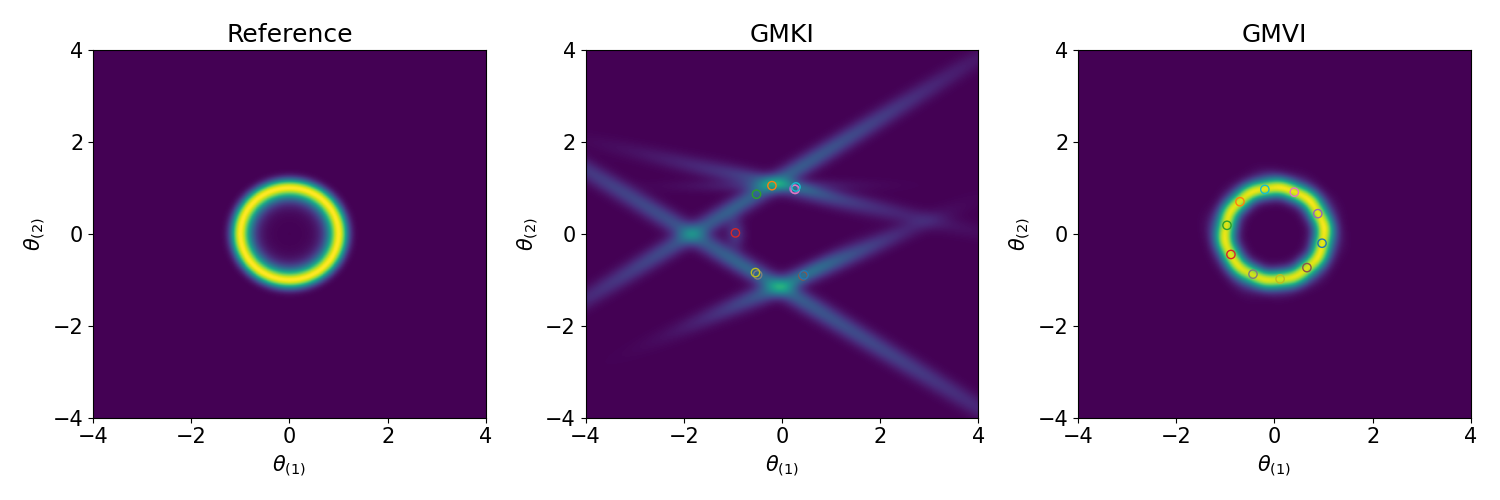
Figure 9: Circle shape posterior: reference posterior distribution (left), posterior distribution obtained by 10-modal GMKI (middle), posterior distribution obtained by 10-modal GMVI (right). Means $m_{k}$ of Gaussian components are marked. In the middle, the color appears lighter because the distribution is concentrated along a thin, elongated line, resulting in a visually diluted effect.

Since the main difference between GMVI Eq. 74 and the continuous time dynamics of GMKI is the derivative-free Kalman approximation for the gradient terms $\nabla_{\theta}\log\rho_{\rm post}$ and $\nabla_{\theta}\nabla_{\theta}\log\rho_{\rm post}$, we understand that the Kalman approximation step leads to the failure of GMKI for sampling the above distribution. It is the goal of future study to investigate other derivative free approximations that can circumvent this failure.

References

References

• [1] Jari Kaipio and Erkki Somersalo. Statistical and computational inverse problems, volume 160. Springer Science & Business Media, 2006.
• [2] Andrew M Stuart. Inverse problems: A Bayesian perspective. Acta numerica, 19:451–559, 2010.
• [3] Steve Brooks, Andrew Gelman, Galin Jones, and Xiao-Li Meng. Handbook of Markov chain Monte Carlo. CRC press, 2011.
• [4] Pierre Del Moral, Arnaud Doucet, and Ajay Jasra. Sequential Monte Carlo samplers. Journal of the Royal Statistical Society: Series B (Statistical Methodology), 68(3):411–436, 2006.
• [5] Nicolas Chopin, Omiros Papaspiliopoulos, et al. An introduction to sequential Monte Carlo, volume 4. Springer, 2020.
• [6] Claudia Tebaldi, Richard L Smith, Doug Nychka, and Linda O Mearns. Quantifying uncertainty in projections of regional climate change: A Bayesian approach to the analysis of multimodel ensembles. Journal of Climate, 18(10):1524–1540, 2005.
• [7] Véronique Gayrard, Anton Bovier, Michael Eckhoff, and Markus Klein. Metastability in reversible diffusion processes i: Sharp asymptotics for capacities and exit times. Journal of the European Mathematical Society, 6(4):399–424, 2004.
• [8] Véronique Gayrard, Anton Bovier, and Markus Klein. Metastability in reversible diffusion processes ii: Precise asymptotics for small eigenvalues. Journal of the European Mathematical Society, 7(1):69–99, 2005.
• [9] Mrinal K Sen and Paul L Stoffa. Global optimization methods in geophysical inversion. Cambridge University Press, 2013.
• [10] Tapio Schneider, Shiwei Lan, Andrew Stuart, and Joao Teixeira. Earth system modeling 2.0: A blueprint for models that learn from observations and targeted high-resolution simulations. Geophysical Research Letters, 44(24):12–396, 2017.
• [11] Charles S Peskin. Numerical analysis of blood flow in the heart. Journal of computational physics, 25(3):220–252, 1977.
• [12] Daniel Z Huang, Dante De Santis, and Charbel Farhat. A family of position-and orientation-independent embedded boundary methods for viscous flow and fluid–structure interaction problems. Journal of Computational Physics, 365:74–104, 2018.
• [13] Daniel Z Huang, Philip Avery, Charbel Farhat, Jason Rabinovitch, Armen Derkevorkian, and Lee D Peterson. Modeling, simulation and validation of supersonic parachute inflation dynamics during Mars landing. In AIAA Scitech 2020 Forum, page 0313, 2020.
• [14] Shunxiang Cao and Daniel Zhengyu Huang. Bayesian calibration for large-scale fluid structure interaction problems under embedded/immersed boundary framework. International Journal for Numerical Methods in Engineering, 2022.
• [15] Marsha J Berger, Phillip Colella, et al. Local adaptive mesh refinement for shock hydrodynamics. Journal of computational Physics, 82(1):64–84, 1989.
• [16] Raunak Borker, Daniel Huang, Sebastian Grimberg, Charbel Farhat, Philip Avery, and Jason Rabinovitch. Mesh adaptation framework for embedded boundary methods for computational fluid dynamics and fluid-structure interaction. International Journal for Numerical Methods in Fluids, 90(8):389–424, 2019.
• [17] Nicolas Moës, John Dolbow, and Ted Belytschko. A finite element method for crack growth without remeshing. International journal for numerical methods in engineering, 46(1):131–150, 1999.
• [18] Zhihong Tan, Colleen M Kaul, Kyle G Pressel, Yair Cohen, Tapio Schneider, and João Teixeira. An extended eddy-diffusivity mass-flux scheme for unified representation of subgrid-scale turbulence and convection. Journal of Advances in Modeling Earth Systems, 10(3):770–800, 2018.
• [19] Ignacio Lopez-Gomez, Costa D Christopoulos, Haakon Ludvig Ervik, Oliver R Dunbar, Yair Cohen, and Tapio Schneider. Training physics-based machine-learning parameterizations with gradient-free ensemble kalman methods. 2022.
• [20] Nicolas Garcia Trillos and Daniel Sanz-Alonso. The Bayesian update: Variational formulations and gradient flows. Bayesian Analysis, 15(1):29–56, 2020.
• [21] N Garcia Trillos, B Hosseini, and D Sanz-Alonso. From optimization to sampling through gradient flows. Notices of the American Mathematical Society, 70(6), 2023.
• [22] Yifan Chen, Daniel Zhengyu Huang, Jiaoyang Huang, Sebastian Reich, and Andrew M Stuart. Sampling via gradient flows in the space of probability measures. arXiv preprint arXiv:2310.03597, 2023.
• [23] Yulong Lu, Jianfeng Lu, and James Nolen. Accelerating langevin sampling with birth-death. arXiv preprint arXiv:1905.09863, 2019.
• [24] Yulong Lu, Dejan Slepčev, and Lihan Wang. Birth-death dynamics for sampling: Global convergence, approximations and their asymptotics. arXiv preprint arXiv:2211.00450, 2022.
• [25] Yifan Chen, Daniel Zhengyu Huang, Jiaoyang Huang, Sebastian Reich, and Andrew M Stuart. Gradient flows for sampling: Mean-field models, Gaussian approximations and affine invariance. arXiv preprint arXiv:2302.11024, 2023.
• [26] Carles Domingo-Enrich and Aram-Alexandre Pooladian. An explicit expansion of the kullback-leibler divergence along its fisher-rao gradient flow. arXiv preprint arXiv:2302.12229, 2023.
• [27] Lezhi Tan and Jianfeng Lu. Accelerate langevin sampling with birth-death process and exploration component. arXiv preprint arXiv:2305.05529, 2023.
• [28] Yifan Chen and Wuchen Li. Optimal transport natural gradient for statistical manifolds with continuous sample space. Information Geometry, 3(1):1–32, 2020.
• [29] Marc Lambert, Sinho Chewi, Francis Bach, Silvère Bonnabel, and Philippe Rigollet. Variational inference via wasserstein gradient flows. arXiv preprint arXiv:2205.15902, 2022.
• [30] Shun-Ichi Amari. Natural gradient works efficiently in learning. Neural computation, 10(2):251–276, 1998.
• [31] James Martens. New insights and perspectives on the natural gradient method. The Journal of Machine Learning Research, 21(1):5776–5851, 2020.
• [32] Guodong Zhang, James Martens, and Roger B Grosse. Fast convergence of natural gradient descent for over-parameterized neural networks. Advances in Neural Information Processing Systems, 32, 2019.
• [33] Wu Lin, Mohammad Emtiyaz Khan, and Mark Schmidt. Fast and simple natural-gradient variational inference with mixture of exponential-family approximations. In International Conference on Machine Learning, pages 3992–4002. PMLR, 2019.
• [34] Yan Chen and Dean S Oliver. Ensemble randomized maximum likelihood method as an iterative ensemble smoother. Mathematical Geosciences, 44(1):1–26, 2012.
• [35] Alexandre A Emerick and Albert C Reynolds. Investigation of the sampling performance of ensemble-based methods with a simple reservoir model. Computational Geosciences, 17(2):325–350, 2013.
• [36] Marco A Iglesias, Kody JH Law, and Andrew M Stuart. Ensemble Kalman methods for inverse problems. Inverse Problems, 29(4):045001, 2013.
• [37] Neil K Chada, Andrew M Stuart, and Xin T Tong. Tikhonov regularization within ensemble Kalman inversion. SIAM Journal on Numerical Analysis, 58(2):1263–1294, 2020.
• [38] Tapio Schneider, Andrew M Stuart, and Jin-Long Wu. Ensemble Kalman inversion for sparse learning of dynamical systems from time-averaged data. arXiv preprint arXiv:2007.06175, 2020.
• [39] Daniel Zhengyu Huang, Tapio Schneider, and Andrew M Stuart. Iterated kalman methodology for inverse problems. Journal of Computational Physics, page 111262, 2022.
• [40] Edoardo Calvello, Sebastian Reich, and Andrew M Stuart. Ensemble Kalman methods: a mean field perspective. arXiv preprint arXiv:2209.11371, 2022.
• [41] Daniel Zhengyu Huang, Jiaoyang Huang, Sebastian Reich, and Andrew M Stuart. Efficient derivative-free Bayesian inference for large-scale inverse problems. Inverse Problems, 38(12):125006, 2022.
• [42] Arnaud Doucet, Adam M Johansen, et al. A tutorial on particle filtering and smoothing: Fifteen years later. Handbook of nonlinear filtering, 12(656-704):3, 2009.
• [43] Michael I Jordan, Zoubin Ghahramani, Tommi S Jaakkola, and Lawrence K Saul. An introduction to variational methods for graphical models. Machine learning, 37(2):183–233, 1999.
• [44] Martin J Wainwright, Michael I Jordan, et al. Graphical models, exponential families, and variational inference. Foundations and Trends® in Machine Learning, 1(1–2):1–305, 2008.
• [45] David M Blei, Alp Kucukelbir, and Jon D McAuliffe. Variational inference: A review for statisticians. Journal of the American statistical Association, 112(518):859–877, 2017.
• [46] Matias Quiroz, David J Nott, and Robert Kohn. Gaussian variational approximation for high-dimensional state space models. arXiv preprint arXiv:1801.07873, 2018.
• [47] Mohammad Khan and Wu Lin. Conjugate-computation variational inference: Converting variational inference in non-conjugate models to inferences in conjugate models. In Artificial Intelligence and Statistics, pages 878–887. PMLR, 2017.
• [48] Théo Galy-Fajou, Valerio Perrone, and Manfred Opper. Flexible and efficient inference with particles for the variational Gaussian approximation. Entropy, 23:990, 2021.
• [49] Caroline Lasser and Christian Lubich. Computing quantum dynamics in the semiclassical regime. Acta Numerica, 29:229–401, 2020.
• [50] William Anderson and Mohammad Farazmand. Fisher information and shape-morphing modes for solving the fokker–planck equation in higher dimensions. Applied Mathematics and Computation, 467:128489, 2024.
• [51] Huan Zhang, Yifan Chen, Eric Vanden-Eijnden, and Benjamin Peherstorfer. Sequential-in-time training of nonlinear parametrizations for solving time-dependent partial differential equations. arXiv preprint arXiv:2404.01145, 2024.
• [52] C Radhakrishna Rao. Information and the accuracy attainable in the estimation of statistical parameters. In Breakthroughs in statistics, pages 235–247. Springer, 1992.
• [53] Nikolai Nikolaevich Cencov. Statistical decision rules and optimal inference. Number 53. American Mathematical Soc., 2000.
• [54] Nihat Ay, Jürgen Jost, Hông Vân Lê, and Lorenz Schwachhöfer. Information geometry and sufficient statistics. Probability Theory and Related Fields, 162(1):327–364, 2015.
• [55] Martin Bauer, Martins Bruveris, and Peter W Michor. Uniqueness of the Fisher–Rao metric on the space of smooth densities. Bulletin of the London Mathematical Society, 48(3):499–506, 2016.
• [56] Yuling Yan, Kaizheng Wang, and Philippe Rigollet. Learning Gaussian mixtures using the wasserstein-fisher-rao gradient flow. arXiv preprint arXiv:2301.01766, 2023.
• [57] Aimee Maurais and Youssef Marzouk. Sampling in unit time with kernel fisher-rao flow. arXiv preprint arXiv:2401.03892, 2024.
• [58] L Wang and N Nüsken. Measure transport with kernel mean embeddings. arXiv preprint arXiv:2401.12967, 2024.
• [59] Oliver G Ernst, Björn Sprungk, and Hans-Jörg Starkloff. Analysis of the ensemble and polynomial chaos Kalman filters in Bayesian inverse problems. SIAM/ASA Journal on Uncertainty Quantification, 3(1):823–851, 2015.
• [60] Alfredo Garbuno-Inigo, Franca Hoffmann, Wuchen Li, and Andrew M Stuart. Interacting Langevin diffusions: Gradient structure and ensemble Kalman sampler. SIAM Journal on Applied Dynamical Systems, 19(1):412–441, 2020.
• [61] Alfredo Garbuno-Inigo, Nikolas Nüsken, and Sebastian Reich. Affine invariant interacting Langevin dynamics for Bayesian inference. SIAM Journal on Applied Dynamical Systems, 19(3):1633–1658, 2020.
• [62] Daniel Alspach and Harold Sorenson. Nonlinear Bayesian estimation using Gaussian sum approximations. IEEE transactions on automatic control, 17(4):439–448, 1972.
• [63] Kazufumi Ito and Kaiqi Xiong. Gaussian filters for nonlinear filtering problems. IEEE transactions on automatic control, 45(5):910–927, 2000.
• [64] Rong Chen and Jun S Liu. Mixture kalman filters. Journal of the Royal Statistical Society: Series B (Statistical Methodology), 62(3):493–508, 2000.
• [65] Sebastian Reich. A Gaussian-mixture ensemble transform filter. Quarterly Journal of the Royal Meteorological Society, 138(662):222–233, 2012.
• [66] Ruoxia Li, Vinay Prasad, and Biao Huang. Gaussian mixture model-based ensemble kalman filtering for state and parameter estimation for a pmma process. Processes, 4(2):9, 2016.
• [67] Rui Fan, Renke Huang, and Ruisheng Diao. Gaussian mixture model-based ensemble kalman filter for machine parameter calibration. IEEE Transactions on Energy Conversion, 33(3):1597–1599, 2018.
• [68] Dario Grana, Torstein Fjeldstad, and Henning Omre. Bayesian Gaussian mixture linear inversion for geophysical inverse problems. Mathematical Geosciences, 49:493–515, 2017.
• [69] Yuming Ba and Lijian Jiang. A residual-driven adaptive Gaussian mixture approximation for Bayesian inverse problems. Journal of Computational and Applied Mathematics, 399:113707, 2022.
• [70] Rudolph Van Der Merwe and Eric Wan. Gaussian mixture sigma-point particle filters for sequential probabilistic inference in dynamic state-space models. In 2003 IEEE International Conference on Acoustics, Speech, and Signal Processing, 2003. Proceedings.(ICASSP’03)., volume 6, pages VI–701. IEEE, 2003.
• [71] Keston W Smith. Cluster ensemble kalman filter. Tellus A: Dynamic Meteorology and Oceanography, 59(5):749–757, 2007.
• [72] Andreas S Stordal, Hans A Karlsen, Geir Nævdal, Hans J Skaug, and Brice Vallès. Bridging the ensemble kalman filter and particle filters: the adaptive Gaussian mixture filter. Computational Geosciences, 15:293–305, 2011.
• [73] Ibrahim Hoteit, Xiaodong Luo, and Dinh-Tuan Pham. Particle Kalman filtering: A nonlinear Bayesian framework for ensemble kalman filters. Monthly weather review, 140(2):528–542, 2012.
• [74] Marco Frei and Hans R Künsch. Mixture ensemble kalman filters. Computational Statistics & Data Analysis, 58:127–138, 2013.
• [75] Thomas Bengtsson, Chris Snyder, and Doug Nychka. Toward a nonlinear ensemble filter for high-dimensional systems. Journal of Geophysical Research: Atmospheres, 108(D24), 2003.
• [76] Alexander Y Sun, Alan P Morris, and Sitakanta Mohanty. Sequential updating of multimodal hydrogeologic parameter fields using localization and clustering techniques. Water Resources Research, 45(7), 2009.
• [77] Andreas S Stordal, Hans A Karlsen, Geir Nævdal, Dean S Oliver, and Hans J Skaug. Filtering with state space localized kalman gain. Physica D: Nonlinear Phenomena, 241(13):1123–1135, 2012.
• [78] José A. Carrillo, Yifan Chen, Daniel Zhengyu Huang, Jiaoyang Huang, and Dongyi Wei. Fisher-rao gradient flow: Geodesic convexity and functional inequality. arXiv preprint, 2024.
• [79] Sebastian Reich. A dynamical systems framework for intermittent data assimilation. BIT Numerical Mathematics, 51(1):235–249, 2011.
• [80] Andrew Gelman and Xiao-Li Meng. Simulating normalizing constants: From importance sampling to bridge sampling to path sampling. Statistical science, pages 163–185, 1998.
• [81] Radford M Neal. Annealed importance sampling. Statistics and computing, 11:125–139, 2001.
• [82] Haoxuan Chen and Lexing Ying. Ensemble-based annealed importance sampling. arXiv preprint arXiv:2401.15645, 2024.
• [83] Nicolas Chopin, Francesca R Crucinio, and Anna Korba. A connection between tempering and entropic mirror descent. arXiv preprint arXiv:2310.11914, 2023.
• [84] Jonathan Goodman and Jonathan Weare. Ensemble samplers with affine invariance. Communications in applied mathematics and computational science, 5(1):65–80, 2010.
• [85] Daniel Foreman-Mackey, David W Hogg, Dustin Lang, and Jonathan Goodman. EMCEE: The MCMC hammer. Publications of the Astronomical Society of the Pacific, 125(925):306, 2013.
• [86] Grigoris A Pavliotis, Andrew M Stuart, and Urbain Vaes. Derivative-free Bayesian inversion using multiscale dynamics. SIAM Journal on Applied Dynamical Systems, 21(1):284–326, 2022.
• [87] Sebastian Reich and Simon Weissmann. Fokker–Planck particle systems for Bayesian inference: Computational approaches. SIAM/ASA Journal on Uncertainty Quantification, 9(2):446–482, 2021.
• [88] Qiang Liu and Dilin Wang. Stein variational gradient descent: A general purpose Bayesian inference algorithm. Advances in neural information processing systems, 29, 2016.