Disentangled Motion Modeling for Video Frame Interpolation

Abstract

Video frame interpolation (VFI) aims to synthesize intermediate frames in between existing frames to enhance visual smoothness and quality. Beyond the conventional methods based on the reconstruction loss, recent works employ the high quality generative models for perceptual quality. However, they require complex training and large computational cost for modeling on the pixel space. In this paper, we introduce disentangled Motion Modeling (MoMo), a diffusion-based approach for VFI that enhances visual quality by focusing on intermediate motion modeling. We propose disentangled two-stage training process, initially training a frame synthesis model to generate frames from input pairs and their optical flows. Subsequently, we propose a motion diffusion model, equipped with our novel diffusion U-Net architecture designed for optical flow, to produce bi-directional flows between frames. This method, by leveraging the simpler low-frequency representation of motions, achieves superior perceptual quality with reduced computational demands compared to generative modeling methods on the pixel space. Our method surpasses state-of-the-art methods in perceptual metrics across various benchmarks, demonstrating its efficacy and efficiency in VFI. Our code is available at: https://github.com/JHLew/MoMo

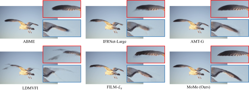
Figure 1: Video Frame Interpolation result of our proposed method (MoMo) with comparison to state-of-the-art methods. Our approach produces the most visually pleasant result, owing to proper modeling of the intermediate motion.

1 Introduction

Video Frame Interpolation (VFI) is a crucial task in computer vision that aims to synthesize absent frames between existing ones in a video. It has a wide spectrum of applications, such as generating slow motion [23], compressing video [68], and producing animation [63]. Its ultimate goal is to elevate the visual quality of videos through enhanced motion smoothness and image sharpness. Motions, represented by optical flows [65, 69, 66, 21] and realized by warping, have been central to VFI’s development as the majority of recent innovations in VFI have been accomplished along with advances in intermediate motion estimation [20, 48, 49, 32, 61, 24, 71, 22, 70, 28, 52, 72, 2, 25, 47, 5].

However, these approaches often result in perceptually unsatisfying outcomes due to their reliance on $L_{1}$ or $L_{2}$ objectives, leading to high PSNR scores but poor perceptual quality [7, 30, 73]. To address this matter, recent advancements [6, 23, 45, 4] have explored the use of deep feature spaces to achieve improved quality in terms of human perception [26, 73]. Additionally, the integration of generative models into VFI [31, 8, 67] has introduced novel pathways for improving the visual quality of videos but has primarily focused on modeling pixels or latent spaces directly, which demands high computational resources.

We introduce disentangled Motion Modeling (MoMo), a perception-oriented approach for VFI, focusing on the modeling of intermediate motions rather than direct pixel generation. We employ a diffusion model [18] to generate bi-directional optical flow maps, marking the first use of generative modeling for motion in VFI. We propose a disentangled two-stage training process that includes the first stage of training a frame synthesis model and fine-tuning of an optical flow estimator [66]. This flow estimator then provides ground-truths in the second stage of training, of our motion diffusion model, which, during inference, generates the motions needed for the synthesis network to create the final interpolated frame. We propose a novel architecture for our motion diffusion model, considering the nature of optical flows, enhancing both computational efficiency and performance.

Our experiments validate the effectiveness and efficiency of our proposed architecture and training scheme, demonstrating superior performance across various benchmarks in terms of perceptual metrics. By focusing on the generative modeling of motions rather than the direct generation of frames, our approach achieves improvements in visual quality, addressing the core objective of VFI.

Our contributions can be summarized as follows:

• We introduce MoMo, a diffusion-based method focusing on generative modeling of bi-directional optical flows for the first time in VFI.

• We propose a two-stage process, disentangling frame synthesis and motion modeling, the two crucial components in VFI.

• We introduce a novel diffusion-model architecture suitable for optical flow modeling, boosting efficiency and quality.

2 Related Work

2.1 Flow-based Video Frame Interpolation

In deep learning-based Video Frame Interpolation (VFI), optical flow-based methods have recently become prominent, and these methods typically follow a common two-stage process. Initially, they estimate the flows needed to create the target intermediate frame, which involves warping of the input frames with these flows. Then, a synthesis network merges the warped images to produce the final frame. The direction of the required flows varies based on the warping technique, either towards or from the target frame. Forward warping, utilized in various studies [45, 44, 25, 24, 20, 43], exploit flows directed towards the target frame. The flows are achieved by linearly adjusting the bi-directional flows between input frames according to the target frame’s intermediate timestep. Conversely, backward warping-based methods focus on estimating flows originating from the target frame, with early approaches also relying on bi-directional flows between input frames [23, 2, 70, 61], which are often converted with flow reversal [70].

Recent advancements in VFI have focused on directly predicting intermediate flows from input frames [22, 28, 35, 72, 32, 48, 49, 47], sparking specialized architectures such as bilateral cost volumes [48, 49, 47] to improve flow accuracy. As VFI quality progresses with flow estimation enhancements, our work aims to improve intermediate flow predictions further. Unlike most methods that rely on reconstruction loss for end-to-end training and some that add flow distillation loss [22, 28, 35, 32] as an auxiliary loss, our approach employs disentangled and direct supervision solely for flow estimation, marking an innovation in VFI research.

2.2 Perception-oriented Restoration

Conventional restoration methods in computer vision, including VFI, focused on minimizing $L_{1}$ or $L_{2}$ distances, often result in blurry images [57, 30, 58, 39] due to prioritizing pixel accuracy over human visual perception. Recent studies have shifted towards deep feature spaces for reconstruction loss [26] and evaluation metrics [73, 10], demonstrating that these align better with human judgment. These approaches emphasize perceptual quality over traditional metrics like PSNR, signaling a move towards more visually appealing, photo-realistic image synthesis.

Moreover, generative models have also been acknowledged for their ability to enhance visual quality in restoration tasks. Early work by Ledig et al. [30] utilized generative adversarial networks (GANs) [16] to produce visually superior restoration results, combining the adversarial loss with traditional reconstruction losses. Beyond GANs, other generative models such as normalizing flows [53, 11, 12] and diffusion models [64, 18] have demonstrated similar observations in improving perceptual quality for restoration tasks [36, 57]. In video frame interpolation (VFI), the adoption of generative models has also been explored [31, 67, 8]. LDMVFI [8], closely related to our work, use latent diffusion models [54] to enhance perceptual quality. Our method aligns with such innovations but uniquely focuses on generating optical flow maps, differing from prior generative approaches that directly model the pixels of the target frame.

2.3 Diffusion Models

Diffusion models [64, 18, 54] are popular generative models that consist of forward and reverse process. Initially, the forward process incrementally adds noise to the data $\textbf{x}_{0}$ over $T$ steps via a predefined Markov chain, resulting in $\textbf{x}_{T}$ that approximates a Gaussian noise. The diffused data $\textbf{x}_{t}$ is obtained through forward process:

$$\textbf{x}_{t}=\sqrt{\alpha_{t}}\textbf{x}_{0}+\sqrt{1-\alpha_{t}}\epsilon,$$ (1)

where $\alpha_{t}\in\{\alpha_{1},...,\alpha_{T}\}$ is a pre-defined noise schedule. Then, the reverse process undoes the forward process by starting from Gaussian noise $\textbf{x}_{T}$ and gradually denoising back to $\textbf{x}_{0}$ over $T$ steps. Diffusion models train a neural network to perform denoising at each step, by minimizing the following objective:

$$L=\mathbb{E}_{\textbf{x}_{0},\epsilon\sim\mathcal{N}(\mathbf{0},\mathbf{I}),t\sim\mathcal{U}(1,T)}\left\|{\epsilon}-{\epsilon}_{\theta}\left({\textbf{x}}_{t},t\right)\right\|_{2}.$$ (2)

While a commonly used approach is to predict the noise as above ($\epsilon$-prediction), there are some alternative approachs, such as $\textbf{x}_{0}$-prediction [51] which predicts the data $\textbf{x}_{0}$ itself or v-prediction [59], which is beneficial for numerical stability.

Diffusion model synthesizes the data in an iterative manner following the backward process, resulting in high perceptual quality of image samples or video samples [9, 56, 19, 17]. Further, we are motivated by optical flow modeling with diffusion models in other tasks [60, 42], and aim to leverage the benefit of diffusion models for optical flow synthesis in video frame interpolation. Although existing work employs diffusion model for video frame interpolation task [8], our method synthesizes the intermediate optical flow rather than directly synthesizing the RGB frames.

3 Method

3.1 Overview

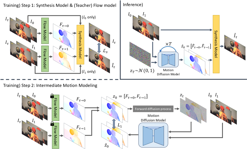
Figure 2: Overview of our entire framework, MoMo. Our framework operates in two stages. Initially, we train a frame synthesis network and an optical flow model, with the latter providing ground-truth labels for the second stage. In the second stage of training, we focus on training a Motion Diffusion Model to predict bi-directional flow between frames. During inference, this model generates flow fields from the input frame pair, enabling the frame synthesis model to output the final target frame.

In this paper, we focus on Video Frame Interpolation (VFI) with the goal of synthesizing an intermediate frame $I_{\tau}$ between consecutive frames $I_{0}$ and $I_{1}$, where $0<\tau<1$. Our method MoMo adopts a two-stage training scheme to disentangle the training of motion modeling and frame synthesis (Fig. 2). In the first stage, we train a frame synthesis network to synthesize an RGB frame from neighboring frames and their bi-directional flows. Then, we fine-tune the optical flow estimator to enhance flow quality. In the second stage, the fine-tuned flow estimator serves as a teacher for training the motion diffusion model. During inference, this model generates intermediate motion, bi-directional flow maps in specific, which the synthesis network uses to produce the final RGB frame.

3.2 Synthesis Network and Teacher Flow Estimator

We propose a synthesis network $\mathcal{S}$, designed to accurately generate an intermediate target frame using a pair of input frames and their corresponding optical flows from the target frames. Specifically, given a frame pair of $I_{0},I_{1}$, and the target intermediate frame $I_{\tau}$, we first use an optical flow network $\mathcal{F}$ to obtain the bi-directional flow from the target frame to the input frames:

$$F_{\tau\rightarrow i}=\mathcal{F}(I_{\tau},I_{i}),i\in\{0,1\},$$ (3)

where $i$ denote the index of input frames. With the estimated flows and their corresponding frames from the target frame, we synthesize $\hat{I}_{\tau}$, which aims to recover the target frame $I_{\tau}$.

$$\hat{I}_{\tau}=\mathcal{S}(I_{in},F_{\tau}),$$ (4)

where $I_{in}$ denotes the input frame pair $\{I_{0},I_{1}\}$ and $F_{\tau}$ denotes the corresponding flow pair $\{F_{\tau\rightarrow 0},F_{\tau\rightarrow 1}\}$.

We adopt pre-trained RAFT [66] for optical flow model $\mathcal{F}$, and train the synthesis network $\mathcal{S}$ from scratch. We choose an alternating optimization of two models, $\mathcal{S}$ and $\mathcal{F}$. We first fix $\mathcal{F}$ to the pre-trained state, and train the synthesis network $\mathcal{S}$. Once the training of $\mathcal{S}$ converges, we freeze it, and fine-tune $\mathcal{F}$. We tune the optical flow model $\mathcal{F}$ so that it could provide better estimations as the teacher in the next stage of training. Note that the flow estimator $\mathcal{F}$ is not used during inference, but serves its purpose as the teacher for intermediate motion modeling described in Sec. 3.3.

Objective

For optimization, we compute loss on the final synthesized output $\hat{I}_{\tau}$, with a combination of three terms. First, we use the pixel reconstruction loss denoted as $\mathcal{L}_{1}$, to minimize the pixel-wise error between the synthesized frame and the target frame: $\mathcal{L}_{1}=||I_{\tau}-\hat{I}_{\tau}||_{1}$. As our ultimate goal is to produce frames of high-quality, we additionally use two losses that are known to be advantageous in promoting perceptual quality, along with $\mathcal{L}_{1}$. Following recent efforts [8, 4], we adopt the LPIPS-based perceptual reconstruction loss [73], denoted as $\mathcal{L}_{p}$, and also exploit the style loss [15] $\mathcal{L}_{G}$, as its effectiveness has been proved in a recent work [52]. By combining the three loss terms, we obtain $\mathcal{L}_{s}$, our perception-oriented reconstruction loss for high quality synthesis:

$$\mathcal{L}_{s}=\lambda_{1}\mathcal{L}_{1}+\lambda_{p}\mathcal{L}_{p}+\lambda_{G}\mathcal{L}_{G}.$$ (5)

Further details on our perception-oriented loss can be found in the Appendix.

3.2.1 Recurrent Synthesis

We build our synthesis network $\mathcal{S}$ to be of recurrent structure, motivated by the recent trend in video frame interpolation [61, 24, 52], due to its great efficiency. Let the number of recurrent process be $L-1$, and $\mathcal{S}$ can be expressed as recurrent application of a synthesis process $\mathcal{P}$:

$$\mathcal{S}(I_{in},F_{\tau})=\mathcal{P}^{0}(\mathcal{P}^{1}(\cdots\mathcal{P}^{L-1}(\hat{I}^{L}_{\tau},I^{L-1}_{in},F^{L-1}_{\tau})\cdots,I^{1}_{in},F^{1}_{\tau}),I^{0}_{in},F^{0}_{\tau}),$$ (6)

where $I_{in}^{l}$ denotes the input image pair $I_{0},I_{1}$ downsampled by a factor of $2^{l}\times$, and $F_{\tau}^{l}$ denotes the flow map pair downsampled likewise.

Our process $\mathcal{P}^{l}$ at level $l$ is described as follows. $\mathcal{P}^{l}$ takes three components as the input: 1) frame $\hat{I}^{l+1}_{\tau}$, synthesized from the previous level $l+1$, 2) downsampled input frame pair $I^{l}_{in}=\{I_{0}^{l},I_{1}^{l}\}$, and 3) the downsampled flow maps $F_{\tau}=\{F_{\tau\rightarrow 0},F_{\tau\rightarrow 1}\}$. First, using the input frame pair $I^{l}_{in}=\{I_{0}^{l},I_{1}^{l}\}$ and its corresponding flow pair $F_{\tau}=\{F_{\tau\rightarrow 0},F_{\tau\rightarrow 1}\}$, we perform backward-warping $(\overleftarrow{\omega})$ on the two frames with their corresponding flows:

$$I^{l}_{\tau\leftarrow i}=\overleftarrow{\omega}(I^{l}_{i},F^{l}_{\tau\rightarrow i}),i\in\{0,1\}.$$ (7)

Next, we take frame $\hat{I}^{l+1}_{\tau}$ and use bicubic upsampling to match the size of level $l$, denoted as $\hat{I}^{l+1\rightarrow l}_{\tau}$. The upsampled frame $\hat{I}^{l+1\rightarrow l}_{\tau}$ and the two warped frames $I^{l}_{\tau\leftarrow 0},I^{l}_{\tau\leftarrow 1}$ are given to the synthesis module $\mathcal{G}$, which outputs a 4 channel output — 1 channel occlusion mask $M_{0}$ to blend $I_{\tau\leftarrow 0}$ and $I_{\tau\leftarrow 1}$, and 3 channel residual RGB values $\Delta\hat{I_{\tau}}$:

$$M^{l}_{0},\Delta\hat{I}^{l}_{\tau}=\mathcal{G}(\hat{I}^{l+1\rightarrow l}_{\tau},I^{l}_{\tau\leftarrow 0},I^{l}_{\tau\leftarrow 1}).$$ (8)

Using these outputs, we obtain the output of $\mathcal{P}^{l}$, the synthesized frame at level $l$:

$$\mathcal{P}^{l}(\hat{I}^{l+1}_{\tau},I_{in}^{l},F_{\tau}^{l})=\hat{I}^{l}_{\tau}=I^{l}_{\tau\leftarrow 0}\odot M^{l}_{0}+I^{l}_{\tau\leftarrow 1}\odot(1-M^{l}_{0})+\Delta\hat{I}^{l}_{\tau}.$$ (9)

Note that $\hat{I}^{L}_{\tau}$ is not available for level $\mathcal{P}^{L-1}$, since it is of the highest level. Therefore we equally blend the two warped frames at level $l=L-1$ as a starting point: $\hat{I}^{L\rightarrow L-1}_{\tau}=I^{L-1}_{\tau\leftarrow 0}\odot 0.5+I^{L-1}_{\tau\leftarrow 1}\odot 0.5$. For our synthesis module $\mathcal{G}$, we use a simple 3-level hierarchy U-Net [55].

3.3 Intermediate Motion Modeling with Diffusion

With a concrete synthesis network prepared, we move on to focus on modeling the intermediate motions for VFI. We use our fine-tuned flow estimator $\mathcal{F}$ as a teacher to train our motion diffusion model $\mathcal{M}$, which generates bi-directional optical flows from given two frames $I_{0}$ and $I_{1}$. Denoting concatenated flows $z_{0}=\{F_{\tau\rightarrow 0},F_{\tau\rightarrow 1}\}$, we train a diffusion model $\mathcal{M}$ by minimizing the following objective:

$$\mathcal{L}_{m}=\mathbb{E}_{z_{0},t\sim\mathcal{U}(1,T)}[||z_{0}-\mathcal{M}(z_{t},t,I_{0},I_{1})||_{1}],$$ (10)

where $z_{t}$ represents noisy flows diffused by Eq. 1. We concatenate $I_{0}$ and $I_{1}$ to $z_{t}$ and keep the teacher $\mathcal{F}$ frozen during training of $\mathcal{M}$. While $\epsilon$-prediction [18] and $L_{2}$ norm are popular choices for training diffusion-based image generative models, we found $x_{0}$-prediction and $L_{1}$ norm to be beneficial for modeling flows. While image diffusion models utilize a U-Net architecture that employs input and output of the same resolution for noisy images that operates fully on the entire resolution, we introduce a new architecture for $\mathcal{M}$ aimed at learning optical flows and enhancing efficiency, which will be described in the following paragraph.

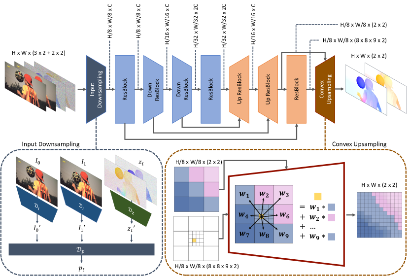
Figure 3: Visualization of our diffusion model architecture. The inputs of two frames and two noisy flow maps, are downsampled and projected respectively, to an $8\times$ smaller resolution. It then goes through a 3-level U-Net, which outputs a pair of coarse flow maps and their corresponding weight masks for upsampling. The convex upsampling layer takes coarse flow maps and the weight masks as the input, and upsamples the coarse flow to the original resolution. Note that the convex upsampling layer accordingly do not have any learnable parameters.

3.3.1 Architecture

In our novel diffusion model architecture designed for motion modeling, we begin by excluding attention layers, as we have found doing so saves memory without deterioration in performance. Observing that optical flow maps—our primary target—are sparse representations encoding only low-frequency information, we opt to avoid the unnecessary complexity of full-resolution flow estimation. Consequently, we predict flows at 1/8 the original resolution, a method mirroring the coarse-to-fine strategies [69, 66, 65, 21], thus sidestepping the need for full-resolution flow estimation. We realize this by introducing input downsampling and convex upsampling, making our architecture computationally efficient and well-suited to meet our resolution-specific needs. We elaborate them in the following paragraphs.

Input Downsampling

Given an input $\{z_{t},~{}I_{0},~{}I_{1}\}$ of 10 channels, we downsample it to $1/8$ size. Rather than using a single layer to directly apply on the 10 channel input, we separately apply different layers on the frames and the noisy flows:

$$I_{0}^{\prime}=\mathcal{D}_{I}(I_{0}),~{}I_{1}^{\prime}=\mathcal{D}_{I}(I_{1}),~{}z_{t}^{\prime}=\mathcal{D}_{z}(z_{t}).$$ (11)

Once we obtain the downsampled features $I_{0}^{\prime},I_{1}^{\prime},z_{t}^{\prime}$, we concatenate and project them to features:

$$p_{t}=\mathcal{D}_{p}([I_{0}^{\prime},I_{1}^{\prime},z_{t}^{\prime}]),$$ (12)

where the projection layer $\mathcal{D}_{p}$ is implemented by a single $1\times 1$ convolutional layer. By sharing the parameters applied to $I_{0}$ and $I_{1}$, we could save the number of parameters required for the downsampling process. In addition, it makes it invariant to the order of taking the two frames.

Convex upsampling

Starting with a coarse flow estimation of size $H/8\times W/8$ from an initial $H\times W$ input, we upsample the predicted flow to the original resolution using a weighted combination of a $3\times 3$ grid from the coarse flow. Utilizing skip connections from the U-Net encoder and a residual block, we generate a mask with $8\times 8\times 9$ channels. Applying softmax to calculate the weights for the 9 neighboring pixels, we then perform a weighted summation to produce the refined flow map. This method aligns with the $\textbf{x}_{0}$-prediction, promoting local correlations and differing from $\epsilon$-predictions which necessitate locally independent estimations.

By operating at a reduced resolution, specifically at $64\times$ smaller space, we achieve significant computation savings. This approach of using diffusion models at a compressed resolution resembles the strategy of latent diffusion models [54], which are noted for their efficiency. Note that this convex upsampling layer does not involve any learnable parameters.

4 Experiments

4.1 Experiment Settings

4.1.1 Implementation Details

We train our model on the Vimeo90k dataset [71], comprising 51,312 triplets designed for VFI, using random $256\times 256$ crops with augmentations like 90^∘ rotation, flipping, and frame order reversing. Since our motion diffusion model is trained on a well-curated data ranging within 256 resolution, it could suffer from a performance drop when it comes to high resolution videos of large motions which goes beyond the distribution of the training data. To handle these cases, we generate flows at the training resolution by resizing the inputs, followed by post-processing of bicubic upsampling at inference time. We recommend the reader to refer to the Appendix for further details.

4.1.2 Evaluation Protocol

We evaluate on well-known VFI benchmarks: SNU-FILM [6], Middlebury (others-set) [1], and Xiph [41, 45], chosen for their broad motion diversity and magnitudes. SNU-FILM is divided into 4 subsets (easy, medium, hard, and extreme) with 310 triplets each, totaling 1240 triplets. The Middlebury benchmark, particularly the others-set, includes 12 frame triplets with a resolution of approximately $640\times 480$. The Xiph benchmark features two subsets, Xiph-2K and Xiph-4K, with 392 frame triplets in 4K resolution. The 2K subset contains 4K triplets downsampled to 2K, while the 4K subset consists of center-cropped 2K patches from the 4K triplets, preserving the original motion magnitudes.

Following practices in generative models-based restoration [8, 33, 46], we use perceptual metrics, LPIPS [73] and DISTS [10] for evaluation. While PSNR and SSIM are popular metrics in evaluating reconstruction quality, they have been known to differ from human perception in some aspects, sensitive to imperceptible differences in pixels and preferring blurry samples [73]. Since our method is based on generative models, we prioritize LPIPS and DISTS, which highly correlates with human perception. The full results including the fidelity metrics such as PSNR and SSIM can be found in the Appendix.

Method	SNU-FILM-easy		SNU-FILM-medium		SNU-FILM-hard		SNU-FILM-extreme
	LPIPS	DISTS	LPIPS	DISTS	LPIPS	DISTS	LPIPS	DISTS
XVFI‡ [61]	0.0251	0.0219	0.0389	0.0304	0.0668	0.0431	0.1189	0.0638
XVFIv [61]	0.0175	0.0181	0.0322	0.0276	0.0629	0.0414	0.1257	0.0673
RIFE [22]	0.0181	0.0195	0.0317	0.0289	0.0657	0.0443	0.1390	0.0764
IFRNet [28]	0.0201	0.0206	0.0320	0.0281	0.0573	0.0398	0.1176	0.0653
FILM-$\mathcal{L}_{1}$ [52]	0.0184	0.0217	0.0315	0.0316	0.0568	0.0441	0.1060	0.0632
ABME [49]	0.0222	0.0229	0.0372	0.0344	0.0658	0.0496	0.1258	0.0747
IFRNet-Large [28]	0.0203	0.0211	0.0321	0.0288	0.0562	0.0403	0.1131	0.0638
UPRNet [24]	0.0179	0.0200	0.0322	0.0311	0.0604	0.0452	0.1115	0.0653
AMT-G [32]	0.0325	0.0312	0.0447	0.0395	0.0680	0.0506	0.1128	0.0686
EMA-VFI [72]	0.0186	0.0204	0.0325	0.0318	0.0579	0.0457	0.1099	0.0671
UPRNet-LARGE [24]	0.0182	0.0203	0.0334	0.0327	0.0612	0.0475	0.1109	0.0672
CAIN† [6]	0.0197	0.0229	0.0375	0.0347	0.0885	0.0606	0.1790	0.1042
FILM-$\mathcal{L}_{vgg}$† [52]	0.0123	0.0128	0.0219	0.0183	0.0443	0.0282	0.0917	0.0471
FILM-$\mathcal{L}_{s}$† [52]	0.0120	0.0124	0.0213	0.0177	0.0429	0.0268	0.0889	0.0448
LDMVFI†‡ [8]	0.0145	0.0130	0.0284	0.0219	0.0602	0.0379	0.1226	0.0651
MoMo† (Ours)	0.0111	0.0102	0.0202	0.0155	0.0419	0.0252	0.0872	0.0433

Table 1: Quantitative experiments on the SNU-FILM benchmark [6]. ${\dagger}$ denotes methods that adopts a perceptual-oriented objective in training. The baseline methods trained without a perceptual-oriented objective are ordered in the ascending order of PSNR scores on the ‘hard’ subset, from lower scoring ones located on top, and higher scoring ones at the bottom. ${\ddagger}$ denotes that the method used different / additional data in training. The best results are in bold, and the second best is underlined, respectively.

Method	Middlebury		Xiph-2K		Xiph-4K
	LPIPS	DISTS	LPIPS	DISTS	LPIPS	DISTS
XVFI‡ [61]	0.0520	0.0557	0.0710	0.0360	0.1222	0.0610
XVFIv [61]	0.0169	0.0244	0.0844	0.0418	0.1835	0.0779
RIFE [22]	0.0162	0.0228	0.0918	0.0481	0.2072	0.0915
FILM-$\mathcal{L}_{1}$ [52]	0.0173	0.0246	0.0906	0.0510	0.1841	0.0884
ABME [49]	0.0290	0.0325	0.1071	0.0581	0.2361	0.1108
IFRNet-Large [28]	0.0285	0.0366	0.0681	0.0372	0.1364	0.0665
AMT-G [32]	0.0486	0.0533	0.1061	0.0563	0.2054	0.1005
EMA-VFI [72]	0.0151	0.0218	0.1024	0.0550	0.2258	0.1049
UPRNet-LARGE [24]	0.0150	0.0209	0.1010	0.0553	0.2150	0.1017
CAIN† [6]	0.0254	0.0383	0.1025	0.0533	0.2229	0.0980
FILM-${\mathcal{L}_{vgg}}^{{\dagger}}$ [52]	0.0096	0.0148	0.0355	0.0238	0.0754	0.0406
FILM-$\mathcal{L}_{s}$† [52]	0.0093	0.0140	0.0330	0.0237	0.0703	0.0385
LDMVFI†‡ [8]	0.0195	0.0261	0.0420	0.0163	0.0859	0.0359
MoMo† (Ours)	0.0094	0.0126	0.0300	0.0119	0.0631	0.0274

Table 2: Quantitative experiments on the three benchmarks, Middlebury [1], and Xiph-2K and Xiph-4K [41, 45]. ${\dagger}$ denotes methods that adopts a perceptual-oriented objective in training. The baseline methods trained without a perceptual-oriented objective are ordered in the PSNR scores on the ‘hard’ subset, from lower scoring ones on the top, to higher scoring ones towards the bottom. ${\ddagger}$ denotes that the method used different / additional data in training. The best results are in bold, and the second best is underlined, respectively.

4.2 Comparison to State-of-the-arts

To validate the effectiveness of our approach, we compare MoMo with state-of-the-art VFI methods. The methods for comparison include: CAIN [6], FILM-$\mathcal{L}_{vgg}$, FILM-$\mathcal{L}_{s}$ and LDMVFI [8], which employ with perceptual-oriented loss in the training process. Since models trained for improved perceptual quality are publicly available by a very limited number, we also include methods trained with the traditional pixel-wise reconstruction loss: XVFI [61], RIFE [22], IFRNet [28], FILM-$\mathcal{L}_{1}$ [52], ABME [49], UPRNet [24], AMT [32], EMA-VFI [72].

4.2.1 Quantitative Results

Tables 1 and 2 present our quantitative results across three benchmark datasets. We order the baseline methods which rely on the traditional pixel-wise reconstruction loss by their PSNR scores on SNU-FILM’s ‘hard’ subset, with lower and higher PSNR scores at the top and bottom, respectively. This order suggests PSNR may not always reflect human perception, with higher PSNR models exhibiting lower perceptual quality at times.

MoMo achieves state-of-the-art on all SNU-FILM subsets, leading in both LPIPS and DISTS metrics. On Middlebury, it outperforms baselines in DISTS and closely trails FILM-$\mathcal{L}_{s}$ in LPIPS. MoMo also excels on both Xiph subsets, 2K and 4K, in both metrics. MoMo surpasses methods like XVFI, FILM, and UPRNet, tailored for high-resolution flow estimation. This highlights the effectiveness of our approach in generating well-structured optical flows for the intermediate frame through proficient intermediate motion modeling.

To support our discussion, we provide a visualization of flow estimations and the frame synthesis outcomes, with comparison to state-of-the-art algorithms at Fig. 4. Although XVFI and FILM takes advantage of the recurrent architecture tailored for flow estimations at high resolution images, they fail in well-structured flow estimations and frame synthesis. XVFI largely fails in flow estimation, which results in blurry outputs. The estimations by FILM display vague and noisy motion boundaries, especially in $F_{\tau\rightarrow 1}$. Another important point to note is that the flow pair $F_{\tau\rightarrow 0}$ and $F_{\tau\rightarrow 1}$ of FILM do not align well with each other, causing confusion in the synthesis process.

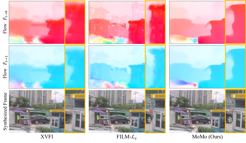
Figure 4: Visualized comparison of estimated intermediate flows against state-of-the-art methods. Although XVFI [61] and FILM [52] is designed for estimating of elaborate flows on high resolution images, it sometimes fails to predict well-structured flow fields, leading to unpleasant synthesis results. On the other hand, our flow estimations consistently show a well-structured flow fields which leads to promising synthesis of frames.

4.2.2 Qualitative Results

The qualitative results of MoMo with comparison to the state-of-the-art algorithms can be found at Fig. 1 and 5. In Fig. 1, it can be found that MoMo reconstructs both wings with rich details, whereas methods of the top row, which greatly relies on the $L_{1}$ pixel-wise loss in training, namely ABME [49], IFRNet [28] and AMT [32] all show blurry results. Moreover, our result also outperforms state-of-the-art models designed particularly for perceptual quality, LDMVFI [8] and FILM-$\mathcal{L}_{s}$ [52], with well-structurized synthesis of both wings. Fig. 5 present additional results obtained from the ‘extreme’ subset of SNU-FILM and Xiph-4K set. Here, we compare with LDMVFI [8] and FILM-$\mathcal{L}_{s}$ [52], methods designed specifically for visual quality, along with FILM-$\mathcal{L}_{1}$ [52]. We use FILM-$\mathcal{L}_{1}$ [52] as a representative among the $L_{1}$ reconstruction-based method, as it performed the most robust and competently in terms of perceptual metrics across multiple benchmarks as reported in Tab. 1 and 2. MoMo consistently shows a superior visual quality, with less artifacts and well-structured objects.

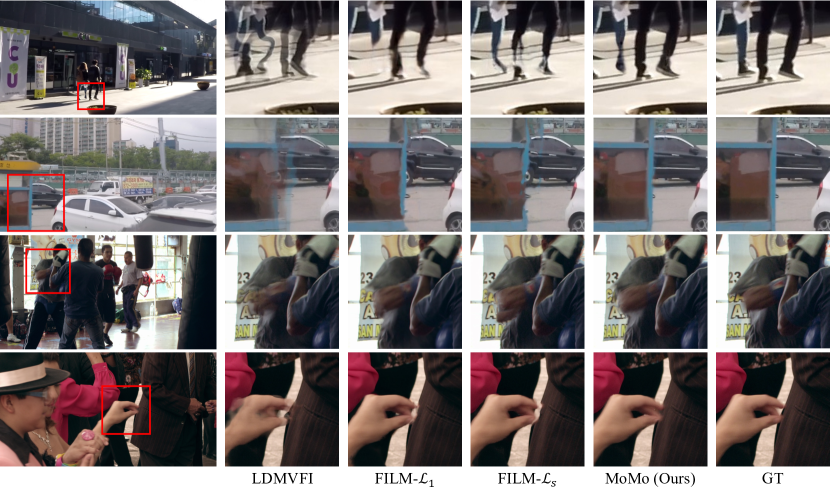
Figure 5: Qualitative comparison against state-of-the-art methods on ‘extreme’ subset of SNU-FILM and Xiph-4K. Our results show the least artifacts and generate well-structured images.

4.3 Ablation Studies

To verify the effects of our design choices, the ablation studies in the following sections are conducted on the ‘hard’ subset of SNU-FILM dataset, unless mentioned otherwise. We start by studying the effects of the teacher optical flow model, used for training the motion diffusion model. We then experiment on the number of denoising steps used at inference time. Last but not least, we study on the design choices in diffusion architecture, namely the use of $\textbf{x}_{0}$-prediction and our U-Net with convex upsampling.

Teacher	LPIPS	DISTS
Pre-trained	0.0445	0.0284
End-to-End	0.0475	0.0287
Fine-tuned (proposed)	0.0419	0.0252

Table 3: Ablation on the teacher flow model. We use the RAFT [66] model fixed to the pre-trained state, fine-tuned after training the synthesis model, and trained with the synthesis model in an end-to-end manner. Our experiments show that fine-tuning after training the synthesis model is the most effective.

# of steps	LPIPS	DISTS
1 step ($\approx$ non-diffusion)	0.0892	0.0452
8 step (default)	0.0872	0.0433
20 step	0.0872	0.0433
50 step	0.0874	0.0435

Table 4: Experiment on the number of denoising steps for inference (on SNU-FILM-extreme). Our experiments show that about 8 steps is enough, and use of more steps exceeding this does not lead to a notable improvement considering the runtime tradeoff.

4.3.1 Optical Flow Teacher

We conduct ablation study on the teacher optical flow model. We choose RAFT [66] as the teacher model, which is the state-of-the-art architecture for optical flow estimation. We prepare the teacher model of three different weights. 1) we use the default off-the-shelf weights provided by the Torchvision library [37],trained specifically for optical flow estimation on multiple datasets [13, 38, 3, 40, 27]. 2) we fine-tune the pre-trained RAFT with our frozen synthesis model as described in Sec. 3.2. 3) we jointly train RAFT and our synthesis network in end-to-end manner, with RAFT initialized with the pre-trained weights. We use these three RAFT models of different weights as the teacher for the experiment.

The ablation study summarized in Table 4 shows that fine-tuning the flow model $\mathcal{F}$ after training the synthesis model $\mathcal{G}$ is the most effective, while concurrent training is the least effective. Fine-tuning of $\mathcal{F}$ enhances flow estimation and suitability for synthesis tasks [71]. However, end-to-end training can cause the synthesis model to depend too heavily on estimated flows, risking inaccuracies from the motion diffusion model. Our results highlight that sequential training of the synthesis model and the flow estimator ensures optimal performance.

4.3.2 Number of Steps

Table 4 shows the effect of number of denoising steps in motion generation, experimented on the ‘extreme’ subset of SNU-FILM. We find that around 8 steps is optimal, with more steps not markedly improving performance. This is likely due to the simpler nature of flow representations compared to RGB pixels. In contrast to image diffusion models [54] and LDMVFI [8] which requires over 50 steps, our method delivers satisfactory outcomes with far fewer steps, cutting down on both runtime and computational expenses.

4.3.3 Diffusion Architecture

Data	Prediction	Architecture	LPIPS	DISTS	FLOPs (T)	Params. (M)	Runtime (ms)
Latent	$\epsilon$	Standard U-Net [8]	0.0601	0.0379	3.25	439.0	10283.51
Flow	$\epsilon$	Standard U-Net	0.4090	0.2621	8.08	69.1	603.64
Flow	$\textbf{x}_{0}$	Standard U-Net	0.0460	0.0295	8.08	69.1	603.64
Flow	$\textbf{x}_{0}$ (weighted)	Convex-Up U-Net (Ours)	0.0463	0.0298	1.12	71.6	145.49
Flow	$\textbf{x}_{0}$	Convex-Up U-Net (Ours)	0.0419	0.0252	1.12	71.6	145.49

Table 5: We conduct an ablation study on our diffusion model, emphasizing its minimal computational needs and fastest runtime. The results showcase the entire framework’s performance, covering both diffusion and synthesis stages. For reference, the first row includes LDMVFI’s approach, which relies on a larger diffusion model and a vector-quantized [14] decoder, leading to a notably slower runtime than ours.

In our ablation study, detailed in Table 5, we assess our motion diffusion model using the standard timestep-conditioned U-Net architecture (UNet2DModel) from the diffusers library [50], alongside $\epsilon$- and $\textbf{x}_{0}$-prediction types. Contrary to the common preference for $\epsilon$-prediction in diffusion models, our motion diffusion model favors $\textbf{x}_{0}$-prediction.

We also explore our coarse-to-fine estimation using convex upsampling [66]. This approach reduces computational costs by operating at a lower resolution and improves performance. Given that our architecture predicts values with a strong correlation between neighboring pixels, $\epsilon$-prediction, which samples noise independently, proves less suitable. We experiment with a SNR-weighted $\textbf{x}_{0}$-prediction [59], to make it equivalent to $\epsilon$-prediction loss. Nonetheless, $\textbf{x}_{0}$-prediction consistently outperforms, validating our architectural decisions.

Despite having a similar number of parameters as the standard U-Net, our Convex Upsampling U-Net significantly reduces floating point operations (FLOPs) by about $7.2\times$. Runtime tests on a NVIDIA 32GB V100 GPU for $256\times 448$ resolution frames—averaged over 100 iterations—reveal that our Convex-Up U-Net processes frames in approximately 145.49 ms each, achieving a $4.15\times$ speedup over the standard U-Net and an $70\times$ faster inference speed than the LDMVFI [8] baseline. This efficiency is attributed to our model’s efficient architecture and notably fewer denoising steps.

5 Limitation and Future Work

As mentioned in Sec. 4.1.1, our framework generates flows at a resized resolution, followed by bicubic upsampling during inference. Consequently, the generated flows could lack in details at motion boundaries, although it still performs superior to baseline methods. By adopting an recurrent architecture for the motion diffusion model, as in recent efforts in large motion estimation [61, 52, 24], we believe our approach could be further reinforced, and leave this for future work.

6 Conclusion

In this paper, we proposed MoMo, a disentangled motion modeling framework for perceptual video frame interpolation. Our approach mainly focuses on modeling the intermediate motions between frames, with explicit supervision on the motions. We introduced motion diffusion model, which generates intermediate bi-directional flows necessary to synthesize the target frame. We also presented a novel architecture for diffusion models, tailored for optical flow generation, which greatly improves both performance and computational efficiency. Extensive experiments confirm that our method achieve state-of-the-art quality on multiple benchmarks.

6.0.1 Acknowledgement

This work was partly supported by Institute of Information & communications Technology Planning & Evaluation (IITP) grant funded by the Korea government(MSIT) [NO.RS-2021-II211343, Artificial Intelligence Graduate School Program (Seoul National University)], the National Research Foundation of Korea (NRF) grant funded by the Korea government (MSIT) (No. 2022R1A3B1077720) and the BK21 FOUR program of the Education and the Research Program for Future ICT Pioneers, Seoul National University in 2024.

Appendix 0.A Implementation Details

0.A.1 Perception-oriented loss

As mentioned in Sec. 3.2, we specify the objective function we use for stage 1 training. Along with the $L_{1}$ pixel reconstruction loss, we use an LPIPS-based perceptual loss, which computes the $L_{2}$ distance in the deep feature space of AlexNet [29]. This loss is well-known for high correlation with human judgements. Next, we exploit the style loss [15] $\mathcal{L}_{G}$ as its effectiveness has been proved in a recent work [52]. This loss computes the $L_{2}$ distance of feature correlations extracted from the VGG-19 network [62]:

$$\mathcal{L}_{G}=\frac{1}{N}\sum^{N}_{n=1}\alpha_{n}||G_{n}(I_{\tau})-G_{n}(\hat{I}_{\tau})||_{2}.$$ (13)

Here, $\alpha_{n}$ denotes the weighting hyper-parameter of the $n$-th selected layer. Denoting the feature map of frame $I_{\tau}$ extracted from $n$-th selected layer of the VGG [62] network as $\phi_{n}(I_{\tau})\in\mathbb{R}^{H\times W\times C}$, the Gram matrix of frame $I_{\tau}$ at the $n$-th feature space, $G_{n}(I_{\tau})\in\mathbb{R}^{C\times C}$ can be acquired as follows:

$$G_{n}(I_{\tau})=\phi_{n}(I_{\tau})^{\top}\phi_{n}(I_{\tau}).$$ (14)

Likewise, the Gram matrix of our synthesized frame, $G_{n}(\hat{I}_{\tau})$, could be computed by substituting $I_{\tau}$ with $\hat{I}_{\tau}$ in Eq. 14.

0.A.2 Training Details

We elaborate on our training parameters as mentioned in Sec 4.1.

Stage 1 Training

We employ the AdamW optimizer [34], setting the weight decay to $10^{-4}$ and the batch size to 32 both in the training process of $\mathcal{G}$ and $\mathcal{F}$. We train the synthesis model $\mathcal{G}$ for a total of 200 epochs, with a fixed learning rate of $2\times 10^{-4}$. For the first 150 epochs, we set the hyper-parameters to $\lambda_{1}=1,\lambda_{p}=0,\lambda_{G}=0$. After that, we use $\lambda_{1}=1,\lambda_{p}=1,\lambda_{G}=20$ for the last 50 epochs. Once the synthesis model is fully trained, we fine-tune the teacher flow model $\mathcal{F}$ for 100 epochs, with its learning rate fixed to $10^{-4}$. We set hyper-parameters to $\lambda_{1}=1,\lambda_{p}=1,\lambda_{G}=20$. Both $\mathcal{G}$ and $\mathcal{F}$ benefit from an exponential moving average (EMA) with a 0.999 decay rate. We set the number of pyramids $L=3$ during training, and use $L=\lceil\log_{2}(R/32)\rceil$ for resolution $R$ at inference.

Stage 2 Training

We train our diffusion model for 500 epochs using the AdamW optimizer with a constant learning rate of $2\times 10^{-4}$, weight decay of $10^{-8}$, and batch size of 64, applying an EMA with a 0.9999 decay rate. Given that diffusion models typically operate with data values between $[-1,1]$ but optical flows often exceed this range, we normalize flow values by dividing them by 128. This adjustment ensures flow values to be compatible with the diffusion model’s expected data range, effectively aligning flow values with those of the RGB space, which are similarly normalized. We utilize a linear noise schedule [18] and perform 8 denoising steps using the ancestral DDPM sampler [18] for efficient sampling.

Appendix 0.B Additional Results

0.B.1 Deeper Analysis on Number of Denoising Steps

We experiment on the effect of different number of denoising steps for motion modeling, on the ‘hard’ subset of SNU-FILM.(Tab.6) Although the performance does improve up to 8 steps, the increase is relatively marginal compared to the results on the ‘extreme’ subset. We speculate the reason for this result is due to the smaller ill-posedness of the ‘hard’ subset, which limits the diversity of feasible flows. We claim that the use of more steps and the design choice of diffusion models for motion modeling gets more advantageous as the ill-posedness of motions gets larger.

# of steps	SNU-FILM-hard		SNU-FILM-extreme
	LPIPS	DISTS	LPIPS	DISTS
1 step	0.0421	0.0254	0.0892	0.0452
8 step (default)	0.0419	0.0252	0.0872	0.0433
20 step	0.0420	0.0253	0.0872	0.0433
50 step	0.0420	0.0254	0.0874	0.0435

Table 6: Experiment on the number of denoising steps at inference time. Our experiments show that about 8 steps is enough, and use of more steps exceeding this does not lead to a notable improvement considering the runtime tradeoff.

0.B.2 Full Quantitative Results

We report the full quantitative results including the fidelity metrics such as PSNR and SSIM on the SNU-FILM (Tab. 7, 8), Middlebury (Tab. 9) and Xiph benchmarks (Tab. 10).

Method	SNU-FILM-easy				SNU-FILM-medium
	PSNR	SSIM	LPIPS	DISTS	PSNR	SSIM	LPIPS	DISTS
XVFI‡ [61]	38.57	0.9824	0.0251	0.0219	34.56	0.9635	0.0389	0.0304
XVFIv [61]	39.78	0.9865	0.0175	0.0181	35.36	0.9692	0.0322	0.0276
RIFE [22]	40.06	0.9907	0.0181	0.0195	35.75	0.9789	0.0317	0.0289
IFRNet [28]	40.03	0.9905	0.0201	0.0206	35.94	0.9793	0.0320	0.0281
FILM-$\mathcal{L}_{1}$ [52]	39.74	0.9902	0.0184	0.0217	35.81	0.9789	0.0315	0.0316
ABME [49]	39.59	0.9901	0.0222	0.0229	35.77	0.9789	0.0372	0.0344
IFRNet-Large [28]	40.10	0.9906	0.0203	0.0211	36.12	0.9797	0.0321	0.0288
UPRNet [24]	40.37	0.9910	0.0179	0.0200	36.16	0.9797	0.0322	0.0311
AMT-G [32]	38.47	0.9880	0.0325	0.0312	35.39	0.9779	0.0447	0.0395
EMA-VFI [72]	39.52	0.9903	0.0186	0.0204	35.83	0.9795	0.0325	0.0318
UPRNet-LARGE [24]	40.44	0.9911	0.0182	0.0203	36.29	0.9801	0.0334	0.0327
CAIN† [6]	39.89	0.9900	0.0197	0.0229	35.61	0.9776	0.0375	0.0347
FILM-$\mathcal{L}_{vgg}$† [52]	39.79	0.9900	0.0123	0.0128	35.77	0.9782	0.0219	0.0183
FILM-$\mathcal{L}_{s}$† [52]	39.68	0.9900	0.0120	0.0124	35.70	0.9781	0.0213	0.0177
LDMVFI†‡ [8]	38.68	0.9834	0.0145	0.0130	33.90	0.9703	0.0284	0.0219
MoMo† (Ours)	39.64	0.9895	0.0111	0.0102	35.45	0.9769	0.0202	0.0155

Table 7: Full quantitative results including the fidelity metrics (PSNR, SSIM) on the ‘easy’ and ‘medium’ subsets of SNU-FILM benchmark [6]. ${\dagger}$ denotes methods that adopts a perceptual-oriented objective in training. The baseline methods trained without a perceptual-oriented objective are ordered in the ascending order of PSNR scores on the ‘hard’ subset, from lower scoring ones located on top, and higher scoring ones at the bottom. ${\ddagger}$ denotes that the method used different / additional data in training. The best results are in bold, and the second best is underlined, respectively.

Method	SNU-FILM-hard				SNU-FILM-extreme
	PSNR	SSIM	LPIPS	DISTS	PSNR	SSIM	LPIPS	DISTS
XVFI‡ [61]	29.56	0.9028	0.0668	0.0431	24.89	0.8095	0.1189	0.0638
XVFIv [61]	29.91	0.9073	0.0629	0.0414	24.67	0.8092	0.1257	0.0673
RIFE [22]	30.10	0.9330	0.0657	0.0443	24.84	0.8534	0.1390	0.0764
IFRNet [28]	30.41	0.9358	0.0573	0.0398	25.05	0.8587	0.1176	0.0653
FILM-$\mathcal{L}_{1}$ [52]	30.42	0.9353	0.0568	0.0441	25.17	0.8593	0.1060	0.0632
ABME [49]	30.58	0.9364	0.0658	0.0496	25.42	0.8639	0.1258	0.0747
IFRNet-Large [28]	30.63	0.9368	0.0562	0.0403	25.27	0.8609	0.1131	0.0638
UPRNet [24]	30.67	0.9365	0.0604	0.0452	25.49	0.8627	0.1115	0.0653
AMT-G [32]	30.70	0.9381	0.0680	0.0506	25.64	0.8658	0.1128	0.0686
EMA-VFI [72]	30.79	0.9386	0.0579	0.0457	25.59	0.8648	0.1099	0.0671
UPRNet-LARGE [24]	30.86	0.9377	0.0612	0.0475	25.63	0.8641	0.1109	0.0672
CAIN† [6]	29.90	0.9292	0.0885	0.0606	24.78	0.8507	0.1790	0.1042
FILM-$\mathcal{L}_{vgg}$† [52]	30.34	0.9332	0.0443	0.0282	25.11	0.8557	0.0917	0.0471
FILM-$\mathcal{L}_{s}$† [52]	30.29	0.9329	0.0429	0.0268	25.07	0.8550	0.0889	0.0448
LDMVFI†‡ [8]	28.51	0.9173	0.0602	0.0379	23.92	0.8372	0.1226	0.0651
MoMo† (Ours)	30.12	0.9312	0.0419	0.0252	25.02	0.8547	0.0872	0.0433

Table 8: Full quantitative results including the fidelity metrics (PSNR, SSIM) on the ‘hard’ and ‘extreme’ subsets of SNU-FILM benchmark [6]. ${\dagger}$ denotes methods that adopts a perceptual-oriented objective in training. The baseline methods trained without a perceptual-oriented objective are ordered in the ascending order of PSNR scores on the ‘hard’ subset, from lower scoring ones located on top, and higher scoring ones at the bottom. ${\ddagger}$ denotes that the method used different / additional data in training. The best results are in bold, and the second best is underlined, respectively.

Method	Middlebury
	PSNR	SSIM	LPIPS	DISTS
XVFI‡ [61]	33.43	0.9557	0.0520	0.0557
XVFIv [61]	36.72	0.9826	0.0169	0.0244
RIFE [22]	37.16	0.9853	0.0162	0.0228
FILM-$\mathcal{L}_{1}$ [52]	37.37	0.9838	0.0173	0.0246
ABME [49]	37.05	0.9845	0.0290	0.0325
IFRNet-Large [28]	36.27	0.9816	0.0285	0.0366
AMT-G [32]	34.23	0.9708	0.0486	0.0533
EMA-VFI [72]	38.32	0.9871	0.0151	0.0218
UPRNet-LARGE [24]	38.09	0.9861	0.0150	0.0209
CAIN† [6]	35.11	0.9761	0.0254	0.0383
FILM-${\mathcal{L}_{vgg}}^{{\dagger}}$ [52]	37.28	0.9843	0.0096	0.0148
FILM-$\mathcal{L}_{s}$† [52]	37.38	0.9844	0.0093	0.0140
LDMVFI†‡ [8]	34.03	0.9648	0.0195	0.0261
MoMo† (Ours)	36.77	0.9806	0.0094	0.0126

Table 9: Full quantitative results including the fidelity metrics (PSNR, SSIM) on Middlebury [1] benchmark. ${\dagger}$ denotes methods that adopts a perceptual-oriented objective in training. The baseline methods trained without a perceptual-oriented objective are ordered in the PSNR scores on the ‘hard’ subset, from lower scoring ones on the top, to higher scoring ones towards the bottom. ${\ddagger}$ denotes that the method used different / additional data in training. The best results are in bold, and the second best is underlined, respectively.

Method	Xiph-2K				Xiph-4K
	PSNR	SSIM	LPIPS	DISTS	PSNR	SSIM	LPIPS	DISTS
XVFI‡ [61]	34.75	0.9560	0.0710	0.0360	32.83	0.9231	0.1222	0.0610
XVFIv [61]	35.17	0.9625	0.0844	0.0418	32.45	0.9274	0.1835	0.0779
RIFE [22]	36.06	0.9642	0.0918	0.0481	33.21	0.9413	0.2072	0.0915
FILM-$\mathcal{L}_{1}$ [52]	36.53	0.9663	0.0906	0.0510	33.83	0.9439	0.1841	0.0884
ABME [49]	36.50	0.9668	0.1071	0.0581	33.72	0.9452	0.2361	0.1108
IFRNet-Large [28]	36.40	0.9646	0.0681	0.0372	33.71	0.9425	0.1364	0.0665
AMT-G [32]	36.29	0.9647	0.1061	0.0563	34.55	0.9472	0.2054	0.1005
EMA-VFI [72]	36.74	0.9675	0.1024	0.0550	34.55	0.9486	0.2258	0.1049
UPRNet-LARGE [24]	37.13	0.9691	0.1010	0.0553	34.57	0.9388	0.2150	0.1017
CAIN† [6]	35.18	0.9625	0.1025	0.0533	32.55	0.9398	0.2229	0.0980
FILM-${\mathcal{L}_{vgg}}^{{\dagger}}$ [52]	36.29	0.9626	0.0355	0.0238	33.44	0.9356	0.0754	0.0406
FILM-$\mathcal{L}_{s}$† [52]	36.30	0.9616	0.0330	0.0237	33.37	0.9323	0.0703	0.0385
LDMVFI†‡ [8]	33.82	0.9494	0.0420	0.0163	31.39	0.9214	0.0859	0.0359
MoMo† (Ours)	35.38	0.9553	0.0300	0.0119	33.09	0.9293	0.0631	0.0274

Table 10: Full quantitative results including the fidelity metrics (PSNR, SSIM) on Xiph-2K and Xiph-4K [41, 45]. ${\dagger}$ denotes methods that adopts a perceptual-oriented objective in training. The baseline methods trained without a perceptual-oriented objective are ordered in the PSNR scores on the ‘hard’ subset, from lower scoring ones on the top, to higher scoring ones towards the bottom. ${\ddagger}$ denotes that the method used different / additional data in training. The best results are in bold, and the second best is underlined, respectively.

References

- [1] Baker, S., Scharstein, D., Lewis, J., Roth, S., Black, M.J., Szeliski, R.: A database and evaluation methodology for optical flow. International journal of computer vision 92, 1–31 (2011)
- [2] Bao, W., Lai, W.S., Ma, C., Zhang, X., Gao, Z., Yang, M.H.: Depth-aware video frame interpolation. In: Proceedings of the IEEE/CVF conference on computer vision and pattern recognition. pp. 3703–3712 (2019)
- [3] Butler, D.J., Wulff, J., Stanley, G.B., Black, M.J.: A naturalistic open source movie for optical flow evaluation. In: Computer Vision–ECCV 2012: 12th European Conference on Computer Vision, Florence, Italy, October 7-13, 2012, Proceedings, Part VI 12. pp. 611–625. Springer (2012)
- [4] Chen, S., Zwicker, M.: Improving the perceptual quality of 2d animation interpolation. In: European Conference on Computer Vision. pp. 271–287. Springer (2022)
- [5] Chi, Z., Mohammadi Nasiri, R., Liu, Z., Lu, J., Tang, J., Plataniotis, K.N.: All at once: Temporally adaptive multi-frame interpolation with advanced motion modeling. In: Computer Vision–ECCV 2020: 16th European Conference, Glasgow, UK, August 23–28, 2020, Proceedings, Part XXVII 16. pp. 107–123. Springer (2020)
- [6] Choi, M., Kim, H., Han, B., Xu, N., Lee, K.M.: Channel attention is all you need for video frame interpolation. In: AAAI (2020)
- [7] Danier, D., Zhang, F., Bull, D.: A subjective quality study for video frame interpolation. In: 2022 IEEE International Conference on Image Processing (ICIP). pp. 1361–1365. IEEE (2022)
- [8] Danier, D., Zhang, F., Bull, D.: Ldmvfi: Video frame interpolation with latent diffusion models. arXiv preprint arXiv:2303.09508 (2023)
- [9] Dhariwal, P., Nichol, A.: Diffusion models beat gans on image synthesis. Advances in neural information processing systems 34, 8780–8794 (2021)
- [10] Ding, K., Ma, K., Wang, S., Simoncelli, E.P.: Image quality assessment: Unifying structure and texture similarity. CoRR abs/2004.07728 (2020), https://arxiv.org/abs/2004.07728
- [11] Dinh, L., Krueger, D., Bengio, Y.: Nice: Non-linear independent components estimation. arXiv preprint arXiv:1410.8516 (2014)
- [12] Dinh, L., Sohl-Dickstein, J., Bengio, S.: Density estimation using real nvp. arXiv preprint arXiv:1605.08803 (2016)
- [13] Dosovitskiy, A., Fischer, P., Ilg, E., Hausser, P., Hazirbas, C., Golkov, V., Van Der Smagt, P., Cremers, D., Brox, T.: Flownet: Learning optical flow with convolutional networks. In: Proceedings of the IEEE international conference on computer vision. pp. 2758–2766 (2015)
- [14] Esser, P., Rombach, R., Ommer, B.: Taming transformers for high-resolution image synthesis. In: Proceedings of the IEEE/CVF conference on computer vision and pattern recognition. pp. 12873–12883 (2021)
- [15] Gatys, L.A., Ecker, A.S., Bethge, M.: Image style transfer using convolutional neural networks. In: Proceedings of the IEEE conference on computer vision and pattern recognition. pp. 2414–2423 (2016)
- [16] Goodfellow, I., Pouget-Abadie, J., Mirza, M., Xu, B., Warde-Farley, D., Ozair, S., Courville, A., Bengio, Y.: Generative adversarial nets. Advances in neural information processing systems 27 (2014)
- [17] Ho, J., Chan, W., Saharia, C., Whang, J., Gao, R., Gritsenko, A., Kingma, D.P., Poole, B., Norouzi, M., Fleet, D.J., et al.: Imagen video: High definition video generation with diffusion models. arXiv preprint arXiv:2210.02303 (2022)
- [18] Ho, J., Jain, A., Abbeel, P.: Denoising diffusion probabilistic models. Advances in neural information processing systems 33, 6840–6851 (2020)
- [19] Ho, J., Salimans, T., Gritsenko, A., Chan, W., Norouzi, M., Fleet, D.J.: Video diffusion models. In: Koyejo, S., Mohamed, S., Agarwal, A., Belgrave, D., Cho, K., Oh, A. (eds.) Advances in Neural Information Processing Systems. vol. 35, pp. 8633–8646. Curran Associates, Inc. (2022), https://proceedings.neurips.cc/paper_files/paper/2022/file/39235c56aef13fb05a6adc95eb9d8d66-Paper-Conference.pdf
- [20] Hu, P., Niklaus, S., Sclaroff, S., Saenko, K.: Many-to-many splatting for efficient video frame interpolation. In: Proceedings of the IEEE/CVF Conference on Computer Vision and Pattern Recognition. pp. 3553–3562 (2022)
- [21] Huang, Z., Shi, X., Zhang, C., Wang, Q., Cheung, K.C., Qin, H., Dai, J., Li, H.: Flowformer: A transformer architecture for optical flow. In: European Conference on Computer Vision. pp. 668–685. Springer (2022)
- [22] Huang, Z., Zhang, T., Heng, W., Shi, B., Zhou, S.: Real-time intermediate flow estimation for video frame interpolation. In: European Conference on Computer Vision. pp. 624–642. Springer (2022)
- [23] Jiang, H., Sun, D., Jampani, V., Yang, M.H., Learned-Miller, E., Kautz, J.: Super slomo: High quality estimation of multiple intermediate frames for video interpolation. In: Proceedings of the IEEE conference on computer vision and pattern recognition. pp. 9000–9008 (2018)
- [24] Jin, X., Wu, L., Chen, J., Chen, Y., Koo, J., Hahm, C.h.: A unified pyramid recurrent network for video frame interpolation. In: Proceedings of the IEEE/CVF Conference on Computer Vision and Pattern Recognition. pp. 1578–1587 (2023)
- [25] Jin, X., Wu, L., Shen, G., Chen, Y., Chen, J., Koo, J., Hahm, C.h.: Enhanced bi-directional motion estimation for video frame interpolation. In: Proceedings of the IEEE/CVF Winter Conference on Applications of Computer Vision. pp. 5049–5057 (2023)
- [26] Johnson, J., Alahi, A., Fei-Fei, L.: Perceptual losses for real-time style transfer and super-resolution. In: Computer Vision–ECCV 2016: 14th European Conference, Amsterdam, The Netherlands, October 11-14, 2016, Proceedings, Part II 14. pp. 694–711. Springer (2016)
- [27] Kondermann, D., Nair, R., Honauer, K., Krispin, K., Andrulis, J., Brock, A., Gussefeld, B., Rahimimoghaddam, M., Hofmann, S., Brenner, C., et al.: The hci benchmark suite: Stereo and flow ground truth with uncertainties for urban autonomous driving. In: Proceedings of the IEEE Conference on Computer Vision and Pattern Recognition Workshops. pp. 19–28 (2016)
- [28] Kong, L., Jiang, B., Luo, D., Chu, W., Huang, X., Tai, Y., Wang, C., Yang, J.: Ifrnet: Intermediate feature refine network for efficient frame interpolation. In: Proceedings of the IEEE/CVF Conference on Computer Vision and Pattern Recognition. pp. 1969–1978 (2022)
- [29] Krizhevsky, A., Sutskever, I., Hinton, G.E.: Imagenet classification with deep convolutional neural networks. Advances in neural information processing systems 25 (2012)
- [30] Ledig, C., Theis, L., Huszár, F., Caballero, J., Cunningham, A., Acosta, A., Aitken, A., Tejani, A., Totz, J., Wang, Z., et al.: Photo-realistic single image super-resolution using a generative adversarial network. In: Proceedings of the IEEE conference on computer vision and pattern recognition. pp. 4681–4690 (2017)
- [31] Lee, H., Kim, T., Chung, T.y., Pak, D., Ban, Y., Lee, S.: Adacof: Adaptive collaboration of flows for video frame interpolation. In: Proceedings of the IEEE/CVF Conference on Computer Vision and Pattern Recognition. pp. 5316–5325 (2020)
- [32] Li, Z., Zhu, Z.L., Han, L.H., Hou, Q., Guo, C.L., Cheng, M.M.: Amt: All-pairs multi-field transforms for efficient frame interpolation. In: Proceedings of the IEEE/CVF Conference on Computer Vision and Pattern Recognition. pp. 9801–9810 (2023)
- [33] Liang, J., Zeng, H., Zhang, L.: Details or artifacts: A locally discriminative learning approach to realistic image super-resolution. In: Proceedings of the IEEE/CVF Conference on Computer Vision and Pattern Recognition. pp. 5657–5666 (2022)
- [34] Loshchilov, I., Hutter, F.: Decoupled weight decay regularization. arXiv preprint arXiv:1711.05101 (2017)
- [35] Lu, L., Wu, R., Lin, H., Lu, J., Jia, J.: Video frame interpolation with transformer. In: Proceedings of the IEEE/CVF Conference on Computer Vision and Pattern Recognition. pp. 3532–3542 (2022)
- [36] Lugmayr, A., Danelljan, M., Van Gool, L., Timofte, R.: Srflow: Learning the super-resolution space with normalizing flow. In: Computer Vision–ECCV 2020: 16th European Conference, Glasgow, UK, August 23–28, 2020, Proceedings, Part V 16. pp. 715–732. Springer (2020)
- [37] maintainers, T., contributors: Torchvision: Pytorch’s computer vision library. https://github.com/pytorch/vision (2016)
- [38] Mayer, N., Ilg, E., Hausser, P., Fischer, P., Cremers, D., Dosovitskiy, A., Brox, T.: A large dataset to train convolutional networks for disparity, optical flow, and scene flow estimation. In: Proceedings of the IEEE conference on computer vision and pattern recognition. pp. 4040–4048 (2016)
- [39] Menon, S., Damian, A., Hu, S., Ravi, N., Rudin, C.: Pulse: Self-supervised photo upsampling via latent space exploration of generative models. In: Proceedings of the ieee/cvf conference on computer vision and pattern recognition. pp. 2437–2445 (2020)
- [40] Menze, M., Geiger, A.: Object scene flow for autonomous vehicles. In: Proceedings of the IEEE conference on computer vision and pattern recognition. pp. 3061–3070 (2015)
- [41] Montgomery, C., Lars, H.: Xiph. org video test media (derf’s collection). Online, https://media. xiph. org/video/derf 6 (1994)
- [42] Ni, H., Shi, C., Li, K., Huang, S.X., Min, M.R.: Conditional image-to-video generation with latent flow diffusion models. In: Proceedings of the IEEE/CVF Conference on Computer Vision and Pattern Recognition. pp. 18444–18455 (2023)
- [43] Niklaus, S., Hu, P., Chen, J.: Splatting-based synthesis for video frame interpolation. In: Proceedings of the IEEE/CVF Winter Conference on Applications of Computer Vision. pp. 713–723 (2023)
- [44] Niklaus, S., Liu, F.: Context-aware synthesis for video frame interpolation. In: Proceedings of the IEEE conference on computer vision and pattern recognition. pp. 1701–1710 (2018)
- [45] Niklaus, S., Liu, F.: Softmax splatting for video frame interpolation. In: Proceedings of the IEEE/CVF Conference on Computer Vision and Pattern Recognition. pp. 5437–5446 (2020)
- [46] Park, J., Son, S., Lee, K.M.: Content-aware local gan for photo-realistic super-resolution. In: Proceedings of the IEEE/CVF International Conference on Computer Vision. pp. 10585–10594 (2023)
- [47] Park, J., Kim, J., Kim, C.S.: Biformer: Learning bilateral motion estimation via bilateral transformer for 4k video frame interpolation. In: Proceedings of the IEEE/CVF Conference on Computer Vision and Pattern Recognition. pp. 1568–1577 (2023)
- [48] Park, J., Ko, K., Lee, C., Kim, C.S.: Bmbc: Bilateral motion estimation with bilateral cost volume for video interpolation. In: Computer Vision–ECCV 2020: 16th European Conference, Glasgow, UK, August 23–28, 2020, Proceedings, Part XIV 16. pp. 109–125. Springer (2020)
- [49] Park, J., Lee, C., Kim, C.S.: Asymmetric bilateral motion estimation for video frame interpolation. In: Proceedings of the IEEE/CVF International Conference on Computer Vision. pp. 14539–14548 (2021)
- [50] von Platen, P., Patil, S., Lozhkov, A., Cuenca, P., Lambert, N., Rasul, K., Davaadorj, M., Wolf, T.: Diffusers: State-of-the-art diffusion models. https://github.com/huggingface/diffusers (2022)
- [51] Ramesh, A., Dhariwal, P., Nichol, A., Chu, C., Chen, M.: Hierarchical text-conditional image generation with clip latents. arXiv preprint arXiv:2204.06125 1(2), 3 (2022)
- [52] Reda, F., Kontkanen, J., Tabellion, E., Sun, D., Pantofaru, C., Curless, B.: Film: Frame interpolation for large motion. In: European Conference on Computer Vision (ECCV) (2022)
- [53] Rezende, D., Mohamed, S.: Variational inference with normalizing flows. In: International conference on machine learning. pp. 1530–1538. PMLR (2015)
- [54] Rombach, R., Blattmann, A., Lorenz, D., Esser, P., Ommer, B.: High-resolution image synthesis with latent diffusion models. In: Proceedings of the IEEE/CVF conference on computer vision and pattern recognition. pp. 10684–10695 (2022)
- [55] Ronneberger, O., Fischer, P., Brox, T.: U-net: Convolutional networks for biomedical image segmentation. In: Medical Image Computing and Computer-Assisted Intervention–MICCAI 2015: 18th International Conference, Munich, Germany, October 5-9, 2015, Proceedings, Part III 18. pp. 234–241. Springer (2015)
- [56] Saharia, C., Chan, W., Saxena, S., Li, L., Whang, J., Denton, E.L., Ghasemipour, K., Gontijo Lopes, R., Karagol Ayan, B., Salimans, T., et al.: Photorealistic text-to-image diffusion models with deep language understanding. Advances in Neural Information Processing Systems 35, 36479–36494 (2022)
- [57] Saharia, C., Ho, J., Chan, W., Salimans, T., Fleet, D.J., Norouzi, M.: Image super-resolution via iterative refinement. IEEE Transactions on Pattern Analysis and Machine Intelligence 45(4), 4713–4726 (2022)
- [58] Sajjadi, M.S., Scholkopf, B., Hirsch, M.: Enhancenet: Single image super-resolution through automated texture synthesis. In: Proceedings of the IEEE international conference on computer vision. pp. 4491–4500 (2017)
- [59] Salimans, T., Ho, J.: Progressive distillation for fast sampling of diffusion models. In: International Conference on Learning Representations (2022), https://openreview.net/forum?id=TIdIXIpzhoI
- [60] Saxena, S., Herrmann, C., Hur, J., Kar, A., Norouzi, M., Sun, D., Fleet, D.J.: The surprising effectiveness of diffusion models for optical flow and monocular depth estimation. arXiv preprint arXiv:2306.01923 (2023)
- [61] Sim, H., Oh, J., Kim, M.: Xvfi: extreme video frame interpolation. In: Proceedings of the IEEE/CVF international conference on computer vision. pp. 14489–14498 (2021)
- [62] Simonyan, K., Zisserman, A.: Very deep convolutional networks for large-scale image recognition. arXiv preprint arXiv:1409.1556 (2014)
- [63] Siyao, L., Zhao, S., Yu, W., Sun, W., Metaxas, D., Loy, C.C., Liu, Z.: Deep animation video interpolation in the wild. In: Proceedings of the IEEE/CVF conference on computer vision and pattern recognition. pp. 6587–6595 (2021)
- [64] Sohl-Dickstein, J., Weiss, E., Maheswaranathan, N., Ganguli, S.: Deep unsupervised learning using nonequilibrium thermodynamics. In: International conference on machine learning. pp. 2256–2265. PMLR (2015)
- [65] Sun, D., Yang, X., Liu, M.Y., Kautz, J.: Pwc-net: Cnns for optical flow using pyramid, warping, and cost volume. In: Proceedings of the IEEE conference on computer vision and pattern recognition. pp. 8934–8943 (2018)
- [66] Teed, Z., Deng, J.: Raft: Recurrent all-pairs field transforms for optical flow. In: Computer Vision–ECCV 2020: 16th European Conference, Glasgow, UK, August 23–28, 2020, Proceedings, Part II 16. pp. 402–419. Springer (2020)
- [67] Voleti, V., Jolicoeur-Martineau, A., Pal, C.: Mcvd-masked conditional video diffusion for prediction, generation, and interpolation. Advances in Neural Information Processing Systems 35, 23371–23385 (2022)
- [68] Wu, C.Y., Singhal, N., Krahenbuhl, P.: Video compression through image interpolation. In: Proceedings of the European conference on computer vision (ECCV). pp. 416–431 (2018)
- [69] Xu, H., Zhang, J., Cai, J., Rezatofighi, H., Tao, D.: Gmflow: Learning optical flow via global matching. In: Proceedings of the IEEE/CVF conference on computer vision and pattern recognition. pp. 8121–8130 (2022)
- [70] Xu, X., Siyao, L., Sun, W., Yin, Q., Yang, M.H.: Quadratic video interpolation. Advances in Neural Information Processing Systems 32 (2019)
- [71] Xue, T., Chen, B., Wu, J., Wei, D., Freeman, W.T.: Video enhancement with task-oriented flow. International Journal of Computer Vision 127, 1106–1125 (2019)
- [72] Zhang, G., Zhu, Y., Wang, H., Chen, Y., Wu, G., Wang, L.: Extracting motion and appearance via inter-frame attention for efficient video frame interpolation. In: Proceedings of the IEEE/CVF Conference on Computer Vision and Pattern Recognition. pp. 5682–5692 (2023)
- [73] Zhang, R., Isola, P., Efros, A.A., Shechtman, E., Wang, O.: The unreasonable effectiveness of deep features as a perceptual metric. In: Proceedings of the IEEE conference on computer vision and pattern recognition. pp. 586–595 (2018)