Resource-Optimized Grouping Shadow for Efficient Energy Estimation

Abstract

The accurate and efficient energy estimation of quantum Hamiltonians consisting of Pauli observables is an essential task in modern quantum computing. We introduce a Resource-Optimized Grouping Shadow (ROGS) algorithm, which optimally allocates measurement resources by minimizing the estimation error bound through a novel overlapped grouping strategy and convex optimization. Our numerical experiments demonstrate that ROGS requires significantly fewer unique quantum circuits for accurate estimation accuracy compared to existing methods given a fixed measurement budget, addressing a major cost factor for compiling and executing circuits on quantum computers.

1 Introduction

Recent advancements in Noisy Intermediate-Scale Quantum (NISQ) technologies [1] have accelerated research into their practical applications. A key challenge is the efficient estimation of observables’ expectation values for quantum states prepared by NISQ devices. This task forms the bedrock of many variational quantum algorithms [2, 3], which hold potential for applications across diverse fields, including chemistry, materials science, and optimization. Within the realm of the Variational Quantum Eigensolver (VQE) [4, 5], efficient measurement strategies are particularly crucial for tackling the electronic structure problem. The complexity of directly measuring the entire Hamiltonian is further compounded by its quantum nature, featuring a non-separable ground state with non-commuting terms [6, 7, 8].

One method to address this challenge involves simultaneously measuring qubit-wise commuting (QWC) observables [9, 10, 11, 12]. QWC groups of observables can be found by applying the Minimum Clique Cover (MCC) [13] solver to the process of grouping Pauli operators by identifying the minimal number of cliques within a graph representation of QWC Hamiltonian terms. While the MCC problem is NP-hard, by applying heuristic algorithms to the MCC problem [9], simultaneous measurements of QWC observables greatly improves the efficiency of energy estimation.

Classical shadows [14] present an alternative method for energy estimation. With a quantum state $\rho$ prepared on quantum hardware and a collection of $L$ $n$-qubit Pauli operators, the goal is to accurately estimate their expectation values with minimal resources. The classical shadow protocol performs uniformly random Pauli-basis measurements on all qubits and then post-processes these measurements to estimate the expectation values of local observables. This method allows for the simultaneous estimation of numerous local observables. However, when the task is to estimate a specific set of target observables, uniform sampling in a randomized measurement scheme is suboptimal. To address the substantial inefficiency of the random sampling procedure in classical shadows, several methods have been proposed, which add a preprocessing stage. The derandomized shadows approach [15] offers a deterministic protocol tailored to target observables, replacing the original randomized one. Subsequently, improved algorithms [16, 17, 18, 19, 20] that produce deterministic measurement bases before the quantum measurements, a process called the pre-processing stage [21] in the classical shadow protocol, have been introduced. These methods reduce quantum resource requirements and enhance the precision of the randomized method at the cost of additional classical resources.

In this work, we propose Resource-Optimized Grouping Shadow (ROGS), a novel approach for the efficient estimation of Pauli observables’ expectation values on quantum states. Similar to the previous works [15, 16, 17, 18, 19, 20], ROGS also acts as a pre-processing stage for the classical shadow protocol. We consider efficiency from two aspects: the number of measurements ($n_{\mathrm{shot}}$) and the number of circuits ($n_{\mathrm{circuit}}$) prepared for measurements. In the context of this paper, a circuit refers to a specific sequence of quantum gates applied to qubits, followed by measurements in the computational basis (the $z$-basis). A shot or measurement refers to a single execution of this circuit on the quantum hardware, yielding a bitstring ($b\in\{\pm 1\}^{\otimes n}$) outcome. When estimating non-commuting observables, we need to measure multiple distinct circuits, each corresponding to a different Pauli operator. Here we refer to the number of measurements as the number of total shots we are allowed to gather from the quantum device or the number of times the device is queried; the measurement circuits are referred to as the distinct circuits used in the measurement process.

We consider the task of estimating the expectation value of a Pauli Hamiltonian

$${\mathcal{H}}=\sum_{\ell}a_{\ell}O_{\ell},$$

where $a_{\ell}\in\mathbb{R}$ is the coefficient and $O_{\ell}$ are Pauli operators, with a total budget of $M$ shots. We seek to allocate shots for each QWC group in the Hamiltonian optimally to increase the accuracy of energy estimation.

Our approach introduces a confidence bound for the error of the Hamiltonian, distinguishing it from the classical shadow protocol that focuses on bounding Pauli observables. This confidence bound serves as a cost function for optimizing the allocation of measurement resources among operator groups. When quantum resources are limited, minimizing the cost function concentrates measurements on groups of higher importance to energy estimation (i.e., groups containing a large number of observables or observables with a large sum of absolute coefficients), potentially causing the confidence bound to exceed one. However, the confidence bound acts as a guide for optimizing the measurement allocation, prioritizing the overall accuracy of the Hamiltonian estimation rather than providing a strict error guarantee for individual observables. The optimization of the measurement resource allocation based on the confidence bound is detailed in Algorithm 3.3.

While previous works mostly focus on minimizing the number of measurements for energy estimation, in practice, the number of circuits is also a critical cost factor for the overall runtime, which has been largely overlooked [21]. The key distinction lies in the execution time associated with executing multiple shots of the same circuit versus executing single shots of many different circuits. From a hardware perspective, there is significant overhead in compiling and loading each unique circuit into the controller of the quantum device. This overhead is incurred for each distinct circuit, regardless of the number of shots. Consequently, executing a large number of shots for a single circuit is often much faster than executing the same total number of shots spread across many different circuits [22, 23]. Compared to previous methods, our approach achieves the lowest estimation error for a given number of measurements and uses significantly fewer circuits.

ROGS operates through a three-stage process, each of which is designed to enhance precision and reduce computational overhead:

1. Max-Min Grouping of Pauli Observables: We begin by applying a Minimum Clique Cover (MCC) algorithm to the QWC graph of Pauli observables in the Hamiltonian, which partitions the observables into disjoint groups. Because certain observables can be included into distinct groups, we further expand each group to include the maximal number of additional observables, ensuring that observables within the expanded group still qubit-wise commute with each other. We map this group expansion problem to a Maximum Clique problem [24], which can be solved using various graph algorithms. This method allows observables within the same group to be simultaneously estimated using an identical set of Pauli-basis measurements. By minimizing the number of groups while maximizing the size of each group, we refer to this stage as Max-Min Grouping.

2. Measurement Resource Allocation via Convex Optimization: We resolve the challenge of distributing measurement resources among groups by defining it as a convex optimization problem, using a fixed number of measurements. The objective function, based on the confidence bound from mean estimation techniques like Hoeffding’s inequality, sets an upper limit on the probability that the sample mean significantly deviates from the true mean (Appendix A). Employing a convex optimization solver to minimize this probability ensures that the allocation of measurement resources optimally minimizes the risk of estimation errors, given the predetermined level of measurement accuracy. This method guarantees that the resources are allocated in the most efficient way to minimize estimation errors within the constraints of the available measurements.

3. Measurement and Estimation: Having obtained the optimized measurement allocation for the groups of Pauli observables, we perform the corresponding Pauli-basis measurements on the quantum state of interest. Each group is measured using the allocated number of measurements determined by the convex optimization procedure above. Finally, we collect the measurement results and use them to estimate the expectation values of the target qubit Hamiltonian of Pauli observables.

The remainder of the paper is organized as follows. In Section 2, we remark on the key improvements of ROGS compared to previous works, focusing on proposed measurement frameworks for the quantum measurement stage of the classical shadow protocol. In Section 3, we provide a detailed description of the ROGS method, presenting strategies for the optimal distribution of measurement resources across groups. Specifically, Section 3.2 offers theoretical assurances for the precision of our estimates by establishing tail-bounds on empirical estimators of the state’s energy when employing grouping strategies. These bounds assist in assessing the accuracy and practicality of contemporary leading-edge measurement schemes. Additional details on refining the allocation of shots are discussed in Appendix C, which focuses on the granular distribution of shots across groups. In Section 4, we present numerical results benchmarking our molecular energy estimator against a series of increasingly complex molecules, comparing our findings to previous studies. This is followed by a discussion in Section 5 on the statistical and physical interpretations of why our method outperformed others. We conclude in Section 6. The proof of our main theorem refers to Appendix A, as we have ignored some properties of the Hamiltonian in our main theorem, and supplementary confidence bounds are provided there. We discuss a mean estimator for heavy-tailed distributions, the median-of-means estimator, in Appendix B, which is an essential element of our methodology due to the generally high operator hit rate.

Notations. We adopt the notation $\{a_{i}\}_{1\leq i\leq n}:=\{a_{1},\dots,a_{n}\}$ to represent a set of objects indexed by $i$. We will use $\{a_{i}\}$ for simplicity if there is no confusion from the context. The symbol $|\cdot|$ signifies the number of terms in, or the dimension of, the object in question. Furthermore, $\hat{a}$ is used to denote a measurable function that serves as the mean estimator for the random variable $a$, derived from a sample $\{a_{i}\}$ of i.i.d.(independent and identically distributed) copies of $a$.

2 Discussion of Prior Works

Classical shadows [14] offers an efficient approach to predicting properties of quantum states using exponentially fewer measurements. Given a quantum state, $\rho$, prepared on quantum hardware and a set of Pauli operators, the classical shadow protocol aims to efficiently estimate their expectation values by performing uniformly random Pauli-basis measurements on all qubits and post-processing the measurement outcomes. By applying random unitaries $U$ (defined in footnote 2) to rotate the state $\rho\rightarrow U^{\dagger}\rho U$, measuring in the computational ($z$-)basis, and storing classical snapshots $U^{\dagger}|\hat{b}\rangle\langle\hat{b}|U$, one can construct a classical shadow $\hat{\rho}$ of the quantum state:

$$\hat{\rho}=\mathcal{M}^{-1}\left(U^{\dagger}|\hat{b}\rangle\langle\hat{b}|U\right),$$ (1)

where $\mathcal{M}$ is a quantum channel determined by the unitary ensemble. Repeating this process $N$ times yields a set of classical shadows, i.e., the union of all classical snapshots

$$S(\rho;N)=\{\hat{\rho}_{1},\dots,\hat{\rho}_{N}\},$$ (2)

which can be used to estimate expectation values, $\hat{O}_{\ell}=\mathrm{Tr}(O_{\ell}\hat{\rho})$, of observable $O_{\ell}\in\{O_{\ell}\}$.

While the classical shadow protocol allows for the simultaneous estimation of many local observables, it is suboptimal when targeting a specific set of observables. To improve upon the random sampling procedure in classical shadows, several pre-processing techniques have been proposed. These techniques aim to replace the random unitaries used to generate the classical shadow (2) with fixed unitaries tailored to the target observables, thereby enhancing the efficiency and accuracy of the estimation process. The Derandomized Shadow approach [15] starts with the randomized classical shadow protocol and iteratively replaces random single-qubit Pauli measurements with deterministic ones, ensuring that the new partially derandomized protocol performs at least as well as the previous one. This process continues until all randomized measurements are replaced with a deterministic protocol tailored to the target observables. Similarly, importance sampling is employed in [16, 17] to strategically select measurement bases and reduce estimation error, particularly for larger quantum systems. The work in [18] further enhances derandomized shadows by exploiting qubit-wise commutation among the Pauli observables of interest. Building on these ideas, the Overlapped Grouping Measurement (OGM) framework [19] combines the advantages of importance sampling, observable compatibility, and classical shadows by arranging measurements into overlapped groups of compatible observables. Shlosberg et al. [20] propose an adaptive algorithm, AEQuO, to efficiently estimate quantum observables represented as sums of Pauli operators. AEQuO uses overlapping groups of Pauli strings, considers general commutation relations, and adjusts measurements based on prior results. It applies a ‘bucket-filling’ approach and a machine learning method to estimate both the mean and variance, cutting down on errors through post-processing.

While all previous methods aim to derandomize the classical shadow protocol, ROGS introduces a novel Max-Min grouping strategy. Instead of iteratively searching for a local minimum, ROGS employs convex optimization to determine the globally optimal resource allocation. Furthermore, ROGS explicitly aims to minimize the number of unique measurement circuits ($n_{\mathrm{circuits}}$), which is a key distinction from other methods.

Notice that in the classical shadow protocol, the error bounds are established for each observable, and the overall error bound is derived by applying the union bound. In contrast, our approach introduces a confidence bound that directly bounds the error of the Hamiltonian, which is the weighted sum of all observables. This confidence bound serves as a cost function for optimizing the allocation of measurement resources among operator groups.

By minimizing the confidence bound, we aim to achieve the best possible estimation accuracy for the Hamiltonian given the available quantum resources, even if the bound itself may not be tight.

3 Algorithm Proposal

In this section, we provide a detailed exposition of our ROGS method, which encompasses the strategy for overlapping grouping and the methodology for allocating quantum resources among these groups to attain optimal estimation results.

3.1 Max-Min Grouping Protocol

Consider a qubit system of size $n$. The set of Pauli operators consists of tensor products of local Pauli operators $(O_{\ell})_{\ell\leq L}$. These operators can be organized into groups by qubit-wise commutation (QWC), with each group comprising operators that qubit-wise commute with each other, i.e. Pauli operators $O_{\ell}=\bigotimes_{i=1}^{n}P_{i}^{(\ell)}$ are QWC,

$$\begin{split}[O_{\ell},O_{r}]_{\mathrm{QWC}}=0\leavevmode\nobreak\ \leavevmode\nobreak\ \mathrm{iff}\leavevmode\nobreak\ \leavevmode\nobreak\ [P_{i}^{(\ell)},P_{i}^{(r)}&]=0,\\ &\forall\leavevmode\nobreak\ \leavevmode\nobreak\ 1\leq i\leq n.\end{split}$$

Previous studies, such as those by Verteletskyi et al. [9], have concentrated on identifying the smallest possible number of these mutually non-commuting groups, a task that is generally NP-hard. This approach represents the QWC relationships between Hamiltonian terms as a graph, where the nodes represent the Pauli operators and the edges denote QWC relations between the Pauli operators. A group of QWC Pauli operators corresponds to a clique in the graph (nodes that are fully connected by edges). Thus, the challenge of operator grouping is reformulated as the problem of finding cliques in the QWC graph. Hence, finding the optimal grouping of the Pauli operators is equivalent to the Minimal Clique Cover (MCC) problem, which aims to partition the graph into the fewest number of fully connected sub-graphs (cliques, i.e., non-overlapping groups of Pauli observables), where each clique represents a group of QWC terms that can be measured together with the same circuit. Although the MCC problem is NP-hard in general, several polynomial-time heuristic algorithms, such as greedy coloring, have been explored in [9] to find approximate solutions. Since the MCC strategy is an important step in our algorithm for reducing the number of measurement circuits, we have illustrated the MCC with a toy model in the left panel of Fig. 1.

Denote $\{\mathcal{C}_{\alpha}\}$ as a set of disjoint Pauli-operator groups identified by MCC. These groups $\{\mathcal{C}_{\alpha}\}$ are directly associated with the measurement gates employed in classical shadows, represented by $\mathcal{P}_{\alpha}=P_{1}^{\alpha}\otimes\dots\otimes P_{n}^{\alpha}$, $P_{i}\in\{X,Y,Z\}$. The MCC approach identifies non-overlapping groups of observables, however, we note that the non-overlapping requirement is unnecessary [19]. By removing this requirement, we can expand the groups to further improve the measurement efficiency. This expansion is achieved by maximizing the overlaps between these originally disjoint groups. Specifically, for each group $\mathcal{C}_{\alpha}$, we expand it by including additional Pauli operators that (i) were originally not in $\mathcal{C}_{\alpha}$, (ii) QWC with every operator in $\mathcal{C}_{\alpha}$, and (iii) are QWC with each other. From a graph theory perspective, we lift the constraint that cliques are disjoint and then maximize the size of each clique while maintaining the same number of cliques as MCC. This procedure is illustrated in Fig 1. We summarize our max-min grouping procedure below, which is detailed in Section 3.1:

• Given: A graph $G=(\{O_{\ell}\},\mathcal{Q}_{c})$ is defined, with $\{O_{\ell}\}$ representing the set of Pauli operators and $\mathcal{Q}_{c}$ indicating the QWC relationships between them, i.e. for $O_{i},O_{j}\in\{O_{\ell}\}$ qubit-wisely commute with each other if $(O_{i},O_{j})\in\mathcal{Q}_{c}$, i.e. $[Q_{i},Q_{j}]_{\mathrm{QWC}}=0$.

• Minimize: The objective is to minimize the number of groups $|\{\mathcal{C_{\alpha}}\}|$ such that the union of all groups $\cup_{\alpha}\mathcal{C}_{\alpha}$ fully covers the set of all Pauli operators in the Hamiltonian [9]. This must be achieved while ensuring that operators within each $\mathcal{C}_{\alpha}$ are QWC:

  $$\{\mathcal{C}_{\alpha}\}=\left\{\arg\min_{\{\mathcal{C}_{\alpha}\}}|\{\mathcal{C}_{\alpha}\}\Bigg{\lvert}[O_{i},O_{j}]_{\mathrm{QWC}}=0,\leavevmode\nobreak\ \forall O_{i},O_{j}\in\mathcal{C}_{\alpha},\leavevmode\nobreak\ \leavevmode\nobreak\ \leavevmode\nobreak\ \cup_{\alpha}\mathcal{C}_{\alpha}=\{O_{\ell}\}_{\ell\leq L},\leavevmode\nobreak\ \mathcal{C}_{\alpha}\cap\mathcal{C}_{\beta}=\emptyset,\leavevmode\nobreak\ \forall\alpha\neq\beta\right\}$$ (3)

• Maximize: The next step involves maximizing the overlap between cliques for each $\mathcal{C}_{\alpha}$ by including the maximum clique of all Pauli operators that are QWC with every operator in $\mathcal{C}_{\alpha}$ and with each other. This maximization can be defined as:

  $$\mathcal{C}_{\alpha}^{\mathrm{add}}=\left\{\max_{\mathcal{C}_{\alpha}^{\mathrm{add}}\subseteq\{O_{\ell}\}\backslash\mathcal{C}_{\alpha}}|\mathcal{C}_{\alpha}^{\mathrm{add}}|\bigg{\lvert}[O_{i},O_{j}]_{\mathrm{QWC}},\leavevmode\nobreak\ [O_{j},O_{k}]_{QWC}=0,\leavevmode\nobreak\ \leavevmode\nobreak\ \leavevmode\nobreak\ \forall O_{i}\in\mathcal{C}_{\alpha},\leavevmode\nobreak\ \forall O_{j},O_{k}\in\mathcal{C}_{\alpha}^{\mathrm{add}}\right\}$$ (4)

  The expanded group obtained by the above overlapped grouping procedure, denoted as $\mathcal{C}_{\alpha}^{\mathrm{MM}}$, is the union of the original group $\mathcal{C}_{\alpha}$ and the added operators $\mathcal{C}_{\alpha}^{\mathrm{add}}$, which QWC with all operators in $\mathcal{C}_{\alpha}^{\mathrm{add}}$. This can be expressed as:

  $$\mathcal{C}_{\alpha}^{\mathrm{MM}}=\mathcal{C}_{\alpha}\cup\mathcal{C}_{\alpha}^{\mathrm{add}}.$$ (5)

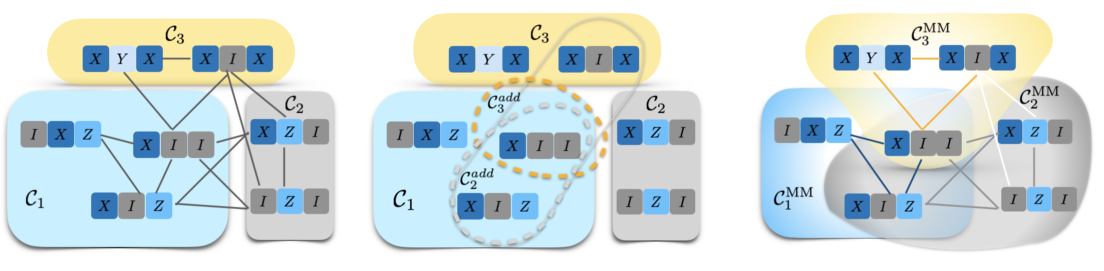
Figure 1: A graphical illustration of our Max-Min grouping protocol. Each vertex represents a Pauli observable, with individual Pauli operators denoted by squares of varying colors. Left [Equation 3: Minimize]: solid lines connect vertices that commute with each other. One of the minimum clique covers is depicted, with operators within the same shadows belonging to the same group $(\mathcal{C}_{\alpha})_{\alpha=1,2,3}$. Middle [Equation 4: Maximize]: the process of maximizing overlaps between groups to obtain $\mathcal{C}^{\mathrm{MM}}_{\alpha}$ is shown. In this example, operators inside the solid gray line are all operators that commute with $\mathcal{C}_{2}$, and the maximum clique of those operators that commute with each other (inside the gray dashed line) is the $\mathcal{C}_{2}^{\mathrm{add}}$ we are looking for to include into $\mathcal{C}_{2}$, and so it is with $\mathcal{C}_{3}^{\mathrm{add}}$ (circled by the yellow dashed line). Right [Equation 5]: the overlapped shaded region $\mathcal{C}_{2}^{\mathrm{add}}$ includes operators in $\mathcal{C}_{1}$ that also commute with all operators in $\mathcal{C}_{1}^{\mathrm{MM}}=\mathcal{C}_{1}$ and $\mathcal{C}_{2,3}^{\mathrm{MM}}=\mathcal{C}_{2,3}\cup\mathcal{C}_{2,3}^{\mathrm{add}}$. The Pauli gates associated with group $\mathcal{C}_{1,2,3}$ are $\mathcal{P}_{1}=X_{1}\otimes X_{2}\otimes Z_{3}$, $\mathcal{P}_{2}=X_{1}\otimes Z_{2}\otimes I_{3}$ and $\mathcal{P}_{3}=X_{1}\otimes Y_{2}\otimes X_{3}$; however, with the maximization procedure considered, measurement gates for $\mathcal{C}^{\mathrm{MM}}_{2}$ will have a fixed measurement gate for the third qubit and changes to $\mathcal{P}_{2}=X_{1}\otimes Z_{2}\otimes Z_{3}$.

[t!] (MaxMin Grouping)

1Qubit Hamiltonian ${\mathcal{H}}=\sum_{\ell}a_{\ell}O_{\ell}$ with all terms $O_{\ell}$ Pauli operator.

2MaxMin groups $\{\mathcal{C}^{\mathrm{MM}}_{\alpha}\}$ of all terms $\{O_{\ell}\}$ in ${\mathcal{H}}$.

3QWC Graph: Construct the QWC graph $G=(\{O_{l}\},\mathcal{Q}_{c})$

4Minimize: Apply a minimum clique cover solver [9] to $G$ output $\{\mathcal{C}_{\alpha}\}_{1\leq\alpha\leq A}$

5for $\alpha=1$ to $A$ do $\triangleright$ loop of over groups $\mathcal{C}_{\alpha}$

6    initialize $\mathcal{C}_{\alpha}^{\mathrm{QWC}}=[\leavevmode\nobreak\ ]$,

7    while $O_{\ell}\notin\mathcal{C}_{\alpha}$ do $\triangleright$ loop over $O_{\ell}\notin\mathcal{C}_{\alpha}$

8         if $O_{\ell}$ qubit-wise commutes with $\mathcal{P}_{\alpha}$  then

9             append $O_{\ell}$ to $\mathcal{C}_{\alpha}^{\mathrm{QWC}}$

10         end if

11    end while

12    Apply a maximum clique solver [25] to $\mathcal{C}_{\alpha}^{\mathrm{QWC}}$, output $\mathcal{C}_{\alpha}^{\mathrm{add}}$.

13    Maximize: $\mathcal{C}_{\alpha}^{\mathrm{MM}}=\mathcal{C}_{\alpha}.\mathrm{Append}[\mathcal{C}_{\alpha}^{\mathrm{add}}]$

14end for

The maximize process mainly helps us decide the measurement gates of qubits that have not been assigned by the minimize procedure. For example, in Fig. 1, the Pauli gates associated with $\mathcal{C}_{2}$ is changed from $X_{1}\otimes Z_{2}\otimes I_{3}$ to $X_{1}\otimes Z_{2}\otimes Z_{3}$ upon including $\mathcal{C}_{2}^{\mathrm{add}}$. This max-min grouping procedure ensures full utilization of each measurement. This maximization step is realized in Section 3.1 through steps $3$ to $12$. When we perform measurement for the group $\alpha$, using the measurement gates $\mathcal{P}_{\alpha}$, an operator will be measured if it belongs to the group $\alpha$. The overlap maximization step in our approach can increase the hit rates of observables that belong to the overlaps between operator groups. By maximizing the overlap, we ensure that the observables are measured more frequently within a fixed measurement budget, thereby improving the overall estimation accuracy. In general, this procedure guarantees high hit rates on observables, which is crucial for achieving precise estimates of the target quantities. The next task is to allocate measurement resources to each group to minimize the error.

3.2 Confidence Bound

Upon identifying the optimal operator grouping, our objective shifts toward determining the optimal allocation of measurement shots per group. Heuristically, assigning measurement budgets evenly across all the groups may seem reasonable, however, because a quantum Hamiltonian is a weighted average of Pauli observables, different operators would have varying importance to the accuracy of the energy estimation. Hence, allocating varying numbers of shots for different operator groups could potentially lead to more accurate estimation. Consequently, a cost function is imperative for guiding the allocation of shots to each group of observables.

Given the number of measurement shots $M$, we aim to achieve the most efficient group-wise measurement allocation, $\{M_{\alpha}\}$ with $\sum_{\alpha}M_{\alpha}=M$, minimizing the overall estimation error of the target Hamiltonian.

Consider the mean estimator for a Hamiltonian $\hat{{\mathcal{H}}}:=\sum_{\ell}a_{\ell}\hat{O}_{\ell}$, where $\hat{O}_{\ell}$ is the expectation value estimator for $\langle O_{\ell}\rangle_{\rho}=\mathrm{Tr}(\rho O_{\ell})$. We group the operators into QWC max-min groups $\{\mathcal{C}^{\mathrm{MM}}_{\alpha}\}_{1\leq\alpha\leq A}$. Our goal is to find the optimal allocation of measurement shots per group, denoted by $w_{\alpha}$. The expectation value of the Hamiltonian is then estimated by averaging the corresponding measurement outcomes. In practice, we use the median-of-means estimator (see Eq. 28) as the mean estimator for $\langle{\mathcal{H}}\rangle_{\rho}$, with details provided in Appendix B. The following theorem introduces a confidence bound that limits the error in the Hamiltonian expectation value for shots allocated to the max-min groups.

Theorem 1.

(Confidence bound) Suppose that a set of group $\{\mathcal{C}^{\mathrm{MM}}_{\alpha}\}_{1\leq\alpha\leq A}$ given as a set of max-min groups $\{C_{\alpha}^{\mathrm{MM}}\}$ of a set of Pauli observables $\{O_{\ell}\}_{\ell\leq L}$ of Hamiltonian ${\mathcal{H}}=\sum_{\ell}a_{\ell}O_{\ell}$, and a list assigns measurements to each group $\{w_{\alpha}\}$, and accuracy parameters $\epsilon,\delta$, s.t.

$$\mathrm{Conf}\left[\epsilon,\{w_{\alpha}\};M,\{C_{\alpha}^{\mathrm{MM}}\}\right]:=$$

$$2\sum_{\ell=1}^{L}\exp\left(-\frac{\epsilon^{2}M}{2(\sum_{\ell}|a_{\ell}|)^{2}}\sum_{\alpha=1}^{A}\mathrm{idx}_{\ell,\alpha}\;w_{\alpha}\right)=\delta$$ (6)

which subjected to $\sum_{\alpha}w_{\alpha}=1$.

The indicator $\mathrm{idx}_{\ell,\alpha}$ is define as

$$\mathrm{idx}_{\ell,\alpha}=\left\{\begin{array}[]{ll}1\nobreak\leavevmode\nobreak\leavevmode\nobreak\leavevmode\nobreak\leavevmode\nobreak\leavevmode&\text{if }O_{\ell}\in\mathcal{C}^{\mathrm{MM}}_{\alpha}\\ 0&\text{otherwise}\end{array}\right.$$ (9)

Then, a collection of $M$ independent classical shadows allows for accurately predicting the expectation Hamiltonian for the given quantum state $\rho$:

$$\left|\hat{{\mathcal{H}}}-\langle{\mathcal{H}}\rangle_{\rho}\right|\leq\epsilon$$ (10)

with probability $1-\delta$.

The detailed proof is provided in Appendix A. It should be highlighted that our proof adopts a similar process to the original classical shadow protocol in measuring a set of operators. We establish error bounds for each operator, and the bound on the Hamiltonian, which is the weighted sum of all observables, is derived using the union bound over all operators. This approach is analogous to the classical shadow protocol, where the error bounds are derived for each individual observable, and the overall error bound is obtained by applying the union bound.

This confidence bound serves as an overall cost function for our measurement resource allocation, where $\epsilon$ represents the error bound of the Hamiltonian. When quantum resources are limited, minimizing the cost function leads to a concentration of measurements on a few groups, i.e., groups containing a large number of observables. In such cases, it is possible for the cost function to exceed one, causing the confidence bound to break down. However, this is acceptable since the confidence bound acts as a cost function for shot allocation under limited quantum resources, and it is crucial to recognize that in these situations, accuracy is not guaranteed. The confidence bound is used as a guide for optimizing the measurement allocation, rather than as a strict guarantee on the estimation error.

In most scenarios, the confidence bound provided in Theorem 1 offers an effective guide for optimizing the allocation of measurement resources across groups, prioritizing the overall accuracy of the Hamiltonian estimation. However, in certain extreme cases, such as when a Hamiltonian contains groups with significantly imbalanced sizes and coefficient magnitudes (see Section A.2.1). the confidence bound in Theorem 1 may not provide the optimal allocation. In such cases, the supplementary confidence bound introduced in Section A.2 can be more useful. This alternative bound takes into account the coefficients of the observables within each group, allowing for a more nuanced allocation of measurement resources. By considering each group’s relative importance based on its size and the magnitudes of its observable coefficients, the supplementary confidence bound can help mitigate the potential breakdown of the primary bound in these extreme scenarios. Nonetheless, for most practical applications, the confidence bound in Theorem 1 remains a robust and reliable tool for guiding the measurement optimization process.

3.3 Measurement Resource Allocation

Given the confidence bound proposed in  Theorem 1, which is used as a cost function, the next step involves solving the measurement resource allocation problem by minimizing the confidence bound, which is presented in Algorithm 3.3. By optimizing the allocation of measurement resources based on the confidence bound, we aim to achieve the best possible estimation accuracy given the available quantum resources, even if the confidence bound itself may not always provide a tight error guarantee.

[t!]

(ROGS)

1Measurement budget $M$, accuracy parameter $\epsilon$, and Hamiltonian ${\mathcal{H}}=\sum_{\ell}a_{\ell}O_{\ell}$.

2A fixed Pauli basis measurement recipe $\{\mathcal{P}_{\alpha}^{\otimes M_{\alpha}}\}_{1\leq\alpha\leq A}\in\{X,Y,Z\}^{n\times M}$ for the classical shadow quantum measurement stage.

3Identify the max-min groups $\{C_{\alpha}^{\mathrm{MM}}\}$ of operators $\{O_{\ell}\}$ in ${\mathcal{H}}$ using Algorithm 3.1.

4Apply a convex optimization solver to find the optimal distribution $\{w_{\alpha}\}$ of measurements among groups to minimize the confidence bound,

$$\{w_{\alpha}^{*}\}=\arg\min_{\{w_{\alpha}\}}\mathrm{Conf}\left[\epsilon,\{w_{\alpha}\};M,\{C_{\alpha}^{\mathrm{MM}}\}\right].$$ (11)

5Obtain measurement recipes $\{\mathcal{P}_{\alpha}^{\otimes M_{\alpha}}\}_{1\leq\alpha\leq A}$ which include $\{X,Y,Z\}^{n\times M}$ based on $\{M_{\alpha}\}:=\{[w_{\alpha}^{*}M]\}$ and one to one correspondence between groups $\{\mathcal{C}_{\alpha}^{\mathrm{MM}}\}$ and Pauli measurement gates $\mathcal{P}_{\alpha}$.

Measurement Resource Allocation via Convex Optimization. Now, we can determine the allocation of the measurement budget among groups based on the confidence bound (1) derived in Theorem 1. Note that the confidence bound can be transformed into a log-sum-exp function, which is smooth and convex. Minimization of this function can be efficiently performed by a convex optimization solver (e.g., CVXPY [26]), which outputs a set of optimal weights $\{w_{\alpha}\}$ for shot allocation to each group. We demonstrate the whole process in Section 3.3, which takes a measurement budget $M$ and outputs measurement recipes, $\{\{\mathcal{P}^{(m)}_{\alpha}\}_{1\leq m\leq M_{\alpha}}\}$.

4 Results

In this section, we focus on estimating the ground state energy of small molecules with various encoding schemes: Jordan-Wigner (JW) [27], Bravyi-Kitaev (BK) [6], and Parity (P) [6, 7]. These schemes transform the fermionic Hamiltonian of a specified molecule into qubit Hamiltonians, represented as weighted sums of Pauli operators. We benchmark against the exact calculation of their ground state energy by diagonalization of the Hamiltonians.

4.1 Implementation

We obtain the qubit Hamiltonians of benchmark molecules with various encodings via Qiskit [28] and diagonalize these Hamiltonians numerically to obtain the corresponding ground states using SciPy [29]. For the Max-Min grouping stage, the minimum clique cover is obtained via Qiskit as well, and the maximum cliques are found by solvers from NetworkX [30]. In the measurement resource allocation stage, we adopt the convex optimization solver from CVXPY [26]. Finally, we perform circuit simulations with the PennyLane lightning simulator [31].

4.2 Results

In Table 1, we benchmark ROGS against other measurement techniques for various small molecules ($\mathrm{H_{2}}$, $\mathrm{LiH}$, $\mathrm{BeH_{2}}$, $\mathrm{H_{2}O}$, $\mathrm{NH_{3}}$) using the three encoding schemes. Each algorithm was allocated an equal number of measurement shots to compute the average error $|\hat{{\mathcal{H}}}-\langle{\mathcal{H}}\rangle_{\rho}|$. Through ten simulations and the subsequent calculation of their root mean square deviation, it is evident that the ROGS technique results in a lower estimation error compared to other methods. Notably, the ROGS approach often exceeds the performance of alternative strategies while requiring significantly fewer measurement circuits (see Table 1), demonstrating its efficient allocation of selective measurement resources. A key observation is that, with limited measurement shots, molecules with a larger number of operators and a greater number of mutually non-commuting groups tend to require measuring the same or even fewer groups. This occurs because, under a limited budget, accuracy is higher when focusing on the estimation of groups with more operators rather than measuring all groups with very few shots. This phenomenon illustrates the bias-variance tradeoff [32], which can be interpreted using the concept of mean-field theory as we consider the high-weighted groups as the mean-field subspace that captures the dominant interactions within the system, which is detailed in Section 5. ROGS performance is similar to the recently proposed method, adaptive estimation of quantum observables (AEQuO) [20]. This method also seeks to optimally allocate measurements to overlapping groups. However, AEQuO allocates shots to minimize the variance of the target observable, as opposed to ROGS which minimizes the confidence bound in Theorem 1.

Molecule ($L$)	Enc.	$n_{\mathrm{groups}}$	ROGS	Derand.	APS	OGM	AEQuO
$\mathrm{H_{2}}$ (185)	JW	46	6	159	217	37	40
	P	34	5	77	116	39	30
	BK	34	8	66	114	33	26
$\mathrm{LiH}$ (631)	JW	136	11	643	259	63	126
	P	165	41	534	177	78	126
	BK	211	2	661	237	57	136
$\mathrm{BeH_{2}}$ (666)	JW	140	24	624	462	56	126
	P	177	10	630	310	76	115
	BK	193	10	671	300	80	110
$\mathrm{H_{2}O}$ (1086)	JW	224	41	781	560	32	171
	P	260	3	774	415	57	174
	BK	303	5	786	319	48	172
$\mathrm{NH_{3}}$ (3057)	JW	618	5	962	776	39	287
	P	720	3	956	568	79	298
	BK	729	7	987	623	60	280

Table 1: Empirical circuit cost benchmark: This table shows the comparison of the number of circuits $n_{\mathrm{circuit}}$ required for estimating the ground states using a measurement budget of 1,000 shots of benchmark molecules (each with $L$ Pauli operators) across different encoding schemes: JW, P, and BK. The column labeled $n_{\mathrm{groups}}$ indicates the total number of overlapping groups, while the $n_{\mathrm{circuit}}$ column shows the significantly reduced number of circuits achieved with the grouping shadow technique. The abbreviations used are as follows: ROGS, derandomized classical shadow (Derand.) [15], Adaptive Pauli Shadow (APS) [17], overlapped grouping measurement (OGM) [19], and adaptive estimation of quantum observables (AEQuO) [20].

Molecule ($E_{\mathrm{GS}}$)	Enc.	ROGS	Derand.	APS	OGM	AEQuO
$\mathrm{H_{2}}$ $(-1.86)$	JW	0.03	0.06	0.07	0.05	0.03
	P	0.01	0.03	0.05	0.06	0.02
	BK	0.02	0.06	0.08	0.05	0.02
$\mathrm{LiH}$ $(-8.91)$	JW	0.02	0.03	0.04	0.04	0.02
	P	0.02	0.03	0.05	0.04	0.02
	BK	0.01	0.04	0.07	0.04	0.02
$\mathrm{BeH_{2}}$ $(-19.04)$	JW	0.02	0.06	0.06	0.07	0.04
	P	0.03	0.09	0.06	0.08	0.04
	BK	0.04	0.06	0.06	0.06	0.04
$\mathrm{H_{2}O}$ $(-83.60)$	JW	0.09	0.12	0.11	0.13	0.09
	P	0.08	0.22	0.11	0.20	0.07
	BK	0.07	0.20	0.10	0.15	0.10
$\mathrm{NH_{3}}$ $(-66.88)$	JW	0.09	0.18	0.13	0.15	0.10
	P	0.09	0.21	0.14	0.12	0.12
	BK	0.08	0.12	0.11	0.14	0.11

Table 2: Empirical benchmark: This table shows the average estimation error (RMSE) across various molecules, encodings, and measurement strategies. The RMSE is calculated by simulating the process 10 times, each with 1,000 measurements. The first column details the molecule, along with its ground state electronic energy expressed in Hartree units.

In Figure 2, we show the energy estimation with error bars for the molecule $\mathrm{LiH}$ using the BK encoding scheme. While all techniques have reasonable accuracy, ROGS in particular has a much smaller variance due to the deterministic allocation of measurements with convex optimization. This is an example of the bias-variance tradeoff. In Figure 3, we show the quantum resource efficiency of ROGS for ground state energy estimation of small molecules ($\mathrm{H_{2}}$, $\mathrm{LiH}$, $\mathrm{BeH_{2}}$) using the BK encoding. ROGS consistently achieves target accuracies with the fewest shots and unique circuits compared to the derandomized classical shadow and AEQuO methods. The efficiency advantage of ROGS becomes more pronounced as the number of qubits increases. Interestingly, ROGS requires fewer shots for $\mathrm{LiH}$ than $\mathrm{H_{2}}$, despite the latter having a smaller Hilbert space. This is due to the highly localized mean-field subspace (detailed in Section 5) and low one-shot variance of operator expectation estimation in $\mathrm{LiH}$. By minimizing both the number of measurements and distinct circuits, ROGS addresses the significant overhead in compiling and loading circuits on quantum hardware, enabling more efficient characterization of molecular systems.

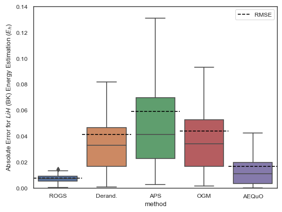
Figure 2: Estimation Accuracy of Ground State Energy for $\mathrm{LiH}$ with Bravyi-Kitaev Encoding [6] using various measurement strategies. This figure shows box plot of the absolute error of ground state energy estimations across 50 independent runs, each with 1,000 measurements. We compare ROGS with several methods: Derandomized Classical Shadow (Derand.) [15], Adaptive Pauli Shadow (APS) [17], Overlapped Grouping Measurement (OGM) [19], and adaptive estimation of quantum observables (AEQuO) [20]. The solid line in the bar plot represents the mean, while the dashed line represents the root mean square error.

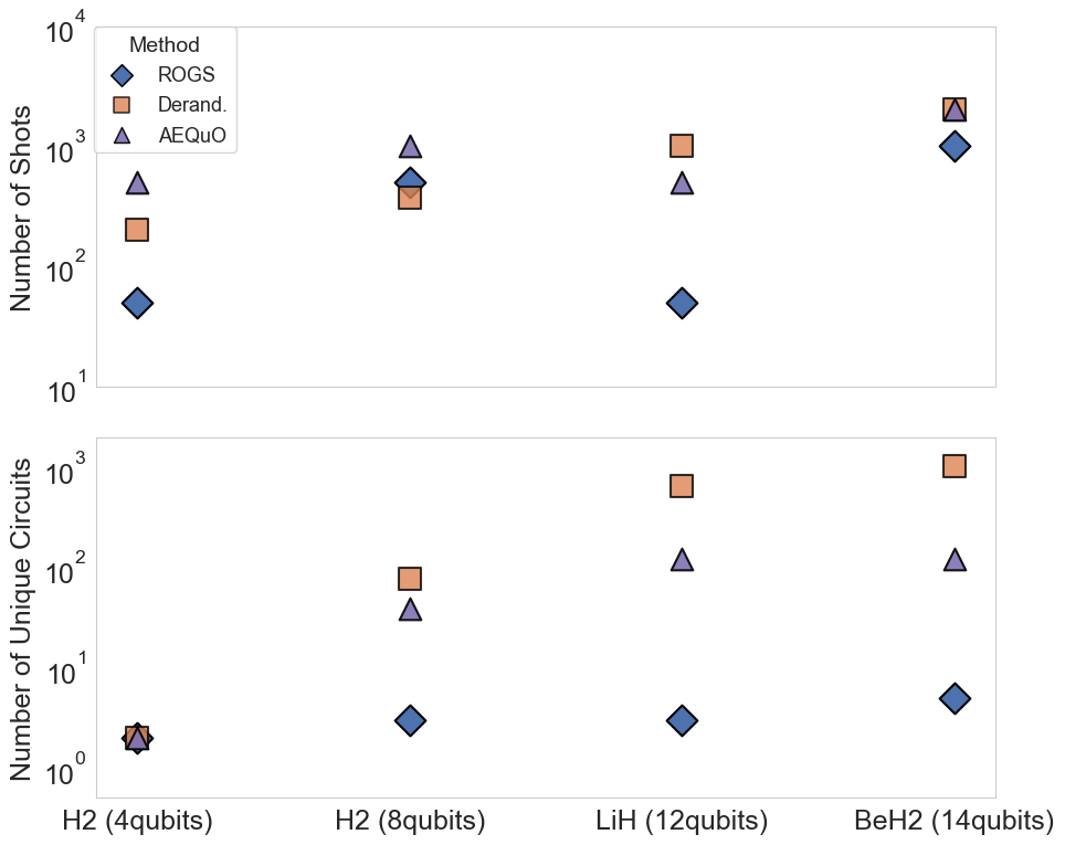
Figure 3: Quantum Resource Efficiency of Ground State Energy Estimation for various molecules using the Bravyi-Kitaev encoding [6]. The upper plot shows the number of shots (quantum circuit executions), while the lower plot displays the number of unique quantum circuits required to reach a target accuracy of 0.03 Hartree ($E_{h}$) for different molecules and measurement strategies: ROGS (blue $\Diamond$), Derandomized Classical Shadow (Derand., orange $\square$), and adaptive estimation of quantum observables (AEQuO, purple $\triangle$).

As the provision of quantum resources increases, these resources tend to be distributed more evenly across all groups, as illustrated in Fig. 4 using $\mathrm{H_{2}}$ (encoding: BK, basis: 6-31g) as an example. It is observed that the number of groups measured increases from six high-weighted groups to encompassing all groups. When the measurement resource is limited, the global optimum of the confidence bound concentrates resources on a subset of groups, which is beneficial due to the bias-variance tradeoff. This concentration of shots in high-importance groups diminishes as the available quantum resources increase. In the limit of infinite measurement shots, all observables must be estimated accurately to minimize the total estimation error. This is due to each group containing at least one unique Pauli observable that cannot be covered by the group maximization procedure. Consequently, as the number of shots approaches infinity, the allocation of shots across groups becomes more uniform to ensure that all observables are measured with enough resources. This behavior ensures that the estimation error of the Hamiltonian is minimized by accurately estimating all of its constituent observables, regardless of their distribution among the groups.

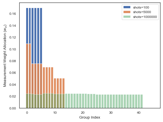
Figure 4: Shot Allocation for $\mathrm{H_{2}}$ Using Jordan-Wigner [27] (JW) Encoding Across Varying Total Number of Experiments. This plot illustrates the allocation of shots as determined by convex optimization of the confidence bound (Theorem 1) for a specified $\epsilon$ over different total numbers of measurements $M$. It can be observed that with the total measurement shots $M$ increasing, the allocation of measurement weights across groups becomes more uniform.

It is worth noting that the MCC problem is an NP-hard problem and is typically solved by applying heuristic algorithms [9], which do not guarantee to find the true minimum clique cover. The minimum clique cover found by [9] for $\mathrm{H_{2}}$ (encoding: BK, basis: 6-31g) results in $n_{\mathrm{groups}}=46$ qubit-wise commuting groups (see Table 1). However, this number is over-counted, and in this example, four of the groups do not contain any unique Pauli operators, i.e., operators that belong only to a single group. In our shot allocation determined by Theorem 1, one can observe that no shots are allocated to these groups, even when more than enough quantum resources are provided (see Figure 4). This suggests that our approach based on Theorem 1 could potentially provide a closer approximation to the optimal MCC solution by effectively identifying and excluding redundant groups that do not contribute much to the overall energy estimation.

5 Discussion

For the numerical experiments presented in Section 4, it is found that excellent results can be achieved by measuring very few groups (fewer than the total number of groups, see Table 1). This is attributed to the fact that with a fixed measurement budget, omitting certain groups with insufficient measurements can significantly reduce the estimation variance at the cost of an increased bias in estimation. This tradeoff, widely recognized as the bias-variance tradeoff in the statistics community (see, for instance, Sec. 2.2.2 of Ref. [32]), has been shown to be beneficial for mean estimation with finite samples.

Physical Interpretation. from a physical standpoint: each group $\mathcal{C}_{\alpha}^{\mathrm{MM}}$ can be viewed as a mean-field subspace of the Hamiltonian [33]. These subspaces are constructed by maximizing the number of mutually commuting operators within each group, essentially capturing the local mean-field interactions among the qubits. The mean-field approximation is often used to describe systems where the interactions between particles can be effectively averaged out, leading to a simplified description of the system. In the context of the overlapped grouping protocol (Sec. 3.1), the larger groups with more mutually commuting operators can be seen as capturing these averaged interactions, providing a good approximation of the overall system behavior.

It is worth pointing out that the mean-field subspaces identified by ROGS not only correspond to groups with a large number of operators but also account for the magnitude of the coefficients associated with these operators. In the context of electronic structure Hamiltonians, the coefficients of Pauli operators can vary significantly, with some terms having much larger coefficients than others. As demonstrated in [33], these large coefficient terms often capture the dominant mean-field interactions within the system. Therefore, the high-weight groups in ROGS are those that contain either a large number of operators or operators with very large coefficients, or both.

When we have a limited number of measurements, allocating more resources to these mean-field subspaces allows us to better capture the dominant interactions within the system. By focusing on these larger groups, we are effectively prioritizing the measurement of the most significant contributions to the overall Hamiltonian. On the other hand, distributing the measurements evenly across all groups, including those with fewer operators, will lead to a less accurate representation of the system (see results in Table 3 Even distribution). This is because the smaller groups may contain less significant interactions or may represent more local, "fluctuation" terms that deviate from the mean-field approximation.

By allocating more measurement resources to these mean-field subspaces, we are essentially focusing on the most relevant parts of the Hamiltonian that contribute to the overall system properties. This approach allows us to obtain excellent results with fewer measured groups, as the dominant interactions are well-captured within these larger mean-field subspaces. Hence the mean-field interpretation suggests that concentrating measurements on groups with more operators (i.e., larger mean-field subspaces) is an effective strategy when dealing with limited resources. In this approach, with limited measurement resource, we mainly the capture of the most significant interactions within the system, leading to accurate results while measuring fewer groups overall. The bias-variance tradeoff can be seen as a manifestation of this mean-field approximation, where focusing on the dominant mean-field subspaces reduces the variance in the measurement results at the cost of potentially introducing some bias by neglecting the smaller fluctuation terms.

6 Conclusion and Outlook

In this work, we introduce a novel method, Resource-Optimized Grouping Shadow (ROGS), for efficiently estimating the expectation values of a set of Pauli observables on a quantum state. The key idea is to allocate the limited measurement budget to fewer unique circuits, each corresponding to a group of commuting Pauli observables. Specifically, when the total number of measurements is limited, minimizing the confidence bound tends to allocate more resources to the high-weight groups, i.e., groups containing a larger number of commuting Pauli observables or with large coefficients, while potentially omitting measurements on some low-weight groups. This selective measurement strategy effectively minimizes the variance in the energy estimation. Notably, ROGS can significantly reduce the number of circuits prepared for measurements, which is a critical cost factor for tasks running on modern quantum computers.

The resource allocation strategy in ROGS can be interpreted using the concept of mean-field theory. In this context, the high-weight groups can be viewed as capturing the dominant mean-field interactions within the quantum system, while the low-weight groups represent local fluctuations that deviate from the mean-field approximation. By allocating more measurement resources to the larger mean-field subspaces (high-weight groups), ROGS prioritizes the measurement of the most significant contributions to the overall Hamiltonian. In contrast, distributing the measurements evenly across all groups, including those with fewer observables (low-weight groups), may lead to a less accurate representation of the system, as these groups may contain less significant interactions or local fluctuations. ROGS could have significant implications for VQE. In VQE, the objective function is the energy of a target system, which is the expectation value of the system’s Hamiltonian expressed as a weighted sum of Pauli operators. The gradient calculation for the variational quantum circuit in VQE can be completed using the parameter-shift approach [34], which involves estimating the energy for the circuit under different parameter perturbations. Evidently, ROGS can be applied to each energy estimation procedure, thereby benefiting the gradient estimation task in VQE.

Incorporating non-QWC commuting terms [35] will push the boundaries of measurement reduction even further. This research direction has the potential to significantly decrease the required number of quantum measurements, making the characterization of larger-scale quantum systems more feasible. Furthermore, this approach aligns well with the mean-field [33] interpretation discussed earlier. By grouping commuting terms that span across different qubits, we can capture longer-range correlations and interactions within the system. This may lead to a more accurate representation of the system’s properties while still benefiting from the measurement efficiency gains provided by the overlapped grouping protocol.

Although we refer to our method as a shadow method, which acts as a pre-processing stage of classical shadow protocol to produce deterministic measurement bases before the quantum measurements, the techniques introduced here have potential applications beyond classical shadows. The optimal allocation of measurement resources and the Max-Min grouping strategy could be beneficial in other areas of quantum computing, such as VQE and gradient estimation, especially considering that ROGS could be used in energy estimation for any state including the ground state. These techniques may help enhance the efficiency of algorithms involving weighted sums of Pauli observables, similar to the Hamiltonian in the shadow method. Therefore, the insights gained from this work may have broader implications for various quantum computing applications.

Appendix A Confidence bound

A.1 Proof of Theorem 1

In this section, we will provide a comprehensive proof of Theorem 1, which establishes the confidence bound for accurately predicting the expectation value of the Hamiltonian.

Proof.

Based on triangle inequality, one has the Hamiltonian upper bounded by

$$\left|\hat{{\mathcal{H}}}-\langle{\mathcal{H}}\rangle_{\rho}\right|=\left|\sum_{\ell}a_{\ell}(\hat{O}_{\ell}-\langle O_{\ell}\rangle_{\rho})\right|\leq\sum_{\ell}|a_{\ell}|\left|\hat{O}_{\ell}-\langle O_{\ell}\rangle_{\rho}\right|\leq(\sum_{\ell}|a_{\ell}|)\max_{\ell}\left|\hat{O}_{\ell}-\langle O_{\ell}\rangle_{\rho}\right|$$ (12)

It is equal to prove that the maximum group’s expectation value is upper bounded, i.e.

$$\mathrm{Pr}\left[\max_{\ell}\left|\hat{O}_{\ell}-\langle O_{\ell}\rangle_{\rho}\right|\geq\epsilon/\sum_{\ell}|a_{\ell}|\right]=\mathrm{Pr}\left[\bigcup_{\ell}\left|\hat{O}_{\ell}-\langle O_{\ell}\rangle_{\rho}\right|\geq\epsilon/\sum_{\ell}|a_{\ell}|\right]$$

$$\leavevmode\nobreak\ \leavevmode\nobreak\ \leavevmode\nobreak\ \leavevmode\nobreak\ \leavevmode\nobreak\ \leavevmode\nobreak\ \leavevmode\nobreak\ \leavevmode\nobreak\ \leavevmode\nobreak\ \leavevmode\nobreak\ \leavevmode\nobreak\ \leavevmode\nobreak\ \leavevmode\nobreak\ \leavevmode\nobreak\ \leavevmode\nobreak\ \leavevmode\nobreak\ \leavevmode\nobreak\ \leavevmode\nobreak\ \leavevmode\nobreak\ \leavevmode\nobreak\ \leavevmode\nobreak\ \leavevmode\nobreak\ \leavevmode\nobreak\ \leavevmode\nobreak\ \leavevmode\nobreak\ \leavevmode\nobreak\ \leavevmode\nobreak\ \leavevmode\nobreak\ \leavevmode\nobreak\ \leavevmode\nobreak\ \leavevmode\nobreak\ \leavevmode\nobreak\ \leavevmode\nobreak\ \leavevmode\nobreak\ \leavevmode\nobreak\ \leavevmode\nobreak\ \leavevmode\nobreak\ \leavevmode\nobreak\ \leavevmode\nobreak\ \leavevmode\nobreak\ \leavevmode\nobreak\ \leavevmode\nobreak\ \leavevmode\nobreak\ \leavevmode\nobreak\ \leavevmode\nobreak\ \leavevmode\nobreak\ \leavevmode\nobreak\ \leavevmode\nobreak\ \leavevmode\nobreak\ \leavevmode\nobreak\ \leavevmode\nobreak\ \leavevmode\nobreak\ \leavevmode\nobreak\ \leavevmode\nobreak\ \leavevmode\nobreak\ \leavevmode\nobreak\ \leavevmode\nobreak\ \leavevmode\nobreak\ \leavevmode\nobreak\ \leq\sum^{L}_{\ell=1}\mathrm{Pr}\left[\left|\hat{O}_{\ell}-\langle O_{\ell}\rangle_{\rho}\right|\geq\epsilon/\sum_{\ell}|a_{\ell}|\right]$$ (13)

The inequality arises from the union bound – also known as Boole’s inequality – which states that the probability associated with a union of events is upper bounded by the sum of individual event probabilities. We can evaluate the individual group error rate probability separately. We evaluate the expectation of operators $\{O_{\ell}\}$ by averaging over the measurement results of the circuit. Let ${{q_{j}[m]}_{j\leq n}}_{m\leq M_{\alpha}}$ is a list of computational basis measurement results on each qubit, where $j$ is the qubit site and $m$ is the $m$th measurement, then the shadow estimation expectation value of operator $O_{\ell}$ is defined by average overall measurement results on this operator: $\hat{O}_{\ell}=M_{\alpha}^{-1}\sum_{m=1}^{M_{\alpha}}s_{m}^{(\ell)}$, where $s_{m}^{(\ell)}$ is a sign defined by the z-basis measurement result on each site within the support of that observable ${\pm 1}\ni s_{m}^{(\ell)}:=\prod_{j\in\mathrm{supp}\{O_{\ell}\}}q_{j}[m]$. One could expect that we can get the operator exact expectation value by taking infinite measurement: $\langle O_{\ell}\rangle_{\rho}=\lim_{M_{\alpha}\rightarrow\infty}\hat{O}_{\ell}\equiv\mathbb{E}(s_{m}^{(\ell)})$, then the individual term of the sum in (A.1) can be written as:

$$\mathrm{Pr}\left[\left|\frac{1}{M_{\alpha}}\sum_{m=1}^{M_{\alpha}}(s_{m}^{(\ell)}-\mathrm{E}[s_{m}^{(\ell)}])\right|\geq\frac{\epsilon}{\sum_{\ell}|a_{\ell}|}\right]\leq 2\sum_{\ell}\exp\left(-\frac{\epsilon^{\prime 2}M_{\ell}}{2}\right)$$ (14)

The last inequality follows from Hoeffding’s inequality since each measurement result can be taken as an independent event and independent random variables, $s_{m}^{(\ell)}\in\{-1,1\}$. The number of measurements performed on each operator is the sum of the shots allocated to groups to which the operator belongs, i.e., $M_{\ell}=\sum_{\alpha,O_{\ell}\in\mathcal{C}^{\mathrm{MM}}_{\alpha}}M_{\alpha}$; adopting the indicator $\mathrm{idx}_{\ell,\alpha}$ as defined in Theorem 1, we have $M_{\ell}=\sum_{\alpha=1}^{A}\mathrm{idx}_{\ell,\alpha}M_{\alpha}=M\sum_{\alpha=1}^{A}\mathrm{idx}_{\ell,\alpha}w_{\alpha}$, where $w_{\alpha}=M_{\alpha}/M$ is the shots weight of group $\mathcal{C}_{\alpha}^{\mathrm{MM}}$.

Therefore, one can accurately predict Hamiltonian:

$$\left|\hat{{\mathcal{H}}}-\langle{\mathcal{H}}\rangle_{\rho}\right|\leq\epsilon$$ (15)

with accuracy $1-\delta$, where

$$\delta=2\sum_{\ell=1}^{L}\exp\left(-\frac{\epsilon^{2}M\sum_{\alpha}\mathrm{idx}_{\ell,\alpha}w_{\alpha}}{2(\sum_{\ell}|a_{\ell}|)^{2}}\right)\geq\mathrm{Pr}\left[\max_{\ell}\left|\hat{O}_{\ell}-\langle O_{\ell}\rangle_{\rho}\right|\geq\epsilon/(\sum_{\ell}|a_{\ell}|)\right],\leavevmode\nobreak\ \leavevmode\nobreak\ \sum_{\alpha}w_{\alpha}=1.$$ (16)

∎

Remarks. We can find a shot allocation $\{M_{\alpha}\}$ is allocated among the overlapped groups $\{\mathcal{C}_{\alpha}^{\mathrm{MM}}\}$ given the total number of measurement budgets $M$, where $M=\sum_{\alpha}M_{\alpha}$, to minimize the confidence bound 1 through convex optimization of a Log-Sum-Exp type function. However, note that although $\epsilon$ is the error bound in the tail bounds, it functions as a hyperparameter in the convex optimization problem, meaning that for each $\epsilon$, there is corresponding minimum confidence bound $\delta$ as indicated in (16), while the optimized result, or shots allocation $\{w_{\alpha}\}$, remains unchanged provided that $\epsilon^{2}M$ is constant. Therefore, one should aim to find the optimal $\epsilon_{0}$ for a small budget $M_{0}$, keeping the hyperparameter $\epsilon_{0}^{2}M_{0}$ fixed, i.e., for any total budget $M$, one would choose $\epsilon=\epsilon_{0}\sqrt{M_{0}/M}$ to achieve the optimal measurement result, which is the core concept of algorithm 3.3.

Eq. (16) gives confidence bound for the estimation of the Hamiltonian’s expectation value when each observable $O_{l}$ is estimated with $M_{\ell}=M\sum_{\alpha=1}^{A}\mathrm{idx}_{\ell,\alpha}w_{\alpha}$ measurement shots. On the other hand, as the total number of shots $M$ is fixed, the various choices of the weights $\{w_{\alpha}\}$ lead to different $\delta$. As the lower $\delta$ leads to higher confidence, we want to find the optimal choice of $\{w_{\alpha}\}$ under constraint $\sum w_{\alpha}=1$ to minimize the hyperparameter $\delta$.

A.2 Comparison between confidence bound

This subsection introduces a supplementary confidence bound. This modification from the previously discussed confidence bound aims to address scenarios where groups with larger numbers of terms but smaller average coefficients are compared against groups with fewer terms but larger coefficients.

Apparently, the Hamiltonian can be grouped by $\mathcal{C}^{\mathrm{MM}}_{\alpha}$

$$\left|\hat{{\mathcal{H}}}-\langle{\mathcal{H}}\rangle_{\rho}\right|=\left|\sum_{\alpha=1}^{A}\sum_{O_{\ell}\in\mathcal{C}^{\mathrm{MM}}_{\alpha}}a_{\ell}(\hat{O}_{\ell}-\langle O_{\ell}\rangle_{\rho})\right|\leq\sum_{\alpha=1}^{A}\left|\sum_{O_{\ell}\in\mathcal{C}^{\mathrm{MM}}_{\alpha}}a_{\ell}w^{o}_{\ell,\alpha}(\hat{O}_{\ell}-\langle O_{\ell}\rangle_{\rho})\right|$$ (17)

where $w^{o}_{\ell,\alpha}$ is a weight distribution such that $w^{o}_{\ell,\alpha}\geq 0$, $\sum_{\alpha}w^{o}_{\ell,\alpha}=1$. One example is $w^{o}_{\ell,\alpha}=(\sum_{\alpha}\mathrm{idx}_{\ell,\alpha})^{-1}$. Therefore, one could apply a tail bound to the max-min group instead of the individual operators of the Hamiltonian. Similar to the previous section, one can upper-bound the error of the Hamiltonian by demonstrating that the maximum group’s expectation value has a high confidence level:

$$\mathrm{Pr}\left[\max_{\alpha}\left|\sum_{O_{\ell}\in\mathcal{C}^{\mathrm{MM}}_{\alpha}}\!\!{a_{\ell}}{w^{o}_{\ell,\alpha}}(\hat{O}_{\ell}-\langle O_{\ell}\rangle_{\rho})\right|\geq\epsilon/A\right]\leq\sum^{A}_{\alpha=1}\mathrm{Pr}\left[\left|\sum_{O_{\ell}\in\mathcal{C}^{\mathrm{MM}}_{\alpha}}\!\!a_{\ell}{w^{o}_{\ell,\alpha}}(\hat{O}_{\ell}-\langle O_{\ell}\rangle_{\rho})\right|\geq\epsilon/A\right]$$ (18)

based on the same argument as the previous section, one has

$$\mathrm{Pr}\left[\left|\sum_{O_{\ell}\in\mathcal{C}^{\mathrm{MM}}_{\alpha}}\frac{{a_{\ell}}{w^{o}_{\ell,\alpha}}}{M_{\alpha}}\sum_{m=1}^{M_{\alpha}}(s_{m}^{(\ell)}-\mathrm{E}[s_{m}^{(\ell)}])\right|\geq\frac{\epsilon}{A}\right]$$

$$=\mathrm{Pr}\left[\frac{1}{M_{\alpha}}\left|\sum_{m=1}^{M_{\alpha}}\left(\sum_{O_{\ell}\in\mathcal{C}^{\mathrm{MM}}_{\alpha}}{a_{\ell}}{w^{o}_{\ell,\alpha}}s_{m}^{(\ell)}-\mathbb{E}\left[\sum_{O_{\ell}\in\mathcal{C}^{\mathrm{MM}}_{\alpha}}{a_{\ell}}{w^{o}_{\ell,\alpha}}s_{m}^{(\ell)}\right]\right)\right|\geq\frac{\epsilon}{A}\right]$$ (19)

considered that each measurement result can be taken as an independent event and independent random variables $(X_{m})_{m\leq M_{\alpha}}$ are bounded s.t. $X_{m}:=\sum_{O_{\ell}\in\mathcal{C}^{\mathrm{MM}}_{\alpha}}{a_{\ell}}{w^{o}_{\ell,\alpha}}s_{m}^{(\ell)}\in[-\sum_{O_{\ell}\in\mathcal{C}^{\mathrm{MM}}_{\alpha}}{|a_{\ell}|}{w^{o}_{\ell,\alpha}},\sum_{O_{\ell}\in\mathcal{C}^{\mathrm{MM}}_{\alpha}}{|a_{\ell}|}{w^{o}_{\ell,\alpha}}$, therefore based on Hoeffding’s inequality, each group error probability is bounded by:

$$\mathrm{Pr}\left[\frac{1}{M_{\alpha}}\left|\sum_{m=1}^{M_{\alpha}}\left(X_{m}-\mathbb{E}\left[X_{m}\right]\right)\right|\geq\frac{\epsilon}{A}\right]\leq 2\exp\left(-\frac{\epsilon^{2}M_{\alpha}}{2(A\sum_{O_{\ell}\in\mathcal{C}^{\mathrm{MM}}_{\alpha}}{|a_{\ell}|}{w^{o}_{\ell,\alpha}})^{2}}\right)$$ (20)

by taking summation over all groups as in the previous section, one could obtain the confidence bound (16). This revised bound could provide a more equitable distribution among groups compared to the initial one, depending on the setting of weight parameter $w^{o}_{\ell,\alpha}$. If the measurement budget is not a constraint, this form of the confidence bound could be instrumental in deciding how shots are allocated among groups. For instance, by setting $w^{o}_{\ell,\alpha}$ as a constant concerning $\alpha$, i.e. $w^{o}_{\ell,\alpha}=1/\sum_{\alpha}\mathrm{idx}_{\ell,\alpha}$. In general, one might find beneficial results by setting it proportional to the number of operators within the respective group $w^{o}_{\ell,\alpha}\propto\sum_{\ell}\mathrm{idx}_{\ell,\alpha}$ or even setting $w^{o}_{\ell,\alpha}=0$ for all low-weighted groups (groups with a small number of operators or small absolute values of coefficients). This approach allows the operators to concentrate on high-weight groups, thereby expanding the main-field subspace. With finite quantum resources, this strategy helps focus resources on the most significant interactions within the system, thus dealing effectively with limited resources (see Section 3.3).

Remarks. Interestingly, the hyper-parameter $\epsilon^{2}M$ can be interpreted as an inverse temperature in a thermal state. At high temperatures, analogous to thermal agitation, the shots distribute more uniformly across the groups, resembling a system with a flattened Boltzmann distribution. Conversely, at low temperatures, the system approaches its thermal ground state, and the shots predominantly concentrate in high-weight groups, mimicking the population of low-energy states. This behavior is reminiscent of the Boltzmann distribution, where the probability of occupying a state decreases exponentially with its energy. By tuning the hyper-parameter $\epsilon^{2}M$, one can effectively control the "temperature" of the shot allocation, allowing for a balance between exploration and exploitation of the group weights.

Although this version of the confidence bound takes the effect of coefficients on operators into account, its overemphasis on coefficients can lead to less accurate estimations. This inaccuracy may arise from factors beyond just the coefficients; for example, the variance of the operators, which is state-dependent, also affects the estimation accuracy. An extreme example is the identity operator in a qubit Hamiltonian, which always has the largest coefficients among all operators but zero variance. Therefore, one can obtain the expectation value of the identity operator without any measurement, which is why we consider only the traceless Hamiltonian. The same argument applies to all operators: the variance does not depend on the coefficients but is instead state-dependent. Therefore, simply considering the coefficients as the measurement weight does not yield satisfactory results. It could be beneficial to take the variance of operators into account when we have some knowledge of the state after initial measurements (see Section A.3).

The supplementary confidence bound involves a more complex optimization process, where the weights $w^{o}_{\ell,\alpha}$ are adjusted according to the operator coefficients and the structure of the Hamiltonian. While this allows for a tailored approach to measurement allocation, it also introduces a higher risk of overfitting to specific dataset characteristics. This complexity can make the bound less robust, especially in scenarios where the underlying quantum state or the Hamiltonian’s properties are not perfectly understood or are subject to variations. Although this confidence bound might appear effective, it does not consistently yield superior results across different scenarios. The simpler bounds in the main paper, though less tailored, provide more stable and predictable performance across a wider range of conditions, making them more reliable for general use.

A.2.1 A Toy Model

Consider an $n$-qubit system with a Hamiltonian of the form:

$${\mathcal{H}} =\bigotimes_{i=1}^{n}\sigma_{i}^{z}\leavevmode\nobreak\ +\leavevmode\nobreak\ 2^{-2n}\sum_{P\in\{I,x\}}\bigotimes_{i=1}^{n}\sigma_{i}^{P}$$ (21)

where $\sigma_{i}^{x},\sigma_{i}^{y},\sigma_{i}^{z},\sigma_{i}^{I}$ are Pauli operators acting on the $i$-th qubit of the system. In this Hamiltonian, all operators with coefficients $2^{-2n}$ are qubit-wise commuting (QWC) with each other. The operators in ${\mathcal{H}}$ form two qubit-wise commuting groups, which can be denoted by

$$\mathcal{C}_{1}^{\text{MM}}=\left\{\bigotimes_{i=1}^{n}\sigma_{i}^{z},\leavevmode\nobreak\ \mathbb{I}_{2^{n}}\right\},\qquad\mathcal{C}_{2}^{\text{MM}}=\bigcup_{P\in\{I,x\}}\bigotimes_{i=1}^{n}\sigma_{i}^{P}$$ (22)

with measurement gates

$$\mathcal{P}_{1}=\bigotimes_{i=1}^{n}\sigma_{i}^{z},\qquad\mathcal{P}_{2}=\bigotimes_{i=1}^{n}\sigma_{i}^{x}$$ (23)

respectively for each group. The size of group 1 is fixed at $|\mathcal{C}_{1}^{\text{MM}}|=2$, and the size of group 2 increases exponentially with the size of the system $n$, $|\mathcal{C}_{2}^{\text{MM}}|=2^{n}$. Evidently, the size of $\mathcal{C}_{2}^{\text{MM}}$ is much larger than that of $\mathcal{C}_{1}^{\text{MM}}$ as $n$ increases, i.e., $|\mathcal{C}_{2}^{\text{MM}}|\gg|\mathcal{C}_{1}^{\text{MM}}|$. However, the sum of the absolute values of the coefficients associated with operators in $\mathcal{C}_{1}$ (order of $O(1)$) is significantly greater than that of $\mathcal{C}_{2}$ (order of $2^{-n}$).

In this scenario, the confidence bound provided in Theorem 1 may not provide the most optimal allocation of measurement resources. This is because it only takes into account the sizes of the groups but not the magnitudes of the coefficients associated with the operators within each group. Consequently, Theorem 1 would suggest allocating more measurement resources to $\mathcal{C}_{2}$ due to its larger size. However, this allocation may not be optimal because the operator in $\mathcal{C}_{1}$, despite being a single term, has a much higher coefficient and thus contributes more significantly to the overall Hamiltonian. In such cases, the supplementary confidence bound introduced in Subsection A.2 can be more useful. This alternative bound, (20), takes into account the coefficients of the observables within each group, allowing for a more nuanced allocation of measurement resources. By considering each group’s relative importance based on its size and the magnitudes of its observable coefficients, the supplementary confidence bound can help mitigate the potential breakdown of the primary bound in these extreme scenarios.

Notably, while Theorem 1 may not provide the most optimal allocation of measurement resources without sampling the hyperparameter space, the breakdown of this theorem in this scenario does not imply that the theorem is invalid or unusable. Instead, it suggests that a more nuanced approach to determining the hyperparameter $\epsilon$ is necessary. As discussed earlier, $\epsilon$ influences the distribution of measurement shots among the groups. As $\epsilon$ decreases, the optimal shot allocation $w_{\alpha}$ tends to concentrate on the high-weight groups; conversely, as $\epsilon$ increases, the shot distribution becomes more evenly spread across all groups. This example indicates that when dealing with a Hamiltonian, if such an imbalance between size and coefficients occurs in some extreme cases, one would be better off starting with a large $\epsilon$.

A.3 Adaptive Resource-Optimized Grouping Shadow

This subsection introduces an adaptive version of the ROGS method, which incorporates prior information about the quantum state to refine the measurement resource allocation strategy. Given that our knowledge of the circuits accumulates in the process of measurement, such as the entanglement between the qubits in the circuits will affect the variance of the expectation value of operators. This allows for a sharper confidence bound by shifting from Hoeffding (we used in the proof of Theorem 1) to Bernstein inequality in our calculations,

Theorem 2.

Given a set of overlapping groups $\{\mathcal{C}^{\mathrm{MM}}_{\alpha}\}_{\alpha}$ for a collection of operators $\{O_{\ell}\}$ from the Hamiltonian ${\mathcal{H}}=\sum_{\ell}a_{\ell}O_{\ell}$, and a measurement weight allocation for each group $\{w_{\alpha}\}$, we obtain statistical results for the operators, namely variances $(\mathrm{Var}[\hat{O}_{\ell}])_{\ell}$. Then, the confidence bound is defined as

$$\mathrm{Conf}\left[\epsilon,\{w_{\alpha}\};M,\{\mathcal{C}_{\alpha}^{\mathrm{MM}}\}\right]:=2\sum_{\ell=1}^{L}\exp\left(-\frac{\epsilon^{2}M\sum_{\alpha}\mathrm{idx}_{\ell,\alpha}\;w_{\alpha}}{2(\sum_{\ell}|a_{\ell}|)^{2}(\mathrm{Var}[\hat{O}_{\ell}]+\epsilon\max_{\ell}(\hat{O}_{\ell})/3)}\right)=\delta$$ (24)

with constrain condition $\sum_{\alpha}w_{\alpha}=1$, $w_{\alpha}\geq 0$ for all $\alpha$; where the indicator $\mathrm{idx}_{\ell,\alpha}$ is defined as

$$\mathrm{idx}_{\ell,\alpha}=\left\{\begin{array}[]{ll}1&\text{if }O_{\ell}\in\mathcal{C}^{\mathrm{MM}}_{\alpha}\\ 0&\text{otherwise}\end{array}\right.$$ (26)

Then, a collection of $M$ independent classical shadows enables accurate prediction of the expectation of the Hamiltonian for a given quantum state $\rho$:

$$\left|\hat{{\mathcal{H}}}-\langle{\mathcal{H}}\rangle_{\rho}\right|\leq\epsilon,$$ (27)

with probability $1-\delta$.

The theorem illustrates the robust efficacy of the proposed tighter confidence bound, especially when prior knowledge about the operators for specific states is incorporated. Consequently, we propose the subsequent algorithm for state-adaptive ROGS:

[H]

(State-Adaptive ROGS)

1Measurement budget $M$ and Hamiltonian ${\mathcal{H}}=\sum_{\ell}a_{\ell}O_{\ell}$.

2A fixed Pauli basis measurement recipe $\{\mathcal{P}_{\alpha}^{\otimes M_{\alpha}}\}_{1\leq\alpha\leq A}$ containing $\{X,Y,Z\}^{n\times M}$ for the classical shadow quantum measurement stage.

3Identify the max-min groups $\{C_{\alpha}^{\mathrm{MM}}\}$ of operators $\{O_{\ell}\}$ in ${\mathcal{H}}$ using Algorithm 3.1.

4for $t=1$ to $T$ do$\triangleright$ $M=\sum_{t}M^{t}$

5    Pre-processing:

• . $\{\omega_{\alpha}^{t}\}^{*}=\arg\min_{\{w_{\alpha}\}}\mathrm{Conf}\left[\epsilon,\{w_{\alpha}\},\{\mathrm{Var}_{\sum_{i=1}^{t-1}M_{\alpha}^{i}}[\mathcal{C}^{\mathrm{MM}}_{\alpha}]\}_{\alpha},M^{t},{\mathcal{H}}\right]$

• . $\delta^{t*}=\arg\min_{\delta}\mathrm{Error}(M^{t}_{\mathrm{ini}},\{\omega^{t}_{\alpha}\}^{*}(\delta;{\mathcal{H}}))$

• . Get recipes${}_{t}\ni\{X,Y,Z\}^{n\times M^{t}}$

6    Quantum Measurement: perform $z-$basis measurement based on recipes_t

7    Post-processing: evaluate eigenvalue $\langle{\mathcal{H}}\rangle_{M^{t}}$, and variance for all $t$-measurements $(\mathrm{Var}_{\sum_{i=1}^{t}M_{\alpha}^{i}}[\mathcal{C}^{\mathrm{MM}}_{\alpha}])_{\alpha}$

8end for

This approach will necessitate a hybrid interplay between classical (steps 2 and 4) and quantum (step 3) processes, with an imperative to curtail the number of circuits utilized. Addressing this challenge will be the focus of our future work. The adaptive approach is particularly relevant for scenarios where multiple measurements are performed on closely related quantum states, such as in the VQE algorithm.

Appendix B Median-of-means estimation

This section discusses the median-of-means estimator and its advantages over the simple mean estimator for heavy-tailed distributions. After allocating measurement shots to max-min groups by minimizing the confidence bound (1), one can achieve high hit rates for high-weight operators (see Fig.2 right). This is considering that all Pauli operators $O_{\ell}=\prod_{i\in\mathrm{supp}(O_{\ell})}P_{i}$ can yield only two measurement outcomes $(-1,1)\ni s_{m}^{(\ell)}:=\prod_{i\in\mathrm{supp}(O_{\ell})}q_{i}[m]$ (where $m$ denotes the $m$-th measurement, and $q_{i}[m]$ represents the z-basis measurement result at the $i$-th site). Consequently, all measurement results for an operator are i.i.d samples and locally conform to a sub-Gaussian (binomial) distribution. It has been demonstrated that the median of the mean estimator

$$\hat{O}_{\ell}(K_{\ell})=\mathrm{median}[\hat{O}^{1}_{\ell},\cdots,\hat{O}^{K_{\ell}}_{\ell}],\qquad\hat{O}^{I}_{\ell}:=\frac{1}{N_{\ell}}\sum_{m=IN_{\ell}+1}^{(I+1)N_{\ell}}s_{m}^{(\ell)};\leavevmode\nobreak\ \leavevmode\nobreak\ N_{\ell}=\lfloor M_{\ell}/K_{\ell}\rfloor$$ (28)

will yield a more accurate overall mean estimation $\langle O_{\ell}\rangle_{\rho}$ than the mean estimator $\hat{O}_{\ell}=\frac{1}{M_{\ell}}\sum_{m=1}^{M_{\ell}}s_{m}^{(\ell)}$.

facts 1.

Given an i.i.d. sample $(X_{1},\dots,X_{M})$ from a distribution on $\mathbb{R}$ with mean $\mu$ and finite variance $\sigma^{2}<\infty$, for any $K,\epsilon>0$,

$$\Pr\left(\left|\mu_{\mathrm{MoM}}(K)-\mu\right|>\epsilon\right)\leq\exp\left(-\frac{K}{2}\left(1-2\frac{K\sigma^{2}}{M\epsilon^{2}}\right)^{2}\right)$$ (29)

where $\mu_{\mathrm{MoM}}(K)$ is the median-of-means estimator and $K\leq M$ is the number of groups into which the samples are evenly split.

The choice of the number of groups $K$ in the median-of-means estimator involves a bias-variance trade-off. As $K$ increases, the bias of the estimator decreases, but the variance increases. Conversely, as $K$ decreases, the bias increases, but the variance decreases. The optimal choice of $K$ balances this trade-off and depends on the sample size $M$. If $M$ is large, a larger number of groups can be used without compromising the accuracy of the estimator. In practice, a common choice for $K$ is to set it proportional to the square root of the sample size, i.e., $K=\sqrt{M}$. This choice often provides a good balance between bias and variance, especially when the sample size is sufficiently large. However, it’s important to note that the specific choice of $K$ may also depend on the characteristics of the underlying distribution and the desired level of accuracy. In the numerical results, for each Pauli operator $O_{\ell}$, we have adopted $K_{\ell}=M_{\ell}\sqrt{\sigma_{\ell}^{2}/\epsilon_{\ell}^{2}}$, where $\epsilon_{\ell}$ is related to $\epsilon$ in the confidence bound 1 by $\epsilon_{\ell}=\epsilon/\sum_{\ell}|a_{\ell}|$. The $\sigma_{\ell}$ has been obtained by the variance of the operator $O_{\ell}$, which has been determined from $M_{\ell}$ quantum measurements $\hat{O}_{\ell}$. Here, $M_{\ell}$ is the number of measurements performed on $O_{\ell}$, which was decided by the shots allocation $M_{\ell}=M\sum_{\alpha}\mathrm{idx}_{\ell,\alpha}w_{\alpha}$.

The median-of-means estimator serves as a superior mean estimator in our context due to the shots allocation determined by our Algorithm 3.3, which concentrates measurements on the high-weight groups. Consequently, when the measurement budget is limited, our selective measurement approach focuses on the high-weight operators rather than distributing measurements evenly among all operators. This targeted allocation ensures that each operator receives a sufficient number of shots, enabling the median-of-means estimator to perform more effectively. To illustrate the benefits of the median-of-means estimator in conjunction with our shots allocation strategy, we compare the results for $\mathrm{NH_{3}}$ (JW encoding) with and without the median-of-means estimation under a limited total number of measurements.

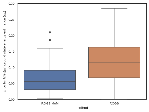
Figure 5: Advantage of the Median-of-means estimation for $\mathrm{NH_{3}}$ Using Jordan-Wigner [27] (JW) Encoding: This plot compares the ground state estimation results for the same molecule under the same settings when limited to 1000 total measurements, except that ROGS MoM employs the median-of-means estimator, highlighting its benefits. Here, we have set $K=M_{\ell}{\epsilon_{\ell}^{2}}/{\sigma_{\ell}^{2}}$, where $\epsilon_{\ell}=\epsilon/\sum_{\ell}|a_{\ell}|$, $\epsilon$ is the error bound as given by the confidence bound 1.

Appendix C Fine Graining Shots Allocation

In this section, we’ll discuss how to find the shots allocation in detail, specifically, how to determine the hyperparameter $\epsilon$ in (1) when we treat it as a convex optimization problem, which acts as the error bound of energy estimation of a particular state in (10). As observed in the confidence bound expression (1) in Theorem 1, the shot allocation, resulting from the minimization of the confidence bound, remains the same provided the product of the state energy estimation error bound and the total budget, $\epsilon^{2}M$, is kept constant. Assuming $\epsilon\leq\epsilon_{0}=2\sum_{\ell}|a_{\ell}|$ is valid for all states, we empirically choose $\epsilon=\epsilon_{0}(M_{0}/M)^{1/2}$ for a given budget $M$, for any $M_{0}\geq 0$, and determine the shot allocation by performing convex optimization on the confidence bound. This typically provides satisfactory results without necessitating the fine-tuning of the parameter $\epsilon$ for specific states, as delineated in Algorithm 3.3. By setting $M_{0}=1$, we can determine the fixed-shot outcomes for our ROGS method (see error table Table 3 ROGS Naive).

Molecule Encoding	$\mathrm{H_{2}}$ (-1.86)			$\mathrm{LiH}$ (-8.91)			$\mathrm{BeH_{2}}$ (-19.04)			$\mathrm{H_{2}O}$ (-83.6)			$\mathrm{NH_{3}}$ (-66.88)
	JW	P	BK	JW	P	BK	JW	P	BK	JW	P	BK	JW	P	BK
ROGS Naive	0.04	0.02	0.04	0.03	0.02	0.01	0.06	0.08	0.05	0.10	0.09	0.13	0.15	0.13	0.11
Even distribution	0.07	0.05	0.05	0.10	0.05	0.06	0.10	0.11	0.12	0.16	0.22	0.31	0.31	0.38	0.32

Table 3: Naive Estimation benchmark: This table shows the RMSE ($E_{h}$) of Naive shots distribution given by a fixed empirical error bound $\epsilon$ without pre-sampling (ROGS Naive), and the RMSE given by distributing the measurements evenly across all groups (Even distribution) by simulating the process 10 times, each with 1,000 measurements.

These results underscore the method’s robustness within a certain range of the parameter $\epsilon$. On the other hand, if one holds the product $\epsilon^{2}M$ fixed, the shots allocation ${w_{\alpha}}$ obtained by the convex optimization is fixed, and so is the confidence bound $\delta=\mathrm{Conf}\left[\epsilon_{0},{w_{\alpha}};M_{0},{\mathcal{H}}\right]$, which implies that this hyperparameter $\epsilon_{0}$ can be ascertained from a small number of measurements $M_{0}$. With $\epsilon_{0}^{2}M_{0}$ held fixed in  (1), the shot allocation $\{w_{\alpha}\}$ which minimizes the confidence bound is unchanged, meaning that if we increase the total number of shots to $M$ while setting $\epsilon=\epsilon_{0}\sqrt{M_{0}/M}$, the shots allocation $\{w^{\alpha}\}$ which minimizes the confidence bound $\delta=\mathrm{Conf}\left[\epsilon_{0},{w^{*}_{\alpha}};M_{0},{\mathcal{H}}\right]$ remains unchanged. Therefore, the algorithm can be improved by incorporating a coarse-grained search for the hyperparameter $\epsilon_{0}$ to find the minimum error of the energy estimation for a given state with a finite number of shot measurements $M_{0}$, where the energy estimation $\hat{\mathcal{H}}$ is obtained by quantum measurement using the measurement recipe $\{\mathcal{P}_{\alpha}^{\otimes M_{\alpha}^{0}}\}\in\{X,Y,Z\}^{n\times M_{0}},\leavevmode\nobreak\ (\sum M_{\alpha}^{0}=M)$, which is given by minimizing the confidence bound using a given $\epsilon_{0}$ following algorithm 3.3,

$$\mathrm{Error}(\{\{\mathcal{P}^{(m)}_{\alpha}\}_{1\leq m\leq M^{0}_{\alpha}}\})=\sqrt{\mathbb{E}\left[\left(\hat{{\mathcal{H}}}(\{\mathcal{P}_{\alpha}^{\otimes M_{\alpha}^{0}}\})-\langle{\mathcal{H}}\rangle_{\rho}\right)^{2}\right]};$$ (30)

then applying $\epsilon=\epsilon_{0}(M_{0}/M)^{1/2}$ for the total amount of shots $M$. Here is our detailed algorithm for determining the optimal shot allocation:

[H]

(Coarse-Graining Parameter ROGS)

1Measurement budget $M$ and Hamiltonian ${\mathcal{H}}=\sum_{\ell}a_{\ell}O_{\ell}$.

2A fixed Pauli basis measurement recipe $\{\mathcal{P}_{\alpha}^{\otimes M_{\alpha}}\}$ containing $\{X,Y,Z\}^{n\times M}$ for the classical shadow quantum measurement stage.

3Identify the max-min groups $\{C_{\alpha}^{\mathrm{MM}}\}$ of operators $\{O_{\ell}\}$ in ${\mathcal{H}}$ using Algorithm 3.1.

4initialize $error={}$

5while $i\leq N$ do $\triangleright$ Coarse-Graining with $M_{test}$ shots. Use $M_{cg}=M_{test}/N$ shots in each rounds

6    $M_{0}=random(0.1,10)$

7    $\epsilon_{cg}=2\sum_{\ell}|a_{\ell}|\sqrt{M_{0}/M_{cg}}$, total shots $=\leavevmode\nobreak\ M_{cg}$, run algorithm 3.3. Return recipe $\{\{\mathcal{P}^{(m)}_{\alpha}\}_{1\leq m\leq M_{\alpha}}\}$

8    $error[\epsilon_{cg}]=\mathrm{Error}(\{\mathcal{P}_{\alpha}^{\otimes M_{\alpha}^{cg}}\})$ (30)

9end while

10$\epsilon_{cg}^{*}=\min(error[\epsilon_{cg}]).key()$$\triangleright$ get optimal error rate for shots $M_{cg}$

11$\epsilon=\epsilon_{cg}\sqrt{M_{cg}/M}$ total shots $=\leavevmode\nobreak\ M$, run algorithm 3.3

Our algorithm shows a strong advantage after going through this process. One should note the hyperparameter $\epsilon$ in Theorem 1 influences the distribution of measurement shots among the groups. As $\epsilon$ decreases, the optimal shot allocation $w_{\alpha}$ tends to concentrate on the high-weight groups. Conversely, as $\epsilon$ increases, the shot distribution becomes more evenly spread across all groups. This behavior can be intuited from the role of $\epsilon$ in the confidence bound: a smaller $\epsilon$ demands higher precision, which is achieved by focusing measurements on the most significant terms in the Hamiltonian.

Interestingly, the cost function given by Section A.2 exhibits the opposite behavior when the weight factor $w_{\ell,\alpha}^{0}$ is concentrated on the high-weight groups. In this case, as the weight factors become more focused on the high-weight groups, the cost function tends to allocate shots more evenly among all groups. This is because the concentrated weight factors already prioritize the important terms, allowing the shot allocation to balance the measurement of less significant terms for overall accuracy. These contrasting behaviors highlight the interplay between the hyperparameter $\epsilon$, the weight factors $w_{\ell,\alpha}^{0}$, and the resulting shot allocation. The choice of $\epsilon$ and the definition of the weight factors should be carefully considered based on the desired balance between prioritizing important terms and ensuring a comprehensive measurement of the entire Hamiltonian. Further research into the optimal selection of these parameters for specific applications could lead to more efficient and effective measurement strategies in quantum algorithms.

References

- [1] John Preskill. “Quantum computing in the nisq era and beyond”. Quantum 2, 79 (2018).
- [2] M. Cerezo, Andrew Arrasmith, Ryan Babbush, Simon C. Benjamin, Suguru Endo, Keisuke Fujii, Jarrod R. McClean, Kosuke Mitarai, Xiao Yuan, Lukasz Cincio, and Patrick J. Coles. “Variational quantum algorithms”. Nature Reviews Physics 3, 625–644 (2021).
- [3] Kishor Bharti, Alba Cervera-Lierta, Thi Ha Kyaw, Tobias Haug, Sumner Alperin-Lea, Abhinav Anand, Matthias Degroote, Hermanni Heimonen, Jakob S. Kottmann, Tim Menke, Wai-Keong Mok, Sukin Sim, Leong-Chuan Kwek, and Alán Aspuru-Guzik. “Noisy intermediate-scale quantum algorithms”. Rev. Mod. Phys. 94, 015004 (2022).
- [4] Alberto Peruzzo, Jarrod McClean, Peter Shadbolt, Man-Hong Yung, Xiao-Qi Zhou, Peter J. Love, Alán Aspuru-Guzik, and Jeremy L. O’Brien. “A variational eigenvalue solver on a photonic quantum processor”. Nature Communications 5, 4213 (2014).
- [5] Jules Tilly, Hongxiang Chen, Shuxiang Cao, Dario Picozzi, Kanav Setia, Ying Li, Edward Grant, Leonard Wossnig, Ivan Rungger, George H. Booth, and Jonathan Tennyson. “The variational quantum eigensolver: A review of methods and best practices”. Physics Reports 986, 1–128 (2022).
- [6] Sergey B. Bravyi and Alexei Yu. Kitaev. “Fermionic quantum computation”. Annals of Physics 298, 210–226 (2002).
- [7] Jacob T. Seeley, Martin J. Richard, and Peter J. Love. “The bravyi-kitaev transformation for quantum computation of electronic structure”. The Journal of Chemical Physics 137, 224109 (2012).
- [8] Andrew Tranter, Peter J. Love, Florian Mintert, and Peter V. Coveney. “A comparison of the bravyi–kitaev and jordan–wigner transformations for the quantum simulation of quantum chemistry”. Journal of Chemical Theory and Computation 14, 5617–5630 (2018).
- [9] Vladyslav Verteletskyi, Tzu-Ching Yen, and Artur F. Izmaylov. “Measurement optimization in the variational quantum eigensolver using a minimum clique cover”. The Journal of Chemical Physics 152, 124114 (2020).
- [10] Tzu-Ching Yen, Vladyslav Verteletskyi, and Artur F. Izmaylov. “Measuring all compatible operators in one series of a single-qubit measurements using unitary transformations” (2020). arXiv:1907.09386.
- [11] Artur F Izmaylov, Tzu-Ching Yen, Robert A Lang, and Vladyslav Verteletskyi. “Unitary partitioning approach to the measurement problem in the variational quantum eigensolver method”. Journal of chemical theory and computation 16, 190–195 (2019).
- [12] Pranav Gokhale, Olivia Angiuli, Yongshan Ding, Kaiwen Gui, Teague Tomesh, Martin Suchara, Margaret Martonosi, and Frederic T. Chong. “Minimizing state preparations in variational quantum eigensolver by partitioning into commuting families” (2019). arXiv:1907.13623.
- [13] Richard M. Karp. “Reducibility among Combinatorial Problems”. In Raymond E. Miller, James W. Thatcher, and Jean D. Bohlinger, editors, Complexity of Computer Computations: Proceedings of a symposium on the Complexity of Computer Computations, held March 20–22, 1972, at the IBM Thomas J. Watson Research Center, Yorktown Heights, New York, and sponsored by the Office of Naval Research, Mathematics Program, IBM World Trade Corporation, and the IBM Research Mathematical Sciences Department. Pages 85–103. Springer US, Boston, MA (1972).
- [14] Hsin-Yuan Huang, Richard Kueng, and John Preskill. “Predicting many properties of a quantum system from very few measurements”. Nature Physics 16, 1050–1057 (2020).
- [15] Hsin-Yuan Huang, Richard Kueng, and John Preskill. “Efficient estimation of pauli observables by derandomization”. Phys. Rev. Lett. 127, 030503 (2021).
- [16] Charles Hadfield, Sergey Bravyi, Rudy Raymond, and Antonio Mezzacapo. “Measurements of quantum hamiltonians with locally-biased classical shadows” (2020). arXiv:2006.15788.
- [17] Charles Hadfield. “Adaptive pauli shadows for energy estimation” (2021). arXiv:2105.12207.
- [18] Alexander Gresch and Martin Kliesch. “Guaranteed efficient energy estimation of quantum many-body hamiltonians using shadowgrouping” (2023). arXiv:2301.03385.
- [19] Bujiao Wu, Jinzhao Sun, Qi Huang, and Xiao Yuan. “Overlapped grouping measurement: A unified framework for measuring quantum states”. Quantum 7, 896 (2023).
- [20] Ariel Shlosberg, Andrew J. Jena, Priyanka Mukhopadhyay, Jan F. Haase, Felix Leditzky, and Luca Dellantonio. “Adaptive estimation of quantum observables”. Quantum 7, 906 (2023).
- [21] Arkopal Dutt, William Kirby, Rudy Raymond, Charles Hadfield, Sarah Sheldon, Isaac L. Chuang, and Antonio Mezzacapo. “Practical benchmarking of randomized measurement methods for quantum chemistry hamiltonians” (2023). arXiv:2312.07497.
- [22] Almudena Carrera Vazquez, Caroline Tornow, Diego Riste, Stefan Woerner, Maika Takita, and Daniel J. Egger. “Scaling quantum computing with dynamic circuits” (2024). arXiv:2402.17833.
- [23] Caroline Tornow, Naoki Kanazawa, William E. Shanks, and Daniel J. Egger. “Minimum quantum run-time characterization and calibration via restless measurements with dynamic repetition rates”. Phys. Rev. Appl. 17, 064061 (2022).
- [24] Immanuel M. Bomze, Marco Budinich, Panos M. Pardalos, and Marcello Pelillo. “The maximum clique problem”. Pages 1–74. Springer US. Boston, MA (1999).
- [25] Ravi Boppana and Magnús M Halldórsson. “Approximating maximum independent sets by excluding subgraphs”. BIT Numerical Mathematics 32, 180–196 (1992).
- [26] Steven Diamond and Stephen Boyd. “Cvxpy: A python-embedded modeling language for convex optimization”. Journal of Machine Learning Research 17, 1–5 (2016). url: http://jmlr.org/papers/v17/15-408.html.
- [27] Pascual Jordan and Eugene Paul Wigner. “Über das paulische äquivalenzverbot”. Pages 109–129. Springer Berlin Heidelberg. Berlin, Heidelberg (1993).
- [28] Ali Javadi-Abhari, Matthew Treinish, Kevin Krsulich, Christopher J. Wood, Jake Lishman, Julien Gacon, Simon Martiel, Paul D. Nation, Lev S. Bishop, Andrew W. Cross, Blake R. Johnson, and Jay M. Gambetta. “Quantum computing with Qiskit” (2024). arXiv:2405.08810.
- [29] Pauli Virtanen, Ralf Gommers, Travis E. Oliphant, Matt Haberland, Tyler Reddy, David Cournapeau, Evgeni Burovski, Pearu Peterson, Warren Weckesser, Jonathan Bright, Stéfan J. van der Walt, Matthew Brett, Joshua Wilson, K. Jarrod Millman, Nikolay Mayorov, Andrew R. J. Nelson, Eric Jones, Robert Kern, Eric Larson, C J Carey, İlhan Polat, Yu Feng, Eric W. Moore, Jake VanderPlas, Denis Laxalde, Josef Perktold, Robert Cimrman, Ian Henriksen, E. A. Quintero, Charles R. Harris, Anne M. Archibald, Antônio H. Ribeiro, Fabian Pedregosa, Paul van Mulbregt, and SciPy 1.0 Contributors. “SciPy 1.0: Fundamental Algorithms for Scientific Computing in Python”. Nature Methods 17, 261–272 (2020).
- [30] Aric Hagberg, Pieter Swart, and Daniel S Chult. “Exploring network structure, dynamics, and function using networkx”. Technical report. Los Alamos National Lab.(LANL), Los Alamos, NM (United States) (2008). url: https://www.osti.gov/biblio/960616.
- [31] Ville Bergholm, Josh Izaac, Maria Schuld, Christian Gogolin, Shahnawaz Ahmed, Vishnu Ajith, M. Sohaib Alam, Guillermo Alonso-Linaje, B. AkashNarayanan, Ali Asadi, Juan Miguel Arrazola, Utkarsh Azad, Sam Banning, Carsten Blank, Thomas R Bromley, Benjamin A. Cordier, Jack Ceroni, Alain Delgado, Olivia Di Matteo, Amintor Dusko, Tanya Garg, Diego Guala, Anthony Hayes, Ryan Hill, Aroosa Ijaz, Theodor Isacsson, David Ittah, Soran Jahangiri, Prateek Jain, Edward Jiang, Ankit Khandelwal, Korbinian Kottmann, Robert A. Lang, Christina Lee, Thomas Loke, Angus Lowe, Keri McKiernan, Johannes Jakob Meyer, J. A. Montañez-Barrera, Romain Moyard, Zeyue Niu, Lee James O’Riordan, Steven Oud, Ashish Panigrahi, Chae-Yeun Park, Daniel Polatajko, Nicolás Quesada, Chase Roberts, Nahum Sá, Isidor Schoch, Borun Shi, Shuli Shu, Sukin Sim, Arshpreet Singh, Ingrid Strandberg, Jay Soni, Antal Száva, Slimane Thabet, Rodrigo A. Vargas-Hernández, Trevor Vincent, Nicola Vitucci, Maurice Weber, David Wierichs, Roeland Wiersema, Moritz Willmann, Vincent Wong, Shaoming Zhang, and Nathan Killoran. “Pennylane: Automatic differentiation of hybrid quantum-classical computations” (2018). arXiv:1811.04968.
- [32] Gareth James, Daniela Witten, Trevor Hastie, Robert Tibshirani, et al. “An introduction to statistical learning”. Volume 112. Springer. (2013).
- [33] Artur F Izmaylov, Tzu-Ching Yen, and Ilya G Ryabinkin. “Revising the measurement process in the variational quantum eigensolver: is it possible to reduce the number of separately measured operators?”. Chemical science 10, 3746–3755 (2019).
- [34] David Wierichs, Josh Izaac, Cody Wang, and Cedric Yen-Yu Lin. “General parameter-shift rules for quantum gradients”. Quantum 6, 677 (2022).
- [35] Tzu-Ching Yen, Aadithya Ganeshram, and Artur F Izmaylov. “Deterministic improvements of quantum measurements with grouping of compatible operators, non-local transformations, and covariance estimates”. npj Quantum Information 9, 14 (2023).