A Fast Single-Loop Primal-Dual Algorithm for Non-Convex Functional Constrained Optimization

Abstract

Non-convex functional constrained optimization problems have gained substantial attention in machine learning and signal processing. This paper develops a new primal-dual algorithm for solving this class of problems. The algorithm is based on a novel form of the Lagrangian function, termed Proximal-Perturbed Augmented Lagrangian, which enables us to develop an efficient and simple first-order algorithm that converges to a stationary solution under mild conditions. Our method has several key features of differentiation over existing augmented Lagrangian-based methods: (i) it is a single-loop algorithm that does not require the continuous adjustment of the penalty parameter to infinity; (ii) it can achieves an improved iteration complexity of $\widetilde{\mathcal{O}}(1/\epsilon^{2})$ or at least ${\mathcal{O}}(1/\epsilon^{2/q})$ with $q\in(2/3,1)$ for computing an $\epsilon$-approximate stationary solution, compared to the best-known complexity of $\mathcal{O}(1/\epsilon^{3})$; and (iii) it effectively handles functional constraints for feasibility guarantees with fixed parameters, without imposing boundedness assumptions on the dual iterates and the penalty parameters. We validate the effectiveness of our method through numerical experiments on popular non-convex problems.

I Introduction

We consider the following non-convex optimization problem with functional constraints:

$$\underset{\mathbf{x}\in\mathbb{R}^{n}}{\mathrm{min}}\ \ f(\mathbf{x})+r(\mathbf{x})\quad\mathrm{s.\>t.}\quad g(\mathbf{x})\leq\mathbf{0},$$ (1)

where $f:\mathbb{R}^{n}\rightarrow\mathbb{R}$ is a continuously differentiable and possibly non-convex function; $g:\mathbb{R}^{n}\rightarrow\mathbb{R}^{m}$ is a continuously differentiable and possibly non-convex mapping; and $r:\mathbb{R}^{n}\rightarrow\mathbb{R}\cup\{+\infty\}$ is a proper, closed, and convex (but possibly non-smooth) function.

Problems of the form (1) appear in a wide range of applications in signal processing and machine learning, e.g., wireless transmit/receive beamforming design [38, 40], and constrained classification/detection problems [17, 34, 47]. Solving non-convex problems, even those without constraints, is generally challenging, as finding even an approximate global minimum is often computationally intractable [30]. The presence of functional constraints $g(\mathbf{x})$ in (1) that can potentially be non-convex is critical for many of the applications mentioned above, yet it makes the problem even more challenging. A further complication arises since in many of these applications, problem (1) tends to be large-scale, i.e., with large variable dimension $n$ [10]. Hence, developing first-order methods that can find stationary solutions with lower complexity bounds is highly desirable.

Augmented Lagrangian (AL)-based algorithms are a prevailing class of approaches for constrained optimization problems. The foundational AL method, introduced by [16] and [33], has been a powerful algorithmic framework built on by many contemporary algorithms. In particular, the Alternating Direction Method of Multipliers (ADMM) scheme has been widely employed for solving constrained optimization problems based on the AL framework; see [3, 4] and recent works for constrained convex settings [31, 21, 45, 26, 46].

However, AL-based methods remain fairly limited for problems in the general form of (1) due to challenges posed by the non-convexity of the objective and constraint functions. Specifically, two major challenges arise: (i) difficulty in controlling the multipliers due to the absence of strong duality and, as a result, (ii) the need for careful updating of the penalty parameters to ensure the solution’s feasibility. Consequently, existing analyses of AL-based methods, with the best-known guarantees of $\mathcal{O}(1/\epsilon^{3})$ for a given $\epsilon>0$, require increasing penalty parameters to infinity to ensure feasibility, leading to higher iteration complexity. Effective handling of the multiplier sequence is thus an important and challenging task, given the increasing penalty parameters otherwise required for feasibility guarantees. Motivated by this, we aim to answer the question:

Can we design an algorithm to solve problems of the form (1) with an iteration complexity bound lower than the best-known result of $\mathcal{O}(1/\epsilon^{3})$?

TABLE I: Common boundedness and regularity assumptions of algorithms for non-convex constrained optimization problems.

Condition	Description
$\mathcal{B}$	Either $\text{dom}(r)$ is bounded and/or the feasible set is bounded.
$\mathcal{N}$	For every $\mathbf{x}\in\text{dom}(r)$, there exists $d>0$ such that $\partial r(\mathbf{x})\subseteq\mathcal{N}_{\text{dom}(r)}(\mathbf{x})+B_{d}(\mathbf{0})$, $B_{d}(\mathbf{0}):=\{\mathbf{x}:\|\mathbf{x}\|\leq d\}$.
$\mathcal{CO}$	Coercivity: the objective $f(\mathbf{x})$ is coercive, i.e., $\lim_{\|x\|\to\infty}f(\mathbf{x})=\infty$.
$\mathcal{RC}$	Regularity Condition: there is a constant $v>0$ such that $v\|[g(\mathbf{x}_{k})]^{+}\|\leq\text{dist}\left(\mathbf{0},\nabla g(\mathbf{x}_{k})[g(\mathbf{x}_{k})]^{+}+{\partial r(\mathbf{x}_{k})}/{\rho_{k-1}}\right)$
	for the generated sequence $\{\mathbf{x}_{k}\}$ and increasing sequence of penalty parameters $\{\rho_{k}\}$.
$\mathcal{SC}$	Slater’s Condition: there exists $\bar{\mathbf{x}}\in\text{int(dom}(r))$ such that $g(\bar{\mathbf{x}})<\mathbf{0}$.
$\mathcal{CQ}$	MFCQ: there exists $\mathbf{d}\in\mathbb{R}^{n}$ such that $\nabla g_{j}(\mathbf{x})^{\top}\mathbf{d}<0\ \text{for all }j\in J(\mathbf{x})=\{j\mid g_{j}(\mathbf{x})=0\}.$

TABLE II: Key properties of recent algorithms for solving non-convex constrained optimization problems compared with our method.

Algorithm	Constraints	Complexity	Simplicity	Key conditions
S-Prox ALM [49]	linear	$\mathcal{O}(1/\epsilon^{2})$	single-loop	$\mathcal{B,SC}$
NL-IAPIAL [18]	convex	$\widetilde{\mathcal{O}}(1/\epsilon^{3})$	double-loop	$\mathcal{B,N,SC}$
NOVA [37]	non-convex	unknown	double-loop	$\mathcal{CO,CQ}$
iALM [36]	non-convex	$\widetilde{\mathcal{O}}(1/\epsilon^{4})$	double-loop	$\mathcal{B,RC}$
iALM [23]	non-convex	$\widetilde{\mathcal{O}}(1/\epsilon^{3})$	double-loop	$\mathcal{B,RC}$
IPPP [25]	non-convex	$\widetilde{\mathcal{O}}(1/\epsilon^{3})$	triple-loop	$\mathcal{B,N,SC}$
GDPA [27]	non-convex	$\mathcal{O}(1/\epsilon^{3})$	single-loop	$\mathcal{B,RC}$
This paper	non-convex	${\boldsymbol{\widetilde{\mathcal{O}}(1/\epsilon^{2})}}$	single-loop	$\mathcal{B}$

To answer this question, we develop an efficient and easy-to-implement primal-dual method for solving problem (1) with an improved complexity result. In particular, for a given accuracy $\epsilon>0$, we propose a single-loop first-order method, based on a new augmented Lagrangian, to compute an $\epsilon$-approximate stationary solution (see Definition 2). We show that our method achieves an iteration complexity of $\widetilde{\mathcal{O}}(1/\epsilon^{2})$ in terms of the number of gradient evaluations.

I-A Related Work

We review the literature on iteration complexity and convergence of AL and penalty-based methods for non-convex constrained problems. To facilitate the discussion, Table I summarizes key assumptions imposed by existing algorithms. Table II differentiates our work from several key existing papers, comparing the constraint types handled, iteration complexities, algorithmic simplicity, and necessary conditions from Table I.

Linearly constrained non-convex problems. Many existing works have focused on the class of problems where $g(\mathbf{x})$ in (1) is linear. [15] introduced a perturbed-proximal primal-dual algorithm, with an iteration complexity of $\widetilde{\mathcal{O}}(1/\epsilon^{4})$, under the assumption of a feasible initialization. [19] proposed proximal AL methods that obtain the improved complexity result of $\widetilde{\mathcal{O}}(1/\epsilon^{3})$ under Slater’s condition. Finally, [48, 49] proposed a first-order single-loop proximal AL method that achieves $\mathcal{O}(1/\epsilon^{2})$ iteration complexity, which relies on error bounds that are dependent on the Hoffman constant of the polyhedral constraints. However, estimating the Hoffman constant is known to be difficult in practice.

Non-convex functional constrained problems. There are several recent works that focus on the iteration complexity of first-order AL-based methods or penalty methods to solve (1) [11, 37, 23, 25, 27, 18, 36]. [37] proposed double-loop distributed primal-dual algorithms with asymptotic convergence guarantees, under the coercivity assumption and Mangasarian-Fromovitz constraint qualification (MFCQ). However, it has been observed that many non-convex problems do not have a strict relative interior, and thus have an unbounded set of multipliers [14], which violates MFCQ. More recently, a set of methods have emerged employing the regularity condition ($\mathcal{RC}$) from Table I for ensuring solution feasibility. [36] proposed a double-loop inexact AL method (iALM) that achieves an $\widetilde{\mathcal{O}}(1/\epsilon^{4})$ iteration complexity. [23] improved the iteration complexity to $\widetilde{\mathcal{O}}(1/\epsilon^{3})$, which is obtained using a triple loop iALM. [18] established an $\widetilde{\mathcal{O}}(1/\epsilon^{3})$ complexity bound of the proximal AL method (NL-IAPIAL) for non-convex problems with nonlinear convex constraints. [27] proposed the first single-loop gradient-based algorithm that achieves the best-known iteration complexity $\mathcal{O}(1/\epsilon^{3})$ for (1). However, the regularity condition is non-standard and rather strong as it forces a relationship between feasibility of the generated iterates and first-order optimality. We are thus motivated to develop an algorithm that improves iteration complexity without requiring this assumption.

I-B Our Contributions

We develop a novel AL-based method for solving non-convex constrained optimization problems which has improved iteration complexity, computation workload, and weaker assumption requirements. Specifically:

• We propose a single-loop first-order algorithm for non-convex optimization problems with functional constraints, based on a novel Lagrangian function. The proposed algorithm can achieves an $\epsilon$-KKT solution with $\widetilde{\mathcal{O}}(1/\epsilon^{2})$ iteration complexity, which improves the best-known $\mathcal{O}(1/\epsilon^{3})$ complexity for the functionally constrained non-convex setting. Importantly, the algorithm does not require the strong regularity condition used in other AL-based algorithms [23, 25, 27, 36].

• To establish the above results, we conduct a comprehensive convergence analysis of our method. Thanks to the favorable structure of our Lagrangian, our proofs are surprisingly compact compared to existing works. Our analysis does not impose any boundedness assumptions on the multiplier sequence, surjectivity of the Jacobian $\nabla g(\mathbf{x})$ [6, 9], or boundedness of penalty parameters [13]. It also does not require the feasibility of initialization as in [7, 42, 44].

• By using a fixed penalty parameter, our algorithm achieves improved computational efficiency and ease of implementation compared to existing schemes. Specifically, we neither require linear independence constraint qualification (LICQ) to ensure boundedness of penalty parameters [41], nor computational efforts for careful updating scheme of the penalty parameters. Our numerical results validate that compared with existing methods, our use of a fixed penalty parameter achieves more consistent progress toward solution stationarity and feasibility.

I-C Outline

Section II provides the notation, definitions, and assumptions that we use throughout the paper. In Section III, we introduce the new Lagrangian and propose a first-order primal-dual algorithm. In Section IV, we establish the convergence results of our algorithm. Section V presents numerical results on commonly encountered problems in signal processing and machine learning to demonstrate the effectiveness of the proposed algorithm.

II Preliminaries

We provide some notation used throughout the paper. Let $\mathbb{R}^{n}$ and $\mathbb{R}^{n}_{+}$ denote the $n$-dimensional Euclidean space and the non-negative orthant, respectively. We let $[m]$ denote the set $\{1,\ldots,m\}$. The vector inner product is denoted by $\left\langle\cdot,\cdot\right\rangle$. The Euclidean norm of matrices and vectors are denoted by $\left\|\>\cdot\>\right\|$. The distance function between a vector $\mathbf{x}$ and a set $\mathcal{X}\subseteq\mathbb{R}^{n}$ is defined by $\text{dist}(\mathbf{x},\mathcal{X}):=\inf_{\mathbf{y}\in\mathcal{X}}\|\mathbf{y}-\mathbf{x}\|.$ The domain of a proper extended real-valued function $r$ is defined by $\textrm{dom}(r):=\left\{\mathbf{x}\in\mathbb{R}^{n}:r(\mathbf{x})<+\infty\right\}.$ The subgradient of a convex function $r$ at $\mathbf{x}$ is denoted by $\partial r(\mathbf{x}):=\left\{\mathbf{d}\in\mathbb{R}^{n}:r(\mathbf{y})\geq r(\mathbf{x})+\left\langle\mathbf{d},\mathbf{y}-\mathbf{x}\right\rangle,\forall\mathbf{y}\in\mathbb{R}^{n},\ \mathbf{x}\in\text{dom}(r)\right\}.$ We say a function $r$ is proper if $\text{dom}(r)\neq\emptyset$ and it does not take the value $-\infty$. The function $r$ is called closed if it is lower semicontinuous, i.e., $\liminf_{\mathbf{x}\rightarrow\mathbf{x}^{0}}r(\mathbf{x})\geq r(\mathbf{x}^{0})$ for any $\mathbf{x}^{0}\in\mathbb{R}^{n}$. Given a proper, closed, and convex function $r:\mathbb{R}^{n}\rightarrow\mathbb{R}\cup\left\{+\infty\right\}$, $\mathbf{x}\in\mathbb{R}^{n}$ and $\eta>0$, the proximal map associated with $r$ is uniquely defined by $\text{prox}_{\eta r}(\mathbf{x})={\text{argmin}_{\mathbf{y}\in\mathbb{R}^{n}}}\left\{r(\mathbf{y})+\frac{1}{2\eta}\|\mathbf{x}-\mathbf{y}\|^{2}\right\}.$

Next, we provide the formal definitions and assumptions for the class of functions, and the optimality measure under consideration. Assuming that a suitable constraint qualification (CQ) hold, the stationary solutions of problem (1) can be characterized by the points $(\mathbf{x}^{\ast},\boldsymbol{\lambda}^{\ast})$ satisfying the Karush-Kuhn-Tucker (KKT) conditions [2]:

Definition 1 (The KKT point).

A point $\mathbf{x}^{\ast}$ is called a KKT point for problem (1) if there exists $\boldsymbol{\lambda}^{\ast}\in\mathbb{R}^{m}$ such that

$$\begin{cases}\mathbf{0}\in\nabla f(\mathbf{x}^{\ast})+\partial r(\mathbf{x}^{\ast})+\langle\nabla g(\mathbf{x}^{\ast}),\boldsymbol{\lambda}^{\ast}\rangle,\\ \boldsymbol{\lambda}_{j}^{\ast}\geq 0,\ \ g_{j}(\mathbf{x}^{\ast})\leq 0,\ \ \boldsymbol{\lambda}_{j}g_{j}(\mathbf{x}^{\ast})=0,\ \ j\in[m].\end{cases}$$ (2)

A suitable CQ is necessary for the existence of multipliers that satisfy the KKT conditions (e.g., MFCQ, CPLD, and others; see [1]). In practice, it is difficult to find an exact KKT solution $(\mathbf{x}^{\ast},\boldsymbol{\lambda}^{\ast})$ that satisfies (2). We are thus interested in finding an approximate KKT solution defined as $\epsilon$-KKT solution of problem (1):

Definition 2 ($\epsilon$-KKT solution).

Given $\epsilon>0$, a point $\mathbf{x}^{\star}$ is called an $\epsilon$-KKT solution for problem (1) if there exists $\boldsymbol{\lambda}^{\star}\in\mathbb{R}^{m}_{+}$ such that

$$\begin{cases}\mathbf{v}^{\star}\in\nabla f(\mathbf{x}^{\star})+\partial r(\mathbf{x}^{\star})+\nabla g(\mathbf{x}^{\star})\boldsymbol{\lambda}^{\star},\quad\|\mathbf{v}^{\star}\|\leq\epsilon,\\ \|\max\{0,g(\mathbf{x}^{\star})\}\|\leq\epsilon,\quad\left\langle\boldsymbol{\lambda},g(\mathbf{x}^{\star})\right\rangle\leq\epsilon,\end{cases}$$

where $\max\{\mathbf{0},g(\mathbf{x}^{\star})\}$ denotes the component-wise maximum of $g(\mathbf{x}^{\star})$ and the zero vector $\mathbf{0}$ at $\mathbf{x}^{\star}$.

We make the following assumptions on problem (1).

Assumption 3.

There exists a point $(\mathbf{x},\boldsymbol{\lambda})\in\text{dom}(r)\times\mathbb{R}^{m}$ satisfying the KKT conditions (2).

Assumption 4.

$\nabla f$ and $\nabla g$ are $L_{f}$-Lipschitz continuous and $L_{g}$-Lipschitz continuous on $\text{dom}(r)$, respectively. That is, there exist $L_{f},L_{g}>0$ such that

$$\|\nabla f(\mathbf{x})-\nabla f(\mathbf{x}^{\prime})\| \leq L_{f}\|\mathbf{x}-\mathbf{x}^{\prime}\|,\ \forall\mathbf{x},\mathbf{x}^{\prime}\in\text{dom}(r),$$

$$\|\nabla g(\mathbf{x})-\nabla g(\mathbf{x}^{\prime})\| \leq L_{g}\|\mathbf{x}-\mathbf{x}^{\prime}\|,\ \forall\mathbf{x},\mathbf{x}^{\prime}\in\text{dom}(r).$$

Assumption 5.

The domain of $r$ is compact, i.e., $D_{\mathbf{x}}:={\max}_{\mathbf{x},\mathbf{x}^{\prime}\in\text{dom}(r)}\|\mathbf{x}-\mathbf{x}^{\prime}\|<+\infty.$

The assumptions above are quite standard and are satisfied by a wide range of practical problems in signal processing and machine learning [6, 24, 23, 27, 18, 28]. In this work, we do not make some restrictive assumptions found in prior work, including the surjectivity of $\nabla g(\mathbf{x})$ (or that $\nabla g(\mathbf{x})\nabla g(\mathbf{x})^{\top}$ is positive definite) [6, 8, 9, 22], feasibility of the initialization [7, 15, 44], and Slater’s condition [7, 18]. Note that many problems with an unbounded $\text{dom}(r)$ can be reformulated as problems satisfying Assumption 5. Specifically, as long as $f$ is bounded below and $r$ is coercive, the problem can be reformulated as a problem with $f+r$ for some $r$ (e.g., norm functions) with a compact domain [28].

We also note that under Assumption 5, there exist constants $B_{g}>0$ and $M_{g}>0$ such that

$$\underset{\mathbf{x}\in\text{dom}(r)}{\max}\|g(\mathbf{x})\|\leq B_{g}\ \ \text{and}\ \ \underset{\mathbf{x}\in\text{dom}(r)}{\max}\|\nabla g(\mathbf{x})\|\leq M_{g},$$ (3)

which implies Lipschitz continuity of $g$ [35, Chapter 9.B], i.e., $\|g(\mathbf{x})-g(\mathbf{x}^{\prime})\|\leq M_{g}\|\mathbf{x}-\mathbf{x}^{\prime}\|,\ \ \forall\mathbf{x},\mathbf{x}^{\prime}\in\text{dom}(r).$

III Proximal-Perturbed Augmented
Lagrangian Algorithm

In this section, we present our novel form of augmented Lagrangian (Section III-A) and propose a single-loop primal-dual algorithm based on it (Section III-B).

III-A Proximal-Perturbed Augmented Lagrangian

We first recast problem (1) as an equivalent equality-constrained problem using slack variables $\mathbf{u}\in\mathbb{R}^{m}_{+}$ [2]:

$$\underset{\mathbf{x}\in\mathbb{R}^{n},\mathbf{u}\in\mathbb{R}^{m}_{+}}{\mathrm{min}}\ f(\mathbf{x})+r(\mathbf{x})\quad\mathrm{s.\>t.}\quad g(\mathbf{x})+\mathbf{u}=\mathbf{0}.$$ (4)

By employing perturbation variables $\mathbf{z}\in\mathbb{R}^{m}$ and letting $g(\mathbf{x})+\mathbf{u}=\mathbf{z}$ and $\mathbf{z}=\mathbf{0}$, we then transform problem (4) into an extended formulation:

$$\underset{\mathbf{x}\in\mathbb{R}^{n},\mathbf{u}\in\mathbb{R}^{m}_{+},\mathbf{z}\in\mathbb{R}^{m}}{\mathrm{min}}f(\mathbf{x})+r(\mathbf{x})\ \ \mathrm{s.\>t.}\ \ g(\mathbf{x})+\mathbf{u}=\mathbf{z},\ \ \mathbf{z}=\mathbf{0}.$$

The equivalence of the extended formulation with problem (4) is obvious for the unique solution $\mathbf{z}^{\ast}=\mathbf{0}$. Now we define the Proximal-Perturbed Augmented Lagrangian (PPAL):

$$\mathcal{L}_{\rho}(\mathbf{x},\mathbf{u},\mathbf{z},\boldsymbol{\lambda},\boldsymbol{\mu})=\ell_{\rho}(\mathbf{x},\mathbf{u},\mathbf{z},\boldsymbol{\lambda},\boldsymbol{\mu})+r(\mathbf{x}),$$ (5)

where

$$\ell_{\rho}(\cdot) :=f(\mathbf{x})+\left\langle\boldsymbol{\lambda},g(\mathbf{x})+\mathbf{u}-\mathbf{z}\right\rangle+\left\langle\boldsymbol{\mu},\mathbf{z}\right\rangle+\frac{\alpha}{2}\|\mathbf{z}\|^{2}$$

$$\qquad-\frac{\beta}{2}\|\boldsymbol{\lambda}-\boldsymbol{\mu}\|^{2}+\frac{\rho}{2}\|g(\mathbf{x})+\mathbf{u}\|^{2}.$$ (6)

Here, $\boldsymbol{\lambda}\in\mathbb{R}^{m}$ is the multiplier (dual) associated with the functional constraint $g(\mathbf{x})+\mathbf{u}-\mathbf{z}=\mathbf{0}$ and $\boldsymbol{\mu}\in\mathbb{R}^{m}$ is the (auxiliary) multiplier associated with the additional constraint $\mathbf{z}=\mathbf{0}$. $\alpha>0$ is a penalty parameter, $\beta>0$ is a dual proximal parameter, and $\rho>0$ is a penalty parameter set to $\rho:=\frac{\alpha}{1+\alpha\beta}$.

The PPAL function, $\mathcal{L}_{\rho}(\mathbf{x},\mathbf{u},\mathbf{z},\boldsymbol{\lambda},\boldsymbol{\mu})$, presents a favorable structure for the development of efficient algorithms to solve non-convex constrained optimization problems. Its structure differentiates it from the standard AL function and its variants as described in e.g., [3, 4] and references therein. Specifically, note the additional constraint $\mathbf{z}=\mathbf{0}$ is penalized with the quadratic term $\frac{\alpha}{2}\|\mathbf{z}\|^{2}$, and the negative quadratic term $-\frac{\beta}{2}\|\boldsymbol{\lambda}-\boldsymbol{\mu}\|^{2}$ is added to the Lagrangian. To see the reasoning here, observe that if we minimize $\left\{-\left\langle\boldsymbol{\lambda}-\boldsymbol{\mu},\mathbf{z}\right\rangle+\frac{\alpha}{2}\|\mathbf{z}\|^{2}\right\}$ with respect to $\mathbf{z}$ for given $(\boldsymbol{\lambda},\boldsymbol{\mu})$, we have

$$-(\boldsymbol{\lambda}-\mu)+\alpha\mathbf{z}=\mathbf{0}\ \ \Longrightarrow\ \ \mathbf{z}(\boldsymbol{\lambda},\boldsymbol{\mu})=(\boldsymbol{\lambda}-\boldsymbol{\mu})/{\alpha},$$ (7)

which implies $\boldsymbol{\lambda}=\boldsymbol{\mu}$ at the solution $\mathbf{z}^{\ast}=\mathbf{0}$. Based on the relation between $\boldsymbol{\lambda}$ and $\boldsymbol{\mu}$ at $\mathbf{z}^{\ast}=\mathbf{0}$, a proximal dual regularization term $-\frac{\beta}{2}\|\boldsymbol{\lambda}-\boldsymbol{\mu}\|^{2}$ was incorporated, to make the Lagrangian smooth and strongly concave in $\boldsymbol{\lambda}$ for fixed $\boldsymbol{\mu}$ and in $\boldsymbol{\mu}$ for fixed $\boldsymbol{\lambda}$. This strong concavity enables us to design an efficient and stable dual update scheme in Section III-B. Substituting $\mathbf{z}(\boldsymbol{\lambda},\boldsymbol{\mu})$ into $\mathcal{L}_{\rho}(\mathbf{x},\mathbf{u},\mathbf{z},\boldsymbol{\lambda},\boldsymbol{\mu})$ yields the following reduced PPAL:

$$\mathcal{L}_{\rho}(\mathbf{x},\mathbf{u},\mathbf{z}(\boldsymbol{\lambda},\boldsymbol{\mu}),\boldsymbol{\lambda},\boldsymbol{\mu}) =f(\mathbf{x})+\left\langle\boldsymbol{\lambda},g(\mathbf{x})+\mathbf{u}\right\rangle-\frac{1}{2\rho}\|\boldsymbol{\lambda}-\boldsymbol{\mu}\|^{2}$$

$$\quad+\frac{\rho}{2}\|g(\mathbf{x})+\mathbf{u}\|^{2}+r(\mathbf{x}).$$ (8)

Note that $\mathcal{L}_{\rho}(\mathbf{x},\mathbf{u},\mathbf{z}(\boldsymbol{\lambda},\boldsymbol{\mu}),\boldsymbol{\lambda},\boldsymbol{\mu})$ is $\frac{1}{\rho}$-strongly concave in $\boldsymbol{\lambda}$ and hence there exists a unique maximizer $\boldsymbol{\lambda}(\mathbf{x},\boldsymbol{\mu})$. Maximizing $\mathcal{L}_{\rho}(\mathbf{x},\mathbf{u},\mathbf{z}(\boldsymbol{\lambda},\boldsymbol{\mu}),\boldsymbol{\lambda},\boldsymbol{\mu})$ with respect to $\boldsymbol{\lambda}$, we obtain

$$\boldsymbol{\lambda}(\mathbf{x},\boldsymbol{\mu}) =\underset{\boldsymbol{\lambda}\in\mathbb{R}^{m}}{\textrm{argmax}}\;\mathcal{L}_{\rho}(\mathbf{x},\mathbf{u},\mathbf{z}(\boldsymbol{\lambda},\boldsymbol{\mu}),\boldsymbol{\lambda},\boldsymbol{\mu})$$

$$=\boldsymbol{\mu}+\rho(g(\mathbf{x})+\mathbf{u}),$$ (9)

which will be used for the update of $\boldsymbol{\lambda}$ in (13).

III-B Description of Algorithm

We propose a single-loop first-order algorithm based on the properties of our PPAL that computes a stationary solution to the problem (1). At each iteration, the algorithm first updates $\mathbf{x}$ inexactly by

$$\mathbf{x}_{k+1} =\underset{\mathbf{x}\in\mathbb{R}^{n}}{\mathrm{argmin}}\left\{\left\langle\nabla_{\mathbf{x}}\ell_{\rho}(\mathbf{x}_{k},\mathbf{z}_{k},\boldsymbol{\lambda}_{k},\boldsymbol{\mu}_{k}),\mathbf{x}-\mathbf{x}_{k}\right\rangle\right.$$

$$\hskip 50.58878pt\left.+(1/{2\eta})\|\mathbf{x}-\mathbf{x}_{k}\|^{2}+r(\mathbf{x})\right\},$$

which is known as the proximal gradient mapping (see e.g., [5]) and can be rewritten as

$$\mathbf{x}_{k+1}=\text{prox}_{\eta r}\left[\mathbf{x}_{k}-\eta\nabla_{\mathbf{x}}\ell_{\rho}(\mathbf{x}_{k},\mathbf{u}_{k},\mathbf{z}_{k},\boldsymbol{\lambda}_{k},\boldsymbol{\mu}_{k})\right].$$

Algorithm 1 PPAL-based first-order Algorithm (PPALA)

1:  Input: Initialization $(\mathbf{x}_{0},\mathbf{u}_{0},\mathbf{z}_{0},\boldsymbol{\lambda}_{0},\boldsymbol{\mu}_{0})$, and parameters $\alpha>1$, $\beta\in(0,1)$, $\rho=\frac{\alpha}{1+\alpha\beta}$, and $K$.

2:  for $k=0,1,\dots,K$ do

3:      Compute $\mathbf{x}_{k+1}$ by the proximal gradient scheme:

$$\mathbf{x}_{k+1} =\underset{\mathbf{x}\in\mathbb{R}^{n}}{\mathrm{argmin}}\left\{\left\langle\nabla_{\mathbf{x}}\ell_{\rho}(\mathbf{x}_{k},\mathbf{u}_{k},\mathbf{z}_{k},\boldsymbol{\lambda}_{k},\boldsymbol{\mu}_{k}),\mathbf{x}-\mathbf{x}_{k}\right\rangle\right.$$

$$\hskip 50.58878pt\left.+({1}/{2\eta})\|\mathbf{x}-\mathbf{x}_{k}\|^{2}+r(\mathbf{x})\right\};$$ (10)

4:      Compute $\mathbf{u}_{k+1}$ by the projected gradient descent:

$$\mathbf{u}_{k+1}=\Pi_{[0,U]}[\mathbf{u}_{k}-\tau(\boldsymbol{\lambda}_{k}+\rho(g(\mathbf{x}_{k+1})+\mathbf{u}_{k})];$$ (11)

5:      Update the auxiliary multiplier $\boldsymbol{\mu}_{k+1}$ by:

$$\boldsymbol{\mu}_{k+1} =\boldsymbol{\mu}_{k}+\sigma_{k}(\boldsymbol{\lambda}_{k}-\boldsymbol{\mu}_{k}),\ \sigma_{k}=\frac{\delta_{k}}{\|\boldsymbol{\lambda}_{k}-\boldsymbol{\mu}_{k}\|^{2}+1};$$ (12)

6:      Update the multiplier $\boldsymbol{\lambda}_{k+1}$ by

$$\boldsymbol{\lambda}_{k+1}=\boldsymbol{\mu}_{k+1}+\rho(g(\mathbf{x}_{k+1})+\mathbf{u}_{k+1});$$ (13)

7:      Compute $\mathbf{z}_{k+1}$ by

$$\mathbf{z}_{k+1}=\frac{1}{\alpha}(\boldsymbol{\lambda}_{k+1}-\boldsymbol{\mu}_{k+1});$$ (14)

8:  end for

The next step is to update slack variable $\mathbf{u}$ using a projected gradient descent on $\mathcal{L}_{\rho}$:

$$\mathbf{u}_{k+1} =\Pi_{[0,U]}[\mathbf{u}_{k}-\tau(\nabla_{\mathbf{u}}\mathcal{L}_{\rho}(\mathbf{x}_{k},\mathbf{u}_{k},\mathbf{z}_{k},\boldsymbol{\lambda}_{k},\boldsymbol{\mu}_{k})]$$

$$=\Pi_{[0,U]}[\mathbf{u}_{k}-\tau(\boldsymbol{\lambda}_{k}+\rho(g(\mathbf{x}_{k+1})+\mathbf{u}_{k})],$$

where $\Pi_{[0,U]}(\mathbf{u}):=\textrm{argmin}\left\{\left\|\mathbf{u}-\mathbf{v}\right\|\left|\right.\mathbf{v}\in[0,U]\right\}$ denotes the projection of $\mathbf{u}$ onto the set $[0,U]$. Note that, without loss of generality, we can construct an upper bound $U:=B_{g}$ on $\mathbf{u}_{k+1}\in\mathbb{R}^{m}_{+}$ from (3) since we have $\|g(\mathbf{x})\|\leq B_{g}$ for all feasible solutions $\mathbf{x}$.

Next, the auxiliary multiplier $\boldsymbol{\mu}$ is updated as

$$\boldsymbol{\mu}_{k+1}=\boldsymbol{\mu}_{k}+\sigma_{k}(\boldsymbol{\lambda}_{k}-\boldsymbol{\mu}_{k}).$$

Here, the step size $\sigma_{k}>0$ is defined by $\sigma_{k}=\frac{\delta_{k}}{\|\boldsymbol{\lambda}_{k}-\boldsymbol{\mu}_{k}\|^{2}+1}$ in which $\delta_{k}$ is a diminishing sequence satisfying the conditions:

$$\delta_{0}\in(0,1],\ \ \lim_{k\to\infty}\delta_{k}=0,\ \ \text{and}\ \ \sum_{k=0}^{\infty}\delta_{k}=+\infty.$$ (15)

In particular, we employ the following sequence in our algorithm for which the conditions in (15) hold:

$$\delta_{k}=\frac{1}{p\cdot k^{q}+1},\quad\ \frac{2}{3}<q\leq 1,$$ (16)

where $p$ is a positive constant. Note that several alternatives are available for the sequence $\{\delta_{k}\}$ satisfying the conditions in (15). Two popular alternative step sizes are: (i) $\delta_{k}=\frac{\delta_{0}}{(k+1)^{q}}$, where $\delta_{0}>0$ and $0<q\leq 1$, and (ii) $\delta_{k}=\frac{\delta_{k-1}}{1-b\delta_{k-1}}$, where $\delta_{0}\in(0,1]$ and $b\in(0,1)$; see e.g., [2, 39] for more possibilities for $\{\delta_{k}\}$. As we will see in Theorem 11 and Corollary 12, a benefit of (16) and choosing $q\in(2/3,1]$ is that it allows our algorithm to achieve improved complexity bounds compared to $\mathcal{O}(1/\epsilon^{3})$ found in existing works (see Table II).

With updated ($\mathbf{x}_{k+1},\mathbf{u}_{k+1},\boldsymbol{\mu}_{k+1}$), the multiplier $\boldsymbol{\lambda}$ is then updated using (9):

$$\boldsymbol{\lambda}_{k+1} =\boldsymbol{\mu}_{k+1}+\rho(g(\mathbf{x}_{k+1})+\mathbf{u}_{k+1}).$$

The last step is to update $\mathbf{z}$ via an exact minimization scheme on $\mathcal{L}_{\rho}$ for the updated $(\boldsymbol{\lambda}_{k+1},\boldsymbol{\mu}_{k+1})$ with fixed parameter $\alpha>0$ based on (7):

$$\mathbf{z}_{k+1} =\underset{\mathbf{z}\in\mathbb{R}^{m}}{\mathrm{argmin}}\left\{\mathcal{L}_{\rho}(\mathbf{x}_{k+1},\mathbf{u}_{k+1},\mathbf{z},\boldsymbol{\lambda}_{k+1},\boldsymbol{\mu}_{k+1})\right\}$$

$$={(\boldsymbol{\lambda}_{k+1}-\boldsymbol{\mu}_{k+1})}/{\alpha}.$$

The steps of our proposed algorithm are summarized in Algorithm 1.

IV Convergence Analysis

In this section, we establish the convergence results of Algorithm 1. We prove that the sequence generated by Algorithm 1 converges to a KKT point as defined in (2). A roadmap of our analysis is as follows:

1. First, we provide important relations on the sequences $\{\boldsymbol{\lambda}_{k}\}$, $\{\boldsymbol{\mu}_{k}\}$, and $\{\mathbf{x}_{k}\}$ (Lemma 6) as well as the boundedness of multipliers $\{\boldsymbol{\lambda}_{k}\}$ and $\{\boldsymbol{\mu}_{k}\}$ (Lemma 7), directly derived from the structure of our algorithm. We also show the Lipschitz continuity of $\nabla_{\mathbf{x}}\ell_{\rho}$ (Lemma 8).

2. The above results are exploited to show that the sequence $\{\mathcal{L}_{\rho}\}$ is approximately decreasing and convergent (Lemma 9). Then, using the error bound for the subgradient of $\mathcal{L}_{\rho}$ (Lemma 10), together with Lemma 9, we prove the convergence of primal sequences $\{\mathbf{x}_{k}\}$ and $\{\mathbf{u}_{k}\}$ to some finite values satisfying stationarity in the KKT conditions (Theorem 11).

3. By building on the above results and utilizing the definitions of $\boldsymbol{\lambda}_{k+1}$ and $\boldsymbol{\mu}_{k+1}$, we readily establish the feasibility guarantees (Theorem 14).

IV-A Intermediate Inequalities and Bounds

We first provide basic yet crucial relations on the sequences $\{\boldsymbol{\lambda}_{k}\}$, $\{\boldsymbol{\mu}_{k}\}$, and $\{\mathbf{x}_{k}\}$.

Lemma 6.

Under Assumption 5, let $\{(\mathbf{x}_{k},\mathbf{u}_{k},\mathbf{z}_{k},\boldsymbol{\lambda}_{k},\boldsymbol{\mu}_{k})\}$ be the sequence generated by Algorithm 1 with the choice of the sequence $\{\delta_{k}\}$ as in (16). Then, for any $k\geq 1$,

$$\|\boldsymbol{\mu}_{k+1}-\boldsymbol{\mu}_{k}\|^{2} =\sigma_{k}^{2}\|\boldsymbol{\lambda}_{k}-\boldsymbol{\mu}_{k}\|^{2}\leq{\delta_{k}^{2}}/{4},$$ (17)

$$\sigma_{k}\|\boldsymbol{\lambda}_{k}-\boldsymbol{\mu}_{k}\|^{2} \leq\delta_{k},$$ (18)

$$\|\boldsymbol{\mu}_{k+1}-\boldsymbol{\lambda}_{k}\|^{2} =(1-\sigma_{k})^{2}\|\boldsymbol{\lambda}_{k}-\boldsymbol{\mu}_{k}\|^{2},$$ (19)

$$\|\boldsymbol{\lambda}_{k+1}-\boldsymbol{\lambda}_{k}\|^{2} \leq 3\rho^{2}M_{g}^{2}\|\mathbf{x}_{k+1}-\mathbf{x}_{k}\|^{2}$$

$$\quad+3\rho^{2}\|\mathbf{u}_{k+1}-\mathbf{u}_{k}\|^{2}+{3\delta_{k}^{2}}/{4}.$$ (20)

where $M_{g}$ denotes the Lipschitz constant of $g$ from (3).

Proof.

From the $\boldsymbol{\mu}$-update and noting that ${a}+{b}\geq 2\sqrt{{ab}}$ for any ${a,b}\geq 0$, we obtain the relations in (17):

$$\|\boldsymbol{\mu}_{k+1}-\boldsymbol{\mu}_{k}\|^{2} =\sigma_{k}^{2}\|\boldsymbol{\lambda}_{k}-\boldsymbol{\mu}_{k}\|^{2}$$

$$=\frac{\delta_{k}^{2}}{\|\boldsymbol{\lambda}_{k}-\boldsymbol{\mu}_{k}\|^{2}+2+\frac{1}{\|\boldsymbol{\lambda}_{k}-\boldsymbol{\mu}_{k}\|^{2}}}\leq\frac{\delta_{k}^{2}}{4}.$$

By the definitions $\sigma_{k}=\frac{\delta_{k}}{\|\boldsymbol{\lambda}_{k}-\boldsymbol{\mu}_{k}\|^{2}+1}\leq 1$ and $\delta_{k}\in(0,1]$, we know that $\sigma_{k}\leq 1$. Thus, we obtain the relation (18):

$$\sigma_{k}\|\boldsymbol{\lambda}_{k}-\boldsymbol{\mu}_{k}\|^{2}=\frac{\delta_{k}}{1+\frac{1}{\|\boldsymbol{\lambda}_{k}-\boldsymbol{\mu}_{k}\|^{2}}}\leq\delta_{k}.$$

Subtracting $\boldsymbol{\mu}_{k+1}$ from $\boldsymbol{\lambda}_{k}$ yields

$$\|\boldsymbol{\lambda}_{k}-\boldsymbol{\mu}_{k+1}\|=\|\boldsymbol{\lambda}_{k}-\boldsymbol{\mu}_{k}-\sigma_{k}(\boldsymbol{\lambda}_{k}-\boldsymbol{\mu}_{k})\|=(1-\sigma_{k})\|\boldsymbol{\lambda}_{k}-\boldsymbol{\mu}_{k}\|.$$

Squaring both sides of the inequality yields the relation (19).

By the $\boldsymbol{\lambda}$-update in (13), the Lipschitz continuity of $g$, and the triangle inequality, we have

$$\|\boldsymbol{\lambda}_{k+1}-\boldsymbol{\lambda}_{k}\|$$

$$\leq\|\boldsymbol{\mu}_{k+1}-\boldsymbol{\mu}_{k}\|+\rho\|g(\mathbf{x}_{k+1})+\mathbf{u}_{k+1}-g(\mathbf{x}_{k})-\mathbf{u}_{k}\|$$

$$\leq\|\boldsymbol{\mu}_{k+1}-\boldsymbol{\mu}_{k}\|+\rho M_{g}\|\mathbf{x}_{k+1}-\mathbf{x}_{k}\|+\rho\|\mathbf{u}_{k+1}-\mathbf{u}_{k}\|,$$

which, along with the fact $(a+b+c)^{2}\leq 3(a^{2}+b^{2}+c^{2})$ and the relation (17), provides the relation (20). ∎

The relations in Lemma 6 are critical to our technique for proving convergence, bypassing the need for the surjectivity of the Jacobian $\nabla g(\mathbf{x})$ as in [6, 9]. We next provide the important property that the multiplier sequences are bounded with our algorithm.

Lemma 7 (Bounded multipliers).

Under Assumption 5, let $\{(\mathbf{x}_{k},\mathbf{u}_{k},\mathbf{z}_{k},\boldsymbol{\lambda}_{k},\boldsymbol{\mu}_{k})\}$ be the sequence generated by Algorithm 1. If the diminishing sequence $\{\delta_{k}\}$ for the dual step size sequence $\{\sigma_{k}\}$ is chosen as in (16), then the sequences of the multipliers $\{\boldsymbol{\mu}_{k}\}$ and $\{\boldsymbol{\lambda}_{k}\}$ are bounded. That is, there exist constants $B_{\boldsymbol{\mu}},B_{\boldsymbol{\lambda}}>0$ such that $\|\boldsymbol{\mu}_{k}\|\leq B_{\boldsymbol{\mu}}$ and $\|\boldsymbol{\lambda}_{k}\|\leq B_{\boldsymbol{\lambda}}$ for all $k\geq 0$.

Proof.

Note from the $\boldsymbol{\lambda}$-update in (13) that for any $k\geq 0$, $\boldsymbol{\lambda}_{k}-\boldsymbol{\mu}_{k}=\rho(g(\mathbf{x}_{k})+\mathbf{u}_{k}).$ Given the boundedness of $g(\mathbf{x}_{k})$ from (3), the boundedness of $\mathbf{u}_{k}$ from (11), and the fixed value of $\rho>0$, it follows that $(\boldsymbol{\lambda}_{k}-\boldsymbol{\mu}_{k})$ is bounded. Since $\sigma_{k}\rightarrow 0$ and $(\boldsymbol{\lambda}_{k}-\boldsymbol{\mu}_{k})$ is bounded, by the $\boldsymbol{\mu}$-update in (12), we have that $\{\boldsymbol{\mu}_{k+1}\}$ is convergent, in turn implying that $\{\boldsymbol{\mu}_{k+1}\}$ is bounded. It thus also follows that $\{\boldsymbol{\lambda}_{k+1}\}$ is bounded. ∎

Next, we show the Lipschitz continuity of $\nabla_{\mathbf{x}}\ell_{\rho}$, which is directly derived from Assumptions 4, 5, and Lemma 7.

Lemma 8.

Suppose that Assumptions 4 and 5 hold. Then, there exists a constant $L_{\mathcal{\ell}}>0$ such that

$$\mathcal{\ell}_{\rho}(\mathbf{x}_{k+1}) \leq\mathcal{\ell}_{\rho}(\mathbf{x}_{k})+\left\langle\nabla_{\mathbf{x}}\mathcal{\ell}_{\rho}(\mathbf{x}_{k}),\mathbf{x}_{k+1}-\mathbf{x}_{k}\right\rangle$$

$$\quad+\frac{L_{\mathcal{\ell}}}{2}\|\mathbf{x}_{k+1}-\mathbf{x}_{k}\|^{2},$$ (21)

where $L_{\mathcal{\ell}}:=L_{f}+L_{g}B_{\boldsymbol{\lambda}}+\rho(L_{g}B_{\mathbf{u}}+L_{g}B_{g}+M_{g}^{2})$ with $B_{\boldsymbol{\lambda}}=\max_{k\geq 0}\|\boldsymbol{\lambda}_{k}\|$, $B_{\mathbf{u}}=\max_{k\geq 0}\|\mathbf{u}_{k}\|$, $B_{g}=\max_{\mathbf{x}\in\mathrm{dom}(r)}\|g(\mathbf{x})\|$ and $M_{g}=\max_{\mathbf{x}\in\mathrm{dom}(r)}\|\nabla g(\mathbf{x})\|$ from (3). Here, we omitted $(\mathbf{u}_{k},\mathbf{z}_{k},\boldsymbol{\lambda}_{k},\boldsymbol{\mu}_{k})$ in the argument of $\ell_{\rho}(\cdot)$ for simplicity.

Proof.

Note that $\nabla_{\mathbf{x}}\mathcal{\ell}_{\rho}(\mathbf{x},\mathbf{u},\mathbf{z},\boldsymbol{\lambda},\boldsymbol{\mu})=\nabla f(\mathbf{x})+\nabla g(\mathbf{x})(\boldsymbol{\lambda}+\rho(g(\mathbf{x})+\mathbf{u}))$. A direct computation gives

$$\quad\ \|\nabla_{\mathbf{x}}\mathcal{\ell}_{\rho}(\mathbf{x}_{k+1})-\nabla_{\mathbf{x}}\mathcal{\ell}_{\rho}(\mathbf{x}_{k})\|$$

$$\leq\|\nabla f(\mathbf{x}_{k+1})-\nabla f(\mathbf{x}_{k})\|$$

$$\quad+\|\left(\nabla g(\mathbf{x}_{k+1})-\nabla g(\mathbf{x}_{k})\right)(\boldsymbol{\lambda}_{k}+\rho\mathbf{u}_{k})\|$$

$$\quad+\rho\|\nabla g(\mathbf{x}_{k+1})g(\mathbf{x}_{k+1})-\nabla g(\mathbf{x}_{k})g(\mathbf{x}_{k+1})\|$$

$$\quad+\rho\|\nabla g(\mathbf{x}_{k})g(\mathbf{x}_{k+1})-\nabla g(\mathbf{x}_{k})g(\mathbf{x}_{k})\|$$

$$\leq L_{f}\|\mathbf{x}_{k+1}-\mathbf{x}_{k}\|+L_{g}(B_{\boldsymbol{\lambda}}+\rho B_{\mathbf{u}})\|\mathbf{x}_{k+1}-\mathbf{x}_{k}\|$$

$$\quad+\rho L_{g}B_{g}\|\mathbf{x}_{k+1}-\mathbf{x}_{k}\|+\rho M_{g}^{2}\|\mathbf{x}_{k+1}-\mathbf{x}_{k}\|$$

$$\leq\left(L_{f}+L_{g}B_{\boldsymbol{\lambda}}+\rho(L_{g}B_{\mathbf{u}}+L_{g}B_{g}+M_{g}^{2})\right)\|\mathbf{x}_{k+1}-\mathbf{x}_{k}\|.$$

Hence, by the descent lemma [2, Proposition A.24], we obtain the desired result. ∎

IV-B Key Properties of Algorithm 1

In this subsection, we establish key properties of Algorithm 1 that lead to our main convergence results. For convenience, we often use the notation $\mathbf{w}_{k}:=(\mathbf{x}_{k},\mathbf{u}_{k},\mathbf{z}_{k},\boldsymbol{\lambda}_{k},\boldsymbol{\mu}_{k})$ for the sequence generated by Algorithm 1.

Lemma 9.

Suppose that Assumptions 4 and 5 hold. Let the sequence $\left\{\mathbf{w}_{k}=(\mathbf{x}_{k},\mathbf{u}_{k},\mathbf{z}_{k},\boldsymbol{\lambda}_{k},\boldsymbol{\mu}_{k})\right\}$ be generated by Algorithm 1. Choose the step sizes $\eta$ and $\tau$ so that $0<\eta<\frac{1}{L_{\ell}+3\rho M_{g}^{2}}\ \ \text{and}\ \ 0<\tau<\frac{1}{2\rho}$, and set the sequence $\{\delta_{k}\}$ as in (16). Then the following assertions hold true:

1. (Approximate decrease of $\mathcal{L}_{\rho}$) it holds that

   $$\mathcal{L}_{\rho}(\mathbf{w}_{k+1})-\mathcal{L}_{\rho}(\mathbf{w}_{k})\\ \leq-c_{1}\|\mathbf{x}_{k+1}-\mathbf{x}_{k}\|^{2}-c_{2}\|\mathbf{u}_{k+1}-\mathbf{u}_{k}\|^{2}+\widehat{\delta}_{k},$$ (22)

   where $c_{1}=\frac{1}{2}\left(\frac{1}{\eta}-L_{\ell}-3\rho M_{g}^{2}\right)>0$, $c_{2}=\left(\frac{1}{\tau}-2\rho\right)>0$, and $\widehat{\delta}_{k}:=\frac{\delta_{k}^{2}}{4{\rho}}+\frac{\delta_{k}}{\rho}$.

2. (Convergence of $\mathcal{L}_{\rho}$) the sequence $\{\mathcal{L}_{\rho}(\mathbf{w}_{k})\}$ is convergent, i.e., $\lim_{k\rightarrow\infty}\mathcal{L}_{\rho}(\mathbf{w}_{k+1}):=\underline{\mathcal{L}_{\rho}}>-\infty.$

Proof.

(a) The difference between two consecutive sequences of $\mathcal{L}_{\rho}$ can be divided into four parts:

$$\mathcal{L}_{\rho}(\mathbf{w}_{k+1})-\mathcal{L}_{\rho}(\mathbf{w}_{k})$$

$$=\left[\mathcal{L}_{\rho}(\mathbf{x}_{k+1},\mathbf{u}_{k},\mathbf{z}_{k},\boldsymbol{\lambda}_{k},\boldsymbol{\mu}_{k})-\mathcal{L}_{\rho}(\mathbf{w}_{k})\right]$$ (23a)

$$\ \ +[\mathcal{L}_{\rho}(\mathbf{x}_{k+1},\mathbf{u}_{k+1},\mathbf{z}_{k},\boldsymbol{\lambda}_{k},\boldsymbol{\mu}_{k})$$

$$\hskip 86.72377pt-\mathcal{L}_{\rho}(\mathbf{x}_{k+1},\mathbf{u}_{k},\mathbf{z}_{k},\boldsymbol{\lambda}_{k},\boldsymbol{\mu}_{k})]$$ (23b)

$$\ \ +[\mathcal{L}_{\rho}(\mathbf{x}_{k+1},\mathbf{u}_{k+1},\mathbf{z}_{k},\boldsymbol{\lambda}_{k+1},\boldsymbol{\mu}_{k+1})$$

$$\hskip 86.72377pt-\mathcal{L}_{\rho}(\mathbf{x}_{k+1},\mathbf{u}_{k+1},\mathbf{z}_{k},\boldsymbol{\lambda}_{k},\boldsymbol{\mu}_{k})]$$ (23c)

$$\ \ +\left[\mathcal{L}_{\rho}(\mathbf{w}_{k+1})-\mathcal{L}_{\rho}(\mathbf{x}_{k+1},\mathbf{u}_{k+1},\mathbf{z}_{k},\boldsymbol{\lambda}_{k+1},\boldsymbol{\mu}_{k+1})\right].$$ (23d)

First, we consider (23a). Writing $\mathcal{L}_{\rho}(\mathbf{x}_{k+1})=\mathcal{L}_{\rho}(\mathbf{x}_{k+1},\mathbf{u}_{k},\mathbf{z}_{k},\boldsymbol{\lambda}_{k},\boldsymbol{\mu}_{k})$, and using Lemma 8, we have

$$\ell_{\rho}(\mathbf{x}_{k+1}) \leq\ell_{\rho}(\mathbf{x}_{k})+\left\langle\nabla_{\mathbf{x}}\ell_{\rho}(\mathbf{x}_{k}),\mathbf{x}_{k+1}-\mathbf{x}_{k}\right\rangle$$ (24)

$$\quad+\frac{L_{\ell}}{2}\|\mathbf{x}_{k+1}-\mathbf{x}_{k}\|^{2}.$$

From the definition of $\mathbf{x}_{k+1}$ in (10), it follows that

$$\mathcal{L}_{\rho}(\mathbf{x}_{k}) \geq\ell_{\rho}(\mathbf{x}_{k})+\left\langle\nabla_{x}\ell_{\rho}(\mathbf{x}_{k}),\mathbf{x}_{k+1}-\mathbf{x}_{k}\right\rangle$$

$$\quad+\frac{1}{2\eta}\|\mathbf{x}_{k+1}-\mathbf{x}_{k}\|^{2}+r(\mathbf{x}_{k+1}),$$

implying $\left\langle\nabla_{x}\ell_{\rho}(\mathbf{x}_{k}),\mathbf{x}_{k+1}-\mathbf{x}_{k}\right\rangle+r(\mathbf{x}_{k+1})\leq-\frac{1}{2\eta}\|\mathbf{x}_{k+1}-\mathbf{x}_{k}\|^{2}+r(\mathbf{x}_{k}).$ Combining the this expression with (24) yields

$$\mathcal{L}_{\rho}(\mathbf{x}_{k+1},\mathbf{u}_{k},\mathbf{z}_{k},\boldsymbol{\lambda}_{k},\boldsymbol{\mu}_{k})-\mathcal{L}_{\rho}(\mathbf{x}_{k},\mathbf{u}_{k},\mathbf{z}_{k},\boldsymbol{\lambda}_{k},\boldsymbol{\mu}_{k})$$ (25)

$$\leq-\frac{1}{2}\left(\frac{1}{\eta}-L_{\ell}\right)\|\mathbf{x}_{k+1}-\mathbf{x}_{k}\|^{2}.$$

Next, consider the second part (23b). Noting that $\nabla_{\mathbf{u}}\mathcal{L}_{\rho}$ is $\rho$-Lipschitz continuous, we have

$$\mathcal{L}_{\rho}(\mathbf{u}_{k+1}) \leq\mathcal{L}_{\rho}(\mathbf{u}_{k})+\left\langle\nabla_{\mathbf{u}}\mathcal{L}_{\rho}(\mathbf{u}_{k}),\mathbf{u}_{k+1}-\mathbf{u}_{k}\right\rangle$$

$$\quad+\frac{\rho}{2}\|\mathbf{u}_{k+1}-\mathbf{u}_{k}\|^{2}.$$

By using the property of the projection operator, $\left\langle\Pi_{[0,U]}[\mathbf{a}]-\mathbf{a},\mathbf{b}-\Pi_{[0,U]}[\mathbf{a}]\right\rangle\geq 0\ \text{for}\ \mathbf{b}\in\Pi_{[0,U]},\ \forall\mathbf{a}\in\mathbb{R}^{m}$, with $\mathbf{a}=\mathbf{u}_{k}-\tau\nabla_{\mathbf{u}}\mathcal{L}_{\rho}(\mathbf{u}_{k})$, and $\mathbf{b}=\mathbf{u}_{k}$, we get

$$\left\langle\mathbf{u}_{k+1}-\mathbf{u}_{k}+\tau\nabla_{\mathbf{u}}\mathcal{L}_{\rho}(\mathbf{u}_{k}),\mathbf{u}_{k}-\mathbf{u}_{k+1}\right\rangle\geq 0,$$

from which we have $\left\langle\nabla_{\mathbf{u}}\mathcal{L}_{\rho}(\mathbf{u}_{k}),\mathbf{u}_{k+1}-\mathbf{u}_{k}\right\rangle\leq-\frac{1}{\tau}\|\mathbf{u}_{k+1}-\mathbf{u}_{k}\|^{2}.$ Therefore,

$$\mathcal{L}_{\rho}(\mathbf{x}_{k+1},\mathbf{u}_{k+1},\mathbf{z}_{k},\boldsymbol{\lambda}_{k},\boldsymbol{\mu}_{k})-\mathcal{L}_{\rho}(\mathbf{x}_{k+1},\mathbf{u}_{k},\mathbf{z}_{k},\boldsymbol{\lambda}_{k},\boldsymbol{\mu}_{k})\\ \leq-\left(\frac{1}{\tau}-\frac{\rho}{2}\right)\|\mathbf{u}_{k+1}-\mathbf{u}_{k}\|^{2}.$$ (26)

Now consider (23c). We start by noting that

$$\quad\mathcal{L}_{\rho}(\mathbf{x}_{k+1},\mathbf{u}_{k+1},\mathbf{z}_{k},\boldsymbol{\lambda}_{k+1},\boldsymbol{\mu}_{k+1})-\mathcal{L}_{\rho}(\mathbf{x}_{k+1},\mathbf{u}_{k+1},\mathbf{z}_{k},\boldsymbol{\lambda}_{k},\boldsymbol{\mu}_{k})$$

$$=\underbrace{\left\langle\boldsymbol{\lambda}_{k+1}-\boldsymbol{\lambda}_{k},g(\mathbf{x}_{k+1})+\mathbf{u}_{k+1}\right\rangle}_{\mathrm{(I)}}$$

$$\quad+\underbrace{\left\langle(\boldsymbol{\lambda}_{k}-\boldsymbol{\mu}_{k})-(\boldsymbol{\lambda}_{k+1}-\boldsymbol{\mu}_{k+1}),\mathbf{z}_{k}\right\rangle}_{\mathrm{(II)}}$$

$$\quad-\frac{\beta}{2}\|\boldsymbol{\lambda}_{k+1}-\boldsymbol{\mu}_{k+1}\|^{2}+\frac{\beta}{2}\|\boldsymbol{\lambda}_{k}-\boldsymbol{\mu}_{k}\|^{2}.$$ (27)

Using the updates $\boldsymbol{\lambda}_{k+1}=\boldsymbol{\mu}_{k+1}+\rho(g(\mathbf{x}_{k+1})+\mathbf{u}_{k+1})$ and $\mathbf{z}_{k}=\frac{1}{\alpha}(\boldsymbol{\lambda}_{k}-\boldsymbol{\mu}_{k})$, and the fact that $\left\langle\mathbf{a}-\mathbf{b},\mathbf{a}\right\rangle=\frac{1}{2}\|\mathbf{a}-\mathbf{b}\|^{2}+\frac{1}{2}\|\mathbf{a}\|^{2}-\frac{1}{2}\|\mathbf{b}\|^{2}$ with $\mathbf{a}=\boldsymbol{\lambda}_{k}-\boldsymbol{\mu}_{k}$ and $\mathbf{b}=\boldsymbol{\lambda}_{k+1}-\boldsymbol{\mu}_{k+1}$, we have

$$\mathrm{(I)} =\frac{1}{2\rho}\|\boldsymbol{\lambda}_{k+1}-\boldsymbol{\lambda}_{k}\|^{2}+\frac{1}{2\rho}\|\boldsymbol{\lambda}_{k+1}-\boldsymbol{\mu}_{k+1}\|^{2}$$

$$\quad-\frac{1}{2\rho}\|\boldsymbol{\mu}_{k+1}-\boldsymbol{\lambda}_{k}\|^{2},$$ (28)

$$\mathrm{(II)} =\frac{1}{2\alpha}\|(\boldsymbol{\lambda}_{k+1}-\boldsymbol{\mu}_{k+1})-(\boldsymbol{\lambda}_{k}-\boldsymbol{\mu}_{k})\|^{2}+\frac{1}{2\alpha}\|\boldsymbol{\lambda}_{k}-\boldsymbol{\mu}_{k}\|^{2}$$

$$\quad-\frac{1}{2\alpha}\|\boldsymbol{\lambda}_{k+1}-\boldsymbol{\mu}_{k+1}\|^{2}$$

$$=\frac{\alpha}{2}\|\mathbf{z}_{k+1}-\mathbf{z}_{k}\|^{2}+\frac{1}{2\alpha}\|\boldsymbol{\lambda}_{k}-\boldsymbol{\mu}_{k}\|^{2}$$

$$\quad-\frac{1}{2\alpha}\|\boldsymbol{\lambda}_{k+1}-\boldsymbol{\mu}_{k+1}\|^{2}.$$ (29)

Substituting (28) and (29) into (27) yields

$$\mathcal{L}_{\rho}(\mathbf{x}_{k+1},\mathbf{u}_{k+1},\mathbf{z}_{k},\boldsymbol{\lambda}_{k+1},\boldsymbol{\mu}_{k+1})-\mathcal{L}_{\rho}(\mathbf{x}_{k+1},\mathbf{u}_{k+1},\mathbf{z}_{k},\boldsymbol{\lambda}_{k},\boldsymbol{\mu}_{k})$$

$$\leq\frac{1}{2\rho}\|\boldsymbol{\lambda}_{k+1}-\boldsymbol{\lambda}_{k}\|^{2}-\frac{1}{2\rho}\|\boldsymbol{\mu}_{k+1}-\boldsymbol{\lambda}_{k}\|^{2}+\frac{1}{2\rho}\|\boldsymbol{\lambda}_{k}-\boldsymbol{\mu}_{k}\|^{2}$$

$$\quad+\frac{\alpha}{2}\|\mathbf{z}_{k+1}-\mathbf{z}_{k}\|^{2}$$

$$\overset{(\mathrm{i})}{\leq}\frac{1}{2\rho}\left(3\rho^{2}M_{g}^{2}\|\mathbf{x}_{k+1}-\mathbf{x}_{k}\|^{2}+3\rho^{2}\|\mathbf{u}_{k+1}-\mathbf{u}_{k}\|^{2}\right.$$

$$\quad\left.+3\|\boldsymbol{\mu}_{k+1}-\boldsymbol{\mu}_{k}\|^{2}\right)$$

$$\quad+\frac{1}{2\rho}\left(2\sigma_{k}-\sigma_{k}^{2}\right)\|\boldsymbol{\lambda}_{k}-\boldsymbol{\mu}_{k}\|^{2}+\frac{\alpha}{2}\|\mathbf{z}_{k+1}-\mathbf{z}_{k}\|^{2}$$

$$\overset{(\mathrm{ii})}{\leq}\frac{1}{2}\left(3\rho M_{g}^{2}\|\mathbf{x}_{k+1}-\mathbf{x}_{k}\|^{2}+3\rho\|\mathbf{u}_{k+1}-\mathbf{u}_{k}\|^{2}\right)$$

$$\quad+\frac{1}{2\rho}\left(2\sigma_{k}+2\sigma_{k}^{2}\right)\|\boldsymbol{\lambda}_{k}-\boldsymbol{\mu}_{k}\|^{2}+\frac{\alpha}{2}\|\mathbf{z}_{k+1}-\mathbf{z}_{k}\|^{2}$$

$$\overset{(\mathrm{iii})}{\leq}\frac{1}{2}\left(3\rho M_{g}^{2}\|\mathbf{x}_{k+1}-\mathbf{x}_{k}\|^{2}+3\rho\|\mathbf{u}_{k+1}-\mathbf{u}_{k}\|^{2}\right)$$

$$\quad+\frac{\delta_{k}^{2}}{4\rho}+\frac{\delta_{k}}{\rho}+\frac{\alpha}{2}\|\mathbf{z}_{k+1}-\mathbf{z}_{k}\|^{2},$$ (30)

where $(\text{i})$ follows from (19) and (20) in Lemma 6; $(\text{ii})$ follows from (17) in Lemma 6; and $(\text{iii})$ is from (17) and (18) in Lemma 6.

Lastly, we consider (23d). Write down $\mathcal{L}_{\rho}(\mathbf{z}_{k+1})=\mathcal{L}_{\rho}(\mathbf{x}_{k+1},\mathbf{u}_{k+1},\mathbf{z}_{k+1},\boldsymbol{\lambda}_{k+1},\boldsymbol{\mu}_{k+1})$ for notational simplicity. From the $\alpha$-strong convexity of $\mathcal{L}_{\rho}$ in $\mathbf{z}$, we have

$$\mathcal{L}_{\rho}(\mathbf{z}_{k}) \geq\mathcal{L}_{\rho}(\mathbf{z}_{k+1})+\left\langle\nabla_{\mathbf{z}}\mathcal{L}_{\rho}(\mathbf{z}_{k+1}),\mathbf{z}_{k}-\mathbf{z}_{k+1}\right\rangle$$

$$\quad+\frac{\alpha}{2}\|\mathbf{z}_{k+1}-\mathbf{z}_{k}\|^{2}.$$

Since $\mathbf{z}_{k+1}$ minimizes $\mathcal{L}_{\rho}(\mathbf{x}_{k+1},\mathbf{u}_{k+1},\mathbf{z},\boldsymbol{\lambda}_{k+1},\boldsymbol{\mu}_{k+1})$, we have that $\nabla_{\mathbf{z}}\mathcal{L}_{\rho}(\mathbf{z}_{k+1})=\mathbf{0}$. Thus,

$$\mathcal{L}_{\rho}(\mathbf{z}_{k+1})-\mathcal{L}_{\rho}(\mathbf{z}_{k})\leq-\frac{\alpha}{2}\|\mathbf{z}_{k+1}-\mathbf{z}_{k}\|^{2}.$$ (31)

Combining (25), (26), (30), and (31) yields the desired result.

(b) By using the update of $\mathbf{z}_{k+1}=\frac{\boldsymbol{\lambda}_{k+1}-\boldsymbol{\mu}_{k+1}}{\alpha}$, we deduce

$$\mathcal{L}_{\rho}(\mathbf{w}_{k+1})$$

$$=f(\mathbf{x}_{k+1})+\left\langle\boldsymbol{\lambda}_{k+1},g(\mathbf{x}_{k+1})+\mathbf{u}_{k+1}\right\rangle$$

$$\quad\ \underbrace{-\frac{1}{2\rho}\|\boldsymbol{\lambda}_{k+1}-\boldsymbol{\mu}_{k+1}\|^{2}+\frac{\rho}{2}\|g(\mathbf{x}_{k+1})+\mathbf{u}_{k+1}\|^{2}}_{=0}+r(\mathbf{x}_{k+1})$$

$$=f(\mathbf{x}_{k+1})+\frac{1}{2\rho}\|\boldsymbol{\lambda}_{k+1}\|^{2}+\frac{1}{2\rho}\|\boldsymbol{\lambda}_{k+1}-\boldsymbol{\mu}_{k+1}\|^{2}$$

$$\quad-\frac{1}{2\rho}\|\boldsymbol{\mu}_{k+1}\|^{2}+r(\mathbf{x}_{k+1})>-\infty,$$

where the last inequality holds by the boundedness of $\{\boldsymbol{\mu}_{k}\}$ (Lemma 7) and the lower boundedness of $f$ and $r$ over $\text{dom}(r)$ (Assumption 5). Given the step sizes $0<\eta<{1}/({L_{\ell}+3\rho M_{g}^{2}})$ and $0<\tau<1/{2\rho}$, we already know the sequence $\{\mathcal{L}_{\rho}(\mathbf{w}_{k+1})\}$ is approximately nonincreasing (Lemma 9(a)); Although it may not decrease monotonically at every step, it tends to decrease over iterations. As $\{\delta_{k}\}$ goes to 0 as $k\rightarrow\infty$, $\{\mathcal{L}_{\rho}(\mathbf{w}_{k+1})\}$ converges to a finite value $\underline{\mathcal{L}_{\rho}}>-\infty$. ∎

Lemma 10 (Error bound for subgradient of $\mathcal{L}_{\rho}$ in primal variables).

Suppose that Assumptions 5 and 4 hold. Let the sequence $\{\mathbf{w}_{k}:=(\mathbf{x}_{k},\mathbf{u}_{k},\mathbf{z}_{k},\boldsymbol{\lambda}_{k},\boldsymbol{\mu}_{k})\}$ be generated by Algorithm 1, and let $\{\mathbf{p}_{k}:=(\mathbf{x}_{k},\mathbf{u}_{k},\mathbf{z}_{k})\}$ be the generated primal sequence. Then, there exists constant $d_{1}>0$ with $\boldsymbol{\zeta}_{\mathbf{p}}^{k+1}=(\zeta_{\mathbf{x}}^{k+1},\zeta_{\mathbf{u}}^{k+1},\mathbf{0})\in\partial_{\mathbf{p}}\mathcal{L}_{\rho}(\mathbf{w}_{k+1})$ such that

$$\|\boldsymbol{\zeta}_{\mathbf{p}}^{k+1}\|\leq d_{1}\left(\|\mathbf{x}_{k+1}-\mathbf{x}_{k}\|+\|\mathbf{u}_{k+1}-\mathbf{u}_{k}\|\right)+(M_{g}+1)\delta_{k},$$

where

$$d_{1}=\max\left\{L_{f}+B_{\boldsymbol{\lambda}}L_{g}+\rho(M_{g}+L_{g}(B_{g}+B_{\mathbf{u}})+2M_{g}^{2})\right.\\ \left.+{1}/{\eta},\ 2\rho(M_{g}+1)+{1}/{\tau}\right\}.$$ (32)

Proof.

See Appendix A. ∎

It can be easily verified that if $\frac{1}{T}\sum_{k=0}^{T-1}\|\boldsymbol{\zeta}_{\mathbf{p}}^{k+1}\|\rightarrow 0$, then a point that satisfies stationarity in the KKT conditions (2),

$$\mathbf{0}\in\nabla f(\mathbf{x}^{\ast})+\partial r(\mathbf{x}^{\ast})+\nabla g(\mathbf{x}^{\ast})\boldsymbol{\lambda}^{\ast},$$

is obtained. Specifically,

$$\begin{cases}\mathbf{0}\in\nabla f(\overline{\mathbf{x}})+\partial r(\overline{\mathbf{x}})+\nabla g(\overline{\mathbf{x}})\overline{\boldsymbol{\lambda}},\\ \mathbf{0}=\overline{\mathbf{u}}-\Pi_{[0,U]}[\overline{\mathbf{u}}-(\overline{\boldsymbol{\lambda}}+\rho(g(\overline{\mathbf{x}})+\overline{\mathbf{u}})],\end{cases}$$

$$\Longleftrightarrow \quad\mathbf{0}\in\nabla f(\overline{\mathbf{x}})+\partial r(\overline{\mathbf{x}})+\nabla g(\overline{\mathbf{x}})\overline{\boldsymbol{\lambda}}.$$

We will use this part to establish primal convergence in Theorem 11. Note that we need not consider the gradient of $\mathcal{L}_{\rho}$ with respect to $\boldsymbol{\lambda}$, i.e., $\xi_{\boldsymbol{\lambda}}^{k+1}:=\nabla_{\boldsymbol{\lambda}}\mathcal{L}_{\rho}(\mathbf{w}_{k+1})$, since we know from the $\boldsymbol{\lambda}$-update step (13) that ${\nabla}_{\boldsymbol{\lambda}}\mathcal{L}_{\rho}(\mathbf{w}_{k+1})=g(\mathbf{x}_{k+1})+\mathbf{u}_{k+1}-\mathbf{z}_{k+1}-\beta(\boldsymbol{\lambda}_{k+1}-\boldsymbol{\mu}_{k+1})=\mathbf{0}.$

IV-C Main Results

Building on the preceding key properties, we establish our main results.

Theorem 11 (Primal convergence).

Under Assumptions 3-5, let $\left\{\mathbf{w}_{k}\right\}$ be the sequence generated by Algorithm 1. Choosing $\eta$ and $\tau$ satisfying the conditions of Lemma 9 and setting $\delta_{k}=\frac{1}{p\cdot k^{q}+1}$ with $\ 2/3<q\leq 1$ and $p>0$ as in (16), we have

$$\lim_{T\rightarrow\infty}\frac{1}{T}\sum_{k=0}^{T-1}\|\boldsymbol{\zeta}_{\mathbf{p}}^{k+1}\|^{2}=0.$$

Proof.

From Lemma 9, it follows that

$$c_{3}\left(\|\mathbf{x}_{k+1}-\mathbf{x}_{k}\|^{2}+\|\mathbf{u}_{k+1}-\mathbf{u}_{k}\|^{2}\right)\\ \leq\mathcal{L}_{\rho}(\mathbf{w}_{k})-\mathcal{L}_{\rho}(\mathbf{w}_{k+1})+\widehat{\delta}_{k},$$ (33)

where $c_{3}=\max\{c_{1},c_{2}\}$. Using Lemma 10 and the fact that $(a+b+c)^{2}\leq 3(a^{2}+b^{2}+c^{2})$, we have

$$\|\boldsymbol{\zeta}_{\mathbf{p}}^{k+1}\|^{2} \leq 3d_{1}^{2}(\|\mathbf{x}_{k+1}-\mathbf{x}_{k}\|^{2}+\|\mathbf{u}_{k+1}-\mathbf{u}_{k}\|^{2})$$

$$\quad+3(M_{g}+1)^{2}\delta_{k}^{2},$$

which, combined with (33), yields

$$\|\boldsymbol{\zeta}_{\mathbf{p}}^{k+1}\|^{2} \leq\frac{3d_{1}^{2}}{c_{3}}\left(\mathcal{L}_{\rho}(\mathbf{w}_{k})-\mathcal{L}_{\rho}(\mathbf{w}_{k+1})+\widehat{\delta}_{k}\right)$$

$$\quad+3(M_{g}+1)^{2}\delta_{k}^{2}.$$

Summing up the above over $k=0,\ldots,T-1$, we obtain

$$\sum_{k=0}^{T-1}\|\boldsymbol{\zeta}_{\mathbf{p}}^{k+1}\|^{2} \leq\frac{3d_{1}^{2}}{c_{3}}\left(\mathcal{L}_{\rho}(\mathbf{w}_{0})-\mathcal{L}_{\rho}(\mathbf{w}_{T})+\sum_{k=0}^{T-1}\widehat{\delta}_{k}\right)$$

$$\quad+3(M_{g}+1)^{2}\sum_{k=0}^{T-1}\delta_{k}^{2}$$

Recalling that $\widehat{\delta}_{k}=\frac{\delta_{k}^{2}}{4{\rho}}+\frac{\delta_{k}}{\rho}$ from Lemma 9(a) and $\mathcal{L}_{\rho}(\mathbf{w}_{T})\geq\underline{\mathcal{L}_{\rho}}>-\infty$, and rearranging terms, we have

$$\frac{1}{T}\sum_{k=0}^{T-1}\|\boldsymbol{\zeta}_{\mathbf{p}}^{k+1}\|^{2} \leq\frac{\frac{3d_{1}^{2}}{c_{3}}\left(\mathcal{L}_{\rho}(\mathbf{w}_{0})-\underline{\mathcal{L}_{\rho}}\right)}{T}$$

$$\quad+\frac{\left(\frac{3d_{1}^{2}}{4\rho c_{3}}+3(M_{g}+1)^{2}\right)\sum_{k=0}^{T-1}{\delta}_{k}^{2}}{T}$$

$$\quad+\frac{\frac{1}{\rho}\sum_{k=0}^{T-1}\delta_{k}}{T}.$$ (34)

Given $\delta_{k}=\frac{1}{p\cdot k^{q}+1}$ with $2/3<q\leq 1$ and $p>0$, the third term on the RHS of the above inequality dominates the second term. Moreover, for sufficiently large $T$, one can easily show that

$$\sum_{k=0}^{T-1}\delta_{k}\approx\begin{cases}p^{-1}\log(pT)&\text{if }\ q=1,\\ (p-qp)^{-1}T^{1-q}&\text{if }\ \frac{2}{3}<q<1.\end{cases}$$

Thus, for $q=1$, the sum grows logarithmically, while for $2/3<q<1$, the sum grows polynomially with $T$. Therefore, for each choice of $q$, the RHS of (34) goes to 0 as $T$ increases, which proves that the primal sequences are convergent. ∎

Theorem 11 shows the following ergodic primal convergence rates hold for Algorithm 1 in terms of the running-average stationarity (first-order optimality) residual:

$$\frac{1}{T}\sum_{k=0}^{T-1}\|\boldsymbol{\zeta}_{\mathbf{p}}^{k+1}\|^{2}=\begin{cases}\mathcal{O}\left(\frac{\log(T)}{T}\right)=\widetilde{\mathcal{O}}\left(\frac{1}{T}\right)&\text{if }\ q=1,\\ \mathcal{O}\left(\frac{1}{T^{q}}\right)&\text{if }\ 2/3<q<1,\end{cases}$$ (35)

where $\widetilde{\mathcal{O}}(\cdot)$ denotes the rate bound that hides a logarithmic term. Thus, a consequence of Theorem 11 is that $q=1$ gives the fastest primal convergence rate of Algorithm 1.

Corollary 12.

Consider the sequence $\{\delta_{k}\}$ with the best choice of $q=1$ in terms of the primal convergence rate of Algorithm 1, i.e., $\delta_{k}=\frac{1}{p\cdot k+1}$. For a given tolerance $\epsilon>0$, the number of iterations required to reach $\epsilon$-primal stationarity, $\frac{1}{T}\sum_{k=0}^{T-1}\|\boldsymbol{\zeta}_{\mathbf{p}}^{k+1}\|\leq\epsilon,$ is upper bounded by $\widetilde{\mathcal{O}}\left({1}/{\epsilon^{2}}\right).$

Proof.

By using Jensen’s inequality, $\left(\frac{1}{T}\sum_{k=0}^{T-1}\|\boldsymbol{\zeta}_{\mathbf{p}}^{k+1}\|\right)^{2}\leq\frac{1}{T}\sum_{k=0}^{T-1}\|\boldsymbol{\zeta}_{\mathbf{p}}^{k+1}\|^{2}$, and taking the square root, we obtain

$$\frac{1}{T}\sum_{k=0}^{T-1}\|\boldsymbol{\zeta}_{\mathbf{p}}^{k+1}\|\leq\frac{1}{\sqrt{T}}\sqrt{\sum_{k=0}^{T-1}\|\boldsymbol{\zeta}_{\mathbf{p}}^{k+1}\|^{2}}.$$

Denoting the RHS of inequality (34) by $\Delta_{T}$, commbiningn Theorem 11 with the above inequality gives

$$\frac{1}{T}\sum_{k=0}^{T-1}\|\boldsymbol{\zeta}_{\mathbf{p}}^{k+1}\|\leq\frac{\sqrt{\Delta_{T}}}{\sqrt{T}}\leq\epsilon,$$

which, along with the result in (35), gives $\widetilde{\mathcal{O}}\left(\frac{1}{\sqrt{T}}\right)$. Therefore, the following iterations is required to have $\epsilon$-primal stationarity:

$$T:=\left\lceil\frac{\Delta_{T}}{\epsilon^{2}}\right\rceil=\widetilde{\mathcal{O}}\left(\frac{1}{\epsilon^{2}}\right).$$

∎

Note that even with the choice of $2/3<q<1$ for the sequence $\{\delta_{k}\}$, we can derive the complexity bound of ${\mathcal{O}}\left({1}/{\epsilon^{2/q}}\right)$ through a similar analysis. This is still an improved complexity bound compared to the best-known complexity of $\mathcal{O}\left(1/\epsilon^{3}\right)$.

Remark 13.

As an immediate consequence of results in Lemma 9 and Theorem 11, we also have the result: $\lim_{T\rightarrow\infty}\frac{1}{T}\sum_{k=0}^{T}\left(\|\mathbf{x}_{k+1}-\mathbf{x}_{k}\|^{2}+\|\mathbf{u}_{k+1}-\mathbf{u}_{k}\|^{2}\right)=0.$ This result implies the following rates of the squared running-average successive differences of primal iterates:

$$\quad\frac{1}{T}\sum_{k=0}^{T-1}\left(\|\mathbf{x}_{k+1}-\mathbf{x}_{k}\|^{2}+\|\mathbf{u}_{k+1}-\mathbf{u}_{k}\|^{2}\right)$$

$$=\begin{cases}\mathcal{O}\left(\frac{\log(T)}{T}\right)=\widetilde{\mathcal{O}}\left(\frac{1}{T}\right)&\text{if }\ q=1,\\ \mathcal{O}\left(\frac{1}{T^{q}}\right)&\text{if }\ \frac{2}{3}<q<1,\end{cases}$$

It remains to prove that $\lim_{k\rightarrow\infty}\|\boldsymbol{\lambda}_{k}-\boldsymbol{\mu}_{k}\|$ to show the feasibility guarantees of our algorithm, which will complete our arguement of obtaining an improved iteration complexity among algorithms solving problem (1). This can be easily achieved by the structural properties of Algorithm 1.

Theorem 14 (Feasibility guarantees).

Under Assumptions 3-5, let $\left\{\mathbf{w}_{k}\right\}$ be the sequence generated by Algorithm 1. Choose the sequence $\delta_{k}=\frac{1}{p\cdot k^{q}+1}$ with $q=1$ and $p>0$ as in (16). Then, it holds that

$$\underset{k\rightarrow\infty}{\lim}\|\boldsymbol{\lambda}_{k}-\boldsymbol{\mu}_{k}\|=0,$$

and hence, we have $g(\overline{\mathbf{x}})\leq\mathbf{0}.$ Moreover, defining $\boldsymbol{\zeta}_{{\bf d}}^{k+1}:=(\zeta_{\boldsymbol{\lambda}}^{k+1},\zeta_{\boldsymbol{\mu}}^{k+1})=(\mathbf{0},\frac{1}{\rho}(\boldsymbol{\lambda}_{k+1}-\boldsymbol{\mu}_{k+1}))\in\nabla_{{\bf d}}\mathcal{L}_{\rho}(\mathbf{w}_{k+1})$, we have the running-average feasibility residual:

$$\frac{1}{T}\sum_{k=0}^{T-1}\|\boldsymbol{\zeta}_{{\bf d}}^{k+1}\|^{2}=\mathcal{O}\left(\frac{\log(T)}{T}\right)=\widetilde{\mathcal{O}}\left(\frac{1}{T}\right).$$ (36)

Proof.

From the $\boldsymbol{\mu}$-update (12), we know that $\boldsymbol{\mu}_{k+1}=\boldsymbol{\mu}_{0}+\sum^{k}_{t=0}\sigma_{t}(\boldsymbol{\lambda}_{t}-\boldsymbol{\mu}_{t}).$ Using the fact $\|\mathbf{a}+\mathbf{b}\|\geq\|\mathbf{a}\|-\|\mathbf{b}\|$, we have

$$\left\|\sum^{\infty}_{t=0}\sigma_{t}(\boldsymbol{\lambda}_{t}-\boldsymbol{\mu}_{t})\right\|\leq\|\boldsymbol{\mu}_{k+1}\|+\|\boldsymbol{\mu}_{0}\|<+\infty,$$ (37)

where we used the boundedness of $\{\boldsymbol{\mu}_{k+1}\}$ (Lemma 7). The convergence of $\{\mathbf{x}_{k}\}$ and $\{\mathbf{u}_{k}\}$ to $(\overline{\mathbf{x}},\overline{\mathbf{u}})$, along with the definition of $\boldsymbol{\lambda}_{k}=\boldsymbol{\mu}_{k}+\rho(g(\mathbf{x}_{k})+\mathbf{u}_{k})$, implies that $\{\boldsymbol{\lambda}_{k}-\boldsymbol{\mu}_{k}\}$ converges to a finite value, denoted by $(\overline{\boldsymbol{\lambda}}-\overline{\boldsymbol{\mu}})$.

We prove $\{\boldsymbol{\lambda}_{k}-\boldsymbol{\mu}_{k}\}\rightarrow\mathbf{0}$ by contradiction. Suppose, on the contrary, that the sequence $\{\boldsymbol{\lambda}_{k}-\boldsymbol{\mu}_{k}\}$ does not converge $\mathbf{0}$, meaning there exists some $\mathbf{e}\neq\mathbf{0}$ such that $\{\boldsymbol{\lambda}_{k}-\boldsymbol{\mu}_{k}\}\rightarrow{\bf e}$ as $k\rightarrow\infty$. Given that $\sum^{\infty}_{k=0}\sigma_{k}=+\infty$, we see that

$$\left\|\sum^{\infty}_{k=0}\sigma_{k}(\boldsymbol{\lambda}_{k}-\boldsymbol{\mu}_{k})\right\|=+\infty,$$

which contradicts (37). This contradiction leads to the desired result that $\overline{\boldsymbol{\lambda}}-\overline{\boldsymbol{\mu}}=\mathbf{0}$. With the definitions of $\boldsymbol{\lambda}_{k+1}$ and $\mathbf{u}_{k+1}$, it directly follows that

$$\mathbf{0}=\frac{1}{\rho}\left(\overline{\boldsymbol{\lambda}}-\overline{\boldsymbol{\mu}}\right)=g(\overline{\mathbf{x}})+\overline{\mathbf{u}}\ \ \text{and}\ \ \overline{\mathbf{u}}\geq\mathbf{0}.$$

Thus, we have the feasibility of $\overline{\mathbf{x}}$, i.e., $g(\overline{\mathbf{x}})\leq\mathbf{0}.$ The above result combined with Theorem 11, yields the remaining result (36). ∎

Remark 15.

It is crucial to note that the above results suggest that Algorithm 1 can reduce the infeasibility by properly controlling the primal iterates $\{\mathbf{x}_{k}\}$ and $\{\mathbf{u}_{k}\}$. Thus, our algorithm does not require the strong regularity assumption ($\mathcal{RC}$ in Table I) imposed by several AL-based algorithms [23, 25, 27, 36] for ensuring the feasibility.

Equipped with Theorems 11 and 14, we can immediately have the following iteration complexity for Algorithm 1.

Corollary 16 (Iteration complexity of $\widetilde{\mathcal{O}}(1/\epsilon^{2})$).

Under the Assumptions and parameters required for Theorems 11 and 14, let $\left\{\mathbf{w}_{k}\right\}$ be the sequence generated by Algorithm 1. For a given accuracy $\epsilon>0$, the iteration index required to achieve an $\epsilon$-KKT solution is defined as

$${T}(\epsilon)=\inf\left\{k:\max\left\{\frac{1}{T}\sum_{k=0}^{T-1}\|\boldsymbol{\zeta}_{\mathbf{p}}^{k+1}\|,\frac{1}{T}\sum_{k=0}^{T-1}\|\boldsymbol{\zeta}_{{\bf d}}^{k+1}\|\right\}\leq\epsilon\right\},$$

where $\boldsymbol{\zeta}_{\mathbf{p}}^{k+1}\in\partial_{\mathbf{p}}\mathcal{L}_{\rho}(\mathbf{w}_{k+1})$ in Theorem 11, and we define $\boldsymbol{\zeta}_{{\bf d}}^{k+1}\in\nabla_{{\bf d}}\mathcal{L}_{\rho}(\mathbf{w}_{k+1})$. Then, Algorithm 1 achieves an $\epsilon$-KKT solution to problem (1) in $\widetilde{\mathcal{O}}(1/\epsilon^{2})$, i.e., ${T}(\epsilon)=\widetilde{\mathcal{O}}(1/\epsilon^{2}).$

V Numerical Experiments

We conduct numerical experiments to validate the effectiveness of our algorithm. Specifically, we evaluate our algorithm to solve two problems: a quadratically constrained quadratic programming (QCQP) problem and multi-class Neyman-Pearson classification (mNPC) problem. The results support the theoretical convergence properties of our algorithm.

V-A Non-convex Quadratically Constrained Quadratic Programming (QCQP)

Task formulation. Consider a non-convex QCQP problem of the general form:

$$\underset{\mathbf{x}\in\mathbb{R}^{n}}{\mathrm{min}} \ \ \frac{1}{2}\mathbf{x}^{\top}Q_{0}\mathbf{x}+c_{0}^{\top}\mathbf{x}$$

$$\mathrm{s.\>t.} \ \ \frac{1}{2}\mathbf{x}^{\top}Q_{j}\mathbf{x}+c_{j}^{\top}\mathbf{x}+d_{j}\leq 0,\ \ \ j\in[m]$$

$$\ell_{i}\leq\mathbf{x}_{i}\leq u_{i},\quad\forall i\in[n],$$

where $Q_{0},Q_{j}\in\mathbb{R}^{n\times n}$ are symmetric, and $Q_{j}$ is positive semidefinite for each $j$, but $Q_{0}$ is indefinite. Thus the objective is non-convex but the constraint functions are convex. Here, $r(\mathbf{x})=I_{X}(\mathbf{x})$ is the indicator function for $X:=\{\mathbf{x}\in\mathbb{R}^{n}:\ell_{i}\leq\mathbf{x}_{i}\leq u_{i},\ i\in[n]\}$. In the general case, non-convex QCQPs capture a large class of optimization problems in signal processing, e.g., wireless beamforming design and power allocation with nonlinear energy model [29]. We evaluate our method on two different problem sizes, denoted by $(n\times m)$: $(200\times 10)$ and $(1000\times 10)$.

The baseline algorithms include the two state-of-the-art AL-based first-order methods: NL-IAPIAL in [18] and GDPA in [27]. As summarized in Table I, NL-IAPIAL is a double-loop algorithm that achieves the best-known complexity of $\mathcal{O}(1/\epsilon^{3})$ for non-convex problems with convex constraints, while GDPA is a single-loop algorithm that achieves the $\mathcal{O}(1/\epsilon^{3})$ complexity for problems with non-convex constraints.

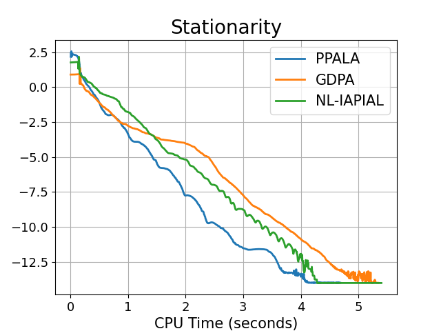
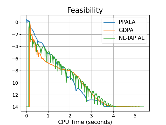
(a) QCQP with $n=200$ and $m=10$. A fixed step-size $5\times 10^{-4}$ for PPALA, and initial step-size $10^{-3}$ for GDPA and NL-IAPIAL are used.

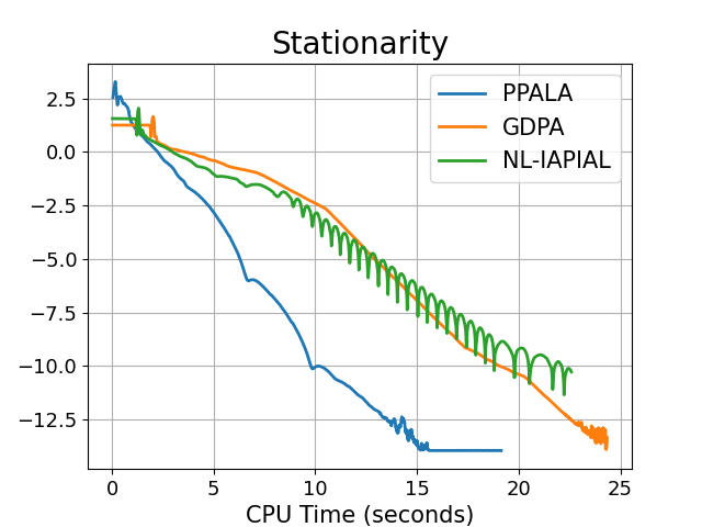
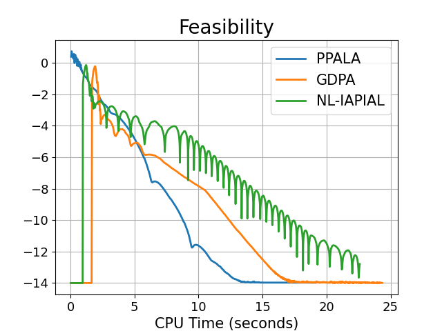
(b) QCQP with $n=1000$ and $m=10$. A fixed step-size $2\times 10^{-5}$ for PPALA and initial step-size $10^{-4}$ for GDPA and NL-IAPIAL are used.

Figure 1: Performance comparison of PPALA with GDPA and NL-IAPIAL on QCQP (V-A). All values represent the average of 5 independent runs versus CPU time in seconds. The y-axis represents $\log_{10}\left[\|\mathbf{x}_{k+1}-\Pi_{X}[\mathbf{x}_{k+1}-\nabla_{\mathbf{x}}\mathcal{L}(\mathbf{x}_{k+1},\boldsymbol{\lambda}_{k+1})]\|\right]$ and $\log_{10}\left[({1}/{\rho_{k}})\|\boldsymbol{\lambda}_{k+1}-\boldsymbol{\lambda}_{k}\|\right]$ for stationarity and feasibility, respectively.

Implementation details. The matrix $Q_{0}$ is generated as $Q_{0}=(\widetilde{Q}_{0}+\widetilde{Q}_{0}^{\top})/2$, where the entries of $\widetilde{Q}_{0}$ are randomly generated from the standard Gaussian distribution $\mathcal{N}(0,1)$. To ensure $Q_{j}$ to be positive definite, we set $Q_{j}=\widetilde{Q}_{j}+(\|\widetilde{Q}_{j}\|+1)\cdot\mathbb{I}_{n\times n}$, where $\mathbb{I}_{n\times n}$ is $n\times n$ identity matrix and the entries of $\widetilde{Q}_{j}$ are also generated from the standard Gaussian. Moreover, the vectors $c_{0}$ and $c_{j}$ are generated randomly, and $d_{j}$ is a negative value for each $j$. We set $\ell_{i}=-10$ and $u_{i}=10$ for all $i\in[n]$. To evaluate the performance of the algorithms, we use the quantity $\|\mathbf{x}_{k+1}-\Pi_{X}[\mathbf{x}_{k+1}-\nabla_{\mathbf{x}}\mathcal{L}(\mathbf{x}_{k+1},\boldsymbol{\lambda}_{k+1})]\|$ as the measure of stationarity residuals. For the measure of feasibility residuals, we use $\frac{1}{\rho_{k}}\|\boldsymbol{\lambda}_{k+1}-\boldsymbol{\lambda}_{k}\|$ for NL-IAPIAL and GDPA, and use $\frac{1}{\rho}\|\boldsymbol{\lambda}_{k+1}-\boldsymbol{\mu}_{k+1}\|$ for PPALA.

In each setting, we conduct 5 independent simulations. Given that NL-IAPIAL is a double-loop algorithm, we evaluate and compare the behaviors of the algorithms based on CPU time in seconds. We plot averaged stationary and feasibility residuals over CPU time in seconds.

Results and discussion. Figure 1 summarizes the numerical performance of PPALA, GDPA and NL-IAPIAL on QCQP problems. Figure 1(a) focuses on the problem with dimensions $n=200$ and $m=10$, while Figure 1(b) examines the larger problem with $n=1000$ and $m=10$. From the results, we observe that while there is not much difference in performance for the small-size problem ($n=200$ and $m=10$), PPALA outperforms GDPA and NL-IAPIAL for the larger problem with $n=1000$ and $m=10$. We also see that PPALA consistently reduces stationarity and feasibility residuals. This is due to the use of fixed parameters $\alpha,\beta>0$. On the other hand, we observed that GDPA exhibits a high sensitivity to the update of penalty parameters, and NL-IAPIAL needs a careful fine-tuning for inner-loop implementation. Our algorithm shows superior performance in terms of computational efficiency and robustness, maintaining its advantage as problem size increases. This emphasizes its effectiveness in handling functional constraints in large-scale non-convex optimization problems.

V-B Non-convex Multi-class Neyman-Pearson Classification

Task formulation. Next, we evaluate the performance of the proposed algorithm on a non-convex multi-class Neyman-Pearson Classification (mNPC) problem in neural network setting. The objective of this experiment is to illustrate that our algorithm can effectively handle highly non-convex constraints.

The mNPC model aims to minimize the loss for a particular class of interest while controlling the losses of others within given thresholds. Formally, consider a set of training data with $N$ classes of data, denoted by $\mathcal{D}_{i}$ for $i\in[N]$. The objective is to learn $N$ nonlinear models $f_{i}$. We predict the class of a data point $\xi$ as $\text{argmax}_{i\in[N]}f_{i}(\mathbf{x}_{i};\xi)$, where $\mathbf{x}_{i}$ represents the weights of each $f_{i}$. To obtain a high classification accuracy, the value $f_{i}(\mathbf{x}_{i};\xi)-f_{j}(\mathbf{x}_{j};\xi)$ needs to be large for any $i\neq j$ and $\xi\in\mathcal{D}_{i}$ [12], which can be obtained by minimizing the loss $\frac{1}{\lvert\mathcal{D}_{i}\rvert}\sum_{j\neq i}\sum_{\xi\in\mathcal{D}_{i}}\phi(f_{i}(\mathbf{x}_{i};\xi)-f_{j}(\mathbf{x}_{j};\xi))$. When training these $N$ nonlinear models, mNPC prioritizes minimizing the loss on one class $\mathcal{D}_{1}$, while controlling the losses on others, namely,

$$\underset{\|\mathbf{x}\|\leq\theta}{\mathrm{min}} \ \ \frac{1}{\lvert\mathcal{D}_{1}\rvert}\sum_{j\neq 1}\sum_{\xi\in\mathcal{D}_{1}}\phi(f_{1}(\mathbf{x}_{1};\xi)-f_{j}(\mathbf{x}_{j};\xi))$$

$$\mathrm{s.\>t.} \ \ \frac{1}{\lvert\mathcal{D}_{i}\rvert}\sum_{j\neq i}\sum_{\xi\in\mathcal{D}_{i}}\phi(f_{i}(\mathbf{x}_{i};\xi)-f_{j}(\mathbf{x}_{j};\xi))\leq\kappa_{i},$$

where $\ i=2,\ldots,N.$

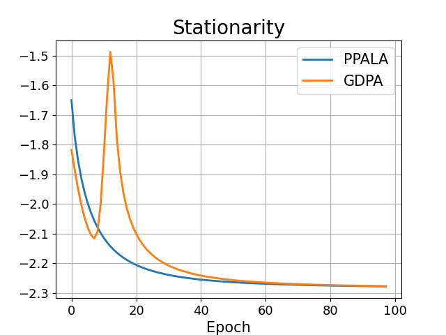
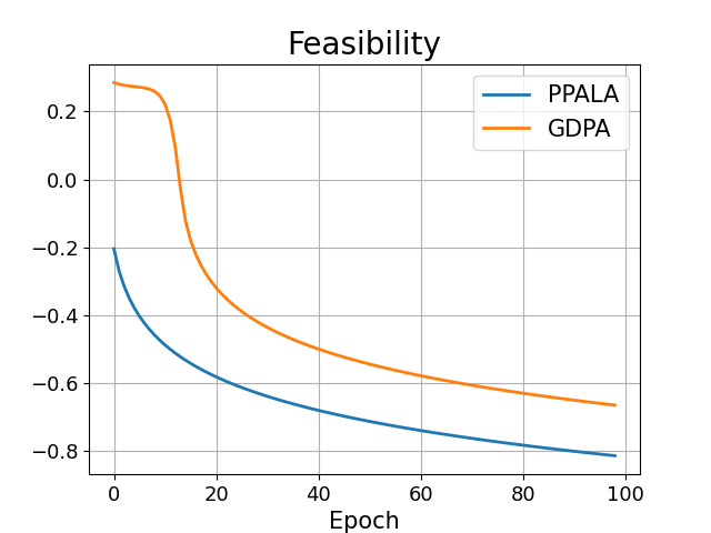
(a) Fashion-MNIST

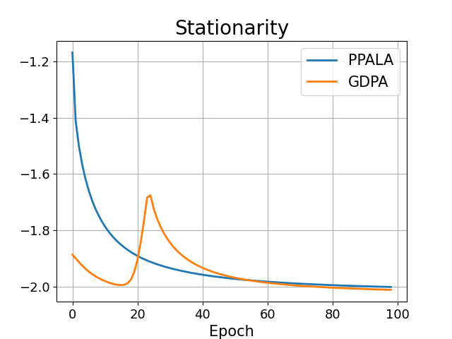
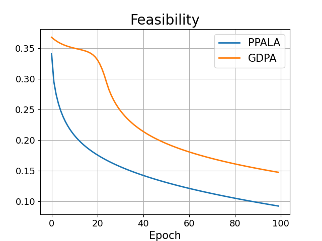
(b) CIFAR10

Figure 2: Performance comparison of PPALA and GDPA on Fashion-MNIST and CIFAR10 datasets in terms of obtaining stationarity and feasibility. We see that PPALA provides a consistent reduction of stationarity and feasibility gaps that align with our theoretical expectations. In contrast, GDPA reduces the feasibility gap at a slower rate on Fashion-MNIST and CIFAR10 in our neural network setting.

Implementation details. We use two common benchmark datasets: Fashion-MNIST [43] and CIFAR10 [20]. In the experiments, we employ a two-layer feed-forward neural network with sigmoid activation for each classifier $f_{i}$, and use batch normalization with a full batch. We compare the performance of Algorithm 1 (PPALA) with GDPA algorithm only, since NL-IAPIAL can only handle convex constraints. A sigmoid function $\phi(y)=1/{(1+\exp(y))}$ is used for the loss function as in [27]. We take 4 classes and set $\theta=1$, with $\kappa_{i}=1$ for Fashion-MNIST and $\kappa_{i}=2$ for CIFAR-10. For our algorithm, we set a fixed learning rate $10^{-3}$ for both the Fashion-MNIST and CIFAR10 cases. The initial point $\mathbf{x}_{0}$ is randomly generated in each experiment. These numerical experiments were conducted using an A100 GPU and were implemented with Pytorch [32].

Results and discussion. The performance of PPALA and GDPA are illustrated in Figure 2. We observe that PPALA converges faster than GDPA in both cases. In particular, PPALA significantly outperforms GDPA when applied to the more complex CIFAR-10 dataset, which supports the effectiveness of the PPALA. Furthermore, determining suitable parameters for PPALA was a straightforward task; $\alpha=10$ and $\beta=0.2$ were sufficient choices for both datasets. Note that the performance of PPALA is insensitive to the choice of $\alpha>0$. On the other hand, GDPA exhibits a high sensitivity to the update of its penalty parameters. For instance, we observed that GDPA fails to converge when a relatively large increase ratio is used to update the penalty parameter. Thus, it is critical to carefully select the penalty parameter to ensure GDPA’s convergence in practice. The slow infeasibility reduction in GDPA is due to the gradual update of its penalty parameter. In contrast, PPALA achieves a fast and consistent reduction in infeasibility with the fixed parameter $\rho=\frac{\alpha}{1+\alpha\beta}$.

These results emphasize the effectiveness and robustness of our PPALA compared to GDPA, especially in the context of more complex datasets such as CIFAR10 and highly non-convex constraints such as neural networks.

VI Conclusions

In this work, we proposed a novel single-loop primal-dual algorithm to solve non-convex functional constrained optimization problems. We show that our method can achieves an improved complexity bound of $\widetilde{\mathcal{O}}(1/\epsilon^{2})$ with performance guarantees. The proposed method ensures a consistent reduction in stationarity and feasibility gaps under mild conditions. The experimental results demonstrate that our algorithm performs better than the existing single-loop algorithm. Future research could consider extending this simple optimization method to solve stochastic non-convex constrained optimization problems, which will result in a broader application domain in sigmal processing and machine learning.

Appendix A Proof of Lemma 10

Proof.

Writing the optimality condition for the $\mathbf{x}$-update (10), we have that for all $k\geq 0$

$$\nabla_{\mathbf{x}}\ell_{\rho}(\mathbf{w}_{k})+\frac{1}{\eta}(\mathbf{x}_{k+1}-\mathbf{x}_{k})+\mathbf{d}_{k+1}=\mathbf{0},\ \ \mathbf{d}_{k+1}\in\partial r(\mathbf{x}_{k+1}).$$ (38)

Using the subdifferential calculus rules, we also get

$$\nabla_{\mathbf{x}}\ell_{\rho}(\mathbf{w}_{k+1})+\mathbf{d}_{k+1}\in\partial_{\mathbf{x}}\mathcal{L}_{\rho}(\mathbf{w}_{k+1}).$$ (39)

Hence, by defining the quantity

$$\zeta_{\mathbf{x}}^{k+1}:=\nabla_{\mathbf{x}}\ell_{\rho}(\mathbf{w}_{k+1})-\nabla_{\mathbf{x}}\ell_{\rho}(\mathbf{w}_{k})+\frac{1}{\eta}(\mathbf{x}_{k}-\mathbf{x}_{k+1}),$$

and using (38) and (39), we obtain $\zeta_{\mathbf{x}}^{k+1}\in\partial_{\mathbf{x}}\mathcal{L}_{\rho}(\mathbf{w}_{k+1}).$

Next, define the quantity

$$\zeta_{\mathbf{u}}^{k+1}:=\mathbf{u}_{k+1}-\Pi_{[0,U]}[\mathbf{u}_{k+1}-(\boldsymbol{\lambda}_{k+1}+\rho(g(\mathbf{x}_{k+1})+\mathbf{u}_{k+1})],$$

which is equivalent to the projected gradient of $\mathcal{L}_{\rho}$ in $\mathbf{u}$ as a measure of optimality for $\mathbf{u}$-update:

$$\widetilde{\nabla}_{\mathbf{u}}\mathcal{L}_{\rho}(\mathbf{w}_{k+1})$$

$$=\mathbf{u}_{k+1}-\underset{\mathbf{v}\in{[0,U]}}{\mathrm{argmin}}\left\{\left\langle\nabla_{\mathbf{u}}\mathcal{L}_{\rho}(\mathbf{w}_{k+1}),\mathbf{v}-\mathbf{u}_{k+1}\right\rangle\right.$$

$$\hskip 79.49744pt\left.+({1}/{2})\|\mathbf{v}-\mathbf{u}_{k+1}\|^{2}\right\}$$

$$=\mathbf{u}_{k+1}-\Pi_{[0,U]}[\mathbf{u}_{k+1}-(\boldsymbol{\lambda}_{k+1}+(g(\mathbf{x}_{k+1})+\mathbf{u}_{k+1})].$$

Hence, we obtain

$$\zeta_{\mathbf{x}}^{k+1}\in\partial_{\mathbf{x}}\mathcal{L}_{\rho}(\mathbf{w}_{k+1}),\ \ \text{and}\ \ \zeta_{\mathbf{u}}^{k+1}=\widetilde{\nabla}_{\mathbf{u}}\mathcal{L}_{\rho}(\mathbf{w}_{k+1}).$$

From the $\mathbf{z}$-update (14), it immediately follows that

$$\nabla_{\mathbf{z}}\mathcal{L}_{\rho}(\mathbf{w}_{k+1})=\alpha\mathbf{z}_{k+1}-(\boldsymbol{\lambda}_{k+1}-\boldsymbol{\mu}_{k+1})=\mathbf{0},$$

Hence, we obtain

$$\boldsymbol{\zeta}_{\mathbf{p}}^{k+1}:=\begin{pmatrix}\zeta_{\mathbf{x}}^{k+1}&\in\partial_{\mathbf{x}}\mathcal{L}_{\rho}(\mathbf{x}_{k+1},\mathbf{u}_{k+1},\mathbf{z}_{k+1},\boldsymbol{\lambda}_{k+1},\boldsymbol{\mu}_{k+1})\\ \zeta_{\mathbf{u}}^{k+1}&=\widetilde{\nabla}_{\mathbf{u}}\mathcal{L}_{\rho}(\mathbf{x}_{k+1},\mathbf{u}_{k+1},\mathbf{z}_{k+1},\boldsymbol{\lambda}_{k+1},\boldsymbol{\mu}_{k+1})\\ \mathbf{0}&=\nabla_{\mathbf{z}}\mathcal{L}_{\rho}(\mathbf{x}_{k+1},\mathbf{u}_{k+1},\mathbf{z}_{k+1},\boldsymbol{\lambda}_{k+1},\boldsymbol{\mu}_{k+1})\\ \end{pmatrix}.$$

We derive upper estimates for $\zeta_{\mathbf{x}}^{k+1}$ and $\zeta_{\mathbf{u}}^{k+1}$. A straightforward calculation yields

$$\|\zeta_{\mathbf{x}}^{k+1}\|\leq \|\nabla f(\mathbf{x}_{k+1})-\nabla f(\mathbf{x}_{k})\|+(1/{\eta})\|\mathbf{x}_{k}-\mathbf{x}_{k+1}\|$$

$$+\|\nabla g(\mathbf{x}_{k+1})(\boldsymbol{\lambda}_{k+1}+\rho(g(\mathbf{x}_{k+1})+\mathbf{u}_{k+1})$$

$$\qquad\qquad\quad-\nabla g(\mathbf{x}_{k})(\boldsymbol{\lambda}_{k}+\rho(g(\mathbf{x}_{k})+\mathbf{u}_{k})\|$$

$$\leq (L_{f}+1/\eta)\|\mathbf{x}_{k+1}-\mathbf{x}_{k}\|$$

$$+\|\nabla g(\mathbf{x}_{k+1})\boldsymbol{\lambda}_{k+1}-\nabla g(\mathbf{x}_{k})\boldsymbol{\lambda}_{k+1}$$

$$\qquad\qquad\quad+\nabla g(\mathbf{x}_{k})\boldsymbol{\lambda}_{k+1}-\nabla g(\mathbf{x}_{k})\boldsymbol{\lambda}_{k}\|$$ (40a)

$$+\rho\|\nabla g(\mathbf{x}_{k+1})g(\mathbf{x}_{k+1})-\nabla g(\mathbf{x}_{k})g(\mathbf{x}_{k+1})$$

$$\quad\quad\ \ +\nabla g(\mathbf{x}_{k})g(\mathbf{x}_{k+1})-\nabla g(\mathbf{x}_{k})g(\mathbf{x}_{k})\|$$ (40b)

$$+\rho\|\nabla g(\mathbf{x}_{k+1})\mathbf{u}_{k+1}-\nabla g(\mathbf{x}_{k})\mathbf{u}_{k+1}$$

$$\qquad\qquad\quad+\nabla g(\mathbf{x}_{k})\mathbf{u}_{k+1}-\nabla g(\mathbf{x}_{k})\mathbf{u}_{k}\|,$$ (40c)

in which (40a), (40b), and (40c) can be bounded by

$$\eqref{eq:xi_x1} \leq B_{\boldsymbol{\lambda}}L_{g}\|\mathbf{x}_{k+1}-\mathbf{x}_{k}\|+M_{g}\|\boldsymbol{\lambda}_{k+1}-\boldsymbol{\lambda}_{k}\|$$

$$\leq B_{\boldsymbol{\lambda}}L_{g}\|\mathbf{x}_{k+1}-\mathbf{x}_{k}\|+\rho M_{g}^{2}\|\mathbf{x}_{k+1}-\mathbf{x}_{k}\|$$

$$\quad+\rho M_{g}\|\mathbf{u}_{k+1}-\mathbf{u}_{k}\|+M_{g}\|\boldsymbol{\mu}_{k+1}-\boldsymbol{\mu}_{k}\|$$

$$\leq\left(B_{\boldsymbol{\lambda}}L_{g}+\rho M_{g}^{2}\right)\|\mathbf{x}_{k+1}-\mathbf{x}_{k}\|$$

$$\quad+\rho M_{g}\|\mathbf{u}_{k+1}-\mathbf{u}_{k}\|+M_{g}{\delta_{k}};$$

$$\eqref{eq:xi_x2} \leq(\rho B_{g}L_{g}+\rho M_{g}^{2})\|\mathbf{x}_{k+1}-\mathbf{x}_{k}\|;$$

$$\eqref{eq:xi_x3} \leq\rho B_{\mathbf{u}}L_{g}\|\mathbf{x}_{k+1}-\mathbf{x}_{k}\|+\rho M_{g}\|\mathbf{u}_{k+1}-\mathbf{u}_{k}\|.$$

where for bounding (40a), we used the $\boldsymbol{\lambda}$-update and $\|\boldsymbol{\mu}_{k+1}-\boldsymbol{\mu}_{k}\|=\frac{\delta_{k}}{\|\boldsymbol{\lambda}_{k}-\boldsymbol{\mu}_{k}\|+\frac{1}{\|\boldsymbol{\lambda}_{k}-\boldsymbol{\mu}_{k}\|}}\leq{\delta_{k}}.$ Hence,

$$\|\zeta_{\mathbf{x}}^{k+1}\|$$

$$\leq(L_{f}+{1}/{\eta}+B_{\boldsymbol{\lambda}}L_{g}+\rho L_{g}(B_{g}+B_{\mathbf{u}}+2M_{g}^{2}))\|\mathbf{x}_{k+1}-\mathbf{x}_{k}\|$$

$$\quad+2\rho M_{g}\|\mathbf{u}_{k+1}-\mathbf{u}_{k}\|+M_{g}{\delta_{k}}.$$ (42)

Next, we estimate an upper bound for the component $\zeta_{\mathbf{u},k+1}$. To simplify notation, define

$$\widetilde{\mathbf{u}}_{k+1} =\underset{\mathbf{v}\in{[0,U]}}{\mathrm{argmin}}\left\{\left\langle\nabla_{\mathbf{u}}\mathcal{L}_{\rho}(\mathbf{w}_{k+1}),\mathbf{v}-\mathbf{u}_{k+1}\right\rangle\right.$$

$$\hskip 50.58878pt\left.+({1}/{2})\|\mathbf{v}-\mathbf{u}_{k+1}\|^{2}\right\}.$$

Clearly, $\|\zeta_{\mathbf{u},k+1}\|=\|\mathbf{u}_{k+1}-\widetilde{\mathbf{u}}_{k+1}\|.$ The first-order optimality condition implies that

$$\left\langle\nabla_{\mathbf{u}}\mathcal{L}_{\rho}(\mathbf{u}_{k+1})+(\widetilde{\mathbf{u}}_{k+1}-\mathbf{u}_{k+1}),\mathbf{u}-\widetilde{\mathbf{u}}_{k+1}\right\rangle\geq 0.$$ (43)

Here, $\nabla_{\mathbf{u}}\mathcal{L}_{\rho}(\mathbf{w}_{k+1})$ is denoted by $\nabla_{\mathbf{u}}\mathcal{L}_{\rho}(\mathbf{u}_{k+1})$. Note that the $\mathbf{u}$-update (11) is equivalent to

$$\mathbf{u}_{k+1}=\underset{\mathbf{u}\in[0,U]}{\mathrm{argmin}}\left\{\left\langle\nabla_{\mathbf{u}}\mathcal{L}_{\rho}(\mathbf{u}_{k}),\mathbf{u}-\mathbf{u}_{k}\right\rangle+\frac{1}{2\tau}\|\mathbf{u}-\mathbf{u}_{k}\|^{2}\right\},$$

where $\nabla_{\mathbf{u}}\mathcal{L}_{\rho}(\mathbf{u}_{k})=\nabla_{\mathbf{u}}\mathcal{L}_{\rho}(\mathbf{x}_{k+1},\mathbf{u}_{k},\mathbf{z}_{k},\boldsymbol{\lambda}_{k},\boldsymbol{\mu}_{k})$. By the first-order optimality condition, we have

$$\left\langle\nabla_{\mathbf{u}}\mathcal{L}_{\rho}(\mathbf{u}_{k})+\frac{1}{\tau}(\mathbf{u}_{k+1}-\mathbf{u}_{k}),{\mathbf{u}}-\mathbf{u}_{k+1}\right\rangle\geq 0.$$ (44)

Combining (43) and (44), with settings $\mathbf{u}=\mathbf{u}_{k+1}$ in (43) and $\mathbf{u}=\widetilde{\mathbf{u}}_{k+1}$ in (44), yields

$$\left\langle\nabla_{\mathbf{u}}\mathcal{L}_{\rho}(\mathbf{u}_{k})-\nabla_{\mathbf{u}}\mathcal{L}_{\rho}(\mathbf{u}_{k+1})+{\tau}^{-1}(\mathbf{u}_{k+1}-\mathbf{u}_{k})\right.\\ \left.-(\widetilde{\mathbf{u}}_{k+1}-\mathbf{u}_{k+1}),\widetilde{\mathbf{u}}_{k+1}-\mathbf{u}_{k+1}\right\rangle\geq 0,$$ (45)

equivalently,

$$\left\langle\nabla_{\mathbf{u}}\mathcal{L}_{\rho}(\mathbf{u}_{k})-\nabla_{\mathbf{u}}\mathcal{L}_{\rho}(\mathbf{u}_{k+1})+{\tau}^{-1}(\mathbf{u}_{k+1}-\mathbf{u}_{k}),\right.\\ \left.\widetilde{\mathbf{u}}_{k+1}-\mathbf{u}_{k+1}\right\rangle\geq\|\widetilde{\mathbf{u}}_{k+1}-\mathbf{u}_{k+1}\|^{2}.$$ (46)

Applying the Cauchy-Schwarz inequality yields

$$\left(\|\nabla_{\mathbf{u}}\mathcal{L}_{\rho}(\mathbf{u}_{k})-\nabla_{\mathbf{u}}\mathcal{L}_{\rho}(\mathbf{u}_{k+1})\|+{\tau}^{-1}\|\mathbf{u}_{k+1}-\mathbf{u}_{k}\|\right)\cdot\\ \|\widetilde{\mathbf{u}}_{k+1}-\mathbf{u}_{k+1}\|\geq\|\widetilde{\mathbf{u}}_{k+1}-\mathbf{u}_{k+1}\|^{2},$$ (47)

where

$$\quad\ \|\nabla_{\mathbf{u}}\mathcal{L}_{\rho}(\mathbf{u}_{k})-\nabla_{\mathbf{u}}\mathcal{L}_{\rho}(\mathbf{u}_{k+1})\|$$

$$=\|\nabla_{\mathbf{u}}\mathcal{L}_{\rho}(\mathbf{x}_{k+1},\mathbf{u}_{k},\mathbf{z}_{k},\boldsymbol{\lambda}_{k},\boldsymbol{\mu}_{k})$$

$$\hskip 36.135pt-\nabla_{\mathbf{u}}\mathcal{L}_{\rho}(\mathbf{x}_{k+1},\mathbf{u}_{k+1},\mathbf{z}_{k+1},\boldsymbol{\lambda}_{k+1},\boldsymbol{\mu}_{k+1})\|$$

$$\leq\|\boldsymbol{\lambda}_{k}+\rho(g(\mathbf{x}_{k+1})+\mathbf{u}_{k})-\boldsymbol{\lambda}_{k+1}-\rho(g(\mathbf{x}_{k+1})+\mathbf{u}_{k+1})\|$$

$$\leq\rho(M_{g}\|\mathbf{x}_{k+1}-\mathbf{x}_{k}\|+2\|\mathbf{u}_{k+1}-\mathbf{u}_{k}\|+\delta_{k}).$$

Therefore,

$$\|\zeta_{\mathbf{u}}^{k+1}\|=\|\widetilde{\mathbf{u}}_{k+1}-\mathbf{u}_{k+1}\|$$

$$\leq\rho M_{g}\|\mathbf{x}_{k+1}-\mathbf{x}_{k}\|+\left(2\rho+{\tau}^{-1}\right)\|\mathbf{u}_{k+1}-\mathbf{u}_{k}\|+\delta_{k}.$$ (48)

Combining (42) and (48), we obtain

$$\|\boldsymbol{\zeta}_{\mathbf{p}}^{k+1}\|\leq d_{1}(\|\mathbf{x}_{k+1}-\mathbf{x}_{k}\|+\|\mathbf{u}_{k+1}-\mathbf{u}_{k}\|)+(M_{g}+1)\delta_{k},$$

where $d_{1}=\max\{L_{f}+B_{\boldsymbol{\lambda}}L_{g}+\rho(M_{g}+B_{g}L_{g}+B_{\mathbf{u}}L_{g}+2M_{g}^{2})\\ +{1}/{\eta},2\rho(M_{g}+1)+{1}/{\tau}\}.$ This inequality, combined with $\boldsymbol{\zeta}_{\mathbf{p}}^{k+1}\in\partial_{\mathbf{p}}\mathcal{L}_{\rho}(\mathbf{w}_{k+1})$, yields the desired result. ∎

References

- [1] R. Andreani, G. Haeser, M. L. Schuverdt, L. D. Secchin, and P. J. Silva. On scaled stopping criteria for a safeguarded augmented lagrangian method with theoretical guarantees. Mathematical Programming Computation, 14(1):121–146, 2022.
- [2] D. P. Bertsekas. Nonlinear programming. Athena scientific Belmont, 1999.
- [3] D. P. Bertsekas. Constrained optimization and Lagrange multiplier methods. Academic press, 2014.
- [4] E. G. Birgin and J. M. Martínez. Practical augmented Lagrangian methods for constrained optimization. SIAM, 2014.
- [5] J. Bolte, S. Sabach, and M. Teboulle. Proximal alternating linearized minimization or nonconvex and nonsmooth problems. Mathematical Programming, 146(1-2):459–494, 2014.
- [6] J. Bolte, S. Sabach, and M. Teboulle. Nonconvex Lagrangian-based optimization: monitoring schemes and global convergence. Mathematics of Operations Research, 2018.
- [7] D. Boob, Q. Deng, and G. Lan. Stochastic first-order methods for convex and nonconvex functional constrained optimization. Mathematical Programming, pages 1–65, 2022.
- [8] R. I. Boţ, E. R. Csetnek, and D.-K. Nguyen. A proximal minimization algorithm for structured nonconvex and nonsmooth problems. SIAM Journal on Optimization, 29(2):1300–1328, 2019.
- [9] R. I. Boţ and D.-K. Nguyen. The proximal alternating direction method of multipliers in the nonconvex setting: convergence analysis and rates. Mathematics of Operations Research, 2020.
- [10] S. Boyd, N. Parikh, and E. Chu. Distributed optimization and statistical learning via the alternating direction method of multipliers. Now Publishers Inc, 2011.
- [11] C. Cartis, N. I. Gould, and P. L. Toint. On the evaluation complexity of composite function minimization with applications to nonconvex nonlinear programming. SIAM Journal on Optimization, 21(4):1721–1739, 2011.
- [12] K. Crammer and Y. Singer. On the learnability and design of output codes for multiclass problems. Machine learning, 47:201–233, 2002.
- [13] G. N. Grapiglia and Y.-x. Yuan. On the complexity of an augmented lagrangian method for nonconvex optimization. IMA Journal of Numerical Analysis, 41(2):1546–1568, 2021.
- [14] G. Haeser, O. Hinder, and Y. Ye. On the behavior of lagrange multipliers in convex and nonconvex infeasible interior point methods. Mathematical Programming, pages 1–32, 2019.
- [15] D. Hajinezhad and M. Hong. Perturbed proximal primal–dual algorithm for nonconvex nonsmooth optimization. Mathematical Programming, 176(1-2):207–245, 2019.
- [16] M. R. Hestenes. Multiplier and gradient methods. Journal of optimization theory and applications, 4(5):303–320, 1969.
- [17] L. Huang and N. Vishnoi. Stable and fair classification. In International Conference on Machine Learning, pages 2879–2890. PMLR, 2019.
- [18] W. Kong, J. G. Melo, and R. D. Monteiro. Iteration complexity of a proximal augmented lagrangian method for solving nonconvex composite optimization problems with nonlinear convex constraints. Mathematics of Operations Research, 2022.
- [19] W. Kong, J. G. Melo, and R. D. Monteiro. Iteration complexity of an inner accelerated inexact proximal augmented lagrangian method based on the classical lagrangian function. SIAM Journal on Optimization, 33(1):181–210, 2023.
- [20] A. Krizhevsky, G. Hinton, et al. Learning multiple layers of features from tiny images. 2009.
- [21] G. Lan and R. D. Monteiro. Iteration-complexity of first-order augmented lagrangian methods for convex programming. Mathematical Programming, 155(1-2):511–547, 2016.
- [22] G. Li and T. K. Pong. Global convergence of splitting methods for nonconvex composite optimization. SIAM Journal on Optimization, 25(4):2434–2460, 2015.
- [23] Z. Li, P.-Y. Chen, S. Liu, S. Lu, and Y. Xu. Rate-improved inexact augmented Lagrangian method for constrained nonconvex optimization. In International Conference on Artificial Intelligence and Statistics, pages 2170–2178. PMLR, 2021.
- [24] Z. Li and Y. Xu. Augmented lagrangian–based first-order methods for convex-constrained programs with weakly convex objective. INFORMS Journal on Optimization, 3(4):373–397, 2021.
- [25] Q. Lin, R. Ma, and Y. Xu. Complexity of an inexact proximal-point penalty method for constrained smooth non-convex optimization. Computational Optimization and Applications, 82(1):175–224, 2022.
- [26] Y.-F. Liu, X. Liu, and S. Ma. On the nonergodic convergence rate of an inexact augmented lagrangian framework for composite convex programming. Mathematics of Operations Research, 44(2):632–650, 2019.
- [27] S. Lu. A single-loop gradient descent and perturbed ascent algorithm for nonconvex functional constrained optimization. In International Conference on Machine Learning, pages 14315–14357. PMLR, 2022.
- [28] Z. Lu and Z. Zhou. Iteration-complexity of first-order augmented lagrangian methods for convex conic programming. SIAM Journal on Optimization, 33(2):1159–1190, 2023.
- [29] Z.-Q. Luo, W.-K. Ma, A. M.-C. So, Y. Ye, and S. Zhang. Semidefinite relaxation of quadratic optimization problems. IEEE Signal Processing Magazine, 27(3):20–34, 2010.
- [30] A. S. Nemirovskij and D. B. Yudin. Problem complexity and method efficiency in optimization. Wiley-Interscience, 1983.
- [31] Y. Ouyang, Y. Chen, G. Lan, and E. Pasiliao Jr. An accelerated linearized alternating direction method of multipliers. SIAM Journal on Imaging Sciences, 8(1):644–681, 2015.
- [32] A. Paszke, S. Gross, F. Massa, A. Lerer, J. Bradbury, G. Chanan, T. Killeen, Z. Lin, N. Gimelshein, L. Antiga, et al. Pytorch: An imperative style, high-performance deep learning library. Advances in neural information processing systems, 32, 2019.
- [33] M. J. Powell. A method for nonlinear constraints in minimization problems. Optimization, pages 283–298, 1969.
- [34] P. Rigollet and X. Tong. Neyman-pearson classification, convexity and stochastic constraints. Journal of Machine Learning Research, 2011.
- [35] R. T. Rockafellar and R. J.-B. Wets. Variational analysis, volume 317. Springer Science & Business Media, 2009.
- [36] M. F. Sahin, A. Alacaoglu, F. Latorre, V. Cevher, et al. An inexact augmented Lagrangian framework for nonconvex optimization with nonlinear constraints. In Advances in Neural Information Processing Systems, pages 13943–13955, 2019.
- [37] G. Scutari, F. Facchinei, and L. Lampariello. Parallel and distributed methods for constrained nonconvex optimization—part i: Theory. IEEE Transactions on Signal Processing, 65(8):1929–1944, 2016.
- [38] G. Scutari, F. Facchinei, L. Lampariello, S. Sardellitti, and P. Song. Parallel and distributed methods for constrained nonconvex optimization-Part II: Applications in communications and machine learning. IEEE Transactions on Signal Processing, 65(8):1945–1960, 2016.
- [39] G. Scutari, F. Facchinei, P. Song, D. P. Palomar, and J.-S. Pang. Decomposition by partial linearization: Parallel optimization of multi-agent systems. IEEE Transactions on Signal Processing, 62(3):641–656, 2014.
- [40] Q. Shi, M. Hong, X. Fu, and T.-H. Chang. Penalty dual decomposition method for nonsmooth nonconvex optimization—Part II: Applications. IEEE Transactions on Signal Processing, 68:4242–4257, 2020.
- [41] M. V. Solodov. Global convergence of an sqp method without boundedness assumptions on any of the iterative sequences. Mathematical programming, 118(1):1–12, 2009.
- [42] K. Sun and A. Sun. Dual descent alm and admm. arXiv preprint arXiv:2109.13214, 2021.
- [43] H. Xiao, K. Rasul, and R. Vollgraf. Fashion-mnist: a novel image dataset for benchmarking machine learning algorithms. arXiv preprint arXiv:1708.07747, 2017.
- [44] Y. Xie and S. J. Wright. Complexity of proximal augmented Lagrangian for nonconvex optimization with nonlinear equality constraints. Journal of Scientific Computing, 86(3):1–30, 2021.
- [45] Y. Xu. Accelerated first-order primal-dual proximal methods for linearly constrained composite convex programming. SIAM Journal on Optimization, 27(3):1459–1484, 2017.
- [46] Y. Xu. Iteration complexity of inexact augmented lagrangian methods for constrained convex programming. Mathematical Programming, 185:199–244, 2021.
- [47] M. B. Zafar, I. Valera, M. Gomez-Rodriguez, and K. P. Gummadi. Fairness constraints: A flexible approach for fair classification. The Journal of Machine Learning Research, 20(1):2737–2778, 2019.
- [48] J. Zhang and Z.-Q. Luo. A proximal alternating direction method of multiplier for linearly constrained nonconvex minimization. SIAM Journal on Optimization, 30(3):2272–2302, 2020.
- [49] J. Zhang and Z.-Q. Luo. A global dual error bound and its application to the analysis of linearly constrained nonconvex optimization. SIAM Journal on Optimization, 32(3):2319–2346, 2022.