Perturbed Decision-Focused Learning
for Modeling Strategic Energy Storage

Ming Yi, Member, IEEE, Saud Alghumayjan, Student Member, IEEE, Bolun Xu, Member, IEEE, This work was supported in part by the Data Science Institute in Columbia University and in part by the National Science Foundation under award ECCS-2239046. (Corresponding author: Ming Yi.) Ming Yi is with the Data Science Institute, Columbia University, New York City, NY. Saud Alghumayjan, and Bolun Xu are with Earth and Environmental Engineering, Columbia University, New York City, NY. Email:{my2826, saa2244, bx2177}@columbia.edu.
Abstract

This paper presents a novel decision-focused framework integrating the physical energy storage model into machine learning pipelines. Motivated by the model predictive control for energy storage, our end-to-end method incorporates the prior knowledge of the storage model and infers the hidden reward that incentivizes energy storage decisions. This is achieved through a dual-layer framework, combining a prediction layer with an optimization layer. We introduce the perturbation idea into the designed decision-focused loss function to ensure the differentiability over linear storage models, supported by a theoretical analysis of the perturbed loss function. We also develop a hybrid loss function for effective model training. We provide two challenging applications for our proposed framework: energy storage arbitrage, and energy storage behavior prediction. The numerical experiments on real price data demonstrate that our arbitrage approach achieves the highest profit against existing methods. The numerical experiments on synthetic and real-world energy storage data show that our approach achieves the best behavior prediction performance against existing benchmark methods, which shows the effectiveness of our method.

Index Terms:
Differentiable Decision-Focused Framework, Energy Storage Arbitrage, Perturbation Idea, Energy Storage Behavior

I Introduction

Over the past decade, energy storage integration has proven essential for economic and reliable power system decarbonization [1]. However, integrating storage presents unique challenges: energy storage must strategically plan its operations based on future price expectations to quantify its opportunity value, given its limited energy capacity [2, 3]. For instance, in price arbitrage—the most popular grid service for energy storage in North America—storage must accurately predict future prices, especially price spikes, and valleys, to determine the optimal times to charge and discharge. In practice, most energy storage owners adopt a model predictive control (MPC) framework, which decouples price prediction from storage control. They develop proprietary electricity price predictors to capture market fluctuations and input the predicted prices into arbitrage optimization models.

However, decoupling prediction and optimization in MPC frameworks introduces storage control and regulation challenges. For storage operators, machine learning predictors often struggle to effectively account for how their predictions will be utilized in the physical energy storage model, particularly given the limited data availability and computing power in practical implementations [4]. Conversely, electricity market regulators are concerned that non-transparent storage arbitrage models may enable storage operators to exercise market power [5], thereby impeding the convergence of social welfare. Regulators seek systematic approaches to navigate storage operators’ proprietary prediction models and understand the correlation between strategic storage behaviors and market price dynamics.

This paper proposes a decision-focused framework incorporating an energy storage model as a perturbed differentiable layer in the learning pipeline. Our proposed framework offers a significant advantage over existing decision-focused approaches [6] in that it does not rely on ground truth prediction information. The result learning model is more efficient at both predicting and optimizing storage operation from the perspective of storage operators or regulators. The contributions of this paper include:

  • We develop a decision-focused, end-to-end pipeline incorporating the physical energy storage model. The proposed framework includes a prediction layer to infer the hidden reward and an optimization layer to model the decision-making of energy storage.

  • We exploit the perturbation idea to solve the differentiable issue in the decision-focused loss function. We also add a predictor regularizer in the loss function to enhance the prediction performance.

  • We provide a theoretical analysis for the perturbed loss function. Specifically, we prove that the perturbed loss function is convex and that its gradient is Lipschitz continuous. We also show the connection between the perturbed loss function and the original loss function.

  • We validate the proposed framework through two applications: energy storage arbitrage and forecasting the energy storage behavior. To the best of our knowledge, this specific formulation for both applications has not been studied before.

  • The numerical experiments for two applications on synthetic datasets and real-world datasets demonstrate that our approach outperforms the benchmark methods.

The rest of the paper is organized as follows. Section II reviews the related works. Section III introduces the formulation. Section IV presents our proposed end-to-end approach. The numerical results are reported in Section V, and Section VI concludes our paper.

II Motivation and Related Works

II-A Learning-aided Storage Operation

Storage owners can arbitrage electricity prices by charging energy when prices are low and selling it back when prices are high. They can submit bids in the day-ahead market (DAM) and the real-time market (RTM), each with its own market clearing timelines and rules. Various methods have been proposed, such as bi-level optimization [7] and dynamic programming [8] [9]. For small-scale energy storage, such as Behind-the-Meter (BTM) energy storage, owners can self-schedule operations without informing the system operator. Many approaches have been proposed, including dynamical programming [10], model predictive control (MPC) [11][12], and reinforcement learning [13]. Electricity price fluctuations are the most critical factor in deciding the best bid or schedule options. Various models have been developed over the years to address this uncertainty, employing techniques such as Markov process models [14], frequency analysis [15], and deep neural networks [16, 17].

II-B Learning-aided Storage Monitoring

There is increasing interest in understanding and modeling how energy-limited resources, including storage and demand-side resources, would behave in electricity markets. One line of related works is modeling the demand response behavior. Both model-based and data-driven approaches are proposed to model the price-responsive behaviors. The model-based approaches [18] [19] first solve a bi-level optimization problem to identify the model parameter and then forecast the future demand response behaviors of buildings. For data-driven approaches, reference [20] employs the Gaussian process to model the demand response of a building with energy storage. [21] builds a neural network to model customer’s demand response behaviors.

The most relevant research is the energy storage model identification [22] [23], which aims to identify the unknown parameters of the energy storage model and uses a pre-built price predictor to forecast the energy storage behavior based on the identified model. On the one hand, knowing the actual price predictor the energy storage owner uses is difficult. Instead, the system operator usually can only observe the historical energy storage behaviors. On the other hand, the price predictor mainly focuses on predicting the mean value of the price trend but falls short of capturing the price variations. The behaviors of energy storage arbitrage are based on the price spread instead of the true price value. Therefore, simply feeding the price prediction into the optimization model may not predict the energy storage behavior well.

II-C Decision-Focused Learning

Decision-focused learning has gained increasing interest in overcoming the limitations of the MPC-type methods in which the prediction model often fails to leverage the structural information by the optimization constraints and objective functions. One approach is a smart predict-then-optimize framework that integrates optimization into the prediction model and develops a decision-focused surrogate loss function[24, 25]. This line of research requires the ground truth prediction information for the model training. Another promising line of research is the learning-by-experience approach [26, 27]. Without costly labeled ground truth prediction data, this method only requires optimal decision information and shows its efficacy in addressing vehicle routing problems.

Energy storage models have mixed cost terms, including linear and quadratic costs, along with charging/discharging dynamics governed by state-of-charge evolution. The aforementioned methods mainly focus on linear cost functions and lack consideration for the unique characteristics of energy storage systems. While existing work [6] extends the smart predict-then-optimize paradigm to energy storage arbitrage problems, they do not consider degradation costs and depend on perfect forecasting pricing data for model training. Our approach distinguishes [6] by only requiring energy storage decisions rather than relying on ground truth prediction data for training model. This is particular helpful for the scenarios where the ground truth prediction data is not available. Therefore, we broaden the applicability of decision-focused learning, making it adaptable to various scenarios and offering a more comprehensive solution for strategic energy storage applications.

III Problem Formulation

We first introduce the storage model and the baseline MPC framework, then formulate the learning problem.

III-A Energy Storage Arbitrage Model

We consider a model-predictive control (MPC) type storage arbitrage controller in which the storage operator uses a pre-trained model $g(\bm{x})$ to generate price predictions using historical features $\bm{x}$, and then the storage model makes the optimal arbitrage decisions by solving (1).

$\displaystyle(\bar{p}_{t},\bar{b}_{t})\in\underset{{p_{t},b_{t}}\in\mathcal{X}}{\textbf{argmax}}\;$ $\displaystyle\sum_{t=1}^{T}{\lambda}_{t}(p_{t}-b_{t})-u(p_{t},b_{t})\,,\;\bm{{\lambda}}=g(\bm{x})$ (1a)
s.t. $\displaystyle 0\leq p_{t},b_{t}\leq P$ (1b)
$\displaystyle p_{t}=0\quad\text{if}\quad\lambda_{t}<0$ (1c)
$\displaystyle 0\leq e_{t}\leq E$ (1d)
$\displaystyle e_{t}-e_{t-1}=-p_{t}/\eta+b_{t}\eta$ (1e)

where $p_{t}$ and $b_{t}$ are discharge and charge power at time $t$, while $\bar{p}_{t}$ and $\bar{b}_{t}$ are the optimized storage dispatch decisions. $T$ is the time horizon. $\lambda_{t}$ is the predicted real-time price. $e_{t}$ is the state-of-charge (SoC). $P$ is the power rating of storage. $\eta$ is the storage efficiency. $E$ is the SoC capacity. $u(p_{t},b_{t})$ is the charge/discharge cost term and it is a convex function over $p_{t},b_{t}$. For example, $u(p_{t},b_{t})=C_{1}p_{t}+C_{2}p_{t}^{2}+C_{3}b_{t}+C_{4}b_{t}^{2}$ models the linear and quadratic discharging cost. The objective of the arbitrage model is to maximize its profit while keeping the charge/discharge decision within the physical constraints. (1b) sets the upper and lower bounds for the charge and discharge power. (1c) is a sufficient condition to enforce the storage not to charge and discharge at the same time [9]. (1d) sets the upper and lower bounds for SoC. (1e) models the SoC evolution process. In the following, we denote the constraints in (1b)-(1e) as the feasibility set $\mathcal{X}$.

III-B Problem Statement

Our algorithm aims to infer the hidden reward $\hat{\bm{{\lambda}}}$ that steers the storage operation to achieve the observed energy storage strategy (charge/discharge decisions). Subsequently, we use this predicted reward to imitate the observed strategy in future energy storage decisions. In particular, our goal is to establish an end-to-end mapping for predicting forthcoming energy storage decisions. The model parameters are iteratively updated by minimizing a defined loss function,

$\displaystyle\underset{\bm{\theta}}{\textbf{min}}\,\mathcal{L}\Big{(}g(\bm{x}),(\bar{p}_{t},\bar{b}_{t})\Big{)}$ (2a)
$\displaystyle\hat{p}_{t},\hat{b}_{t}=h_{\theta}(\hat{\bm{x}}|\bm{\theta})$ (2b)

where ${\bm{x}}$ denotes the historical features for training the learning model. $\hat{\bm{x}}$ denotes the input features for predicting the storage behavior. The pair $(\bar{p}_{t},\bar{b}_{t})$ denotes the observed storage decisions. The set $\bm{\theta}$ contains all the parameters in the proposed end-to-end framework. $\mathcal{L}$ denotes the loss function for learning the mapping.

Remark 1. Energy Storage Arbitrage. For the energy storage arbitrage, our algorithm’s objective is to infer the hidden reward and imitate these optimal strategies for future arbitrage decisions. We use historical electricity prices to generate optimal arbitrage decisions by solving (1), then use the optimal decisions as training inputs.

Remark 2. Energy Storage Behavior Prediction. For the energy storage behavior prediction, we take the perspective of a regulator to understand and predict the charge and discharge pattern of a particular storage unit given the observed past storage actions $\bar{p}_{t},\bar{b}_{t}$ and the historical features (prices) $\bm{{x}}$. We do not assume knowledge of future price predictions $\bm{{\lambda}}$ that the storage used to optimize its operation.

Our algorithm aims to infer the hidden reward $\hat{\bm{{\lambda}}}$ that steers the storage operation from the historical energy storage decisions and then uses the predicted reward to obtain the future energy storage behavior prediction. In particular, our objective is to establish an end-to-end mapping for predicting future energy storage decisions.

IV Methodology

Refer to caption
Figure 1: The pipeline of proposed decision-focused prediction approach. Given the input features, the neural network-based predictor first predicts the hidden reward. Subsequently, the optimization layer utilizes this hidden reward to calculate the decision by solving an optimization problem. The algorithm then conducts backward propagation to update the weights in the predictor, based on a perturbed decision-focused loss function.

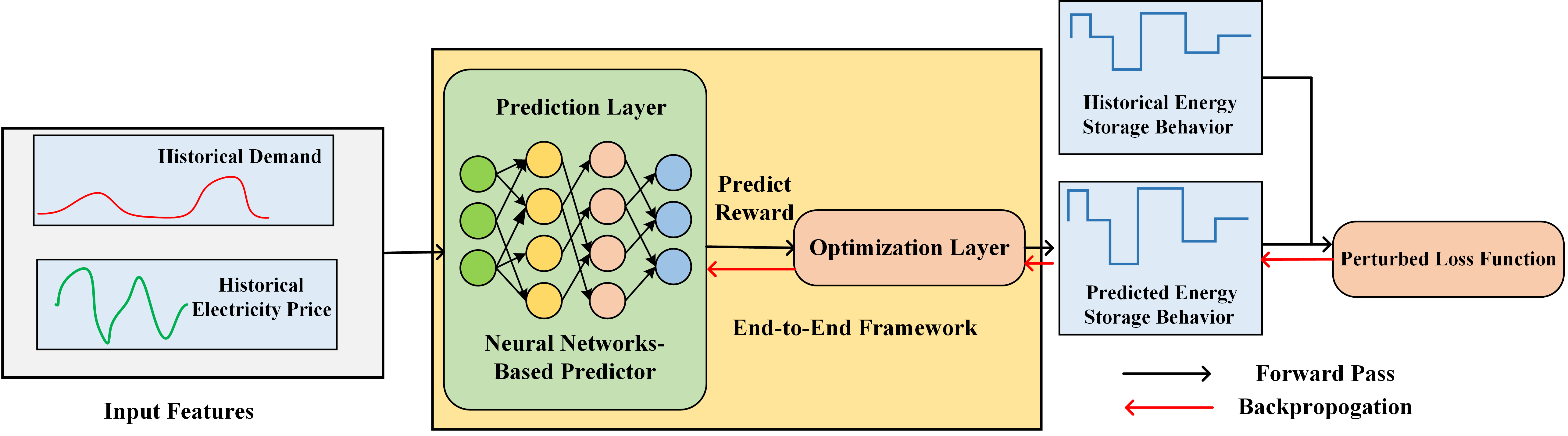
Inspired by the MPC control design used in real-world storage arbitrage controls, our framework consists of two components: the prediction layer and the optimization layer. The prediction layer takes the historical feature as the input and outputs the reward. The pipeline embeds the optimization layer as an additional layer. Therefore, this additional layer must support the forward and backward pass to make it compatible with the prediction layer. The idea of our proposed approach is illustrated in Fig. 1. In the following, we will first detail the prediction layer and the optimization layer and then introduce the learning process.

IV-A The Prediction Layer and the Optimization Layer

Given the input feature $\bm{x}\in\mathbb{R}^{T\times l}$, where $T$ is the length of time series, and $l$ is the number of different types of features. We build the prediction layer based on deep learning neural networks; this layer’s output is the reward prediction. The neural network is parameterized by the weight $\bm{w}$,

$$\hat{\bm{\lambda}}=g_{w}(\bm{x})$$ (3)

where $\hat{\bm{\lambda}}=[\hat{{\lambda}}_{1},\hat{{\lambda}}_{2},...,\hat{{\lambda}}_{T}]^{T}\in\mathbb{R}^{T}$ denotes all rewards $\hat{\lambda}_{t}$ in time horizon $T$. The $g_{w}(.)$ can be any differentiable predictor. In our experiments, we adopt a neural network model as our predictor. As energy storage behaviors strongly correlate with electricity prices and demand, we can include the previous days’ day-ahead price (DAP), real-time price (RTP), and demand data as the input features.

After the hidden reward $\hat{\bm{\lambda}}$ is predicted, the formulation in equation (1) is employed to obtain the storage decisions. The optimization layer $f$ is therefore defined as:

$\displaystyle f:\hat{\bm{\lambda}}\mapsto\underset{{p_{t},b_{t}\in\mathcal{X}}}{\textbf{argmax}}$ $\displaystyle\{\sum_{t=1}^{T}\hat{\lambda}_{t}(p_{t}-b_{t})-u(p_{t},b_{t})\}$ (4)

To simplify the notation, we add additional constraints $y_{t}=p_{t}-b_{t}$ in $\mathcal{X}$ and consider a more general model,

$\displaystyle f:\hat{\bm{\lambda}}\mapsto\underset{{y_{t}\in\mathcal{X}}}{\textbf{argmax}}$ $\displaystyle\{\sum_{t=1}^{T}\hat{\lambda}_{t}y_{t}-u(y_{t})\}=\underset{{\bm{y}\in\mathcal{X}}}{\textbf{argmax}}\,\{\hat{\bm{\lambda}}^{T}\bm{y}-u(\bm{y})\}$ (5)

where $\bm{y}=[y_{1},y_{2},...,y_{T}]^{T}\in\mathbb{R}^{T}$ represents the charge and discharge decisions $(p_{t},b_{t}),t=1,2,...,T$. $u(\bm{y})$ denotes the total cost: $u(\bm{y})=\sum_{t=1}^{T}u(y_{t})$. Specifically, the maximization problem is defined as $F(\hat{\bm{\lambda}})=\underset{{\bm{y}\in\mathcal{X}}}{\textbf{max}}\,\{\hat{\bm{\lambda}}^{T}\bm{y}-u(\bm{y})\}$ and the corresponding optimal solution is $\bm{y}^{*}(\hat{\bm{\lambda}})=\underset{{\bm{y}\in\mathcal{X}}}{\textbf{argmax}}\,\{\hat{\bm{\lambda}}^{T}\bm{y}-u(\bm{y})\}$. Then the end-to-end policy which maps the input features to the energy storage behaviors is defined as:

$$\bm{x}\mapsto\bm{y}=f(g_{w}(\bm{x}))$$ (6)

IV-B The Learning Approach

To ensure good performance with the proposed algorithm, it is crucial to compute the weights of the predictor in a manner that aligns the prediction $\bm{y}$ close to the target energy storage decision $\bar{\bm{y}}$. The learning approach involves training a decision-focused end-to-end framework to follow the decisions taken by an unknown policy.

Dataset. Our learning problem is in a supervised setting and we build a dataset as follows,

$$\mathcal{D}=\{(\bm{x}^{1},\bar{\bm{y}}^{1}),(\bm{x}^{2},\bar{\bm{y}}^{2}),...,(\bm{x}^{n},\bar{\bm{y}}^{n})\}$$ (7)

where $\bm{x}$ denotes the input features, and $\bm{x}$ includes historical price and/or demand data. $\bar{\bm{y}}$ denotes the target energy storage decisions. $n$ is the number of data samples in the dataset. For the energy storage arbitrage problem, $\{\bar{\bm{y}}^{1},\bar{\bm{y}}^{2},...,\bar{\bm{y}}^{n}\}$ represents the optimal arbitrage decisions generated from historical real-time prices. For the behavior prediction problem, $\{\bar{\bm{y}}^{1},\bar{\bm{y}}^{2},...,\bar{\bm{y}}^{n}\}$ represents the historical observed energy storage behaviors.

In order to achieve optimal performance of the prediction of energy storage decisions, it is essential to design an efficient loss function to update the weights $\bm{w}$ of the neural network. This ensures that the prediction of energy storage decisions aligns closely with the target storage decisions.

Learning problem. The learning problem is to find the optimal $\bm{w}^{*}$ such that the loss function $\mathcal{L}(.)$ is minimized over the training dataset $\mathcal{D}$.

$\displaystyle\bm{w}^{*}=\underset{\bm{w}}{\textbf{argmin}}$ $\displaystyle\sum_{i=1}^{n}\mathcal{L}(g_{w}(\bm{x}^{i}),\bar{\bm{y}}^{i})$ (8)

To ensure the prediction follows the target energy storage decisions, it is natural to define a decision-focused loss function such that the computed charge/discharge decisions result in the same profit as the target decisions. Then given estimated reward $\hat{\bm{\lambda}}$, the target charge and discharge decisions $\bar{\bm{y}}$, the decision-focused loss function is defined as

$\displaystyle\mathcal{L}^{FY}(\hat{\bm{\lambda}},\bar{\bm{y}})$ $\displaystyle=\underset{{\bm{y}\in\mathcal{X}}}{\textbf{max}}\,\{\hat{\bm{\lambda}}^{T}\bm{y}-u(\bm{y})\}-(\hat{\bm{\lambda}}\bar{\bm{y}}-u(\bar{\bm{y}}))$ (9)
$\displaystyle=\{\hat{\bm{\lambda}}^{T}\bm{y}^{*}(\hat{\bm{\lambda}})-u(\bm{y}^{*}(\hat{\bm{\lambda}}))\}-(\hat{\bm{\lambda}}\bar{\bm{y}}-u(\bar{\bm{y}}))$

where $\bar{\bm{y}}$ represents the set of target charge and discharge decisions $y_{t},t=1,2,...,T$. It is clear that $\mathcal{L}^{FY}(\hat{\bm{\lambda}},\bar{\bm{y}})\geq 0$ as $\bm{y}^{*}(\hat{\bm{\lambda}})$ is the maximizer given $\hat{\bm{\lambda}}$. The equality $\mathcal{L}^{FY}(\hat{\bm{\lambda}},\bar{\bm{y}})=0$ holds only when $\bm{y}^{*}(\hat{\bm{\lambda}})=\bar{\bm{y}}$. Unfortunately, the loss function in (9) is not continuous because $\bm{y}^{*}(\hat{\bm{\lambda}})$ may not be continuous in $\hat{\bm{\lambda}}$[24][27]. The discontinuity poses computation difficulties when applying backpropagation to update the weights. We employ the perturbation idea in reference [27] by perturbing the reward $\hat{\bm{\lambda}}$ with additive noise. Then the perturbed optimizer is:

$\displaystyle f_{\epsilon}:\hat{\bm{\lambda}}\rightarrow\mathbb{E}[\underset{{\bm{y}\in\mathcal{X}}}{\textbf{argmax}}$ $\displaystyle(\hat{\bm{\lambda}}+\epsilon\bm{Z})^{T}\bm{y}-u(\bm{y})]$ (10)

where $\bm{Z}$ is additive Gaussian noise $\mathcal{N}(\bm{0},\bm{I})$. $\epsilon$ is a positive scaling parameter. $\mathbb{E}[.]$ denotes taking the expectation over the variable $\bm{Z}$. The perturbed maximization problem is defined as $F_{\epsilon}(\hat{\bm{\lambda}})=\mathbb{E}[\underset{{\bm{y}\in\mathcal{X}}}{\textbf{max}}(\hat{\bm{\lambda}}+\epsilon\bm{Z})^{T}\bm{y}-u(\bm{y})]$, and the corresponding optimal solution is $\bm{y}_{\epsilon}^{*}(\hat{\bm{\lambda}})=\mathbb{E}[\underset{{\bm{y}\in\mathcal{X}}}{\textbf{argmax}}(\hat{\bm{\lambda}}+\epsilon\bm{Z})^{T}\bm{y}-u(\bm{y})]$. Thus, the perturbed loss function is defined as:

$\begin{aligned} &\mathcal{L}_{\epsilon}^{PFY}(\hat{\bm{\lambda}},\bar{\bm{y}})=\mathbb{E}[\underset{\bm{y}\in\mathcal{X}}{\textbf{max}}\{(\hat{\bm{\lambda}}+\epsilon\bm{Z})^{T}\bm{y}-u(\bm{y})\}]-(\hat{\bm{\lambda}}^{T}\bar{\bm{y}}-u(\bar{\bm{y}}))\\ \end{aligned}$

(11)

IV-C Convex and Smooth Perturbed Loss Function

We will show in the following Propositions that the perturbed loss function is both convex and smooth, which would facilitate efficient training in the learning pipeline. Our work is motivated by recent work [27]. Due to the space limit, we provide detailed proofs to all propositions in the Appendix.

Proposition 1.

The differentiablity of perturbed function. As noise $\bm{Z}$ is from Gaussian distribution, it has the density $\rho(\bm{Z})\propto\text{exp}(-\psi(\bm{Z}))$. For $\mathcal{R}_{\mathcal{X}}=\underset{{y\in\mathcal{X}}}{\text{max}}||\bm{y}_{\epsilon}^{*}(\hat{\bm{\lambda}})||$, we have

  • $F_{\epsilon}(\hat{\bm{\lambda}})$ is differentiable, and $\nabla_{\hat{\bm{\lambda}}}F_{\epsilon}(\hat{\bm{\lambda}})=\bm{y}_{\epsilon}^{*}(\hat{\bm{\lambda}})=\mathbb{E}[y^{*}(\hat{\bm{\lambda}}+\epsilon\bm{Z})]=\mathbb{E}[F(\hat{\bm{\lambda}}+\epsilon\bm{Z})\nabla_{Z}\psi(\bm{Z})/\epsilon]$.

  • $F_{\epsilon}(\hat{\bm{\lambda}})$ is Lipschitz continuous, and $||F_{\epsilon}(\hat{\bm{\lambda}})-F_{\epsilon}(\tilde{\bm{\lambda}})||\leq\mathcal{R}_{\mathcal{X}}||\hat{\bm{\lambda}}-\tilde{\bm{\lambda}}||.$

where $\propto$ denotes “proportional to.” Proposition 1 proves that $F_{\epsilon}(\hat{\bm{\lambda}})$ is differentiable and Lipschitz continuous, we demonstrate that by adding appropriate Gaussian noise $\bm{Z}$, the perturbed function becomes differentiable with respect to $\hat{\bm{\lambda}}$. The equations from the first statement of Proposition 1 will be used in subsequent proofs. The Lipschitz continuity of $F_{\epsilon}(\hat{\bm{\lambda}})$ helps establish the Lipschitz continuity of ${\nabla\mathcal{L}_{\epsilon}^{PFY}(\hat{\bm{\lambda}},\bar{\bm{y}})}$ in Proposition 4. Given the perturbation, we aim to understand the impact of $\epsilon$ and how the optimal solution $\bm{y}_{\epsilon}^{*}(\hat{\bm{\lambda}})$ behaves as $\epsilon$ varies. Consequently, we introduce Proposition 2:

Proposition 2.

Impact of scaling factor $\epsilon$.

  • $\bm{y}_{\epsilon}^{*}(\hat{\bm{\lambda}})$ is in the interior of $\mathcal{X}$.

  • For $\hat{\bm{\lambda}}$ such that $\bm{y}^{*}({\hat{\bm{\lambda}}})$ is a unique maximizer: when $\epsilon\rightarrow\infty$, $\bm{y}_{\epsilon}^{*}(\hat{\bm{\lambda}})\rightarrow\bm{y}_{1}^{*}(\frac{\hat{\bm{\lambda}}}{\epsilon})=\epsilon\mathbb{E}[\underset{{\bm{y}\in\mathcal{X}}}{\textbf{argmax}}\{\bm{Z}^{T}\bm{y}\}]$; when $\epsilon\rightarrow 0$, $\bm{y}_{\epsilon}^{*}(\hat{\bm{\lambda}})\rightarrow\bm{y}^{*}({\hat{\bm{\lambda}}}).$

Proposition 2 indicates that the perturbed solution $\bm{y}_{\epsilon}^{*}({\hat{\bm{\lambda}}})$ remains feasible. If $\bm{y}^{*}({\hat{\bm{\lambda}}})$ is a unique maximizer, as $\epsilon\rightarrow 0$, $\bm{y}_{\epsilon}^{*}(\hat{\bm{\lambda}})$ converges to the original optimal solution $\bm{y}^{*}({\hat{\bm{\lambda}}})$. Conversely, as $\epsilon\rightarrow\infty$, $\bm{y}_{\epsilon}^{*}(\hat{\bm{\lambda}})$ deviates from the original solution $\bm{y}^{*}({\hat{\bm{\lambda}}})$ and approaches $\bm{y}_{1}^{*}(\frac{\hat{\bm{\lambda}}}{\epsilon})$. Since $\bm{Z}$ is drawn from a zero-mean Gaussian distribution, $\bm{y}_{1}^{*}(\frac{\hat{\bm{\lambda}}}{\epsilon})$ converges to a zero vector. In the context of our energy storage model, as $\epsilon$ tends to infinity, it implies that the energy storage system remains inactive and does not take any action.

This proposition implies that we should carefully select the scaling factor $\epsilon$. A very small $\epsilon$ may not ensure sufficient smoothness of the loss function, while a very large $\epsilon$ may cause the solution to deviate significantly from the original optimal solution. In our experimental setup, $\epsilon$ is set between 1 and 10.

Proposition 3.

The property of perturbed loss function $\mathcal{L}_{\epsilon}^{PFY}(\hat{\bm{\lambda}},\bar{\bm{y}})$.

  • $\mathcal{L}_{\epsilon}^{PFY}(\hat{\bm{\lambda}},\bar{\bm{y}})$ is a convex function of ${\hat{\bm{\lambda}}}$.

  • $0\leq\mathcal{L}_{\epsilon}^{PFY}(\hat{\bm{\lambda}},\bar{\bm{y}})-\mathcal{L}^{FY}(\hat{\bm{\lambda}},\bar{\bm{y}})\leq TP\epsilon$.

where $T$ represents the length of the prediction horizon, and $P$ represents the power rating. The left inequality in the second statement implies that the perturbed loss function serves as an upper bound for the original loss function, $\mathcal{L}^{FY}(\hat{\bm{\lambda}},\bar{\bm{y}})\leq\mathcal{L}_{\epsilon}^{PFY}(\hat{\bm{\lambda}},\bar{\bm{y}})$. The right inequality indicates that the distance between these two loss functions is bounded by the scaling factor $\epsilon$. As $\epsilon\rightarrow 0$, these two inequalities together imply the convergence $\mathcal{L}_{\epsilon}^{PFY}(\hat{\bm{\lambda}},\bar{\bm{y}})\rightarrow\mathcal{L}^{FY}(\hat{\bm{\lambda}},\bar{\bm{y}})$.

Proposition 4.

Gradient of perturbed loss function.

  • The gradient of the perturbed loss function is

    $\displaystyle{\nabla\mathcal{L}_{\epsilon}^{PFY}(\hat{\bm{\lambda}},\bar{\bm{y}})}=\bm{y}_{\epsilon}^{*}(\hat{\bm{\lambda}})-\bar{\bm{y}}.$ (12)
  • ${\nabla\mathcal{L}_{\epsilon}^{PFY}(\hat{\bm{\lambda}},\bar{\bm{y}})}$ is Lipschitz continuous.

(12)italic-(12italic-)\eqref{eq: prop4} shows that the perturbed loss function has a convenient gradient, which can be computed by solving for the optimal solution and subtracting $\bar{\bm{y}}$. Lipschitz continuity ensures that the gradient changes smoothly, which is beneficial for training the learning problem. Hence, we have shown that the perturbed loss function is both convex and smooth.

Convergence Analysis of the Optimization Layer: As shown in later equation (17), the total gradient with respect to the network weights $\bm{w}$ relies on the chain rule. However, conducting a comprehensive convergence analysis is beyond the scope of this paper as it requires several assumptions regarding neural networks to complete the proof. Without loss of generality, we focus on the perturbed optimization layer and consider $\mathcal{L}_{\epsilon}^{PFY}(\hat{\bm{\lambda}},\bar{\bm{y}})$ as a function of $\hat{\bm{\lambda}}$. Given that $\mathcal{L}_{\epsilon}^{PFY}(\hat{\bm{\lambda}},\bar{\bm{y}})$ is a convex function of ${\hat{\bm{\lambda}}}$ in Proposition 3, and ${\nabla\mathcal{L}_{\epsilon}^{PFY}(\hat{\bm{\lambda}},\bar{\bm{y}})}$ is Lipschitz continuous in Proposition 4, we provide a convergence analysis for the optimization layer in Appendix.

IV-D Algorithmic Implementation

Since the exact computation of the expectation in (11) is generally intractable, we approximate it using Monte Carlo sampling in the solution algorithm implementation. The perturbed loss function is approximated as:

$\displaystyle\mathcal{L}_{\epsilon}^{PFY}(\hat{\bm{\lambda}},\bar{\bm{y}})$ (13)
$\displaystyle\approx\frac{1}{K}\sum_{m=1}^{K}[\underset{\bm{y}\in\mathcal{X}}{\textbf{max}}\{(\hat{\bm{\lambda}}+\epsilon\bm{Z}^{(m)})^{T}\bm{y}-u({\bm{y}})\}]-(\hat{\bm{\lambda}}^{T}\bar{\bm{y}}-u(\bar{\bm{y}}))$

where $K$ is the number of Monte-Carlo samples. The gradient ${\nabla\mathcal{L}_{\epsilon}^{PFY}(\hat{\bm{\lambda}},\bar{\bm{y}})}$ is computed as follows:

$\displaystyle{\nabla\mathcal{L}_{\epsilon}^{PFY}(\hat{\bm{\lambda}},\bar{\bm{y}})}=\bm{y}_{\epsilon}^{*}(\hat{\bm{\lambda}})-\bar{\bm{y}}$ (14)
$\displaystyle=\mathbb{E}[\underset{\bm{y}\in\mathcal{X}}{\textbf{argmax}}(\hat{\bm{\lambda}}+\epsilon\bm{Z})^{T}\bm{y}-u(\bm{y})]-\bar{\bm{y}}$
$\displaystyle\approx\frac{1}{K}\sum_{m=1}^{K}[\underset{{\bm{y}\in\mathcal{X}}}{\textbf{argmax}}(\hat{\bm{\lambda}}+\epsilon\bm{Z}^{(m)})^{T}\bm{y}-u(\bm{y})]-\bar{\bm{y}}$

Given that the unknown predictor is designed to forecast real-time prices, we can guide the inferred reward to align with the price information by leveraging it as prior knowledge. To achieve this, we introduce a predictor regularizer, which minimizes the mean squared error (MSE) between the reward and the price. The price data may consist of either previous days’ real-time prices or day-ahead prices. Consequently, the total loss function is constructed as the weighted sum of the perturbed loss $\mathcal{L}^{PFY}_{\epsilon}(\hat{\bm{\lambda}},\bar{\bm{y}})$ and the MSE loss. This hybrid loss function is defined as:

$$\mathcal{L}_{\epsilon}(\hat{\bm{\lambda}},\bar{\bm{y}})=\mathcal{L}^{PFY}_{\epsilon}(\hat{\bm{\lambda}},\bar{\bm{y}})+\beta\sum_{t=1}^{T}(\hat{\lambda}_{t}-\xi_{t})^{2}$$ (15)

The parameter $\beta$ represents the weighted factor of the MSE loss, and $\xi_{t}$ corresponds to the RTP or DAP from the previous day, serving as one of the features in $x_{t}$. The total subgradient is then computed as:

$\displaystyle{\nabla\mathcal{L}_{\epsilon}(\hat{\bm{\lambda}},\bar{\bm{y}})}=\bm{y}_{\epsilon}^{*}(\hat{\bm{\lambda}})-\bar{\bm{y}}+2\beta(\hat{\bm{\lambda}}-\bm{\xi})$ (16)
$\displaystyle\approx\frac{1}{K}\sum_{m=1}^{K}[\underset{{\bm{y}\in\mathcal{X}}}{\textbf{argmax}}(\hat{\bm{\lambda}}+\epsilon\bm{Z}^{(m)})^{T}\bm{y}-u(\bm{y})]-\bar{\bm{y}}+$
$\displaystyle 2\beta(\hat{\bm{\lambda}}-\bm{\xi})$

For the backward propagation, we apply the chain rule to compute the total gradient with respect to the weights $\bm{w}$ of predictors,

$${\nabla_{\bm{w}}\mathcal{L}_{\epsilon}(\hat{\bm{\lambda}},\bar{\bm{y}})}={\nabla\mathcal{L}_{\epsilon}(\hat{\bm{\lambda}},\bar{\bm{y}})}\cdot\frac{\partial\hat{\bm{\lambda}}}{\partial\bm{w}}$$ (17)

where the term $\frac{\partial\hat{\bm{\lambda}}}{\partial\bm{w}}$ represents the Jacobian of reward prediction with respect to the weights $\bm{w}$. The Jacobian can be computed using automatic differentiation [28] in a standard deep learning framework. The details of behavior prediction are outlined in Algorithm 1. The energy storage arbitrage follows a similar process as described in Algorithm 2. Due to space limitations, Algorithm 2 is moved to the Appendix. Readers can refer to the Appendix for more details.

Algorithm 1 The Prediction of Strategic Energy Storage Behavior
0:  The time horizon $T$; The power rating $P$ of energy storage; The SoC efficiency $\eta$ and capacity $E$; The maximum epochs $M_{\max}$; The cost coefficients in $u(p_{t},b_{t})$; The training data $\mathcal{D}=\{(\bm{x}^{1},\bar{\bm{y}}^{1}),(\bm{x}^{2},\bar{\bm{y}}^{2}),...,(\bm{x}^{n},\bar{\bm{y}}^{n})\}$; The testing data $\hat{\mathcal{D}}=\{\hat{\bm{x}}^{1},\hat{\bm{x}}^{2},...,\hat{\bm{x}}^{n}\}$.
1:  Initialization: The weights $\bm{w}$ of predictor $g_{w}(\bm{x})$ are randomly initialized.Training stage:
2:  for Epochs < $M_{\max}$  do
3:     for Each batch in $\mathcal{D}$  do
4:        Predict the reward using the predictor $\hat{\bm{\lambda}}=g_{w}(\bm{x})$;
5:        Forward pass to compute the optimal decisions $p_{t}^{*},b_{t}^{*},t=1,2,...,T$ by equation (1);
6:        Compute the loss $\mathcal{L}_{\epsilon}(\hat{\bm{\lambda}},\bar{\bm{y}})$ by equation (15);
7:        Compute the total gradient by equation (17) and backward pass to update the weights $\bm{w}$ of predictor.;
8:     end for
9:  end forPrediction stage:
10:  Predict the reward using the predictor $\hat{\bm{\lambda}}=g_{w}(\hat{\bm{x}})$;
11:  Forward pass to compute the optimal decisions $\hat{p}_{t},\hat{b}_{t},t=1,2,...,T$ by equation (1);
12:  return  The predicted energy storage behaviors $(\hat{p}_{t},\hat{b}_{t})$ for $t=1,2,...T$.

V Experiments

The experiments are implemented in Python 3, Pytorch [29] and PyEPO package [30] on a desktop with 3.0 GHz Intel Core i9, NVIDIA 4080 16 GB Graphic card, and 32 GB RAM. The optimization layer is implemented using the Groubi optimization package [31]. The pre-built predictor is implemented in Keras [32] and Tensorflow [33].

The parameters for the energy storage arbitrage model are set as follows: power rating $P=0.5MW$, storage efficiency $\eta=0.9$, initial SoC $e_{0}=0.5MWh$, storage capacity $E=2MWh$, prediction horizon $T=24$. The number of Monte-Carlo samples is $K=1$.

V-A Self-Scheduling Energy Storage Arbitrage

We conduct experiments focusing on Behind-the-Meter energy storage arbitrage, where the energy storage system autonomously manages its scheduling based on future price predictions at hourly real-time prices [12]. The reward forecasting horizon spans 24 hours and is updated hourly. Therefore, the corresponding energy storage schedule is dynamically adjusted on an hourly basis. We use price data from the New York Independent System Operator (NYISO), using data from 2017-2020 for training and 2021 data for testing. The arbitrage profit is computed as

$$\textstyle\sum_{t=1}^{T}\bar{\lambda}_{t}(p_{t}^{*}-b_{t}^{*})-u(p^{*}_{t},b_{t}^{*})$$ (18)

where $\bar{\lambda}_{t}$ denotes the real-time price at time $t$; $p_{t}^{*}$ and $b_{t}^{*}$ denote the scheduled discharge and charge at time $t$, respectively.

Refer to caption
Refer to caption
Figure 2: Comparison of annual accumulative profits between the proposed approach and two benchmark methods. The energy storage model is with (a)linear cost term, (b)linear and quadratic cost terms.

We employ the Multi-Layer Perceptron (MLP) as our prediction layer. We compare the arbitrage performance of the proposed method with two MPC-based benchmark methods. The first benchmark employs a Long Short-Term Memory (LSTM) network for real-time price prediction, while the second employs an MLP network. For brevity, we denote these two methods as “LSTM-MPC” and “MLP-MPC”, respectively. We test two types of energy storage models to evaluate the performance of our proposed method: one with a linear cost term and the other with both linear and quadratic cost terms. The linear cost term is $u(p_{t},b_{t})=C_{1}p_{t}$, where the coefficient of discharge cost is $C_{1}=10$. The linear and quadratic cost terms are $u(p_{t},b_{t})=C_{1}p_{t}+C_{2}p_{t}^{2}$, where the coefficients of discharge cost are $C_{1}=5$ and $C_{2}=5$.

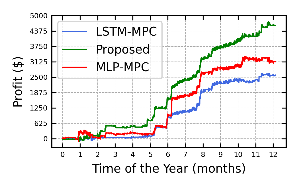
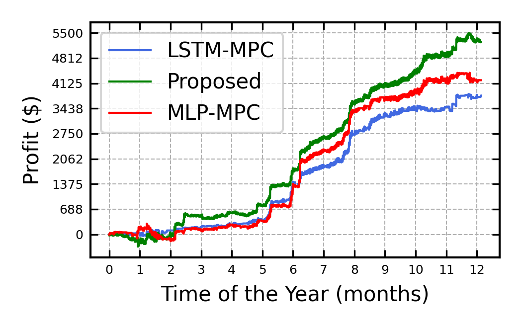
Note that the self-scheduling energy storage arbitrage setting in this paper is more challenging than the economic bidding or price response settings in [9]. Economic bidding assumes that energy storage can submit a bid, and the market clears it based on the price at time $t$. Price response assumes that the price at the time step $t$ can be observed before making decisions at $t$. However, self-scheduling arbitrage in this paper requires making decisions at $t$ before the real-time price at $t$ is published. Consequently, this self-scheduling setting encounters more uncertainties and leads to lower profits than the other two settings. The accumulative arbitrage profits are plotted on a yearly basis.

Fig. 2 shows the arbitrage performance of the proposed method and the two benchmark methods with the two considered cost terms. The mean absolute error (MAE) of the MLP model is 10.83, while the MAE of the LSTM model is 9.31. Although the lower MAE of the LSTM indicates better overall prediction accuracy compared to the MLP, the MLP model performs better in terms of profit. This is because the MLP predicts the price peak timing more accurately, a crucial factor for optimizing energy storage arbitrage. The proposed method consistently outperforms the two benchmark methods. Our proposed method demonstrates a performance improvement of approximately $47\%$ and $77\%$ over the two benchmark methods with linear cost and 25% and 39% with linear and quadratic cost. Our end-to-end pipeline, which incorporates the optimization model and focuses on decision error, contributes to its profit improvement. The results in the two sub-figures also demonstrate that our proposed method is robust across different energy storage cost models.

We vary the energy storage efficiency and show the corresponding profits in Table I. The profits decrease as the efficiency decreases for all three methods. The proposed method achieves 5%-20% profit improvement over the two benchmark methods when $\eta=1$. In contrast, for $\eta=0.85$, the profits of the proposed method are more than double those of the two benchmark methods. Unlike the two benchmark methods, which treat prediction and optimization as two separate stages, the proposed method incorporates the SoC evolution into the end-to-end pipeline. The results in Table I demonstrate that the proposed method is more robust to varying storage efficiencies, highlighting its superiority.

Table I: The comparison of accumulative profits with different energy storage efficiency with linear cost.
$\eta$ 1 0.95 0.9 0.85
Proposed 8809 6381 4589 2990
MLP-MPC 8430 5545 3121 1332
LSTM-MPC 7248 4554 2583 1233

V-B Energy Storage Behavior Prediction

The prediction of energy storage behavior involves predicting the charge and discharge patterns of an energy storage unit based on observed energy storage actions and input features. To evaluate the performance of our proposed algorithm, we compared it with two benchmark prediction methods. The first benchmark algorithm trains an LSTM network to learn a nonlinear mapping between input features and charge/discharge decisions. This mapping resembles the one in (6) but removes the optimization layer. It can be expressed as,

$$\bm{x}\mapsto\bm{y}=g_{w}(\bm{x})$$ (19)

We denote the first algorithm as its neural network type “LSTM” for brevity. The second algorithm is a two-stage approach and assumes a pre-built predictor. After predicting real-time price, the price predictions are fed into the storage optimization problem defined in equation (1). Due to its two-stage nature, we abbreviate this method as “Two-Stage.”

Evaluation Metric. We employ principles of pattern recognition to assess the efficacy of storage behavior prediction models [34]. Our motivation stems from the unique characteristics of storage operations, which are inherently bi-directional—alternating between charging and discharging phases—and marked by the action’s sparsity, where the output of the storage remains at zero for extended durations. Traditional evaluation metrics, including mean-square error and correlation coefficients, fall short of accurately capturing the prediction quality due to these distinct operational dynamics.

We assign the label 1 to the discharge decision, -1 to the charge decision, and 0 to the standby decision. Predicted values are classified as 1 if above the threshold, -1 if below the negative threshold, and 0 if within the range between the negative threshold and the threshold. The threshold is set at 10%-20% of the power rating. In the synthetic experiment, we set the threshold to 0.05; in the real-world experiment, we set it to 0.2. We consider the time delays, and if the prediction and the ground truth differ by at most 2 hours, we still consider it correctly classified. The confusion matrix with this criterion is denoted as the “event-based confusion matrix.” The confusion matrix is defined in Table II, where TP is true positive; TN is true negative; FN is false negative; FP is false positive.

Table II: The confusion matrix of energy storage behavior.
Actual | Prediction -1 0 1
-1 TP FN FP
0 FP TN FP
1 FP FN TP

Due to the event-based criterion not considering the magnitude of the prediction, we also introduce a magnitude-based criterion: if the prediction error for charge/discharge falls within a certain percentage of magnitude of the actual value, it is classified as 1 or -1, respectively; otherwise, it is labeled as 0. In the synthetic experiment, we set the percentage at 20%; in the real-world experiment, we set it at 40%. The time delays are also accounted for in the magnitude-based criterion. We denote the confusion matrix with this criterion as the “magnitude-based confusion matrix.” The evaluation metrics are defined as:

Precision $\displaystyle=\mathrm{\frac{TP}{TP+FP}}$ (20a)
Accuracy $\displaystyle=\mathrm{\frac{TP+TN}{TP+TN+FP+FN}}$ (20b)
Recall $\displaystyle=\mathrm{\frac{TP}{TP+FN}}$ (20c)
F1 score $\displaystyle=\mathrm{\frac{2\times Precision\times Recall}{Precision+Recall}}$ (20d)

V-B1 Storage Behavior Prediction with Synthetic Data

The historical data of RTP, DAP, and demand data are collected from NYISO within the New York City load zone from 2019 to 2022. These historical data are used as the input features for the proposed and benchmark methods. We use two years for training and one year for testing. The data resolution is one sample per hour. We employ an LSTM network as our prediction layer. The energy storage arbitrage model in (1) generates the energy storage behaviors. The governing reward, i.e., the synthetic price prediction, $\hat{\bm{\lambda}}\in\mathbb{R}^{T}$ is generated by:

$$\hat{\lambda}^{g}_{i,t}=\alpha_{i,t}*\lambda^{DA}_{i,t}+(1-\alpha_{i,t})*\lambda^{RT}_{i,t}+\zeta_{i,t}$$ (21)

where $\lambda^{DA}_{i,t}$ and $\lambda^{RT}_{i,t}$ represent the DAP and RTP at time step $t$ of day $i$, respectively. $\zeta_{i,t}$ is the Gaussian noise generated from $\mathcal{N}(0,1)$. $\alpha_{i,t}$ is the parameter that controls the trade-off similarity between DAP and RTP. Note that this reward generation method is motivated by the fact that the expectation of RAP converges to DAP [35]. We randomly select $\alpha_{i,t}$ from (0.5,1) in our experiment. The two-stage method constructs a predictor for RTP based on the same historical data and then incorporates the prediction into the arbitrage model.

Refer to caption
Figure 3: Comparison of ground-truth and predictions from the proposed approach and two benchmark methods: storage model with linear cost.

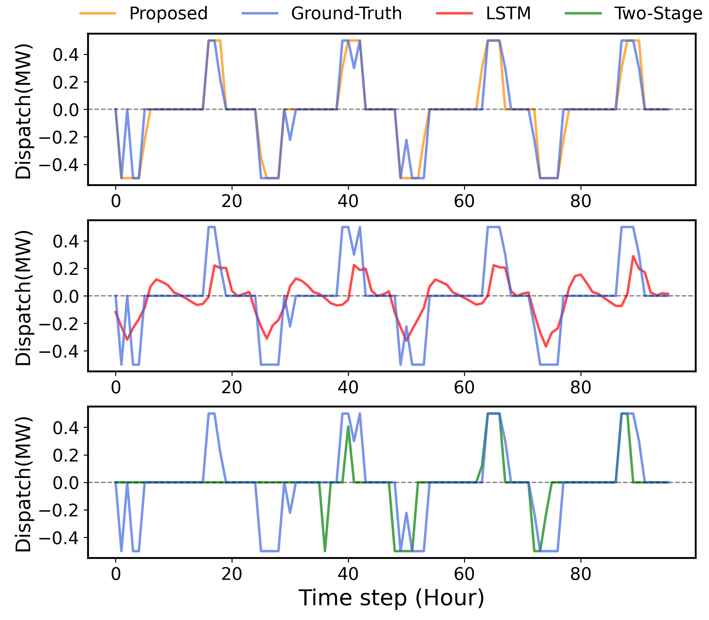
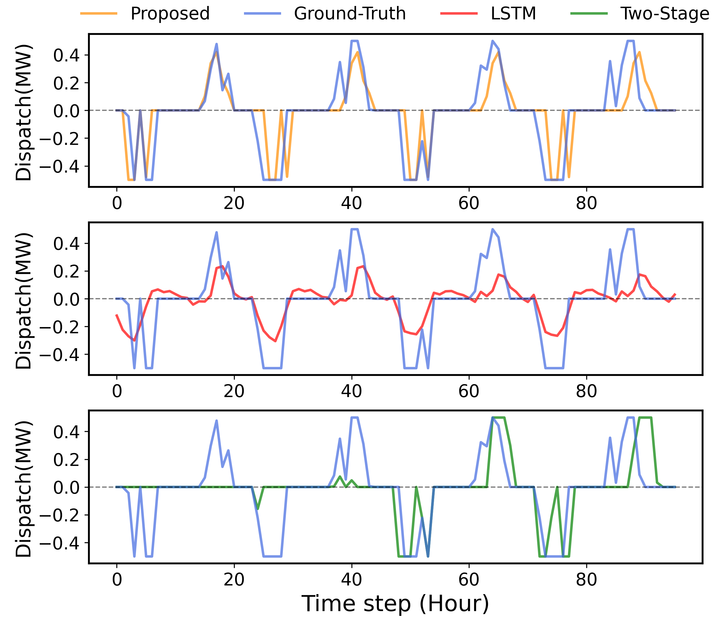
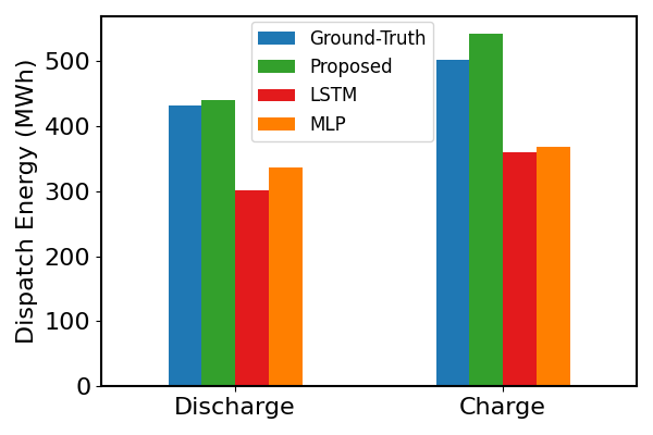
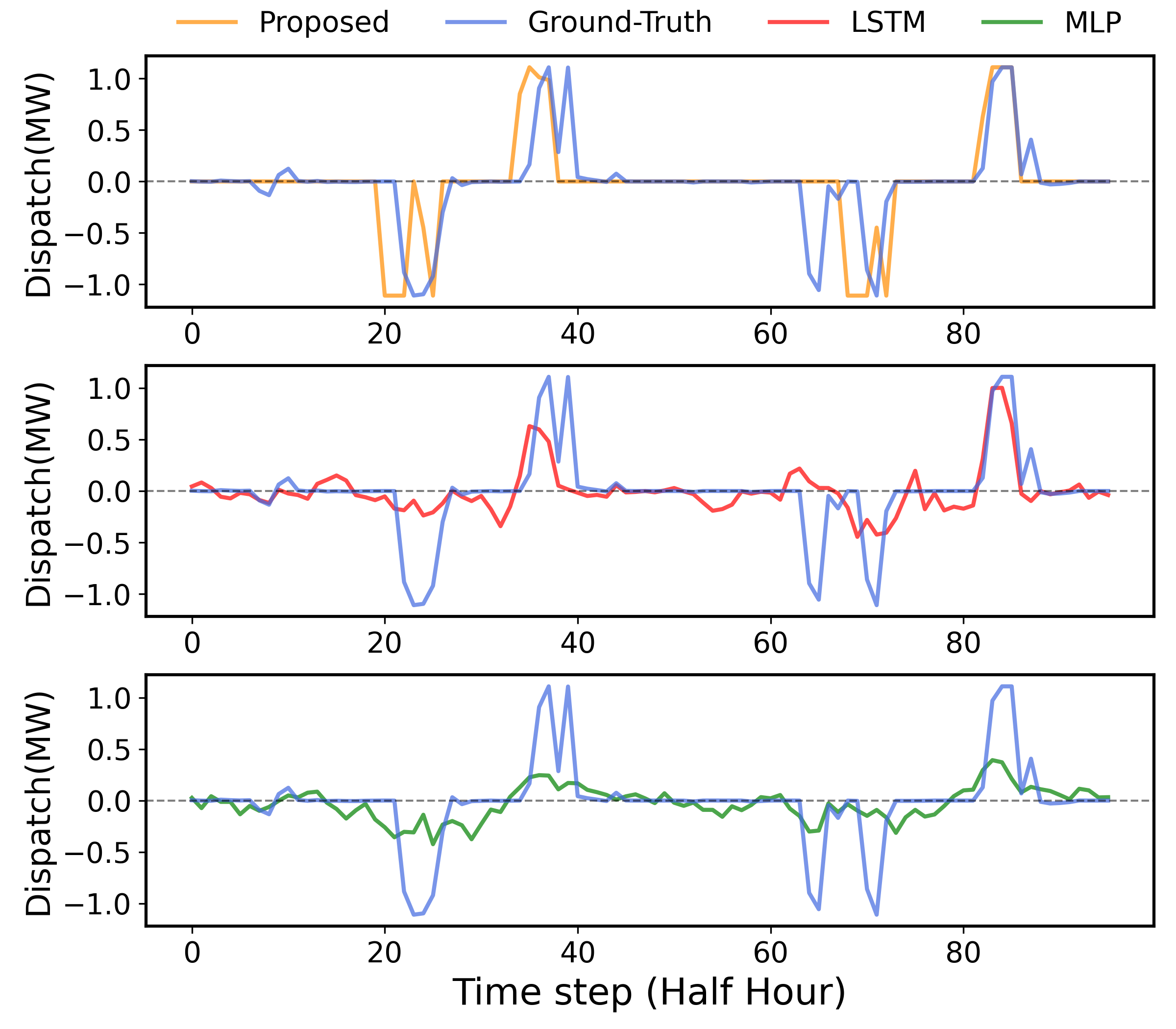
We evaluate the performance of our proposed method using energy storage models with two cost terms. The settings for these cost terms are consistent with those described in Section V-A. The hyperparameter $\beta$ is set as $\beta=0.001$. Fig. 3 and Fig. 4 show the prediction performance of the proposed method and two benchmark methods. The ground-truth behaviors and the predictions in four consecutive days are plotted. The proposed method accurately predicts storage behaviors regarding time steps and magnitudes. In contrast, the LSTM method can predict the timing of charge/discharge decisions but struggles to learn power rating information from historical data. Additionally, it mispredicts charge/discharge behaviors during standby periods when energy storage remains inactive. The two-stage method can capture the power rating but predicts a shorter duration. Additionally, it fails to predict energy storage activities on the first two days because the pre-built predictor underestimates the price spread, leading the model to stay on standby.

Refer to caption
Figure 4: Comparison of ground-truth and predictions from the proposed approach and two benchmark methods: storage model with linear and quadratic cost.

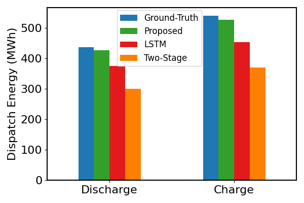
The total dispatch energy of ground-truth, the proposed method and two comparison methods is shown in Fig. 5(a) and (b). Our proposed method accurately predicts the charge and discharge energy while the two benchmark methods have higher errors. This demonstrates the superiority of our approach.

Table III and Table IV list the number of True Positives (TP), True Negatives (TN), False Positives (FP), and False Negatives (FN) along with two types of confusion matrices. The event-based confusion matrix shows that the proposed method achieves the highest precision and accuracy. While the proposed method has lower recall than LSTM, it achieves much higher precision. The F1 score, which balances precision and recall, indicates that our method outperforms others overall. The magnitude-based confusion matrix employs a more strict criterion. In both tables, the performance of the LSTM method degrades significantly under this criterion. In contrast, the F1 score of the proposed method experiences only a marginal decrease. This indicates that the proposed method is more adept at accurately predicting the magnitude. The F1 scores in both tables demonstrate that the proposed method outperforms the other two methods.

Refer to caption
Refer to caption
Refer to caption
Figure 5: Energy dispatch of ground-truth, the proposed approach and two benchmark methods: (a) energy storage model with a linear cost term, (b) energy storage model with linear and quadratic cost terms, and (c) energy storage model based on real-world data.
Table III: Comparison of the proposed approach and two benchmark methods, storage model with linear cost term.
Event-based confusion matrix Magnitude-based confusion matrix
Metrics TP TN FP FN Precision Accuracy Recall F1 score TP TN FP FN Precision Accuracy Recall F1 score
Prop 1463 5878 672 723 68.52% 84.03% 66.93% 67.72% 1235 5808 742 951 62.47% 80.62% 56.50% 59.33%
LSTM 1987 4166 2418 165 45.11% 70.43% 92.33% 60.61% 132 4004 2580 2020 4.87% 47.34% 6.13% 5.43%
Two-Stage 943 6015 548 1230 63.25% 79.65% 43.40% 51.47% 787 6034 529 1386 59.80% 78.08% 36.22% 45.11%
Table IV: Comparison of the proposed approach and two benchmark methods, storage model with linear and quadratic cost term.
Event-based confusion matrix Magnitude-based confusion matrix
Metrics TP TN FP FN Precision Accuracy Recall F1 score TP TN FP FN Precision Accuracy Recall F1 score
Prop 2327 4796 1018 595 69.57% 81.54% 79.64% 74.26% 1252 4944 870 1670 59% 70.92% 42.85% 49.64%
LSTM 2577 3647 2242 270 53.48% 71.25% 90.52% 67.23% 228 3518 2371 2619 8.77% 42.88% 8.01% 8.37%
Two-Stage 1430 5195 629 1482 69.45% 75.84% 49.11% 57.53% 906 5198 626 2006 59.14% 69.87% 31.11% 40.77%
Table V: Comparison of the proposed approach and two benchmark methods on real-world data.
Event-based confusion matrix Magnitude-based confusion matrix
Metrics TP TN FP FN Precision Accuracy Recall F1 score TP TN FP FN Precision Accuracy Recall F1 score
Prop 792 4252 352 364 69.23% 87.57% 68.51% 68.87% 602 4272 332 554 64% 84.62% 52.08% 57.61%
LSTM 609 4297 293 561 67.52% 85.17% 52.05% 58.78% 345 4299 291 825 54.25% 80.62% 29.49% 38.21%
MLP 764 4024 580 392 56.85% 83.12% 66.09% 61.12% 367 4060 544 789 40.29% 76.86% 31.75% 35.51%
Refer to caption
Figure 6: Comparison of ground-truth and predictions from the proposed approach and two benchmark methods: real-world data.

V-B2 Storage Behavior Prediction with Real-World Data

We conduct experiments on public energy storage data from Queensland University. The Tesla Powerpack battery system has a 1.1 MW power rating and a 2.2 MWh capacity. The battery system is controlled by a demand response engine and engages in two major revenue activities: arbitrage and Frequency Control Ancillary Services (FCAS). According to its performance report [36], the battery system only had a 2-hour duration of FCAS in 2020. Therefore, energy storage behaviors are dominated by storage arbitrage. The data resolution is one sample every 30 minutes. Six months of data are used for training, and four months of data are used for testing. Some days did not have charging/discharging activities due to internet connection issues. Historical energy storage behaviors also have missing data issues for several days. These days are removed from the training and testing data. We only include RTP data as input features.

The parameters of the energy storage arbitrage model are set as follows: power rating $P=1.11MW$, storage efficiency $\eta=0.9$, storage capacity $E=2.2MWh$, the prediction horizon $T=96$, we assume the energy storage model has a linear cost term and a quadratic cost term $u(p_{t},b_{t})=C_{1}p_{t}+C_{2}p_{t}^{2}$, where the coefficients of discharge cost is set as $C_{1}=5$, $C_{2}=3$. The hybrid loss parameter $\beta=0.01$. Note that predicting real-world energy storage behaviors is inherently challenging. First, complete knowledge of model parameters, such as prediction horizon and strategy, is unavailable. Second, our algorithm requires the SoC to be consistent across days, but data quality issues lead to some days being excluded, complicating the learning process. The stochastic nature of real-world energy storage adds further difficulty for accurate behavior predictions. Despite all these challenges, our method consistently outperforms the benchmark methods on this real-world dataset.

We compare the proposed method with the first comparison algorithm, using two types of neural networks, LSTM and MLP. Fig. 6 shows the prediction performance of the proposed method and the benchmark methods. The proposed method captures the trend and magnitude in ground-truth energy storage behaviors, albeit with some time deviations. Although the LSTM method predicts discharge decisions well, it consistently fails to predict the magnitude of charge decisions. The MLP method can approximately predict the timing of charge/discharge decisions, but it consistently struggles to predict their magnitude. Hence, the practical applicability of these two methods is highly constrained.

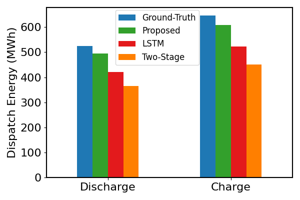
Table V lists the confusion matrices and corresponding metrics. Table V shows that the proposed method achieves the best performance for all metrics. Fig. 5(c) shows the total dispatch energy for the proposed and comparison methods. Our method slightly over-predicts charge and discharge energy, while the two benchmark methods exhibit much higher prediction errors. These results underscore the substantial advantage of the proposed method.

VI Conclusions

This paper introduces a decision-focused approach that integrates the physical energy storage model into a neural network-based architecture. Our method incorporates prior knowledge from the storage arbitrage model and infers the hidden reward that guides energy storage decisions. We provide theoretical analysis for the perturbed loss function. To facilitate effective training, we propose a novel hybrid loss function. We demonstrate our proposed framework on two energy storage applications: the self-scheduling energy storage arbitrage problem and the energy storage behavior prediction problem. Numerical results on both applications underscore the significant advantages of our proposed method. In future work, we plan to explore various neural network architectures and select the best-performing networks for our framework. Additionally, we aim to investigate integrating our method into Behind-the-Meter energy disaggregation of energy storage.

References

  • [1] U. E. I. Administration, “U.s. battery storage capacity expected to nearly double in 2024,” , 2023.
  • [2] S. M. Harvey and W. W. Hogan, “Market power and withholding,” Harvard Univ., Cambridge, MA, 2001.
  • [3] N. Zheng, Q. Xin, W. Di, G. Murtaugh, and B. Xu, “Energy storage state-of-charge market model,” IEEE Transactions on Energy Markets, Policy and Regulation, vol. 1, no. 1, pp. 11–22, 2023.
  • [4] R. Sioshansi, P. Denholm, J. Arteaga, S. Awara, S. Bhattacharjee, A. Botterud, W. Cole, A. Cortes, A. De Queiroz, J. DeCarolis et al., “Energy-storage modeling: State-of-the-art and future research directions,” IEEE transactions on power systems, vol. 37, no. 2, pp. 860–875, 2021.
  • [5] Z. Zhou, N. Zheng, R. Zhang, and B. Xu, “Energy storage market power withholding bounds in real-time markets,” in Proceedings of the 15th ACM International Conference on Future Energy Systems, 2024.
  • [6] L. Sang, Y. Xu, H. Long, Q. Hu, and H. Sun, “Electricity price prediction for energy storage system arbitrage: A decision-focused approach,” IEEE Transactions on Smart Grid, vol. 13, no. 4, pp. 2822–2832, 2022.
  • [7] Y. Wang, Y. Dvorkin, R. Fernández-Blanco, B. Xu, T. Qiu, and D. S. Kirschen, “Look-ahead bidding strategy for energy storage,” IEEE Transactions on Sustainable Energy, vol. 8, no. 3, pp. 1106–1117, 2017.
  • [8] D. R. Jiang and W. B. Powell, “An approximate dynamic programming algorithm for monotone value functions,” Operations research, vol. 63, no. 6, pp. 1489–1511, 2015.
  • [9] Y. Baker, N. Zheng, and B. Xu, “Transferable energy storage bidder,” IEEE Transactions on Power Systems, 2023.
  • [10] D. R. Jiang and W. B. Powell, “Optimal hour-ahead bidding in the real-time electricity market with battery storage using approximate dynamic programming,” INFORMS Journal on Computing, vol. 27, no. 3, pp. 525–543, 2015.
  • [11] K. Abdulla, J. De Hoog, V. Muenzel, F. Suits, K. Steer, A. Wirth, and S. Halgamuge, “Optimal operation of energy storage systems considering forecasts and battery degradation,” IEEE Transactions on Smart Grid, vol. 9, no. 3, pp. 2086–2096, 2016.
  • [12] H. Chitsaz, P. Zamani-Dehkordi, H. Zareipour, and P. P. Parikh, “Electricity price forecasting for operational scheduling of behind-the-meter storage systems,” IEEE Transactions on Smart Grid, vol. 9, no. 6, pp. 6612–6622, 2017.
  • [13] H. Wang and B. Zhang, “Energy storage arbitrage in real-time markets via reinforcement learning,” in 2018 IEEE Power & Energy Society General Meeting (PESGM).   IEEE, 2018, pp. 1–5.
  • [14] N. Zheng, J. Jaworski, and B. Xu, “Arbitraging variable efficiency energy storage using analytical stochastic dynamic programming,” IEEE Transactions on Power Systems, vol. 37, no. 6, pp. 4785–4795, 2022.
  • [15] C. Zhang, Y. Fu, and L. Gong, “Short-term electricity price forecast using frequency analysis and price spikes oversampling,” IEEE Transactions on Power Systems, 2022.
  • [16] X. Lu, J. Qiu, G. Lei, and J. Zhu, “An interval prediction method for day-ahead electricity price in wholesale market considering weather factors,” IEEE Transactions on Power Systems, 2023.
  • [17] S. Liu, C. Wu, and H. Zhu, “Topology-aware graph neural networks for learning feasible and adaptive ac-opf solutions,” IEEE Transactions on Power Systems, 2022.
  • [18] R. Fernández-Blanco, J. M. Morales, and S. Pineda, “Forecasting the price-response of a pool of buildings via homothetic inverse optimization,” Applied Energy, vol. 290, p. 116791, 2021.
  • [19] A. Kovács, “Inverse optimization approach to the identification of electricity consumer models,” Central European Journal of Operations Research, vol. 29, no. 2, pp. 521–537, 2021.
  • [20] T. X. Nghiem and C. N. Jones, “Data-driven demand response modeling and control of buildings with gaussian processes,” in 2017 American Control Conference (ACC).   IEEE, 2017, pp. 2919–2924.
  • [21] J. Vuelvas and F. Ruiz, “A novel incentive-based demand response model for cournot competition in electricity markets,” Energy Systems, vol. 10, no. 1, pp. 95–112, 2019.
  • [22] Y. Bian, N. Zheng, Y. Zheng, B. Xu, and Y. Shi, “Demand response model identification and behavior forecast with optnet: A gradient-based approach,” in Proceedings of the Thirteenth ACM International Conference on Future Energy Systems, 2022, pp. 418–429.
  • [23] B. Yuexin, N. Zheng, Y. Zheng, B. Xu, and Y. Shi, “Predicting strategic energy storage behaviors,” IEEE Transactions on Smart Grid, 2023.
  • [24] A. N. Elmachtoub and P. Grigas, “Smart “predict, then optimize”,” Management Science, vol. 68, no. 1, pp. 9–26, 2022.
  • [25] A. N. Elmachtoub, J. C. N. Liang, and R. McNellis, “Decision trees for decision-making under the predict-then-optimize framework,” in International conference on machine learning.   PMLR, 2020, pp. 2858–2867.
  • [26] L. Baty, K. Jungel, P. S. Klein, A. Parmentier, and M. Schiffer, “Combinatorial optimization-enriched machine learning to solve the dynamic vehicle routing problem with time windows,” Transportation Science, 2024.
  • [27] Q. Berthet, M. Blondel, O. Teboul, M. Cuturi, J.-P. Vert, and F. Bach, “Learning with differentiable pertubed optimizers,” Advances in neural information processing systems, vol. 33, pp. 9508–9519, 2020.
  • [28] A. Paszke, S. Gross, S. Chintala, G. Chanan, E. Yang, Z. DeVito, Z. Lin, A. Desmaison, L. Antiga, and A. Lerer, “Automatic differentiation in pytorch,” 2017.
  • [29] A. Paszke, S. Gross, F. Massa, A. Lerer, J. Bradbury, G. Chanan, T. Killeen, Z. Lin, N. Gimelshein, L. Antiga et al., “Pytorch: An imperative style, high-performance deep learning library,” Advances in neural information processing systems, vol. 32, 2019.
  • [30] B. Tang and E. B. Khalil, “Pyepo: A pytorch-based end-to-end predict-then-optimize library for linear and integer programming,” arXiv preprint arXiv:2206.14234, 2022.
  • [31] Gurobi Optimization, LLC, “Gurobi Optimizer Reference Manual,” 2023. [Online]. Available: https://www.gurobi.com
  • [32] F. Chollet et al., “Keras,” https://github.com/fchollet/keras, 2015.
  • [33] M. Abadi, A. Agarwal, P. Barham, E. Brevdo, Z. Chen, C. Citro, G. S. Corrado, A. Davis, J. Dean, M. Devin et al., “Tensorflow: Large-scale machine learning on heterogeneous distributed systems,” arXiv preprint arXiv:1603.04467, 2016.
  • [34] C. Bishop, “Pattern recognition and machine learning,” Springer google schola, vol. 2, pp. 531–537, 2006.
  • [35] W. Tang, R. Rajagopal, K. Poolla, and P. Varaiya, “Model and data analysis of two-settlement electricity market with virtual bidding,” in 2016 IEEE 55th Conference on Decision and Control (CDC).   IEEE, 2016, pp. 6645–6650.
  • [36] A. Wilson, D. Esterhuysen, and D. Hains, “2020 performance review uq’s 1.1 mw battery project,” 2020.

VII Appendix

Algorithm 2 Self-Scheduling Energy Storage Arbitrage
0:  The training data ${\mathcal{D}}=\{{\bm{x}}^{1},{\bm{x}}^{2},...,{\bm{x}}^{n}\}$; The testing data $\hat{\mathcal{D}}=\{(\hat{\bm{x}}^{1},\hat{\bm{x}}^{2},...,\hat{\bm{x}}^{n}\}$; The time horizon $T$; The power rating $P$ of energy storage; The SoC efficiency $\eta$ and capacity $E$; The initial SoC $e_{0}$; The maximum epochs $M_{\max}$; The cost coefficients in $u(p_{t},b_{t})$.
1:  Initialization: The weights $\bm{w}$ of predictor $g_{w}(\bm{x})$ are randomly initialized.Prepare optimal arbitrage decisions:
2:  Given historical electricity price in ${\mathcal{D}}$, compute the optimal energy storage arbitrage decisions $\{\bar{\bm{y}}^{1},\bar{\bm{y}}^{2},...,\bar{\bm{y}}^{n}\}$, and form the pairs $\mathcal{D}=\{(\bm{x}^{1},\bar{\bm{y}}^{1}),(\bm{x}^{2},\bar{\bm{y}}^{2}),...,(\bm{x}^{n},\bar{\bm{y}}^{n})\}$; Training stage:
3:  for Epochs < $M_{\max}$  do
4:     for Each batch in $\mathcal{D}$  do
5:        Predict the reward using the predictor $\hat{\bm{\lambda}}=g_{w}(\bm{x})$;
6:        Forward pass to compute the optimal decisions $p_{t}^{*},b_{t}^{*},t=1,2,...,T$ by equation (1);
7:        Compute the loss $\mathcal{L}_{\epsilon}(\hat{\bm{\lambda}},\bar{\bm{y}})$ by equation (15);
8:        Compute the total gradient by equation (17) and backward pass to update the weights $\bm{w}$ of predictor.;
9:     end for
10:  end forArbitrage stage:
11:  Predict the reward using the predictor $\hat{\bm{\lambda}}=g_{w}(\hat{\bm{x}})$;
12:  Forward pass to compute the optimal schedules $\hat{p}_{t},\hat{b}_{t},t=1,2,...,T$ by equation (1);
13:  return  The energy storage schedules $(\hat{p}_{t},\hat{b}_{t})$ for $t=1,2,...T$.
Proposition 1.

The differentiablity of perturbed function. As noise $\bm{Z}$ is from Gaussian distribution, it has the density $\rho(\bm{Z})\propto\text{exp}(-\psi(\bm{Z}))$. For $\mathcal{R}_{\mathcal{X}}=\underset{{y\in\mathcal{X}}}{\text{max}}||\bm{y}_{\epsilon}^{*}(\hat{\bm{\lambda}})||$, we have

  • $F_{\epsilon}(\hat{\bm{\lambda}})$ is differentiable, and $\nabla_{\hat{\bm{\lambda}}}F_{\epsilon}(\hat{\bm{\lambda}})=\bm{y}_{\epsilon}^{*}(\hat{\bm{\lambda}})=\mathbb{E}[y^{*}(\hat{\bm{\lambda}}+\epsilon\bm{Z})]=\mathbb{E}[F(\hat{\bm{\lambda}}+\epsilon\bm{Z})\nabla_{Z}\psi(\bm{Z})/\epsilon]$.

  • $F_{\epsilon}(\hat{\bm{\lambda}})$ is Lipschitz continuous, and $||F_{\epsilon}(\hat{\bm{\lambda}})-F_{\epsilon}(\tilde{\bm{\lambda}})||\leq\mathcal{R}_{\mathcal{X}}||\hat{\bm{\lambda}}-\tilde{\bm{\lambda}}||.$

Proof.

Based on the definition of $F_{\epsilon}(\hat{\bm{\lambda}})$, we have

$\displaystyle F_{\epsilon}(\hat{\bm{\lambda}})=\mathbb{E}[F(\hat{\bm{\lambda}}+\epsilon\bm{Z})]$ (22)
$\displaystyle=\int\,F(\hat{\bm{\lambda}}+\epsilon\bm{Z})\rho(\bm{Z})d\bm{Z}$
$\displaystyle=\int\,F(\bm{G})\rho(\frac{\bm{G}-\hat{\bm{\lambda}}}{\epsilon})d\bm{G}$

where $\bm{G}=\hat{\bm{\lambda}}+\epsilon\bm{Z}.$ We use the change of variable trick to obtain the last equation in (22). As noise $\bm{Z}$ is from Gaussian distribution, $\psi(\bm{Z})$ is differentiable. Then we have $\nabla\rho(\bm{Z})=-\rho(\bm{Z})\nabla\psi(\bm{Z})$. We apply the change of variable trick again and

$\displaystyle\nabla_{\hat{\bm{\lambda}}}F_{\epsilon}(\hat{\bm{\lambda}})$ (23)
$\displaystyle=-\frac{1}{\epsilon}\int\,F(\bm{G})\nabla_{\hat{\bm{\lambda}}}\rho(\frac{\bm{G}-\hat{\bm{\lambda}}}{\epsilon})d\bm{G}$
$\displaystyle=\frac{1}{\epsilon}\int\,F(\bm{G})\rho(\frac{\bm{G}-\hat{\bm{\lambda}}}{\epsilon})\nabla_{\hat{\bm{\lambda}}}\psi(\frac{\bm{G}-\hat{\bm{\lambda}}}{\epsilon})d\bm{G}$
$\displaystyle=\frac{1}{\epsilon}\int\,F(\hat{\bm{\lambda}}+\epsilon\bm{Z})\rho(\bm{Z})\nabla_{Z}\psi(\bm{Z})d\bm{Z}$
$\displaystyle=\mathbb{E}[F(\hat{\bm{\lambda}}+\epsilon\bm{Z})\nabla_{Z}\psi(\bm{Z})/\epsilon]$

Next we show that $F_{\epsilon}(\hat{\bm{\lambda}})$ is Lipschitz continuous.

From the mean value theorem, we have

$\displaystyle||F_{\epsilon}(\hat{\bm{\lambda}})-F_{\epsilon}(\tilde{\bm{\lambda}})||$ (24)
$\displaystyle\leq\underset{\hat{\bm{\lambda}}\in\mathbb{R}^{T}}{\text{sup}}||\nabla F_{\epsilon}(\hat{\bm{\lambda}})||\,||\hat{\bm{\lambda}}-\tilde{\bm{\lambda}}||$
$\displaystyle=\underset{\hat{\bm{\lambda}}\in\mathbb{R}^{T}}{\text{sup}}||\bm{y}_{\epsilon}^{*}(\hat{\bm{\lambda}})||\,||\hat{\bm{\lambda}}-\tilde{\bm{\lambda}}||$
$\displaystyle=\mathcal{R}_{\mathcal{X}}||\hat{\bm{\lambda}}-\tilde{\bm{\lambda}}||$

Therefore, we can conclude that $F_{\epsilon}(\hat{\bm{\lambda}})$ is Lipschitz continuous.

Then we conclude the proof. ∎

Proposition 2.

Impact of scaling factor $\epsilon$.

  • $\bm{y}_{\epsilon}^{*}(\hat{\bm{\lambda}})$ is in the interior of $\mathcal{X}$.

  • For $\hat{\bm{\lambda}}$ such that $\bm{y}^{*}({\hat{\bm{\lambda}}})$ is a unique maximizer: when $\epsilon\rightarrow\infty$, $\bm{y}_{\epsilon}^{*}(\hat{\bm{\lambda}})\rightarrow\bm{y}_{1}^{*}(\frac{\hat{\bm{\lambda}}}{\epsilon})=\epsilon\mathbb{E}[\underset{{\bm{y}\in\mathcal{X}}}{\textbf{argmax}}\{\bm{Z}^{T}\bm{y}\}]$; when $\epsilon\rightarrow 0$, $\bm{y}_{\epsilon}^{*}(\hat{\bm{\lambda}})\rightarrow\bm{y}^{*}({\hat{\bm{\lambda}}}).$

Proof.

$\bm{y}_{\epsilon}^{*}(\hat{\bm{\lambda}})=\mathbb{E}[y^{*}(\hat{\bm{\lambda}}+\epsilon\bm{Z})]=\int\rho(\bm{Z})y^{*}(\hat{\bm{\lambda}}+\epsilon\bm{Z})]d\bm{Z}=\underset{y\in\mathcal{Y}}{\sum}yP(y^{*}(\hat{\bm{\lambda}}+\epsilon\bm{Z})=y)$

where $P(y^{*}(\hat{\bm{\lambda}}+\epsilon\bm{Z})=y)$ denotes the probability of $y^{*}(\hat{\bm{\lambda}}+\epsilon\bm{Z})=y$. $\mathcal{Y}$ denotes the set of feasible solutions.

Because $\rho(Z)$ is a positive density function, $P(y^{*}(\hat{\bm{\lambda}}+\epsilon\bm{Z})=y)$ is positive for all $y\in\mathcal{Y}$ and $\underset{y\in\mathcal{Y}}{\sum}P(y^{*}(\hat{\bm{\lambda}}+\epsilon\bm{Z})=y)=1$.

Therefore, $\bm{y}_{\epsilon}^{*}(\hat{\bm{\lambda}})$ is in the interior of convex hull $\mathcal{X}$ of set $\mathcal{Y}$.

$\displaystyle F_{\epsilon}(\hat{\bm{\lambda}})=\mathbb{E}[F(\hat{\bm{\lambda}}+\epsilon\bm{Z})]$ (25)
$\displaystyle=\epsilon\mathbb{E}[\underset{{\bm{y}\in\mathcal{X}}}{\textbf{max}}\{(\frac{\hat{\bm{\lambda}}}{\epsilon}+\bm{Z})^{T}\bm{y}-\frac{1}{\epsilon}u(\bm{y})\}]$
$\displaystyle=\epsilon F_{1}(\frac{\hat{\bm{\lambda}}}{\epsilon})$

where $F_{1}(\frac{\hat{\bm{\lambda}}}{\epsilon})$ denotes the perturbation without scaling by $\epsilon$. We set the subscript $F_{\epsilon}$ as $F_{1}$.

Because we have $\bm{y}_{\epsilon}^{*}(\hat{\bm{\lambda}})=\nabla_{\hat{\bm{\lambda}}}F_{\epsilon}(\hat{\bm{\lambda}})$ and $F_{\epsilon}(\hat{\bm{\lambda}})=\epsilon F_{1}(\frac{\hat{\bm{\lambda}}}{\epsilon})$, we can obtain $\bm{y}_{\epsilon}^{*}(\hat{\bm{\lambda}})=\bm{y}_{1}^{*}(\frac{\hat{\bm{\lambda}}}{\epsilon})$. When $\epsilon\rightarrow\infty$,

$\displaystyle F_{\epsilon}(\hat{\bm{\lambda}})$ $\displaystyle=\epsilon\mathbb{E}[\underset{{\bm{y}\in\mathcal{X}}}{\textbf{max}}\{(\frac{\hat{\bm{\lambda}}}{\epsilon}+\bm{Z})^{T}\bm{y}-\frac{1}{\epsilon}u(\bm{y})\}]$ (26)
$\displaystyle=\epsilon\mathbb{E}[\underset{{\bm{y}\in\mathcal{X}}}{\textbf{max}}\{\bm{Z}^{T}\bm{y}\}]$

Thus, $\epsilon\rightarrow\infty$, $\bm{y}_{\epsilon}^{*}(\hat{\bm{\lambda}})\rightarrow\bm{y}_{1}^{*}(\frac{\hat{\bm{\lambda}}}{\epsilon})=\epsilon\mathbb{E}[\underset{{\bm{y}\in\mathcal{X}}}{\textbf{argmax}}\{\bm{Z}^{T}\bm{y}\}]$

Next we show that when $\epsilon\rightarrow 0$, $\bm{y}_{\epsilon}^{*}(\hat{\bm{\lambda}})\rightarrow\bm{y}^{*}({\hat{\bm{\lambda}}}).$
We define $\epsilon\Omega(\bm{y})$ be the Fenchal dual of $F{(\hat{\bm{\lambda}})}$

$\displaystyle F{({\hat{\bm{\lambda}}})}=\underset{{\bm{y}\in\mathcal{X}}}{\textbf{sup}}\{{\hat{\bm{\lambda}}}^{T}\bm{y}-\epsilon\Omega(\bm{y})\}$ (27)

Thus,

$\displaystyle y^{*}({\hat{\bm{\lambda}}})=\underset{{\bm{y}\in\mathcal{X}}}{\textbf{argmax}}\{{\hat{\bm{\lambda}}}^{T}\bm{y}-\epsilon\Omega(\bm{y})\}$ (28)

We define $\Gamma(\bm{y})$ be the Fenchal dual of $F_{1}{(\frac{\hat{\bm{\lambda}}}{\epsilon})}$

$\displaystyle F_{1}{(\frac{\hat{\bm{\lambda}}}{\epsilon})}=\underset{{\bm{y}\in\mathcal{X}}}{\textbf{sup}}\{(\frac{\hat{\bm{\lambda}}}{\epsilon})^{T}\bm{y}-\Gamma(\bm{y})\}$ (29)

Then $\epsilon\Gamma(\bm{y})$ is the Fenchal dual of $F_{\epsilon}{(\hat{\bm{\lambda}})}$

$\displaystyle F_{\epsilon}({\hat{\bm{\lambda}}})=\epsilon F_{1}{(\frac{\hat{\bm{\lambda}}}{\epsilon})}$ $\displaystyle=\underset{{\bm{y}\in\mathcal{X}}}{\textbf{sup}}\{{\hat{\bm{\lambda}}}^{T}\bm{y}-\epsilon\Gamma(\bm{y})\}$ (30)

Therefore,

$\displaystyle y_{\epsilon}^{*}({\hat{\bm{\lambda}}})=\underset{{\bm{y}\in\mathcal{X}}}{\textbf{argmax}}\{{\hat{\bm{\lambda}}}^{T}\bm{y}-\epsilon\Gamma(\bm{y})\}$ (31)

From inequality (40), we have $F_{\epsilon}({\hat{\bm{\lambda}}})\geq F({\hat{\bm{\lambda}}})$, then

$\displaystyle{\hat{\bm{\lambda}}}^{T}\bm{y}_{\epsilon}^{*}(\hat{\bm{\lambda}})-\epsilon\Gamma(\bm{y}_{\epsilon}^{*}(\hat{\bm{\lambda}}))\geq{\hat{\bm{\lambda}}}^{T}\bm{y}^{*}(\hat{\bm{\lambda}})-\epsilon\Omega(\bm{y}^{*}(\hat{\bm{\lambda}}))$ (32)

By rearranging inequality (32), we obtain

$\displaystyle{\hat{\bm{\lambda}}}^{T}\bm{y}^{*}(\hat{\bm{\lambda}})-{\hat{\bm{\lambda}}}^{T}\bm{y}_{\epsilon}^{*}(\hat{\bm{\lambda}})\leq\epsilon(\Omega(\bm{y}^{*}(\hat{\bm{\lambda}}))-\Gamma(\bm{y}_{\epsilon}^{*}(\hat{\bm{\lambda}})))$ (33)

As $\bm{y}_{\epsilon}^{*}(\hat{\bm{\lambda}})$ is in the interior of $\mathcal{X}$, we have

$\displaystyle{\hat{\bm{\lambda}}}^{T}\bm{y}^{*}(\hat{\bm{\lambda}})-{\hat{\bm{\lambda}}}^{T}\bm{y}_{\epsilon}^{*}(\hat{\bm{\lambda}})\geq 0$ (34)

By combining inequalities (33) and (34), we obtain

$\displaystyle 0\leq{\hat{\bm{\lambda}}}^{T}\bm{y}^{*}(\hat{\bm{\lambda}})-{\hat{\bm{\lambda}}}^{T}\bm{y}_{\epsilon}^{*}(\hat{\bm{\lambda}})\leq\epsilon(\Omega(\bm{y}^{*}(\hat{\bm{\lambda}}))-\Gamma(\bm{y}_{\epsilon}^{*}(\hat{\bm{\lambda}})))$ (35)

Because $\Omega(\bm{y})$ and $\Gamma(\bm{y})$ are continuous functions, they are bounded on $\mathcal{X}$. Therefore, $\epsilon(\Omega(\bm{y}^{*}(\hat{\bm{\lambda}}))-\Gamma(\bm{y}_{\epsilon}^{*}(\hat{\bm{\lambda}})))$ is bounded. Consequently, as $\epsilon\rightarrow 0$, we have ${\hat{\bm{\lambda}}}^{T}\bm{y}_{\epsilon}^{*}(\hat{\bm{\lambda}})\rightarrow{\hat{\bm{\lambda}}}^{T}\bm{y}^{*}(\hat{\bm{\lambda}})$. Since $\mathcal{X}$ is closed and bounded, for any sequence $\epsilon_{n}\rightarrow 0$, the corresponding sequence $y_{\epsilon_{n}}^{*}(\hat{\bm{\lambda}})$ is within $\mathcal{X}$. Thus, there exists a sub-sequence $y_{\epsilon_{n_{k}}}(\hat{\bm{\lambda}})$ that converges to some limit $\underset{{k\to\infty}}{\lim}y_{\epsilon_{n_{k}}}(\hat{\bm{\lambda}})\rightarrow\bm{y}_{L}$ and the limit $\bm{y}_{L}\in\mathcal{X}.$ Since ${\hat{\bm{\lambda}}}^{T}\bm{y}_{\epsilon_{n_{k}}}^{*}(\hat{\bm{\lambda}})\rightarrow{\hat{\bm{\lambda}}}^{T}\bm{y}^{*}(\hat{\bm{\lambda}})$, it follows that ${\hat{\bm{\lambda}}}^{T}\bm{y}_{L}={\hat{\bm{\lambda}}}^{T}\bm{y}^{*}(\hat{\bm{\lambda}})$. Given that $\bm{y}^{*}(\hat{\bm{\lambda}})$ is the unique solution, we have $\bm{y}^{*}(\hat{\bm{\lambda}})=\bm{y}_{L}$. Thus, all subsequences $y_{\epsilon_{n_{k}}}(\hat{\bm{\lambda}})$ converge to the same limit $\bm{y}^{*}(\hat{\bm{\lambda}})$. Therefore, when $\epsilon\rightarrow 0$, $\bm{y}_{\epsilon}^{*}(\hat{\bm{\lambda}})\rightarrow\bm{y}^{*}({\hat{\bm{\lambda}}}).$ This concludes the proof. ∎

Proposition 3.

The property of perturbed loss function $\mathcal{L}_{\epsilon}^{PFY}(\hat{\bm{\lambda}},\bar{\bm{y}})$.

  • $\mathcal{L}_{\epsilon}^{PFY}(\hat{\bm{\lambda}},\bar{\bm{y}})$ is a convex function of ${\hat{\bm{\lambda}}}$.

  • $0\leq\mathcal{L}_{\epsilon}^{PFY}(\hat{\bm{\lambda}},\bar{\bm{y}})-\mathcal{L}^{FY}(\hat{\bm{\lambda}},\bar{\bm{y}})\leq TP\epsilon$.

Proof.

$\mathcal{L}^{FY}(\hat{\bm{\lambda}},\bar{\bm{y}})$ is a convex function of $\hat{\bm{\lambda}}$ because it is a maximum of linear function of $\hat{\bm{\lambda}}$. Based on the definition of $\mathcal{L}_{\epsilon}^{PFY}(\hat{\bm{\lambda}},\bar{\bm{y}})$, and for any $\mu\in[0,1]$, $\hat{\bm{\lambda}}^{1}$, $\hat{\bm{\lambda}}^{2}\in\mathbb{R}^{T}$, we have

$\displaystyle\mu\mathcal{L}_{\epsilon}^{PFY}(\hat{\bm{\lambda}}^{1},\bar{\bm{y}})+(1-\mu)\mathcal{L}_{\epsilon}^{PFY}(\hat{\bm{\lambda}}^{2},\bar{\bm{y}})$ (36)
$\displaystyle=\mu\mathbb{E}[\mathcal{L}^{FY}(\hat{\bm{\lambda}}^{1}+\epsilon\bm{Z},\bar{\bm{y}})]+(1-\mu)\mathbb{E}[\mathcal{L}^{FY}(\hat{\bm{\lambda}}^{2}+\epsilon\bm{Z},\bar{\bm{y}})]$
$\displaystyle=\mathbb{E}[\mu\mathcal{L}^{FY}(\hat{\bm{\lambda}}^{1}+\epsilon\bm{Z},\bar{\bm{y}})+(1-\mu)\mathcal{L}^{FY}(\hat{\bm{\lambda}}^{2}+\epsilon\bm{Z},\bar{\bm{y}})]$
$\displaystyle\geq\mathbb{E}[\mathcal{L}^{FY}(\mu\hat{\bm{\lambda}}^{1}+(1-\mu)\hat{\bm{\lambda}}^{2}+\epsilon\bm{Z},\bar{\bm{y}})]$
$\displaystyle=\mathcal{L}_{\epsilon}^{PFY}(\hat{\bm{\lambda}}^{\mu},\bar{\bm{y}})$

where $\hat{\bm{\lambda}}^{\mu}=\mu\hat{\bm{\lambda}}^{1}+(1-\mu)\hat{\bm{\lambda}}^{2}$. The expectation preserves the convexity. Therefore, we conclude that $\mathcal{L}_{\epsilon}^{PFY}(\hat{\bm{\lambda}},\bar{\bm{y}})=\mathbb{E}[\mathcal{L}^{FY}(\hat{\bm{\lambda}}+\epsilon\bm{Z},\bar{\bm{y}})]$ is a convex function of $\hat{\bm{\lambda}}$.
For all $\bm{Z}$, we have

$\displaystyle\underset{{\bm{y}\in\mathcal{X}}}{\textbf{max}}\{(\hat{\bm{\lambda}}+\epsilon\bm{Z})^{T}\bm{y}-u(\bm{y})\}\geq(\hat{\bm{\lambda}}+\epsilon\bm{Z})^{T}\bm{y}-u(\bm{y})$ (37)

We take the expectation over $\bm{Z}$’s distribution on both side of (37), and we can get

$\displaystyle\mathbb{E}[\underset{{\bm{y}\in\mathcal{X}}}{\textbf{max}}\{(\hat{\bm{\lambda}}+\epsilon\bm{Z})^{T}\bm{y}-u(\bm{y})\}]\geq\mathbb{E}[(\hat{\bm{\lambda}}+\epsilon\bm{Z})^{T}\bm{y}-u(\bm{y})]$ (38)

For the right hand side of (38),

$\displaystyle\mathbb{E}[(\hat{\bm{\lambda}}+\epsilon\bm{Z})^{T}\bm{y}-u(\bm{y})]=(\hat{\bm{\lambda}}+\epsilon\mathbb{E}[\bm{Z}])^{T}\bm{y}-u(\bm{y})$ (39)
$\displaystyle=\hat{\bm{\lambda}}^{T}\bm{y}-u(\bm{y})$

The last equation in (39) holds because $\bm{Z}$ is from a Gaussian distribution $\mathcal{N}(\textbf{0},\textbf{1})$ with $\mathbb{E}[\bm{Z}]=\textbf{0}$.

Then inequality (38) can be written as

$\displaystyle\mathbb{E}[\underset{{\bm{y}\in\mathcal{X}}}{\textbf{max}}\{(\hat{\bm{\lambda}}+\epsilon\bm{Z})^{T}\bm{y}-u(\bm{y})\}]\geq\hat{\bm{\lambda}}^{T}\bm{y}-u(\bm{y})$ (40)

We subtract $\hat{\bm{\lambda}}^{T}\bar{\bm{y}}-u(\bar{\bm{y}})$ on both sides,

$\displaystyle\mathbb{E}[\underset{{\bm{y}\in\mathcal{X}}}{\textbf{max}}\{(\hat{\bm{\lambda}}+\epsilon\bm{Z})^{T}\bm{y}-u(\bm{y})\}]-(\hat{\bm{\lambda}}^{T}\bar{\bm{y}}-u(\bar{\bm{y}}))$ (41)
$\displaystyle\geq\hat{\bm{\lambda}}^{T}\bm{y}-u(\bm{y})-(\hat{\bm{\lambda}}^{T}\bar{\bm{y}}-u(\bar{\bm{y}}))$

It is clear that the left hand side is $\mathcal{L}_{\epsilon}^{PFY}(\hat{\bm{\lambda}},\bar{\bm{y}})$ and the right hand side is $\mathcal{L}^{FY}(\hat{\bm{\lambda}},\bar{\bm{y}})$. Thus, we conclude that $\mathcal{L}_{\epsilon}^{PFY}(\hat{\bm{\lambda}},\bar{\bm{y}})\geq\mathcal{L}^{FY}(\hat{\bm{\lambda}},\bar{\bm{y}}).$

For all $\bm{Z}\in\mathbb{R}^{T}$, we have

$\displaystyle\underset{{\bm{y}\in\mathcal{X}}}{\textbf{max}}\{(\hat{\bm{\lambda}}+\epsilon\bm{Z})^{T}\bm{y}-u(\bm{y})\}$ (42)
$\displaystyle\leq\underset{{\bm{y}\in\mathcal{X}}}{\textbf{max}}\{\hat{\bm{\lambda}}^{T}\bm{y}-u(\bm{y})\}+\underset{{\bm{y}\in\mathcal{X}}}{\textbf{max}}\{\epsilon\bm{Z}^{T}\bm{y}\}$
$\displaystyle=\underset{{\bm{y}\in\mathcal{X}}}{\textbf{max}}\{\hat{\bm{\lambda}}^{T}\bm{y}-u(\bm{y})\}+\epsilon\underset{{\bm{y}\in\mathcal{X}}}{\textbf{max}}\{\bm{Z}^{T}\bm{y}\}$

Take the expectation on both sides,

$\displaystyle\mathbb{E}[\underset{{\bm{y}\in\mathcal{X}}}{\textbf{max}}\{(\hat{\bm{\lambda}}+\epsilon\bm{Z})^{T}\bm{y}-u(\bm{y})\}]$ (43)
$\displaystyle\leq\underset{{\bm{y}\in\mathcal{X}}}{\textbf{max}}\{\hat{\bm{\lambda}}^{T}\bm{y}-u(\bm{y})\}+\epsilon\mathbb{E}[\underset{{\bm{y}\in\mathcal{X}}}{\textbf{max}}\{\bm{Z}^{T}\bm{y}\}]$

We subtract $\hat{\bm{\lambda}}^{T}\bar{\bm{y}}-u(\bar{\bm{y}})$ on both sides,

$\displaystyle\mathbb{E}[\underset{{\bm{y}\in\mathcal{X}}}{\textbf{max}}\{(\hat{\bm{\lambda}}+\epsilon\bm{Z})^{T}\bm{y}-u(\bm{y})\}]-(\hat{\bm{\lambda}}^{T}\bar{\bm{y}}-u(\bar{\bm{y}}))\leq$ (44)
$\displaystyle\underset{{\bm{y}\in\mathcal{X}}}{\textbf{max}}\{\hat{\bm{\lambda}}^{T}\bm{y}-u(\bm{y})\}-(\hat{\bm{\lambda}}^{T}\bar{\bm{u}}-u(\bar{\bm{y}}))+\epsilon\mathbb{E}[\underset{{\bm{y}\in\mathcal{X}}}{\textbf{max}}\{\bm{Z}^{T}\bm{y}\}]$

Because $\mathbb{E}[\underset{\bm{y}\in\mathcal{X}}{\textbf{max}}\{\bm{Z}^{T}\bm{y}\}]\leq TP$, we conclude that $\mathcal{L}_{\epsilon}^{PFY}(\hat{\bm{\lambda}},\bar{\bm{y}})\leq\mathcal{L}^{FY}(\hat{\bm{\lambda}},\bar{\bm{y}})+TP\epsilon$. Thus, when $\epsilon\rightarrow 0$, combining two inequalities lead to $\mathcal{L}_{\epsilon}^{PFY}(\hat{\bm{\lambda}},\bar{\bm{y}})\rightarrow\mathcal{L}^{FY}(\hat{\bm{\lambda}},\bar{\bm{y}})$

Proposition 4.

Gradient of perturbed loss function.

  • The gradient of the perturbed loss function is

    $\displaystyle{\nabla\mathcal{L}_{\epsilon}^{PFY}(\hat{\bm{\lambda}},\bar{\bm{y}})}=\bm{y}_{\epsilon}^{*}(\hat{\bm{\lambda}})-\bar{\bm{y}}.$ (45)
  • ${\nabla\mathcal{L}_{\epsilon}^{PFY}(\hat{\bm{\lambda}},\bar{\bm{y}})}$ is Lipschitz continuous.

Proof.
$\displaystyle\mathcal{L}^{PFY}_{\epsilon}(\tilde{\bm{\lambda}},\bar{\bm{y}})=$ (46)
$\displaystyle\underset{{\bm{y}\in\mathcal{X}}}{\textbf{max}}\{(\tilde{\bm{\lambda}}+\epsilon\bm{Z})^{T}\bm{y}-u(\bm{y})\}-(\tilde{\bm{\lambda}}^{T}\bar{\bm{y}}-u(\bar{\bm{y}}))$
$\displaystyle\geq\underset{{\bm{y}\in\mathcal{X}}}{\textbf{max}}\{(\hat{\bm{\lambda}}+\epsilon\bm{Z})^{T}\bm{y}-u(\bm{y})\}+{\bm{y}_{\epsilon}^{*}(\hat{\bm{\lambda}})}^{T}(\tilde{\bm{\lambda}}-\hat{\bm{\lambda}})$
$\displaystyle-(\tilde{\bm{\lambda}}^{T}\bar{\bm{y}}-u(\bar{\bm{y}}))$
$\displaystyle=\underset{{\bm{y}\in\mathcal{X}}}{\textbf{max}}\{(\hat{\bm{\lambda}}+\epsilon\bm{Z})^{T}\bm{y}-u(\bm{y})\}-(\hat{\bm{\lambda}}^{T}\bar{\bm{y}}-u(\bar{\bm{y}}))$
$\displaystyle+\bm{y}_{\epsilon}^{*}(\hat{\bm{\lambda}})^{T}(\tilde{\bm{\lambda}}-\hat{\bm{\lambda}})+(\hat{\bm{\lambda}}^{T}\bar{\bm{y}}-u(\bar{\bm{y}}))-(\tilde{\bm{\lambda}}^{T}\bar{\bm{y}}-u(\bar{\bm{y}}))$
$\displaystyle=\underset{{\bm{y}\in\mathcal{X}}}{\textbf{max}}\{(\hat{\bm{\lambda}}+\epsilon\bm{Z})^{T}\bm{y}-u(\bm{y})\}-(\hat{\bm{\lambda}}^{T}\bar{\bm{y}}-u(\bar{\bm{y}}))$
$\displaystyle+\bm{y}_{\epsilon}^{*}(\hat{\bm{\lambda}})^{T}(\tilde{\bm{\lambda}}-\hat{\bm{\lambda}})+(\hat{\bm{\lambda}}^{T}\bar{\bm{y}})-(\tilde{\bm{\lambda}}^{T}\bar{\bm{y}})$
$\displaystyle=\underset{{\bm{y}\in\mathcal{X}}}{\textbf{max}}\{(\hat{\bm{\lambda}}+\epsilon\bm{Z})^{T}\bm{y}-u(\bm{y})\}-(\hat{\bm{\lambda}}^{T}\bar{\bm{y}}-u(\bar{\bm{y}}))$
$\displaystyle+(\bm{y}_{\epsilon}^{*}(\hat{\bm{\lambda}})-\bar{\bm{y}})^{T}(\tilde{\bm{\lambda}}-\hat{\bm{\lambda}})$

where the inequality follows $\bm{y}_{\epsilon}^{*}(\hat{\bm{\lambda}})\in{\textbf{argmax}}\{(\hat{\bm{\lambda}}+\epsilon\bm{Z})^{T}\bm{y}-u(\bm{y})\}=\frac{\partial\mathcal{L}^{1}_{\epsilon}(\hat{\bm{\lambda}},\bar{\bm{y}})}{\partial\hat{\bm{\lambda}}}$. To simplify the notation, we denote $\underset{{\bm{y}\in\mathcal{X}}}{\textbf{max}}\{(\tilde{\bm{\lambda}}+\epsilon\bm{Z})^{T}\bm{y}-u(\bm{y})\}$ as $\mathcal{L}_{\epsilon}^{1}(\tilde{\bm{\lambda}},{\bm{p}},{\bm{b}})$, and we have $\mathcal{L}_{\epsilon}^{1}(\tilde{\bm{\lambda}},\bar{\bm{y}})\geq\mathcal{L}_{\epsilon}^{1}(\hat{\bm{\lambda}},\bar{\bm{y}})+\frac{\partial\mathcal{L}_{\epsilon}^{1}(\hat{\bm{\lambda}},\bar{\bm{y}})}{\partial\hat{\bm{\lambda}}}^{T}(\tilde{\bm{\lambda}}-\hat{\bm{\lambda}})$.

Then we conclude that $\bm{y}_{\epsilon}^{*}(\hat{\bm{\lambda}})-\bar{\bm{y}}$ is a subgradient of $\mathcal{L}_{\epsilon}^{PFY}(\hat{\bm{\lambda}},\bar{\bm{y}})$, i.e., $\bm{y}_{\epsilon}^{*}(\hat{\bm{\lambda}})-\bar{\bm{y}}\in\frac{\partial\mathcal{L}_{\epsilon}^{PFY}(\hat{\bm{\lambda}},\bar{\bm{y}})}{\partial\hat{\bm{\lambda}}}$. Because $\mathcal{L}_{\epsilon}^{PFY}(\hat{\bm{\lambda}},\bar{\bm{y}})$ is smooth, $\bm{y}_{\epsilon}^{*}(\hat{\bm{\lambda}})-\bar{\bm{y}}$ is the gradient of $\mathcal{L}_{\epsilon}^{PFY}(\hat{\bm{\lambda}},\bar{\bm{y}})$.

Next, we show ${\nabla\mathcal{L}_{\epsilon}^{PFY}(\hat{\bm{\lambda}},\bar{\bm{y}})}$ is Lipschitz continuous.

$\displaystyle{\nabla\mathcal{L}_{\epsilon}^{PFY}(\hat{\bm{\lambda}},\bar{\bm{y}})}-{\nabla\mathcal{L}_{\epsilon}^{PFY}(\tilde{\bm{\lambda}},\bar{\bm{y}})}$ (47)
$\displaystyle=(\bm{y}_{\epsilon}^{*}(\hat{\bm{\lambda}})-\bar{\bm{y}})-(\bm{y}_{\epsilon}^{*}(\tilde{\bm{\lambda}})-\bar{\bm{y}})$
$\displaystyle=\bm{y}_{\epsilon}^{*}(\hat{\bm{\lambda}})-\bm{y}_{\epsilon}^{*}(\tilde{\bm{\lambda}})$
$\displaystyle=\mathbb{E}[F(\hat{\bm{\lambda}}+\epsilon\bm{Z})\psi(\bm{Z})/\epsilon]-\mathbb{E}[F(\tilde{\bm{\lambda}}+\epsilon\bm{Z})\psi(\bm{Z})/\epsilon]$
$\displaystyle=\mathbb{E}[(F(\hat{\bm{\lambda}}+\epsilon\bm{Z})-F(\tilde{\bm{\lambda}}+\epsilon\bm{Z}))\psi(\bm{Z})/\epsilon]$

Based on Cauchy–Schwarz inequality, we can obtain

$\displaystyle||{\nabla\mathcal{L}_{\epsilon}^{PFY}(\hat{\bm{\lambda}},\bar{\bm{y}})}-{\nabla\mathcal{L}_{\epsilon}^{PFY}(\tilde{\bm{\lambda}},\bar{\bm{y}})}||$ (48)
$\displaystyle=||\mathbb{E}[(F(\hat{\bm{\lambda}}+\epsilon\bm{Z})-F(\tilde{\bm{\lambda}}+\epsilon\bm{Z}))\psi(\bm{Z})/\epsilon]||$
$\displaystyle\leq||\mathbb{E}[(F(\hat{\bm{\lambda}}+\epsilon\bm{Z})-F(\tilde{\bm{\lambda}}+\epsilon\bm{Z}))||^{2}]^{\frac{1}{2}}\mathbb{E}[||\psi(\bm{Z})||^{2}/\epsilon^{2}]^{\frac{1}{2}}$
$\displaystyle\leq\mathcal{R}_{\mathcal{X}}||\hat{\bm{\lambda}}-\tilde{\bm{\lambda}}||\mathbb{E}[||\psi(\bm{Z})||^{2}/\epsilon^{2}]^{\frac{1}{2}}$
$\displaystyle=\frac{\mathcal{R}_{\mathcal{X}}M}{\epsilon}||\hat{\bm{\lambda}}-\tilde{\bm{\lambda}}||$

Therefore, ${\nabla\mathcal{L}_{\epsilon}^{PFY}(\hat{\bm{\lambda}},\bar{\bm{y}})}$ is $\frac{\mathcal{R}_{\mathcal{X}}M}{\epsilon}$-Lipschitz continuous.

Convergence Analysis of the Optimization Layer

In the main text, we illustrate the difficulty of analyzing the convergence of the whole pipline. Thus, we focus on the perturbed optimization layer and consider $\mathcal{L}_{\epsilon}^{PFY}(\hat{\bm{\lambda}},\bar{\bm{y}})$ as a function of $\hat{\bm{\lambda}}$. Given that $\mathcal{L}_{\epsilon}^{PFY}(\hat{\bm{\lambda}},\bar{\bm{y}})$ is a convex function of ${\hat{\bm{\lambda}}}$ in Proposition 3, and ${\nabla\mathcal{L}_{\epsilon}^{PFY}(\hat{\bm{\lambda}},\bar{\bm{y}})}$ is Lipschitz continuous in Proposition 4, the proof of convergence for the optimization layer is straightforward.

Proof.

As ${\nabla\mathcal{L}_{\epsilon}^{PFY}(\hat{\bm{\lambda}},\bar{\bm{y}})}$ is $\frac{\mathcal{R}_{\mathcal{X}}M}{\epsilon}$-Lipschitz continuous, it implies that ${\nabla^{2}\mathcal{L}_{\epsilon}^{PFY}(\hat{\bm{\lambda}},\bar{\bm{y}})}\preceq\frac{\mathcal{R}_{\mathcal{X}}M}{\epsilon}\bm{I}$. Take the quadratic expansion over ${\mathcal{L}_{\epsilon}^{PFY}(\hat{\bm{\lambda}},\bar{\bm{y}})}$ and obtain

$\begin{aligned} &{\mathcal{L}_{\epsilon}^{PFY}(\tilde{\bm{\lambda}},\bar{\bm{y}})}\leq{\mathcal{L}_{\epsilon}^{PFY}(\hat{\bm{\lambda}},\bar{\bm{y}})}+\nabla{\mathcal{L}_{\epsilon}^{PFY}(\hat{\bm{\lambda}},\bar{\bm{y}})}^{T}(\tilde{\bm{\lambda}}-\hat{\bm{\lambda}})+\\ &\frac{1}{2}\nabla^{2}{\mathcal{L}_{\epsilon}^{PFY}(\hat{\bm{\lambda}},\bar{\bm{y}})}||\tilde{\bm{\lambda}}-\hat{{\bm{\lambda}}}||_{2}^{2}\\ &\leq{\mathcal{L}_{\epsilon}^{PFY}(\hat{\bm{\lambda}},\bar{\bm{y}})}+\nabla{\mathcal{L}_{\epsilon}^{PFY}(\hat{\bm{\lambda}},\bar{\bm{y}})}^{T}(\tilde{\bm{\lambda}}-\hat{\bm{\lambda}})+\frac{\mathcal{R}_{\mathcal{X}}M}{2\epsilon}||\tilde{\bm{\lambda}}-\hat{{\bm{\lambda}}}||_{2}^{2}\\ \end{aligned}$

(49)

Let $\tilde{\bm{\lambda}}=\hat{\bm{\lambda}}-\alpha\nabla{\mathcal{L}_{\epsilon}^{PFY}(\hat{\bm{\lambda}},\bar{\bm{y}})}$, where $\alpha$ denotes the step size. Plug $\tilde{\bm{\lambda}}$ into (49),

$\displaystyle{\mathcal{L}_{\epsilon}^{PFY}(\tilde{\bm{\lambda}},\bar{\bm{y}})}$ (50)
$\displaystyle\leq{\mathcal{L}_{\epsilon}^{PFY}(\hat{\bm{\lambda}},\bar{\bm{y}})}+\nabla{\mathcal{L}_{\epsilon}^{PFY}(\hat{\bm{\lambda}},\bar{\bm{y}})}^{T}(\hat{\bm{\lambda}}-\alpha{\nabla\mathcal{L}_{\epsilon}^{PFY}(\hat{\bm{\lambda}},\bar{\bm{y}})}-\hat{\bm{\lambda}})$
$\displaystyle+\frac{\mathcal{R}_{\mathcal{X}}M}{2\epsilon}||\hat{\bm{\lambda}}-\alpha\nabla{\mathcal{L}_{\epsilon}^{PFY}(\hat{\bm{\lambda}},\bar{\bm{y}})}-\hat{{\bm{\lambda}}}||_{2}^{2}$
$\displaystyle={\mathcal{L}_{\epsilon}^{PFY}(\hat{\bm{\lambda}},\bar{\bm{y}})}-\nabla{\mathcal{L}_{\epsilon}^{PFY}(\hat{\bm{\lambda}},\bar{\bm{y}})}^{T}(\alpha{\nabla\mathcal{L}_{\epsilon}^{PFY}(\hat{\bm{\lambda}},\bar{\bm{y}})})+$
$\displaystyle\frac{\mathcal{R}_{\mathcal{X}}M\alpha^{2}}{2\epsilon}||\nabla{\mathcal{L}_{\epsilon}^{PFY}(\hat{\bm{\lambda}},\bar{\bm{y}})}||_{2}^{2}$
$\displaystyle={\mathcal{L}_{\epsilon}^{PFY}(\hat{\bm{\lambda}},\bar{\bm{y}})}-\alpha||\nabla{\mathcal{L}_{\epsilon}^{PFY}(\hat{\bm{\lambda}},\bar{\bm{y}})}||_{2}^{2}+$
$\displaystyle\frac{\mathcal{R}_{\mathcal{X}}M\alpha^{2}}{2\epsilon}||\nabla{\mathcal{L}_{\epsilon}^{PFY}(\hat{\bm{\lambda}},\bar{\bm{y}})}||_{2}^{2}$
$\displaystyle=\mathcal{L}_{\epsilon}^{PFY}(\hat{\bm{\lambda}},\bar{\bm{y}})-\alpha(1-\frac{\mathcal{R}_{\mathcal{X}}M\alpha}{2\epsilon})||\nabla{\mathcal{L}_{\epsilon}^{PFY}(\hat{\bm{\lambda}},\bar{\bm{y}})}||_{2}^{2}$

When $\alpha\leq\frac{\epsilon}{\mathcal{R}_{\mathcal{X}}M}$, $-(1-\frac{\mathcal{R}_{\mathcal{X}}M\alpha}{2\epsilon})=(\frac{\mathcal{R}_{\mathcal{X}}M\alpha}{2\epsilon}-1)\leq-\frac{1}{2}$

$\displaystyle{\mathcal{L}_{\epsilon}^{PFY}(\tilde{\bm{\lambda}},\bar{\bm{y}})}\leq\mathcal{L}_{\epsilon}^{PFY}(\hat{\bm{\lambda}},\bar{\bm{y}})-\frac{\alpha}{2}||\nabla{\mathcal{L}_{\epsilon}^{PFY}(\hat{\bm{\lambda}},\bar{\bm{y}})}||_{2}^{2}$ (51)

Inequality (51) implies that at each iteration, the value of the objective function decreases until it reaches the optimal value ${\mathcal{L}_{\epsilon}^{PFY}(\hat{\bm{\lambda}}^{*},\bar{\bm{y}})}=0$.

Since ${\mathcal{L}_{\epsilon}^{PFY}(\hat{\bm{\lambda}},\bar{\bm{y}})}$ is convex,

$\displaystyle{\mathcal{L}_{\epsilon}^{PFY}(\hat{\bm{\lambda}}^{*},\bar{\bm{y}})}\geq\mathcal{L}_{\epsilon}^{PFY}(\hat{\bm{\lambda}},\bar{\bm{y}})+\nabla\mathcal{L}_{\epsilon}^{PFY}(\hat{\bm{\lambda}},\bar{\bm{y}})^{T}(\bm{\lambda}^{*}-\bm{\lambda})$ (52)

Move ${\mathcal{L}_{\epsilon}^{PFY}(\hat{\bm{\lambda}},\bar{\bm{y}})}$ to the left-hand side,

$\displaystyle{\mathcal{L}_{\epsilon}^{PFY}(\hat{\bm{\lambda}},\bar{\bm{y}})}\leq\mathcal{L}_{\epsilon}^{PFY}(\hat{\bm{\lambda}}^{*},\bar{\bm{y}})+\nabla\mathcal{L}_{\epsilon}^{PFY}(\hat{\bm{\lambda}},\bar{\bm{y}})^{T}(\bm{\lambda}-\bm{\lambda}^{*})$ (53)

Plug (53) into (51), we obtain

$\displaystyle{\mathcal{L}_{\epsilon}^{PFY}(\tilde{\bm{\lambda}},\bar{\bm{y}})}\leq$ $\displaystyle\mathcal{L}_{\epsilon}^{PFY}(\hat{\bm{\lambda}}^{*},\bar{\bm{y}})+\nabla\mathcal{L}_{\epsilon}^{PFY}(\hat{\bm{\lambda}},\bar{\bm{y}})^{T}(\bm{\lambda}-\bm{\lambda}^{*})$ (54)
$\displaystyle-\frac{\alpha}{2}||\nabla{\mathcal{L}_{\epsilon}^{PFY}(\hat{\bm{\lambda}},\bar{\bm{y}})}||_{2}^{2}$

Thus,

$\displaystyle{\mathcal{L}_{\epsilon}^{PFY}(\tilde{\bm{\lambda}},\bar{\bm{y}})}-\mathcal{L}_{\epsilon}^{PFY}(\hat{\bm{\lambda}}^{*},\bar{\bm{y}})$ (55)
$\displaystyle\leq\nabla\mathcal{L}_{\epsilon}^{PFY}(\hat{\bm{\lambda}},\bar{\bm{y}})^{T}(\bm{\lambda}-\bm{\lambda}^{*})-\frac{\alpha}{2}||\nabla{\mathcal{L}_{\epsilon}^{PFY}(\hat{\bm{\lambda}},\bar{\bm{y}})}||_{2}^{2}$
$\displaystyle=\frac{1}{2\alpha}({2\alpha}\nabla\mathcal{L}_{\epsilon}^{PFY}(\hat{\bm{\lambda}},\bar{\bm{y}})^{T}(\bm{\lambda}-\bm{\lambda}^{*})-{\alpha}^{2}||\nabla{\mathcal{L}_{\epsilon}^{PFY}(\hat{\bm{\lambda}},\bar{\bm{y}})}||_{2}^{2})$
$\displaystyle=\frac{1}{2\alpha}({2\alpha}\nabla\mathcal{L}_{\epsilon}^{PFY}(\hat{\bm{\lambda}},\bar{\bm{y}})^{T}(\bm{\lambda}-\bm{\lambda}^{*})-{\alpha}^{2}||\nabla{\mathcal{L}_{\epsilon}^{PFY}(\hat{\bm{\lambda}},\bar{\bm{y}})}||_{2}^{2}$
$\displaystyle-||\hat{\bm{\lambda}}-\hat{\bm{\lambda}}^{*}||_{2}^{2}+||\hat{\bm{\lambda}}-\hat{\bm{\lambda}}^{*}||_{2}^{2})$
$\displaystyle=\frac{1}{2\alpha}(||\hat{\bm{\lambda}}-\hat{\bm{\lambda}}^{*}||_{2}^{2}-||\hat{\bm{\lambda}}-\nabla{\mathcal{L}_{\epsilon}^{PFY}(\hat{\bm{\lambda}},\bar{\bm{y}})}-\hat{\bm{\lambda}}^{*}||_{2}^{2})$
$\displaystyle=\frac{1}{2\alpha}(||\hat{\bm{\lambda}}-\hat{\bm{\lambda}}^{*}||_{2}^{2}-||\tilde{\bm{\lambda}}-\hat{\bm{\lambda}}^{*}||_{2}^{2})$

The inequality in (55) holds for every iteration of gradient descent. By replacing $\tilde{\bm{\lambda}}^{*}$ with $\hat{\bm{\lambda}}^{(i)}$ for $k$ iterations and summing them together, we obtain

$\displaystyle\sum_{i=1}^{k}{(\mathcal{L}_{\epsilon}^{PFY}(\hat{\bm{\lambda}}^{(i)},\bar{\bm{y}})}-\mathcal{L}_{\epsilon}^{PFY}(\hat{\bm{\lambda}}^{*},\bar{\bm{y}}))$ (56)
$\displaystyle=\sum_{i=1}^{k}\frac{1}{2\alpha}(||\hat{\bm{\lambda}}^{(i-1)}-\hat{\bm{\lambda}}^{*}||_{2}^{2}-||\hat{\bm{\lambda}}^{(i)}-\hat{\bm{\lambda}}^{*}||_{2}^{2})$
$\displaystyle=\frac{1}{2\alpha}(||\hat{\bm{\lambda}}^{(0)}-\hat{\bm{\lambda}}^{*}||_{2}^{2}-||\hat{\bm{\lambda}}^{(k)}-\hat{\bm{\lambda}}^{*}||_{2}^{2})$
$\displaystyle\leq\frac{1}{2\alpha}(||\hat{\bm{\lambda}}^{(0)}-\hat{\bm{\lambda}}^{*}||_{2}^{2})$

where the transition from the first equality to the second equality is based on the telescopic sum. Because the value of $\mathcal{L}_{\epsilon}^{PFY}(\hat{\bm{\lambda}},\bar{\bm{y}})$ is decreasing in each iteration until it reaches the optimal value, we have

$\displaystyle{\mathcal{L}_{\epsilon}^{PFY}(\hat{\bm{\lambda}}^{(k)},\bar{\bm{y}})}-\mathcal{L}_{\epsilon}^{PFY}(\hat{\bm{\lambda}}^{*},\bar{\bm{y}})$ (57)
$\displaystyle\leq\frac{1}{k}\sum_{i=1}^{k}{(\mathcal{L}_{\epsilon}^{PFY}(\hat{\bm{\lambda}}^{(i)},\bar{\bm{y}})}-\mathcal{L}_{\epsilon}^{PFY}(\hat{\bm{\lambda}}^{*},\bar{\bm{y}}))$
$\displaystyle\leq\frac{||\hat{\bm{\lambda}}^{(0)}-\hat{\bm{\lambda}}^{*}||_{2}^{2}}{2\alpha k}$

Therefore, we conclude the proof.