Avoiding Materialisation for
Guarded Aggregate Queries

Abstract.

Database systems are often confronted with queries that join many tables but ultimately only output comparatively small aggregate information. Despite all advances in query optimisation, the explosion of intermediate results as opposed to a much smaller final result challenges modern relational database management systems (DBMSs). In this work, we propose the integration of optimisation techniques into relational DBMSs that aim at minimising, and often entirely eliminating, the need for materialising join results for aggregate queries, provided that they satisfy certain conditions. Apart from novel logical optimisations aimed at practicability, we also provide new, natural, physical operators for combining joins and counting with the aim of reducing the size of intermediate results. We experimentally validate the efficacy of our optimisations through their implementation in Spark SQL, but we note that they are naturally applicable in any RDBMS. Our experiments show consistent significant speed-ups – often by factor 2 and higher – for analytical and graph queries. At the same time, we observe no performance degradation, even on queries which, from a theoretical point of view, are least amenable to the proposed optimisations.

1. Introduction

As the amounts of data to be processed by database engines increase, the limitations of long-established query evaluations methods become apparent. While modern DBMSs, such as Spark SQL, provide powerful frameworks for processing massive datasets, they may still struggle with many different types of complex queries, especially those involving large joins and nested subqueries. A key issue, common to all relational DBMSs, is the potential for intermediate results to explode in size, even if the final output is much smaller. This is particularly glaring in the context of analytical queries which often combine data from many tables to ultimately only produce comparatively tiny aggregate results.

Traditionally, database engines try to avoid expensive intermediate blow-up by optimising the order in which joins are processed. More recently, worst-case optimal join techniques, which at least guarantee to limit the blow-up to the theoretical worst-case, have gained popularity as an alternative approach for reducing intermediate materialisation. However, while join order optimisation and worst-case optimal join techniques may help to alleviate the problem of (unnecessarily) big intermediate results in certain cases, they do not eliminate the problem (see, e.g., (Atserias et al., 2013)). Furthermore, the problem of big intermediate results holds all the same even if joins are made only along foreign-key relationships (Mancini et al., 2022).

For queries that exhibit certain favourable structural properties, Yannakakis (Yannakakis, 1981) showed that it is possible to avoid the materialisation of unnecessary intermediate results. More specifically, if a query is acyclic – that is, if it has a join tree (formal definitions of acyclicity and join trees will be provided in Section 3) – then one can eliminate all dangling tuples (i.e., tuples not contributing to the final join result) via semi-joins before the actual join computation starts. However, even if dangling tuples have been eliminated and joins are evaluated in an optimal order, the intermediate results thus produced may still become prohibitively big.

This situation is highly unsatisfactory. Especially in aggregate queries, where only a restricted amount of information is ultimately extracted from the result of a join query, it would be highly desirable to avoid the materialisation of the join result altogether.

Indeed, it is well known that, in case of Boolean queries (e.g., if we are only interested whether the result of a join query is non-empty), the final answer can be determined by carrying out only semi-joins and skipping the entire join step. In (Pichler and Skritek, 2013; Durand and Mengel, 2015), it was investigated how variations of the same algorithmic idea also apply to counting the answers to conjunctive queries (i.e., join queries with COUNT aggregates). Subsequently, these ideas were extended to more general aggregate queries in the FAQ-framework (Functional Aggregate Queries) (Khamis et al., 2016) and, similarly, under the name AJAR (Aggregations and Joins over Annotated Relations) in (Joglekar et al., 2016). We offer a more detailed account of related work in Section 2.

The algorithmic results in these works generally rely on the avoidance of exponential intermediate blow-up. However, these methods, analogous to Yannakakis’ algorithm, are incompatible with the execution engines of typical relational DBMSs. In this paper we show that for guarded acyclic aggregate queries – which occur frequently in practice – Yannakis-style query execution can actually be naturally integrated into standard SQL execution engines. As a result, intermediate materialisation can often be avoided entirely in the execution of aggregate queries in typical relational DBMSs.

Example 1.0.

We first illustrate the main idea in a simple case for the query given in Figure 1 over the well-known TPC-H schema. The query asks for the minimum and maximum values of the account balance of suppliers from one of the regions ’Europe’ or ’Asia’ for parts with above average price. The query goes beyond the usual definition of conjunctive queries since it contains the aggregates MIN and MAX and even a nested subquery. Note however that the subquery is only used to realise a selection (locally) on the relation part. The join-structure of the query is indeed acyclic. Moreover the query is guarded, meaning that aggregation is over attributes of a single relation (we formally define “guardededness” in Section 3). Hence, in Figure 2, a join tree of the query is shown, leaving out details of the local selections on the region and part relations. As we will see in Section 3, after applying the selections on the region and part relations, this query can be evaluated by only carrying out semi-joins in a bottom-up traversal of the join tree and then evaluating the min- and max-aggregates on the resulting relation at the root node.

⬇

SELECT MIN(s_acctbal), MAX(s_acctbal)

FROM part, partsupp, supplier,

nation, region

WHERE p_partkey = ps_partkey

AND s_suppkey = ps_suppkey

AND n_nationkey = s_nationkey

AND r_regionkey = n_regionkey

AND p_price >

(SELECT avg (p_price) FROM part)

AND r_name IN (’Europe’, ’Asia’)

Figure 1. Query over the TPC-H Schema

for tree=align=center [supplier [nation [region ] ] [partsupp [part ] ] ]

Figure 2. Join tree for the query in Fig. 1

The simple approach from the example is limited to aggregates where multiplicity does not matter. Queries were this method works have recently been identified as the so-called 0MA (zero-materialisation aggregate) queries (Gottlob et al., 2023a, b) (a formal definition is given in Section 3). Furthermore, work on 0MA queries has focused only on the case where the full query follows this pattern, restricting its applicability further. Here, we substantially extend the basic idea of 0MA evaluation in multiple directions, ultimately producing a highly efficient method for materialisation-free evaluation of a wide range of aggregate queries.

In a first step, we show how to naturally incorporate Yannakakis-style evaluation of aggregate queries into general Query Execution Plans (QEPs) of relational DBMSs. In contrast to previous approaches, we show how to realise Yannakakis-style evaluation through logical optimisation rules that rewrite subtrees in QEPs. In the rewriting, joins are either replaced by semi-joins or they are immediately followed by specific counting aggregation, depending on the original query. All of this can naturally be implemented as part of the logical optimisation step of a typical SQL execution engine. This approach thus applies also to subqueries and automatically works in conjunction with other optimisation techniques such as subquery decorrelation.

Clearly, replacing joins by semi-joins means that materialisation of intermediate results can be eliminated altogether. In the other case, the intermediate aggregation steps can significantly reduce materialisation when compared to directly propagating the join results (see our experiments in Section 6.2.3). However, even this reduced materialisation can be avoided by introducing a new physical operator that intuitively implements a semi-join that keeps track of frequencies. This new physical operator can be implemented through minimal changes to standard join algorithms (see Section 5) and thus integrates naturally in any typical relational DBMS. The combination of the logical optimisation and this physical operator allows for the evaluation of a wide-range of natural aggregate (sub)queries, including all typical aggregates, including COUNT, SUM, AVG, MEDIAN, as well as any other statistical aggregates and GROUP BY statements. Notably, our method incurs no performance degradation even for simple queries where the size of intermediate results never gets too big anyway. We experimentally validate the efficacy of our approach via an implementation in Spark SQL.

In summary, our main contributions are as follows:

• We adapt and extend previously known classes of aggregate queries that allow for particularly efficient, Yannakakis-style evaluation by avoiding the materialisation of any joins and replacing them by semi-joins. Rather than restricting the applicability to the query as a whole, we also apply these optimisations to subqueries whenever possible.

• In cases where such a semi-joins rewriting is insufficient, such as COUNT, SUM, AVG, or MEDIAN, and others, on top of join queries, we propose logical optimisations aimed at minimising the size of intermediate results by propagating frequencies of value combinations of the relevant attributes rather than propagating the entire join results.

• We achieve an additional reduction of the size of intermediate results of queries involving count and related aggregates by introducing a novel physical operator that allows us to propagate frequencies of attribute combinations without having to materialise the full intermediate join results.

• We implement all our optimisations into Spark SQL. However, it should be noted that both our rule-based logical optimisations and the introduction of new physical operators are just as applicable to any other relational DBMS.

• We carry out an extensive empirical evaluation based on several standard benchmarks. It turns out that all of these benchmarks contain some queries or subqueries that are amenable to our new optimisation techniques. Moreover, on all of these queries, our optimisations lead to performance improvements – ranging between a few percent up to an order of magnitude. Analytical and graph queries exhibit particularly strong improvements, whereas even in the most simple queries, we never observe performance degradation.

The rest of the paper is organised as follows. In Section 2, we recall several paths of related work. A brief recapitulation of Yannakakis-style evaluation of acyclic CQs is given in Section 3. Our novel query optimisation techniques on logical plans are presented in Section 4. We discuss the implementation of the new physical operator in Section 5. In Section 6, we report on our experimental evaluation and we conclude with Section 7. Our implementation and a benchmark environment to reproduce our experiments are publicly available at  https://github.com/dbai-tuw/spark-eval.

2. Related Work

Acyclic queries. The algorithm for evaluating acyclic queries, presented by Yannakakis over 40 years ago (Yannakakis, 1981), has long been central to the theory of query processing. In recent years, this approach to query evaluation has gained renewed momentum in practice as evidenced by several extensions and applications. Multiple recent works (Idris et al., 2017, 2020; Wang et al., 2023), propose extensions of Yannakakis’ algorithm for dynamic query evaluation. Further research extends and applies Yannakakis’ algorithm to comparisons spanning several relations (Wang and Yi, 2022), queries with theta-joins (Idris et al., 2020), and privacy preserving query processing (Wang and Yi, 2021). An important feature of Yannakakis’ algorithm is the upfront elimination of dangling tuples (i.e., tuples that ultimately do not contribute to the final result) via semi-joins. However, if the number of dangling tuples turns out to be small, the extra cost of the semi-join step may possibly outweigh the benefit of reduced join operands. In a recent paper (Hu and Miranker, 2024), a new join method (called TreeTracker Join; TTJ for short) was introduced that integrates the detection and elimination of dangling tuples into the join computation by borrowing search techniques from CSP (constraint satisfaction problem) algorithms.

Decompositions. An important line of research has extended the applicability of Yannakakis-style query evaluation to “almost acyclic” queries. Here, “almost acyclicicity” is formalised through various notions of decompositions such as (normal, generalised, or fractional) hypertree decompositions (Gottlob et al., 2002a; Adler et al., 2007; Grohe and Marx, 2014). Each of these decompositions is associated with a notion of “width” that measures the distance from acyclicity, with acyclic queries having a width of 1. In (Perelman and Ré, 2015; Tu and Ré, 2015), the DunceCap query compiler was presented, which combines Yannakakis-style query evaluation based on various types of decompositions with worst-case optimal join techniques, mainly targeting small, cyclic graph queries. Similarly, in (Aberger et al., 2017), decompositions together with multi-way joins and further advanced techniques are used for graph query processing.

Aggregate queries. Aggregates are commonly used on top of join queries – especially in data analytics. A new perspective on aggregate queries was given in (Green et al., 2007) by considering $K$-relations, i.e., relations annotated with values from some semi-ring $K$. Join queries over $K$-relations then come down to evaluating sum-product expressions over the underlying semi-ring. The combination of aggregate queries with Yannakakis-style query evaluation was studied in the FAQ-framework (Functional Aggregate Queries) (Khamis et al., 2016) and, similarly, under the name AJAR (Aggregations and Joins over Annotated Relations) in (Joglekar et al., 2016). A crucial problem studied in both papers is the interplay between the ordering of a sequence of aggregate functions and (generalised or fractional) hypertree decompositions. A major challenge encountered by both, FAQ and AJAR, is that different aggregate functions cannot freely commute. In (Khamis et al., 2016), an efficient FAQ evaluation algorithm (the so-called InsideOut algorithm), based on a method for finding a good variable order, is given. Several previously known best upper bounds on the run time of problems involving aggregates are recovered or even further improved as corollaries of the FAQ results. In (Joglekar et al., 2016), complete characterisations of the equivalence of variable orders and of the compatibility of a (generalised or fractional) hypertree decomposition) with a given variable order are presented. For a decomposition compatible with the ordering of an AJAR query, a straightforward extension of Yannakakis-style query evaluation can be used to achieve optimal run time (essentially $IN^{w}+OUT$ for an appropriate notion of width $w$). Similar ideas to FAQs and AJAR queries also appear in earlier works on joins and aggregates over factorised databases (Bakibayev et al., 2013; Olteanu and Závodný, 2015) and on quantified conjunctive queries (QCQs) (Chen and Dalmau, 2012).

Distributed query processing. The potential of applying Yannakakis-style query evaluation to distributed processing was already noted in (Gottlob et al., 2001) by pinpointing the complexity of acyclic conjunctive query evaluation in the highly parallelisable class LogCFL. This favourable property was later extended to “almost acyclic” queries by establishing the LogCFL-membership also for queries with bounded hypertree width (Gottlob et al., 2002a). A realisation of Yannakakis’ algorithm in MapReduce (Afrati et al., 2017) further emphasised the parallelisability of Yannakakis-style query evaluation.

Spark and Spark SQL. Spark was originally developed at UC Berkeley as a general purpose, distributed data processing framework (Zaharia et al., 2010) and has been a top-level Apache project since 2014. It is often regarded as a further development of the MapReduce processing model, with Spark SQL (Armbrust et al., 2015) providing relational query capability within the Spark framework. Query optimisation is a primary focus of Spark SQL, with the powerful Catalyst optimiser being an integral component since its inception (Armbrust et al., 2015). Several later works (Shen et al., 2023; Zhai et al., 2019; Ji et al., 2020; Baldacci and Golfarelli, 2019; Misegiannis et al., 2022)) have proposed further measures to speed up query processing in Spark SQL, e.g., by introducing a data cache layer to reduce the cost of random disk I/O or implementing an enhancement of the Spark SQL cost model. The recently presented SparkSQL⁺ system (Dai et al., 2023) combines decompositions and worst-case optimal join techniques on top of Spark SQL and allows users to experiment with different query plans. Zhang et al. (Zhang et al., 2020) recently implemented specific worst-case join algorithms in combination with decomposition based methods on top of Spark SQL as part of a system focused specifically for subgraph counting.

In summary, the viability of Yannakakis-style query evaluation has been demonstrated by many works. In particular, the extension to counting and aggregate queries has received a lot of attention recently. However, there is a mismatch between the typical architecture of SQL execution engines and the theoretical methods developed for these problems. This has stopped these methods from gaining adoption. Our work addresses this conceptual incompatibility by identifying a large fragment of aggregate queries for which the two paradigms can indeed be aligned. We thus demonstrate that materialisation-free evaluation of aggregate queries is possible through simple extensions to typical relational DBMSs.

3. Acyclic Conjunctive Queries

The basic form of queries considered here are Conjunctive Queries (CQs), which correspond to select-project-join queries in Relational Algebra. Suppose that a CQ is given in the form $Q=\pi_{U}(R_{1}\bowtie\dots\bowtie R_{n})$. Here we assume that equi-joins are replaced by natural joins via appropriate renaming of attributes. Moreover, we assume that selections applying to a single relation have been pushed immediately in front of this relation and the $R_{i}$’s are the result of these selections. Finally, we also assume that all $R_{i}$’s are pairwise distinct, which again can be achieved via appropriate renaming.

Such a CQ is called acyclic (an ACQ, for short), if it has a join tree, i.e., a rooted, labelled tree $\langle T,r,\lambda\rangle$ with root $r$ and node-labelling function $\lambda$ such that (1) for every relation $R_{i}$ there exists exactly one node $u$ of $T$ with $\lambda(u)=R_{i}$ and (2) $\lambda$ satisfies the so-called connectedness condition, i.e., if some attribute $A$ occurs in both relations $\lambda(u)$ and $\lambda(v)$ for two nodes $u,v$ of $T$, then $A$ occurs in the relation $\lambda(w)$ for every node $w$ on the path between $u$ and $v$. Recall that checking if a CQ is acyclic and, if so, constructing a join tree, can be done in linear time w.r.t. the size of the query by the GYO reduction algorithm (Graham, 1979)(Yu and Özsoyoğlu, 1979).

Yannakakis (Yannakakis, 1981) has shown that ACQs can be efficiently evaluated (that is, essentially, linear w.r.t. the input+output data and linear w.r.t. the size of the query) via 3 traversals of the join tree: (1) a bottom-up traversal of semi-joins, (2) a top-down traversal of semi-joins, and (3) a bottom-up traversal of joins. Formally, let $u$ be a node in $T$ with child nodes $u_{1},\dots,u_{k}$ of $u$ and let relations $R$, $R_{i_{1}},\dots,R_{i_{k}}$ be associated with the nodes $u$, $u_{1},\dots,u_{k}$ at some stage of the computation. Then we set

(1) $R=(((R\ltimes R_{i_{1}})\ltimes R_{i_{2}})\cdots)\ltimes R_{i_{k}}$,

(2) $R_{i_{j}}=R_{i_{j}}\ltimes R$ for every $j\in\{1,\dots,k\}$, and

(3) $R=(((R\bowtie R_{i_{1}})\bowtie R_{i_{2}})\cdots)\bowtie R_{i_{k}}$

in the 3 traversals (1), (2), and (3). The final result of the query is the resulting relation associated with the root $r$ of $T$. Following the SQL-standard, we are assuming bag semantics for the queries. Note however that Yannakakis’ algorithm can be applied to both, set semantics and bag semantics.

In this work, we are mainly interested in queries that apply aggregates on top of ACQs and that may contain “arbitrary” selections applied to single relations (that is, not only equality conditions, as is usually assumed for CQs, see e.g., (Abiteboul et al., 1995)). Moreover, we also allow grouping. In other words, we are interested in queries of the form

(1) $$Q=\gamma_{g_{1},\dots,g_{k},\;A_{1}(a_{1}),\dots,A_{m}(a_{m})}\Big{(}\pi_{U}(R_{1}\bowtie\cdots\bowtie R_{n})\Big{)}$$

where $\gamma_{g_{1},\dots,g_{k},\;A_{1}(a_{1}),\dots,A_{m}(a_{m})}$ denotes the grouping operation for attributes $g_{1},\dots,g_{k}$ and aggregate expressions $A_{1}(a_{1}),\dots,A_{m}(a_{m})$ for some (standard SQL) aggregate functions $A_{1},\dots,A_{m}$ applied to expressions $a_{1},\dots,a_{m}$. The grouping attributes $g_{1},\dots,g_{k}$ are attributes occurring in the relations $R_{1},\dots,R_{n}$ and $a_{1},\dots,a_{m}$ are expressions formed over the attributes from $R_{1},\dots,R_{n}$. A simple query of the form shown in Equation (1) is given Figure 1 (in SQL-syntax) with a possible join tree of this query in Figure 2.

Recently, in (Gottlob et al., 2023b), a particularly favourable class of ACQs with aggregates has been presented: the class of 0MA (short for “zero-materialisation answerable”) queries. These are acyclic queries that can be evaluated by executing only the first bottom-up traversal of Yannakakis’ algorithm. That is, we only need to perform the comparatively cheap semi-joins and can completely skip the typically significantly more expensive join phase. A query of the form given in Equation (1) is 0MA if it satisfies the following conditions:

• Guardedness, meaning that all grouping attributes $g_{1},\dots,g_{k}$ and all attributes occurring in the aggregate expressions $A_{1}(a_{1}),\dots,A_{m}(a_{m})$ occur in some relation $R_{i}$.

• Set-safety of the aggregate functions $A_{1}\dots,A_{m}$, meaning that duplicate elimination applied to the inner expression $\pi_{U}(R_{1}\bowtie\cdots\bowtie R_{n})$ does not alter the result of the grouping and aggregate expression $\gamma_{g_{1},\dots,g_{n},\;A_{1}(a_{1}),\dots,A_{m}(a_{m})}$.

The rationale of this definition is that, by the guardedness property, every join tree contains a node whose associated relation contains all relevant attributes. Since the root of the join tree can be arbitrarily chosen, we may assume that all relevant attributes are contained in the label of the root node. Note that the bottom-up semi-join traversal makes sure that all value combinations of the attributes in the root node indeed occur in the answer tuples of the inner part $\pi_{U}(R_{1}\bowtie\cdots\bowtie R_{n})$ of the query. The set-safety condition ensures that multiplicities do not matter and we can apply the grouping and aggregation $\gamma_{g_{1},\dots,g_{n},\;A_{1}(a_{1}),\dots,A_{m}(a_{m})}$ right after the first bottom-up traversal. In SQL, the MIN and MAX aggregate are inherently set-safe. Moreover, all aggregates become set-safe when combined with the DISTINCT keyword – most prominently in expressions like COUNT DISTINCT. The query in Figure 1 is 0MA: guardedness is trivially fulfilled since s_acctbal (guarded by the relation supplier) is the only attribute contributing to the output; and MIN and MAX are always set-safe.

4. Rule-based optimisations

In this section, we present three ways to speed up the execution of aggregate queries:

1. optimised evaluation of 0MA-queries,

2. optimised evaluation of COUNT and related aggregates, even if they are not 0MA, and

3. exploiting foreign key/primary key relationships.

A detailed discussion of these optimisations is presented in the subsections below. Even though our implementation is based on Spark SQL, it should be noted that these optimisations are generally applicable to any relational DBMS. This is, in particular, emphasised by describing these optimisations in the form of equivalence-preserving transformations of Relational Algebra subexpressions, which can be applied to the logical Query Execution Plans (QEPs) produced by typical relational DBMSs.

4.1. Efficient evaluation of 0MA queries

0MA queries aim at avoiding joins altogether and carrying out only semi-joins. We extend the applicability of these optimisations in two ways, namely (1) we apply this optimisation also to subqueries if they satisfy the 0MA properties, and (2) we take schema properties into account when checking if the set-safety condition is fulfilled. Recall that an expression of the form $Q=\gamma_{g_{1},\dots,g_{k},\;A_{1}(a_{1}),\dots,A_{m}(a_{m})}\big{(}\pi_{U}(R_{1}\bowtie\cdots\bowtie R_{n})\big{)}$ is set-safe if duplicate elimination after the projection $\pi_{U}$ does not alter the meaning of this (sub-)query. We have already mentioned in Section 3 that MIN and MAX are guaranteed to be set-safe and so are all aggregates combined with the DISTINCT keyword. However, set-safety can also result from specifics of the schema: indeed, uniqueness constraints, either in the form of primary keys or explicit UNIQUE constraints, are commonly found in relational databases. Any aggregate function over an aggregate expression only referencing unique attributes is also set-safe.

We thus first analyse join (sub-)queries for acyclicity and, simultaneously, try to construct a join tree by applying a version of the GYO reduction (Graham, 1979; Yu and Özsoyoğlu, 1979) mentioned in Section 3. For an acyclic CQ, we then also check if it satisfies the 0MA-conditions. As far as the safety-condition is concerned, we take schema information into account as detailed above. Now suppose that there exists a subquery $Q$ in 0MA-form. This means, in particular, that $Q$ is of the form $Q=\gamma_{g_{1},\dots,g_{k},\;A_{1}(a_{1}),\dots,A_{m}(a_{m})}(Q_{C})$ with $Q_{C}=\pi_{U}(R_{1}\bowtie\cdots\bowtie R_{n})\big{)}$. In this case, the logical QEP computed by the DBMS contains a subtree $T_{C}$ for the evaluation of the CQ $Q_{C}$. We then apply the following procedure to replace the subtree $T_{C}$ in the logical QEP by an optimised subtree $T_{C}^{\prime}$:

First the join tree is re-rooted so that the root node is labelled with the “guard” of the subquery, i.e., the relation that contains all grouping and aggregate attributes. This join tree forms the basis of the optimised subtree $T_{C}^{\prime}$ in the QEP. However, as will be illustrated in Example 4.1, the tree shapes of the join tree and of the subtree $T_{C}^{\prime}$ in the QEP are quite distinct due to the selections (which are part of the query) and projections (for the sake of optimisation).

We can now transform the subtree $T_{C}$ in the QEP for $Q_{C}$ into a bottom-up sequence of semi-joins along the join-tree of $Q_{C}$. More specifically, let $u$ be a node in the join tree of $Q_{C}$ and let $R=\sigma(r)$ be the relation labelling node $u$. Then we can construct the optimised logical QEP for $Q_{C}$ recursively as follows:

• If $u$ is a leaf node of the join tree, then we set $\mathit{Yann}(u):=\sigma(r)$.

• On the other hand, if $u$ is an inner node of the join tree with child nodes $u_{1},\dots,u_{k}$, then we set $\mathit{Yann}(u):=(\cdots((R\ltimes\mathit{Yann}(u_{1}))\ltimes\mathit{Yann}(u_{2}))\ltimes\cdots\ltimes\mathit{Yann}(u_{k}))$.

The Relational Algebra expression $\mathit{Yann}(r)$ for the root node $r$ of the join tree of $Q_{C}$ is now the optimised subtree $T^{\prime}_{C}$, by which we may replace the original subtree $T_{C}$ in the logical QEP. In other words, the original subquery $Q=\gamma_{g_{1},\dots,g_{k},\;A_{1}(a_{1}),\dots,A_{m}(a_{m})}(Q_{C})$ with $Q_{C}=\pi_{U}(R_{1}\bowtie\cdots\bowtie R_{n})\big{)}$ is replaced by the optimised, equivalent query $Q_{opt}=\gamma_{g_{1},\dots,g_{k},\;A_{1}(a_{1}),\dots,A_{m}(a_{m})}(\mathit{Yann}(c))$, which reduces intermediate results to a minimum.

4.2. Extension to Guarded Aggregate-Queries

The class 0MA covers quite a few queries commonly found in practice (as is also reflected by the benchmarks to be discussed in Section 6) and it allows for very efficient evaluation of these queries without using full joins. Nevertheless, it is limited to a subset of the available SQL aggregate functions. Heavily used analytical functions such as COUNT without distinctness, SUM, AVG, or MEDIAN depend on full joins, as duplicates occurring in the query result may not be ignored without changing the meaning of the query. This naturally raises the question as to whether we can still have some of the benefits of Yannakakis-style query execution, and avoid enumerating the full result set of the underlying join query before the final aggregation. In (Pichler and Skritek, 2013), it was shown how Yannakakis’ algorithm can be extended to acyclic queries with a COUNT(*) aggregate on top. We adapt this approach to integrate it into the logical QEP of relational DBMSs and we further extend this approach to related aggregate functions such as SUM, AVG, and MEDIAN.

In addition to the requirement of acyclicity, we keep the guardedness requirement while the set-safety requirement is now dropped. As will be described below, our technique also works for COUNT(*), which, at first glance, does not look guarded. However, we can view this aggregate expression as counting the number of non-null entries grouped by the empty set of attributes, which means that it is actually trivially guarded. As in the 0MA-case, we start by checking acyclicity and, simultaneously, computing a join tree of the join query $Q_{C}$. If the $Q_{C}$ is acyclic and guarded, we take the node labelled by the “guard” as the root of the join tree. Of course, in case of COUNT(*), the guardedness condition is trivially satisfied and we may choose any node as the root of the join tree.

The key idea is to propagate frequencies up the join tree rather than duplicating tuples. This propagation is realised by recursively constructing extended Relational Algebra expressions $\mathit{Freq}(u)$ for every node $u$ of the join tree as follows: Every relation of the join query $Q_{C}$ is extended by an additional attribute where we store frequency information for each tuple. We write $c_{u}$ to denote this additional attribute for the relation at node $u$ and we write $\bar{A}_{u}$ for the remaining attributes of that relation. If $u$ is a leaf node of the join tree labelled by relation $R$, then we initialise the attribute $c_{u}$ to 1. Formally, we thus have $\mathit{Freq}(u)=R\times\{(1)\}$.

Now consider an internal node $u$ of the join tree with child nodes $u_{1},\dots,u_{k}$. Again, we assume that $u$ is labelled by some relation $R$ with attributes $\bar{A}_{u}$ and we write $c_{u}$ for the additional attribute used for keeping track of frequencies. The extended Relational Algebra expression $\mathit{Freq}(u)$ is constructed iteratively by defining subexpressions $\mathit{Freq}_{i}(u)$ with $i\in\{0,\dots,k\}$. To avoid confusion, we refer to the frequency attribute of such a subexpression $\mathit{Freq}_{i}(u)$ as $c^{i}_{u}$. That is, each relation $\mathit{Freq}_{i}(u)$ consists of the same attributes $\bar{A}_{u}$ plus the additional frequency attribute $c^{i}_{u}$. Then we define $\mathit{Freq}_{i}(u)$ for every $i\in\{0,\dots,k\}$ and, ultimately, $\mathit{Freq}(u)$ as follows:

$\mathit{Freq}_{0}(u)$	:=	$R\times\{(1)\}$
$\mathit{Freq}_{i}(u)$	:=	$\gamma_{\bar{A}_{u},c_{u}^{i}\leftarrow\texttt{SUM}(c^{i-1}_{u}\cdot c_{u_{i}})}(\mathit{Freq}_{i-1}(u)\bowtie\mathit{Freq}(u_{i}))$
$\mathit{Freq}(u)$	:=	$\rho_{c_{u}\leftarrow c_{u}^{k}}(\mathit{Freq}_{k}(u))$

Intuitively, after initialising $c_{u}^{0}$ to 1 in $\mathit{Freq}_{0}(u)$, the frequency values $c_{u}^{1},\dots,c_{u}^{k}$ are obtained by grouping over the attributes $\bar{A}_{u}$ of $R$ and computing the number of possible extensions of each tuple $\bar{a}$ in $R$ to the relations labelling the nodes in the subtrees rooted at $u_{1},\dots,u_{k}$. By the connectedness condition of join trees, these extensions are independent of each other, i.e., they share no attributes outside $\bar{A}_{u}$. Moreover, the frequency attributes $c_{u}^{1},\dots,c_{u}^{k}$ are functionally dependent on the attributes $\bar{A}_{u}$. Hence, by distributivity, the value of $c_{u}^{k}$ obtained by iterated summation and multiplication for given tuple $\bar{a}$ of $R$ is equal to computing, for every $i\in\{1,\dots,k\}$ the sum $s_{i}$ of the frequencies of all join partners of $\bar{a}$ in $\mathit{Freq}(u_{i})$ and then computing their product, i.e., $c_{u}=c_{u}^{k}=\Pi_{i=1}^{k}s_{i}$.

In contrast to the 0MA rewriting with set-safe aggregate functions, we can now not simply replace the QEP $T_{C}$ of $Q_{C}$ by $\mathit{Freq}(r)$, where $r$ is the root of the join tree of $Q_{C}$. This is due to the fact that the standard implementations of COUNT and related aggregates are not aware of the special frequency attribute $c_{r}$. We therefore modify the aggregate functions $\texttt{COUNT}(*)$ and $\texttt{COUNT}(A)$ and, similarly, $\texttt{SUM}(A)$ and $\texttt{AVG}(A)$ so that they can directly operate on tuples with frequencies. For instance, suppose that we again write $c_{r}$ to denote the frequency attribute in $\mathit{Freq}(r)$ and let $A$ be an attribute of the relation $R$ labelling the root node. Then, in SQL-notation, we can rewrite common aggregate expressions as follows:

• $\texttt{COUNT}(*)\rightarrow\texttt{SUM}(c_{r})$

• $\texttt{COUNT}(A)\rightarrow\texttt{SUM}(\texttt{IF}(\texttt{ISNULL}(A),0,c_{r}))$

• $\texttt{SUM}(A)\rightarrow\texttt{SUM}(A\cdot c_{r})$

• $\texttt{AVG}(A)\rightarrow\texttt{SUM}(A\cdot c_{r})/\texttt{COUNT}(A)$

Note that in Spark SQL, also the MEDIAN aggregate has a convenient rewriting by making use of the PERCENTILE function. The latter is not part of the ANSI SQL standard, but can be found in Spark SQL. This function actually allows one to provide a frequency attribute, which Spark uses to build a map of values and frequencies, sort them, and finally find the desired percentile value by an efficient search on the sorted map. The rewriting of the MEDIAN aggregate looks as follows:

• $\texttt{MEDIAN}(A)\rightarrow\texttt{PERCENTILE}(0.5,A,c_{r})$

Example 4.0.

Suppose that, in the query of Figure 1, the aggregate expressions MIN(s_acctbal) and MAX(s_acctbal) are replaced by MEDIAN(s_acctbal). Hence, the query is no longer in 0MA-form, but we can apply the frequency-propagation optimisation instead. The logical QEP generated by Spark SQL is outlined in Figure 3(a). There, we write $\sigma_{\psi}$ and $\sigma_{\phi}$ to denote the selections applied to the relations region and part, respectively. That is, $\psi$ checks the condition r_name IN (’Europe’, ’Asia’) and $\phi$ checks the condition p_price $>$ (SELECT avg (p_price) FROM part). The QEP produced by Spark SQL after implementing our optimisations is outlined in Figure 3(b).

We observe that, in the unoptimised QEP, the entire join of all relations is computed before the MEDIAN aggregate is applied. In contrast, in the optimised QEP, only the additional frequency attributes have to be propagated upwards in the QEP. This propagation of frequencies for each join is realised by 2 nodes in the QEP directly above the node realising the join: first, as part of the projection to the attributes which are used further up in the QEP, the frequency attributes of the two join operands are multiplied with each other. Here we use the notation $c_{xy}$ when frequency attributes $c_{x}$ and $c_{y}$ are combined. In the second step, these frequency values $c_{xy}$ are summed up or, in case of the final result, their median is computed. In the optimised QEP, the latter is further optimised by making use of the PERCENTILE function.

Finally, note how the tree structure of the join tree is transformed into the tree structure of the optimised QEP. Of course, in the QEP, the relations must be at the leaf nodes, whereas, in the join tree, they also occur at inner nodes. Nevertheless, the bushy QEP produced in case of our optimisation clearly reflects the join order from the join tree. That is, first, region and nation are joined to get intermediate result-1 and part and part_supp are joined to get intermediate result-2. The join of these two intermediate results with the relation supplier is then split into two 2-way joins, i.e.: first joining supplier with result-1, which is then joined with result-2. In the unoptimised QEP, Spark SQL has arranged the joins in a left-deep tree, leading to a completely different join order. $\diamond$

[$\gamma_{\texttt{MEDIAN}(\text{s\_acctbal})}$ [$\pi_{\text{s\_acctbal}}$ [$\bowtie_{\text{n\_regionkey = r\_regionkey}}$ [$\pi_{\text{s\_acctbal, n\_regionkey}}$ [$\bowtie_{\text{s\_nationkey = n\_nationkey}}$ [$\pi_{\text{s\_nationkey, s\_acctbal}}$ [$\bowtie_{\text{s\_suppkey = ps\_suppkey}}$ [$\pi_{\text{ps\_suppkey}}$ [$\bowtie_{\text{p\_partkey = ps\_partkey}}$ [$\pi_{\text{p\_partkey}}$ [$\sigma_{\phi}(\texttt{part})$]] [$\pi_{\text{ps\_partkey, ps\_suppkey}}$ [partsupp]] ] ] [$\pi_{\text{s\_suppkey, s\_nationkey, s\_acctbal}}$ [supplier] ] ] ] [$\pi_{\text{n\_nationkey, n\_regionkey}}$ [nation] ] ] ] [$\pi_{\text{r\_regionkey}}$ [$\sigma_{\psi}(\texttt{region})$] ] ] ] ]

(a) Query plan generated by Spark SQL

[$\gamma_{\texttt{PERCENTILE}(\text{s\_acctbal},c_{final},0.5)}$ [$\pi_{\text{s\_acctbal},c_{final}\leftarrow c_{psp}\cdot c_{snr}}$ [$\bowtie_{\text{s\_suppkey = ps\_suppkey}}$ [$\gamma_{\text{s\_suppkey, s\_acctbal},\texttt{SUM}(c_{snr})}$ [$\pi_{\text{s\_suppkey, s\_acctbal},c_{snr}\leftarrow c_{s}\cdot c_{nr}}$ [$\bowtie_{\text{s\_nationkey = n\_nationkey}}$ [$\pi_{\text{s\_suppkey, s\_nationkey, s\_acctbal},c_{s}\leftarrow 1}$, l*=1.5 [supplier] ] [$\gamma_{\text{n\_nationkey},\texttt{SUM}(c_{nr})}$, l*=1.8 [$\pi_{\text{n\_nationkey},c_{nr}\leftarrow c_{n}\cdot c_{r}}$ [$\bowtie_{\text{n\_regionkey = r\_regionkey}}$ [$\pi_{\text{n\_nationkey, n\_regionkey},c_{n}\leftarrow 1}$ [nation] ] [$\pi_{\text{r\_regionkey},c_{r}\leftarrow 1}$, l*=2 [$\sigma_{\psi}(\texttt{region})$] ] ] ] ] ] ] ] [$\gamma_{\text{ps\_suppkey},\texttt{SUM}(c_{psp})}$, l*=3 [$\pi_{\text{ps\_suppkey},c_{psp}\leftarrow c_{ps}\cdot c_{p}}$ [$\bowtie_{\text{ps\_partkey = p\_partkey}}$ [$\pi_{\text{ps\_partkey, ps\_suppkey},c_{ps}\leftarrow 1}$ [partsupp]] [$\pi_{\text{p\_partkey},c_{p}\leftarrow 1}$ [$\sigma_{\phi}(\texttt{part})$]] ] ] ] ] ] ]

(b) Query plan generated by Spark SQL with rewritten aggregation

Figure 3. Query plans for Example 4.1

4.3. Leveraging FK/PK-relationships

While the 0MA evaluation strategy allows us to answer queries entirely join-less, the frequency-propagation approach described in the previous section still relies on joins. Even though the intermediate results are significantly reduced by aggregating in-between the joins, some computational overhead may still be avoidable when further information about the database constraints is known. Joins are frequently performed along foreign-key/primary-key (FK/PK) relationships. Knowledge about these relationships may actually allow us to replace joins in the frequency-propagation optimisation by semi-joins when the joins go along an FK/PK relationship such that the relation labelling the parent node in the join tree holds the FK and the relation at a child node holds the PK. This is due to the fact that, in this case, we know that every tuple of the parent relation can have at most one join partner in the child relation.

In particular, suppose that in the child relation, all tuples have frequency 1. This is guaranteed to be the case if the child is a leaf node in the join tree. Then the frequency propagation from the child node to the parent node comes down to a semi-join. That is, we have to check for each tuple in the parent relation if it has a join partner in the child relation or not. In the former case, it inherits the frequency 1 from the child node while in the latter case, we may simply discard this tuple from the parent relation. Of course, then the same consideration may be iterated also for the join with the parent of the parent, if this is again along an FK/PK-relationship. We illustrate this additional optimisation by revisiting Example 4.1.

Example 4.0.

Consider again the query from Figure 1, with the aggregate expressions MIN(s_acctbal) and MAX(s_acctbal) replaced by MEDIAN(s_acctbal). An inspection of the join tree in Figure 2 and of the TPC-H schema reveals that, all joins are along FK/PK-relationships from the relation at the parent node to the relation at the child node. Therefore, by the above considerations, we can be sure that all frequency attributes in our optimisation can only take the value 1. Hence, all joins can be replaced by semi-joins. The logical QEP produced by Spark SQL when implementing this additional optimisation is shown in Figure 4. Here, for each FK/PK-relationship, the referencing relation is shown as the left child of the $\ltimes$-node in the QEP and the referenced relation as the right child of the $\ltimes$-node. The semi-join is always from the referenced relation into the referencing relation, i.e., from right to left. $\diamond$

[$\gamma_{\texttt{MEDIAN}(\text{s\_acctbal})}$ [$\pi_{\text{s\_acctbal}}$ [$\ltimes_{\text{s\_suppkey = ps\_suppkey}}$ [$\pi_{\text{s\_suppkey, s\_acctbal}}$ [$\ltimes_{\text{s\_nationkey = n\_nationkey}}$ [$\pi_{\text{s\_suppkey, s\_nationkey, s\_acctbal}}$ [supplier] ] [$\pi_{\text{n\_nationkey}}$ [$\ltimes_{\text{n\_regionkey = r\_regionkey}}$ [$\pi_{\text{n\_nationkey, n\_regionkey}}$ [nation] ] [$\pi_{\text{r\_regionkey}}$ [$\sigma_{\psi}(\texttt{region})$] ] ] ] ] ] [$\pi_{\text{ps\_suppkey}}$ [$\ltimes_{\text{ps\_partkey = p\_partkey}}$ [$\pi_{\text{ps\_partkey, ps\_suppkey}}$ [partsupp]] [$\pi_{\text{p\_partkey}}$ [$\sigma_{\phi}(\texttt{part})$]] ] ] ] ] ]

Figure 4. Query plan generated by Spark SQL with FK/PK optimisation

The information on primary keys or, more generally, on unique attributes can be exploited for yet a further optimisation: Recall from Example 4.1 and Figure 3(b) that in the optimised QEP, the multiplication of the frequency $c_{x}$ at the parent with the frequency $c_{y}$ at the child is followed by a projection (actually, a grouping) and a summation of the $c_{xy}$ values. Now suppose that the grouping attributes (i.e., the attributes to which we project) contain an attribute or a set of attributes with unique values. Then each value combination of the grouping attributes occurs at most once. Hence, the summation of the $c_{xy}$ values can be omitted in this case.

Finally, the information on primary keys or, more generally, on unique attributes can be used for yet another optimisation: as was explained in the previous section, our optimisation of guarded aggregates starts with adding frequency 1 as an additional attribute to each tuple in the relation $R$ labelling a node $u$ in the join tree, i.e., the computation of the optimised Relational Algebra expression $\mathit{Freq}(u)$ starts with the initialisation $\mathit{Freq}_{0}(u):=R\times\{(1)\}$. Before joining this relation $\mathit{Freq}_{0}(u)$ with the relations at the child nodes, we can group the relation at each child node over the attribute(s) relevant further up in the QEP and sum up the frequency values for each group. In cases where value combinations of the grouping attributes occur frequently in such a relation, this significantly reduces the size of one join operand and, hence, the cost of the join. But, of course, such an additional grouping operation would cause useless effort if the grouping attributes contain a PK or unique attribute since, in this case, each group would consist of a single tuple. In our optimisation, we therefore apply this grouping only if no attribute with unique value is involved in the grouping.

5. Optimised physical operators

Figure 5. A join followed by an aggregation vs. FreqJoin

We now introduce a further optimisation for the evaluation of the guarded aggregates presented in Section 4.2. In particular, this optimisation covers COUNT(*) and related aggregates such as COUNT(A), SUM(A), AVG(A), and MEDIAN(A). Recall that our evaluation method already avoids a good deal of materialisation of intermediate results by propagating an additional frequency-attribute upward in the join tree rather than materialising the result of the entire join query first and evaluating the aggregate only at the end. One possible additional improvement was presented in Section 4.3 in cases where the parent-child relationship in the join tree corresponds to a join along an FK/PK-relationship. However, if this improvement is not applicable, then our algorithm proposed in Section 4.2 requires at least some materialisation (namely the joins between the relation at the parent node $u$ with each of the relations at the child nodes $u_{1},\dots,u_{k}$ of $u$ in the join tree), followed by grouping and counting, which then again reduces the size of intermediate relations.

To avoid the computation of joins entirely also in these situations, we propose the implementation of a new operator $\mathrel{\mathop{\ltimes}\limits^{\vbox to0.0pt{\kern-2.0pt\hbox{$\scriptstyle\tiny\gamma,+,*$}\vss}}}$ in query execution engines, which we will refer to as FreqJoin. On the logical level, we define the FreqJoin with the following functionality: Let $R$ and $S$ be two relations, each containing a frequency attribute $c_{r}$ and $c_{s}$, respectively. That is, tuples in $R$ are of the form $(r,c_{r})$ and tuples in $S$ are of the form $(s,c_{s})$, where $c_{r}$ and $c_{s}$ denote the values of the frequency attributes. Then $R\mathrel{\mathop{\ltimes}\limits^{\vbox to0.0pt{\kern-2.0pt\hbox{$\scriptstyle\tiny\gamma,+,*$}\vss}}}S$ contains all tuples $(r,c^{\prime}_{r})$ obtained as follows:

• let $c_{r}$ be the frequency of $r$ in $R$, i.e., $(r,c_{r})\in R$;

• check that $(r,c_{r})\in R\ltimes S$ holds;

• define $S^{\prime}$ := $S\ltimes\{(r,c_{r})\}$, i.e., the tuples in $S$ that join with $r$;

• define $c^{\prime}_{s}$ := $\sum_{(s,c_{s})\in S^{\prime}}c_{s}$, i.e., the sum of the frequencies of all tuples in $S$ that join with $r$;

• Finally, we set $c^{\prime}_{r}$ := $c_{r}\cdot c^{\prime}_{s}$.

It is easy to verify that this new FreqJoin operator does precisely the work needed to update $\mathit{Freq}_{i}(u)$ in the algorithm proposed in Section 4.2. That is, computing $\mathit{Freq}_{i}(u)$ as

$$\gamma_{\bar{A}_{u},c_{u}^{i}\leftarrow\texttt{SUM}(C^{i-1}_{u}\cdot c_{u_{i}})}(\mathit{Freq}_{i-1}(u)\bowtie\mathit{Freq}(u_{i}))$$

yields the same result as $\mathit{Freq}_{i-1}(u)\mathrel{\mathop{\ltimes}\limits^{\vbox to0.0pt{\kern-2.0pt\hbox{$\scriptstyle\tiny\gamma,+,*$}\vss}}}\mathit{Freq}(u_{i})$, while the latter avoids any joins. Clearly, the work done by the FreqJoin operator corresponds to a sum-product over $K$-relations (Green et al., 2007), where $K$ is the semi-ring of natural numbers $\mathbb{N}$. Figure 5 illustrates how even the mild blow-up of intermediate results between the join and aggregation steps is entirely eliminated by the FreqJoin operator.

While $K$-relations are widely studied, they are not typically connected to standard SQL query evaluation. The rewriting from Section 4.2 enables us to connect the two concepts naturally for considerable practical benefit. Indeed, on the physical level, the FreqJoin operator can be smoothly integrated into any relational DBMS. For instance, we have extended Spark SQL by three different implementations of the FreqJoin operator, corresponding to the existing three join implementations shuffled-hash join, sort-merge join, and broadcast-hash join. In Algorithms 1 and 2, we sketch the realisation of the FreqJoin operator based on sort-merge join and on shuffled-hash join, respectively. We use pseudo-code notation to leave out the technical details of these functions so as not to obscure the simplicity of the extension from join computation to join followed by aggregation.

Clearly, the sort-phase of the sort-merge join is not affected. In the merge-phase, rather than combining all tuples from relation $R$ with all matching tuples from $S$, we now sum up in an auxiliary variable $sc$ the frequencies of all tuples in $S$ with the same value in the join attribute $A$ and then multiply the frequency attributes of all tuples in $R$ that also have this value in the join attribute with the sum $sc$. The realisation of the FreqJoin operator in case of the hash join is even simpler: the hash-phase (which, in case of its realisation as shuffled-hash join in Spark SQL also contains the partitioning) is left unchanged. Only the join-phase is affected: here we again sum up the frequencies of the tuples in $S$ and multiply the frequency attribute of each tuple in $R$ by this sum. A broadcast-hash join in Spark SQL sends one of the relations to every node that contains a split of the other relation, and determines the matching tuples on each node separately. This last step is realised by a hash join. We have implemented our optimisation by choosing $S$ as the relation that is sent to all nodes where a split of $R$ is located. Then the FreqJoin operator is realised by executing the FreqHashJoin between the local split of $R$ and the entire relation $S$.

Input: Relations $R$ and $S$, both sorted on join attributes $A$

$i,j\leftarrow 1,1$;

Function FreqMergeJoin$(R,S)$

       while $i\leq|R|$ and $j\leq|S|$ do

             while $R[i].A<S[j].A$ do  $i\leftarrow i+1$ ;

             while $R[i].A>S[j].A$ do  $j\leftarrow j+1$ ;

             $sc\leftarrow 0$;

             while $R[i].A=S[j].A$ do

                   $sc\leftarrow sc+S[j].c$;

                   $j\leftarrow j+1$

            do

                   $R[i].c\leftarrow sc\cdot R[i].c$ ;

                   if $r.c\neq 0$ then  emit $R$;

                   $i\leftarrow i+1$;

                  

            while $R[i].A=R[i-1].A$;

      

Algorithm 1 $\mathbb{N}$-Sort-Merge Join

Input: Two lists $R_{v},S_{v}$ of tuples with the same value $v$ for join attribute $A$

Function FreqHashJoin$(R_{v},S_{v})$

       $sc\leftarrow 0$;

       foreach $t\in S_{v}$ do $sc\leftarrow sc+t.c$;

       foreach $t\in R_{v}$ do

             $t.c=sc\cdot t.c$;

             emit $t$;

            

      

Algorithm 2 $\mathbb{N}$-Hash Join

Of course, the integration of the FreqJoin operator into any other relational DBMS should be equally straightforward as in case of Spark SQL. This also applies to join types not supported by Spark SQL such as the block-nested-loops join. In this case, when considering $R$ as the outer relation and $S$ as the inner relation, the frequency attributes $c_{r}$ of each tuple $(r,c_{r})$ in the current block of $R$ could be updated as follows: we could provisionally add an $sc$ attribute to every tuple of the current block of $R$. Then relation $S$ is traversed and, for every tuple $(s,c_{s})$ of $S$, the $sc$ attribute of each tuple $(r,c_{r})$ that joins with $(s,c_{s})$ is incremented by $c_{s}$. When all of $S$ has been processed, then the frequency attribute $c_{r}$ of every tuple in the block of $R$ is multiplied by the provisional $sc$ attribute of this tuple. If $sc=0$, then we simply delete this tuple of $R$.

It is easy to see that replacing a physical join operation by the respective FreqJoin variant does not introduce any overhead (aside from the almost trivial management of the additional frequency attribute). In the worst-case, when all frequencies remain unchanged after the operation, FreqJoin effectively becomes a semi-join.

Our implementation of the three FreqJoin physical operators in Spark SQL is fully analogous to the respective normal join operators. In particular, they support Spark’s Adaptive Query Execution, with the decisions to adaptively convert between FreqJoin operators exactly mirroring those made for the respective standard joins.

6. Experimental Evaluation

6.1. Experimental Setup

We perform the experiments on a machine with two AMD EPYC 75F3 32-Core CPUs and 960 GB RAM. On top of this, we use a VM with 60 cores running Ubuntu 22.04.2 LTS and Spark SQL (Version 3.5.0). For our experiments, we implement the three optimisation rules presented in Section 4 and the physical operator from 5 natively in Spark SQL. Our experimental setup, including the versions of all dependencies, is reproducible through a docker-compose environment available at https://github.com/dbai-tuw/spark-eval.

In order to import the benchmark databases into Spark SQL, we run a second container with PostgreSQL 16, from where the data is fetched over JDBC. We configure Spark with 900 GB maximum executor memory and 60 available cores. Off-heap storage (to disk) is disabled in order to avoid performance degradation caused by unexpected use of disk storage for intermediate results. In our experiments, we encountered some instances where the excessive memory consumption caused the query to fail. However, these cases exhibited such extreme performance differences that they do not impact the conclusions drawn from our experimental evaluation. Specifically, queries where Spark SQL failed due to requiring more than 900GB of memory are easily solved by our implementation, using only a small fraction of the available resources.

We evaluate the performance of the optimisation over 5 benchmark databases / datasets with different characteristics.

• The Join Order Benchmark (JOB) (Leis et al., 2015) is a benchmark based on the IMDB real-world data set and a large number of realistic join-aggregation queries featuring many joins and various filtering conditions. It was introduced in order to study the join ordering problem and evaluate the performance of the query optimiser.

• The STATS / STATS-CEB (Han et al., 2021) benchmark was introduced with similar aims as the JOB benchmark but with the explicit addition of joins that do not follow FK/PK relationships (but rather FK/FK to keep with typical usage patterns). The data is based on anonymised content from Stack Exchange.

• The Large-Scale Subgraph Query Benchmark (LSQB) (Mhedhbi et al., 2021) is a benchmark of 9 graph queries, designed to test the query optimiser and executor of graph databases as well as relational databases. Its schema represents a social network scenario with relations for e.g., persons, posts, and comments. We use scale factor 300 in the data generation for LSQB.

• The SNAP (Stanford Network Analysis Project (Leskovec and Krevl, 2014)) dataset is commonly used to benchmark graph queries (e.g., in (Hu and Wang, 2023)). In particular, we experiment on the following three popular graphs of various sizes:

  Graph	Nodes	Edges	(un)directed
  wiki-topcats	1,791,489	28,511,807	directed
  web-Google	875,713	5,105,039	directed
  com-DBLP	317,080	1,049,866	undirected

  For our experiments, we evaluate the performance of basic graph queries, namely path queries requiring between 3 and 8 joins (i.e., between 4 and 9 edges) and three small tree queries. For example, the path with 3 joins (path-03) over the wiki-topcats graph is expressed in SQL as

  ⬇

  SELECT COUNT(*) FROM

  edge e1, edge e2, edge e3, edge e4

  WHERE e1.toNode = e2.fromNode

  AND e2.toNode = e3.fromNode

  AND e3.toNode = e4.fromNode

  These queries can be viewed as counting the number of homomorphisms from certain patterns (i.e., paths and trees in this case). This task has recently gained popularity in graph machine learning where the results of the queries are injected into machine learning models (e.g., (Nguyen and Maehara, 2020; Barceló et al., 2021; Jin et al., 2024)).

• TPC-H (TPC-H, [n.d.]) is a standard benchmark for relational databases. The TPC-H schema consists of 8 relations and 22 queries that cover a range of complex workloads. In addition, we report performance of our running example query from Example 4.1 under the name ”TPC-H V.1”. We use scale factor 200 in the generation of the TPC-H data.

Table 1. Performance on SNAP graphs (X marks cases where Spark SQL fails by running out of memory).

	wiki-topcats			web-Google			com-DBLP
Query	Ref	Opt	Opt+	Ref	Opt	Opt+	Ref	Opt	Opt+
path-03	X	33.04$\color[rgb]{.25,.25,.25}\pm 1.4$	23.71$\color[rgb]{.25,.25,.25}\pm 0.54$	27.97$\color[rgb]{.25,.25,.25}\pm 1.5$	6.90$\color[rgb]{.25,.25,.25}\pm 0.6$	6.08$\color[rgb]{.25,.25,.25}\pm 0.65$	6.32$\color[rgb]{.25,.25,.25}\pm 1.1$	2.35$\color[rgb]{.25,.25,.25}\pm 0.5$	1.59$\color[rgb]{.25,.25,.25}\pm 0.12$
path-04	X	31.56$\color[rgb]{.25,.25,.25}\pm 0.9$	25.94$\color[rgb]{.25,.25,.25}\pm 1.12$	449.14$\color[rgb]{.25,.25,.25}\pm 26.9$	7.58$\color[rgb]{.25,.25,.25}\pm 0.6$	6.89$\color[rgb]{.25,.25,.25}\pm 0.30$	50.97$\color[rgb]{.25,.25,.25}\pm 9.8$	2.24$\color[rgb]{.25,.25,.25}\pm 0.4$	1.76$\color[rgb]{.25,.25,.25}\pm 0.16$
path-05	X	35.24$\color[rgb]{.25,.25,.25}\pm 1.1$	27.46$\color[rgb]{.25,.25,.25}\pm 0.64$	X	8.95$\color[rgb]{.25,.25,.25}\pm 1.0$	7.53$\color[rgb]{.25,.25,.25}\pm 0.48$	400.87$\color[rgb]{.25,.25,.25}\pm 15.2$	2.74$\color[rgb]{.25,.25,.25}\pm 0.2$	2.03$\color[rgb]{.25,.25,.25}\pm 0.25$
path-06	X	37.38$\color[rgb]{.25,.25,.25}\pm 2.9$	30.16$\color[rgb]{.25,.25,.25}\pm 1.00$	X	9.37$\color[rgb]{.25,.25,.25}\pm 1.0$	8.80$\color[rgb]{.25,.25,.25}\pm 0.25$	X	2.98$\color[rgb]{.25,.25,.25}\pm 0.2$	2.18$\color[rgb]{.25,.25,.25}\pm 0.14$
path-07	X	38.45$\color[rgb]{.25,.25,.25}\pm 1.2$	33.32$\color[rgb]{.25,.25,.25}\pm 1.62$	X	11.32$\color[rgb]{.25,.25,.25}\pm 0.9$	9.76$\color[rgb]{.25,.25,.25}\pm 1.21$	X	3.64$\color[rgb]{.25,.25,.25}\pm 0.2$	2.38$\color[rgb]{.25,.25,.25}\pm 0.26$
path-08	X	39.93$\color[rgb]{.25,.25,.25}\pm 0.9$	34.49$\color[rgb]{.25,.25,.25}\pm 0.68$	X	11.30$\color[rgb]{.25,.25,.25}\pm 2.1$	10.05$\color[rgb]{.25,.25,.25}\pm 1.49$	X	3.75$\color[rgb]{.25,.25,.25}\pm 0.4$	2.53$\color[rgb]{.25,.25,.25}\pm 0.30$
tree-01	X	44.68$\color[rgb]{.25,.25,.25}\pm 1.7$	25.44$\color[rgb]{.25,.25,.25}\pm 0.43$	539.11$\color[rgb]{.25,.25,.25}\pm 22.4$	7.73$\color[rgb]{.25,.25,.25}\pm 1.0$	6.53$\color[rgb]{.25,.25,.25}\pm 1.11$	25.96$\color[rgb]{.25,.25,.25}\pm 4.5$	1.95$\color[rgb]{.25,.25,.25}\pm 0.1$	1.47$\color[rgb]{.25,.25,.25}\pm 0.28$
tree-02	X	47.32$\color[rgb]{.25,.25,.25}\pm 1.7$	27.64$\color[rgb]{.25,.25,.25}\pm 0.57$	X	12.43$\color[rgb]{.25,.25,.25}\pm 3.2$	7.29$\color[rgb]{.25,.25,.25}\pm 0.73$	328.88$\color[rgb]{.25,.25,.25}\pm 11.5$	3.02$\color[rgb]{.25,.25,.25}\pm 0.7$	1.69$\color[rgb]{.25,.25,.25}\pm 0.16$
tree-03	X	41.52$\color[rgb]{.25,.25,.25}\pm 2.1$	30.70$\color[rgb]{.25,.25,.25}\pm 1.01$	X	12.21$\color[rgb]{.25,.25,.25}\pm 5.6$	8.16$\color[rgb]{.25,.25,.25}\pm 0.66$	X	3.17$\color[rgb]{.25,.25,.25}\pm 0.2$	1.99$\color[rgb]{.25,.25,.25}\pm 0.16$

Table 2. Summary of the impact of aggregate optimisation on execution times (seconds). Reported numbers are mean times over 5 runs of the same query with standard deviations given after $\pm$. “–” indicates that FK/PP optimisation is not applicable.

Query	Ref	Opt	Opt+	Opt+ Speedup	Opt + FK/PK	Opt+ + FK/PK
STATS-CEB e2e	1558$\color[rgb]{.25,.25,.25}\pm 7.3$	97.9$\color[rgb]{.25,.25,.25}\pm 6.1$	64.8$\color[rgb]{.25,.25,.25}\pm 7.9$	24.04 x	58.9$\color[rgb]{.25,.25,.25}\pm 0.6$	64.0$\color[rgb]{.25,.25,.25}\pm 7.7$
JOB Q 2	5.6$\color[rgb]{.25,.25,.25}\pm 1.21$	5.18$\color[rgb]{.25,.25,.25}\pm 0.40$	4.72$\color[rgb]{.25,.25,.25}\pm 0.57$	1.19 x	–	–
JOB Q 3	5.2$\color[rgb]{.25,.25,.25}\pm 0.32$	5.64$\color[rgb]{.25,.25,.25}\pm 0.71$	4.70$\color[rgb]{.25,.25,.25}\pm 0.22$	1.11 x	–	–
JOB Q 5	1.23$\color[rgb]{.25,.25,.25}\pm 1.22$	1.28$\color[rgb]{.25,.25,.25}\pm 1.31$	1.00$\color[rgb]{.25,.25,.25}\pm 0.98$	1.23 x	–	–
JOB Q 17	118.5$\color[rgb]{.25,.25,.25}\pm 32$	36.7$\color[rgb]{.25,.25,.25}\pm 0.89$	35.69$\color[rgb]{.25,.25,.25}\pm 0.59$	3.32 x	–	–
JOB Q 20	23.98$\color[rgb]{.25,.25,.25}\pm 1.60$	22.0$\color[rgb]{.25,.25,.25}\pm 2.07$	21.72$\color[rgb]{.25,.25,.25}\pm 1.92$	1.1 x	–	–
TPC-H Q 2 SF200	179.4$\color[rgb]{.25,.25,.25}\pm 6.5$	164.2$\color[rgb]{.25,.25,.25}\pm 4.7$	160.6$\color[rgb]{.25,.25,.25}\pm 3.7$	1.12 x	–	–
TPC-H Q 11 SF200	361.0$\color[rgb]{.25,.25,.25}\pm 13.3$	346.5$\color[rgb]{.25,.25,.25}\pm 9.4$	341.6$\color[rgb]{.25,.25,.25}\pm 19.2$	1.06 x	350.1$\color[rgb]{.25,.25,.25}\pm 11.6$	344.7$\color[rgb]{.25,.25,.25}\pm 13.9$
TPC-H V.1 SF200	168.4$\color[rgb]{.25,.25,.25}\pm 4.4$	107.5$\color[rgb]{.25,.25,.25}\pm 8.9$	105.11$\color[rgb]{.25,.25,.25}\pm 3.9$	1.6 x	106.1$\color[rgb]{.25,.25,.25}\pm 1.1$	102.04$\color[rgb]{.25,.25,.25}\pm 3.9$
LSQB Q 1 SF300	3096$\color[rgb]{.25,.25,.25}\pm 232$	677$\color[rgb]{.25,.25,.25}\pm 23$	688$\color[rgb]{.25,.25,.25}\pm 23$	4.57 x	688$\color[rgb]{.25,.25,.25}\pm 41$	689$\color[rgb]{.25,.25,.25}\pm 35$
LSQB Q 4 SF300	602$\color[rgb]{.25,.25,.25}\pm 37$	593$\color[rgb]{.25,.25,.25}\pm 15$	592$\color[rgb]{.25,.25,.25}\pm 9$	1.02x	587$\color[rgb]{.25,.25,.25}\pm 11$	600$\color[rgb]{.25,.25,.25}\pm 21$

Of course, not all queries in the respective benchmarks fall into the guarded acyclic fragment for which the proposed optimisations apply. A detailed look at how the various benchmarks fit into this fragment is given in Section 6.2.1.

6.2. Results & Discussion

The overall performance of our proposed optimisations on the applicable queries is summarised in Table 2. Our experiments on the SNAP graphs specifically are summarised in Table 1. The fastest execution time achieved for each case is printed in boldface. In both tables, we refer to the reference performance of Spark SQL without any alterations as Ref. The results obtained by applications of the logical QEP optimisations for cases 1 and 2 from Sections 4.1 and 4.2 are referred to as Opt. We use Opt⁺ to refer to the further enhancement of the logical QEP optimisations by the FreqJoin as described in Section 5 (i.e., couples of joins and subsequent aggregations are replaced by FreqJoin operations). The speed-up achieved by Opt⁺ over Ref is explicitly stated in Tabel 2 in the column Opt⁺ Speedup.

For cases where FK/PK relationships exist in the data, the column Opt + FK/PK reports the performance where this information is provided to enable the additional optimisations outlined in Section 4.3. The open source version of Spark SQL (Version 3.5.0) that our implementation is based on does not support specifying information about keys directly. We therefore provide the necessary FK/PK-information via Spark SQL hints in these cases.

Analogously, Opt⁺ + FK/PK again refers to the same case with the new physical operators enabled. Note that, since the relevant subquery of TPC-H Q2 as well as all of the tested JOB queries are 0MA, they are optimised according to Section 4.1. Since these types of queries allow us to reduce the whole evaluation to only a sequence of semi-joins, the Opt + FK/PK case would not provide any additional optimisations. For clarity we also mark these cases as ”–” in Table 2. Since our optimisations apply to all 146 queries of STATS-CEB, we report the end-to-end time of executing all queries in the benchmark.

In all experiments, we execute each query 6 times, with the first run being a warm-up run to ensure that our measurements are not affected by initial reads of tables into memory. We report statistics gathered from the last 5 runs and report mean query execution time (the time reported by Spark for processing the job) as well as the standard deviation over these runs. In all our experiments, we have set a timeout threshold at 30 minutes. As a final note, we wish to clarify that we execute the full query, even if our optimisation applies only to a subquery. In such a case, the plan for the subquery is optimised according to Section 4, and the rest of the query plan remains unchanged.

6.2.1. Applicability

.

To enable Yannakakis-style query evaluation naturally in the context of standard query execution engines, we have focused on specific queries, namely guarded acyclic aggregation queries as described in Section 4. As a first step, we therefore analyse in how many of the queries described above our optimisation will have an effect, and what factors limit further applicability.

Despite the variety of considered benchmarks, we find that all of them contain multiple queries that fit the criteria for our approach. In JOB, 5 out of 33 queries are in the 0MA fragment, whereas the rest requires unguarded aggregation. In LSQB, our approach applies to 2 of the 9 queries. The others either contain cycles or joins on inequalities, which require entirely different techniques (see e.g. (Khayyat et al., 2015)). All queries in STATS-CEB are acyclic and with COUNT(*) aggregation; our proposed optimisations therefore apply to all of them. In the same way, our methods also apply to all the tested basic graph queries (path or tree queries) for the SNAP dataset.

In TPC-H, our optimisations apply to 2 out of 22 queries. TPC-H Q2 contains a 0MA subquery (with MIN aggregation) and TPC-H Q 11 contains a guarded sum aggregate subquery. While many of the queries in TPC-H perform some aggregation, this is typically part of a larger enumeration of tuples. Avoiding materialisation may in fact also be possible in some of these enumeration queries, but would require substantially different techniques, that do not fit with typical query execution engines (see, e.g., (Bagan et al., 2007)).

TPC-H Q2 is particularly illustrative as the subquery is correlated: the attribute p_partkey from the outer query is used in the aggregation subquery as follows:

⬇

SELECT MIN(ps_supplycost)

… WHERE p_partkey = ps_partkey …

The Spark SQL query planner decorrelates this subquery via typical magic decorrelation (see (Seshadri et al., 1996)) – resulting in the following select statement for the decorrelated subquery, which is still guarded and thus 0MA. Our rewriting rules then apply naturally after decorrelation, with no need for any special handling of these cases.

⬇

SELECT ps_partkey, MIN(ps_supplycost)

… GROUP BY ps_partkey

Recall that our method is fully integrated into the query optimisation phase. Hence, when our optimisations are not applicable to a query, its execution is not affected. Recognising whether the rewriting rules are applicable is trivial and has, in our observations, negligible additional time spent in the query planning phase to perform our rewriting (about 2ms in all of our experiments). In the rest of the section we therefore only present results for those queries where our methods are applicable.

6.2.2. Performance impact of Opt/Opt⁺

.

From Table 1 we see that even with significant resources, counting short paths and small trees is effectively impossible on large graphs with current methods. In stark contrast, the problem becomes straightforward in the case of Opt. Opt⁺ achieves notable additional speed-up and effectively trivialises these types of queries even with much fewer resources than are available on our test system hardware (the highest observed peak memory usage for Opt⁺ in our SNAP experiments was roughly 5GB).

On the other benchmarks, reported in Table 2 we see a large variation in speed-ups depending on the query. In some queries like TPC-H Q11 and LSQB Q4, the structure of joins and data is such that no significant intermediate blow-up occurs. Here the most important observation is that Opt⁺ does not degrade performance, even in these cases where there is nothing to gain. This behaviour is indeed expected, as the new physical operators intuitively degenerate to semi-joins, which still creates no overhead over a classic join plan.

For more challenging queries we again see clear speed-ups. For the STATS-CEB benchmark we observe over 20-fold speed-up in total. Similarly in LSQB Q1, a complex graph query with 9 joins, we observe a similar situation as in our SNAP experiments. At scale factor 300, already 4 out of 6 runs ran out of memory (the reported time is the average of the 2 successful runs). On the JOB benchmark, we see consistent speed-ups of at least 10% even for the very easy queries that only require a few seconds on the reference system. In TPC-H Q2, we again see a clear effect of our optimisations with over 10% improvement, even though only a subquery is rewritten.

In summary, our experiments paint a clear picture. In more challenging queries, our approach offers very significant improvements. Most importantly, these enhancements are achieved without introducing any additional overhead that could lead to performance degradation on simpler queries. The experimental results thus confirm that by focusing on guarded acyclic queries, it is possible to fully realise Yannakakis-style query evaluation in a practical fashion that is suitable for integration in standard relational DBMSs.

Keys

We make two important observations from our experimental results for Opt + FK/PK and Opt⁺ + FK/PK. First, in the case of Opt⁺, there is little to no gain from the simplification to semi-joins. This confirms that in cases where joins follow FK/PK relationships, the physical operators from Section 5 are in practical terms as efficient as semi-joins. In a sense, this means that using Opt⁺ makes it unnecessary to be aware of FK/PK relationships on join attributes, as the execution is implicitly optimised appropriately in this scenario.

Detailed analysis of the data shows that the small performance differences, in both directions, are primarily due to the potential additional initial grouping operations as described in Section 4.3. The only case where we observe noteworthy improvement is for Opt+FK/PK on STATS-CEB, where the additional use of FK/PK information yields a 60% speed-up over Opt. The potential for improvements through FK/PK information seems highly data- and query-dependent. Overall, we conclude that FK/PK information is less relevant than might be expected.

6.2.3. How much materialisation can be avoided?

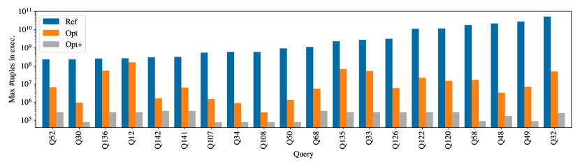
Figure 6. Comparison of the maximal number of materialised tuples in a table during query execution for 20 queries of STATS-CEB. Y-axis in logarithmic scale (base 10).

.

Throughout the paper, we have been motivated by the premise that standard logical optimisation rules for QEPs can avoid a significant amount of intermediate materialisation in aggregate queries. Moreover, with the addition of natural physical operators, we can avoid any such materialisation altogether. However, this raises the question of how much unnecessary materialisation actually occurs when using standard query planning methods.

To study this question directly, we compare the maximum number of tuples that occur in an intermediate table during query execution for the STATS-CEB queries. As with our reported times, the reported number of tuples is the average over 5 runs of the queries (we omit error bars as the variation between runs is mostly 0 and negligible in other cases). We note that these intermediate table sizes are naturally closely correlated to overall memory consumption, as well as communication cost in a distributed setting.

Figure 6 reports the peak number of materialised tuples during query execution for the 20 queries where standard Spark SQL materialises the most intermediate tuples. The data clearly shows that a significant improvement in the number of materialised tuples is often possible. In particular, we see that using standard Spark SQL query execution leads to clear intermediate blow-up of results. The largest relations in the dataset have in the order of $3\cdot 10^{5}$ tuples, an enormous difference to the observed sizes of intermediate results for Ref. The data shows that already by rewriting the logical QEPs according to Section 4, we regularly see an improvement of over 2 orders of magnitude.

However, as discussed above, this still requires some mild intermediate materialisation in between the intermediate aggregation steps. This becomes clear in comparison to the results for Opt⁺, which manages to consistently reduce the number of materialised tuples by at least 3 orders of magnitude on the reported queries in Figure 6. In fact, the reported numbers for Opt⁺ are always precisely the cardinality of the largest relation in the query, as the execution here never introduces any new tuples (cf. Section 5). That is, this number can also not be improved upon as long as the relations mentioned in the query are scanned at some point in query execution. Over the whole benchmark, we observe that the peak number of materialised tuples by Opt⁺ is at least 10 times lower than that of standard Spark SQL query execution in 118 out of the 146 queries. In all other cases, the peak number of materialised tuples by Ref and Opt⁺ is exactly the same, i.e., Ref is never better.

7. Conclusion

We have proposed the integration of optimisation techniques for certain kinds of aggregate queries into relational DBMSs with the goal of eliminating the materialisation of intermediate join results. To this end, we have targeted the recently presented class of 0MA-queries (Gottlob et al., 2023a, b) that allow for an evaluation based on semi-joins while completely avoiding the computation of joins. Moreover, we have shown how queries with COUNT and related aggregates (such as SUM, AVG, and MEDIAN) can be evaluated more efficiently by keeping track of multiplicities of tuples instead of materialising the tuples multiple times. We have implemented these optimisations into Spark SQL. By limiting the required changes of the query engine to the modification of subtrees of query execution plans and straightforward additional physical operators, we have illustrated that these optimisations are widely applicable to relational DBMSs. Our experimental evaluation confirms that these techniques can provide significant performance improvements and avoid large amounts of unnecessary materialisation in a variety of settings.

So far, we have applied our optimisation techniques only to 0MA queries and, more generally, to acyclic queries with guarded aggregation. In principle, the applicability of our methods can be immediately extended in two directions – dropping the acyclicity requirement and/or the guardedness requirement. Clearly, even if a query uses unguarded aggregation, we could create a guard by joining appropriate tables upfront. For instance, in the JOB benchmark, such an extension would allow us to cover almost all of the queries. Likewise, a cyclic query can always be transformed into an acyclic one via (generalised or fractional) hypertree decompositions (Gottlob et al., 2002b; Adler et al., 2007; Grohe and Marx, 2014). Again, the trick is to carry out some joins upfront so that the resulting relations form an acyclic query.

Of course, carrying out such joins upfront (to ensure guardedness and/or acyclicity) comes at a cost – both in terms of space and time. Our focus on guarded acyclic queries in this paper was motivated by no need for trade-offs, as our approach inherently never performs more work than traditional join plans. We leave it as an interesting open question for future research when extending our approach to cyclic and unguarded queries leads to a performance improvement compared with standard methods of query evaluation.

- (1)
- Aberger et al. (2017) Christopher R. Aberger, Andrew Lamb, Susan Tu, Andres Nötzli, Kunle Olukotun, and Christopher Ré. 2017. EmptyHeaded: A Relational Engine for Graph Processing. ACM Trans. Database Syst. 42, 4 (2017), 20:1–20:44. https://doi.org/10.1145/3129246
- Abiteboul et al. (1995) Serge Abiteboul, Richard Hull, and Victor Vianu. 1995. Foundations of Databases. Addison-Wesley. http://webdam.inria.fr/Alice/
- Adler et al. (2007) Isolde Adler, Georg Gottlob, and Martin Grohe. 2007. Hypertree width and related hypergraph invariants. Eur. J. Comb. 28, 8 (2007), 2167–2181. https://doi.org/10.1016/j.ejc.2007.04.013
- Afrati et al. (2017) Foto N. Afrati, Manas R. Joglekar, Christopher Ré, Semih Salihoglu, and Jeffrey D. Ullman. 2017. GYM: A Multiround Distributed Join Algorithm. In Proceedings ICDT (LIPIcs), Vol. 68. Schloss Dagstuhl - Leibniz-Zentrum für Informatik, 4:1–4:18. https://doi.org/10.4230/LIPIcs.ICDT.2017.4
- Armbrust et al. (2015) Michael Armbrust, Reynold S. Xin, Cheng Lian, Yin Huai, Davies Liu, Joseph K. Bradley, Xiangrui Meng, Tomer Kaftan, Michael J. Franklin, Ali Ghodsi, and Matei Zaharia. 2015. Spark SQL: Relational Data Processing in Spark. In Proceedings SIGMOD. ACM, 1383–1394. https://doi.org/10.1145/2723372.2742797
- Atserias et al. (2013) Albert Atserias, Martin Grohe, and Dániel Marx. 2013. Size Bounds and Query Plans for Relational Joins. SIAM J. Comput. 42, 4 (2013), 1737–1767. https://doi.org/10.1137/110859440
- Bagan et al. (2007) Guillaume Bagan, Arnaud Durand, and Etienne Grandjean. 2007. On Acyclic Conjunctive Queries and Constant Delay Enumeration. In Proceedings CSL (LNCS), Vol. 4646. Springer, 208–222. https://doi.org/10.1007/978-3-540-74915-8_18
- Bakibayev et al. (2013) Nurzhan Bakibayev, Tomás Kociský, Dan Olteanu, and Jakub Zavodny. 2013. Aggregation and Ordering in Factorised Databases. Proc. VLDB Endow. 6, 14 (2013), 1990–2001. https://doi.org/10.14778/2556549.2556579
- Baldacci and Golfarelli (2019) Lorenzo Baldacci and Matteo Golfarelli. 2019. A Cost Model for SPARK SQL. IEEE Trans. Knowl. Data Eng. 31, 5 (2019), 819–832. https://doi.org/10.1109/TKDE.2018.2850339
- Barceló et al. (2021) Pablo Barceló, Floris Geerts, Juan L. Reutter, and Maksimilian Ryschkov. 2021. Graph Neural Networks with Local Graph Parameters. In Proceedings NeurIPS. 25280–25293. https://proceedings.neurips.cc/paper/2021/hash/d4d8d1ac7e00e9105775a6b660dd3cbb-Abstract.html
- Chen and Dalmau (2012) Hubie Chen and Víctor Dalmau. 2012. Decomposing Quantified Conjunctive (or Disjunctive) Formulas. In Proceedings LICS. IEEE Computer Society, 205–214. https://doi.org/10.1109/LICS.2012.31
- Dai et al. (2023) Binyang Dai, Qichen Wang, and Ke Yi. 2023. SparkSQL+: Next-generation Query Planning over Spark. In Companion of the 2023 International Conference on Management of Data, SIGMOD/PODS 2023. ACM, 115–118. https://doi.org/10.1145/3555041.3589715
- Durand and Mengel (2015) Arnaud Durand and Stefan Mengel. 2015. Structural Tractability of Counting of Solutions to Conjunctive Queries. Theory Comput. Syst. 57, 4 (2015), 1202–1249. https://doi.org/10.1007/S00224-014-9543-Y
- Gottlob et al. (2023a) Georg Gottlob, Matthias Lanzinger, Davide Mario Longo, Cem Okulmus, Reinhard Pichler, and Alexander Selzer. 2023a. Reaching Back to Move Forward: Using Old Ideas to Achieve a New Level of Query Optimization (short paper). In Proceedings AMW (CEUR Workshop Proceedings), Vol. 3409. CEUR-WS.org. https://ceur-ws.org/Vol-3409/paper6.pdf
- Gottlob et al. (2023b) Georg Gottlob, Matthias Lanzinger, Davide Mario Longo, Cem Okulmus, Reinhard Pichler, and Alexander Selzer. 2023b. Structure-Guided Query Evaluation: Towards Bridging the Gap from Theory to Practice. CoRR abs/2303.02723 (2023). https://doi.org/10.48550/arXiv.2303.02723 arXiv:2303.02723
- Gottlob et al. (2001) Georg Gottlob, Nicola Leone, and Francesco Scarcello. 2001. J. ACM 48, 3 (2001), 431–498. https://doi.org/10.1145/382780.382783
- Gottlob et al. (2002a) Georg Gottlob, Nicola Leone, and Francesco Scarcello. 2002a. Hypertree Decompositions and Tractable Queries. J. Comput. Syst. Sci. 64, 3 (2002), 579–627. https://doi.org/10.1006/jcss.2001.1809
- Gottlob et al. (2002b) Georg Gottlob, Nicola Leone, and Francesco Scarcello. 2002b. Hypertree Decompositions and Tractable Queries. J. Comput. Syst. Sci. 64, 3 (2002), 579–627. https://doi.org/10.1006/JCSS.2001.1809
- Graham (1979) Marc H. Graham. 1979. On The Universal Relation. Technical Report. University of Toronto.
- Green et al. (2007) Todd J. Green, Gregory Karvounarakis, and Val Tannen. 2007. Provenance semirings. In Proceedings PODS. ACM, 31–40. https://doi.org/10.1145/1265530.1265535
- Grohe and Marx (2014) Martin Grohe and Dániel Marx. 2014. Constraint Solving via Fractional Edge Covers. ACM Trans. Algorithms 11, 1 (2014), 4:1–4:20.
- Han et al. (2021) Yuxing Han, Ziniu Wu, Peizhi Wu, Rong Zhu, Jingyi Yang, Liang Wei Tan, Kai Zeng, Gao Cong, Yanzhao Qin, Andreas Pfadler, Zhengping Qian, Jingren Zhou, Jiangneng Li, and Bin Cui. 2021. Cardinality Estimation in DBMS: A Comprehensive Benchmark Evaluation. Proc. VLDB Endow. 15, 4 (2021), 752–765. https://doi.org/10.14778/3503585.3503586
- Hu and Wang (2023) Xiao Hu and Qichen Wang. 2023. Computing the Difference of Conjunctive Queries Efficiently. Proc. ACM Manag. Data 1, 2 (2023), 153:1–153:26. https://doi.org/10.1145/3589298
- Hu and Miranker (2024) Zeyuan Hu and Daniel P. Miranker. 2024. TreeTracker Join: Turning the Tide When a Tuple Fails to Join. CoRR abs/2403.01631 (2024). arXiv:2403.01631 http://arxiv.org/abs/2403.01631
- Idris et al. (2017) Muhammad Idris, Martín Ugarte, and Stijn Vansummeren. 2017. The Dynamic Yannakakis Algorithm: Compact and Efficient Query Processing Under Updates. In Proceedings SIGMOD. ACM, 1259–1274. https://doi.org/10.1145/3035918.3064027
- Idris et al. (2020) Muhammad Idris, Martín Ugarte, Stijn Vansummeren, Hannes Voigt, and Wolfgang Lehner. 2020. General dynamic Yannakakis: conjunctive queries with theta joins under updates. VLDB J. 29, 2-3 (2020), 619–653. https://doi.org/10.1007/s00778-019-00590-9
- Ji et al. (2020) Xuechun Ji, Mao-Xian Zhao, Mingyu Zhai, and Qingxi Wu. 2020. Query Execution Optimization in Spark SQL. Sci. Program. 2020 (2020), 6364752:1–6364752:12. https://doi.org/10.1155/2020/6364752
- Jin et al. (2024) Emily Jin, Michael Bronstein, İsmail İlkan Ceylan, and Matthias Lanzinger. 2024. Homomorphism Counts for Graph Neural Networks: All About That Basis. CoRR abs/2402.08595 (2024). https://doi.org/10.48550/ARXIV.2402.08595 arXiv:2402.08595
- Joglekar et al. (2016) Manas R. Joglekar, Rohan Puttagunta, and Christopher Ré. 2016. AJAR: Aggregations and Joins over Annotated Relations. In Proceedings PODS. ACM, 91–106. https://doi.org/10.1145/2902251.2902293
- Khamis et al. (2016) Mahmoud Abo Khamis, Hung Q. Ngo, and Atri Rudra. 2016. FAQ: Questions Asked Frequently. In Proceedings PODS. ACM, 13–28. https://doi.org/10.1145/2902251.2902280
- Khayyat et al. (2015) Zuhair Khayyat, William Lucia, Meghna Singh, Mourad Ouzzani, Paolo Papotti, Jorge-Arnulfo Quiané-Ruiz, Nan Tang, and Panos Kalnis. 2015. Lightning Fast and Space Efficient Inequality Joins. Proc. VLDB Endow. 8, 13 (2015), 2074–2085. https://doi.org/10.14778/2831360.2831362
- Leis et al. (2015) Viktor Leis, Andrey Gubichev, Atanas Mirchev, Peter A. Boncz, Alfons Kemper, and Thomas Neumann. 2015. How Good Are Query Optimizers, Really? Proc. VLDB Endow. 9, 3 (2015), 204–215. https://doi.org/10.14778/2850583.2850594
- Leskovec and Krevl (2014) Jure Leskovec and Andrej Krevl. 2014. SNAP Datasets: Stanford Large Network Dataset Collection. http://snap.stanford.edu/data.
- Mancini et al. (2022) Riccardo Mancini, Srinivas Karthik, Bikash Chandra, Vasilis Mageirakos, and Anastasia Ailamaki. 2022. Efficient Massively Parallel Join Optimization for Large Queries. In Proceedings SIGMOD. ACM, 122–135. https://doi.org/10.1145/3514221.3517871
- Mhedhbi et al. (2021) Amine Mhedhbi, Matteo Lissandrini, Laurens Kuiper, Jack Waudby, and Gábor Szárnyas. 2021. LSQB: a large-scale subgraph query benchmark. In Proceedings GRADES. ACM, 8:1–8:11. https://doi.org/10.1145/3461837.3464516
- Misegiannis et al. (2022) Michail Georgoulakis Misegiannis, Vasiliki Kantere, and Laurent d’Orazio. 2022. Multi-objective query optimization in Spark SQL. In Proceedings IDEAS. ACM, 70–74. https://doi.org/10.1145/3548785.3548800
- Nguyen and Maehara (2020) Hoang Nguyen and Takanori Maehara. 2020. Graph Homomorphism Convolution. In Proceedings ICML (Proceedings of Machine Learning Research), Vol. 119. PMLR, 7306–7316. http://proceedings.mlr.press/v119/nguyen20c.html
- Olteanu and Závodný (2015) Dan Olteanu and Jakub Závodný. 2015. Size Bounds for Factorised Representations of Query Results. ACM Trans. Database Syst. 40, 1 (2015), 2:1–2:44. https://doi.org/10.1145/2656335
- Perelman and Ré (2015) Adam Perelman and Christopher Ré. 2015. DunceCap: Compiling Worst-Case Optimal Query Plans. In Proceedings SIGMOD. ACM, 2075–2076. https://doi.org/10.1145/2723372.2764945
- Pichler and Skritek (2013) Reinhard Pichler and Sebastian Skritek. 2013. Tractable counting of the answers to conjunctive queries. J. Comput. Syst. Sci. 79, 6 (2013), 984–1001. https://doi.org/10.1016/j.jcss.2013.01.012
- Seshadri et al. (1996) Praveen Seshadri, Hamid Pirahesh, and T. Y. Cliff Leung. 1996. Complex Query Decorrelation. In Proceedings ICDE. IEEE Computer Society, 450–458. https://doi.org/10.1109/ICDE.1996.492194
- Shen et al. (2023) Yu Shen, Xinyuyang Ren, Yupeng Lu, Huaijun Jiang, Huanyong Xu, Di Peng, Yang Li, Wentao Zhang, and Bin Cui. 2023. Rover: An Online Spark SQL Tuning Service via Generalized Transfer Learning. In Proceedings KDD. ACM, 4800–4812. https://doi.org/10.1145/3580305.3599953
- TPC-H ([n.d.]) TPC-H. [n.d.]. TPC-H Benchmark. https://www.tpc.org/tpch/.
- Tu and Ré (2015) Susan Tu and Christopher Ré. 2015. DunceCap: Query Plans Using Generalized Hypertree Decompositions. In Proceedings SIGMOD. ACM, 2077–2078. https://doi.org/10.1145/2723372.2764946
- Wang et al. (2023) Qichen Wang, Xiao Hu, Binyang Dai, and Ke Yi. 2023. Change Propagation Without Joins. CoRR abs/2301.04003 (2023). https://doi.org/10.48550/arXiv.2301.04003 arXiv:2301.04003
- Wang and Yi (2022) Qichen Wang and Ke Yi. 2022. Conjunctive Queries with Comparisons. In SIGMOD ’22: International Conference on Management of Data. ACM, 108–121. https://doi.org/10.1145/3514221.3517830
- Wang and Yi (2021) Yilei Wang and Ke Yi. 2021. Secure Yannakakis: Join-Aggregate Queries over Private Data. In SIGMOD ’21: International Conference on Management of Data. ACM, 1969–1981. https://doi.org/10.1145/3448016.3452808
- Yannakakis (1981) Mihalis Yannakakis. 1981. Algorithms for Acyclic Database Schemes. In Proceedings VLDB. VLDB, 82–94.
- Yu and Özsoyoğlu (1979) C. T. Yu and M. Z. Özsoyoğlu. 1979. An algorithm for tree-query membership of a distributed query. In The IEEE Computer Society’s Third International Computer Software and Applications Conference, COMPSAC 1979. 306–312.
- Zaharia et al. (2010) Matei Zaharia, Mosharaf Chowdhury, Michael J. Franklin, Scott Shenker, and Ion Stoica. 2010. Spark: Cluster Computing with Working Sets. In USENIX Workshop on Hot Topics in Cloud Computing. USENIX Association. https://www.usenix.org/conference/hotcloud-10/spark-cluster-computing-working-sets
- Zhai et al. (2019) Mingyu Zhai, Aibo Song, Jingyi Qiu, Xuechun Ji, and Qingxi Wu. 2019. Query optimization Approach with Shuffle Intermediate Cache Layer for Spark SQL. In Proceedings IPCCC. IEEE, 1–6. https://doi.org/10.1109/IPCCC47392.2019.8958719
- Zhang et al. (2020) Hao Zhang, Jeffrey Xu Yu, Yikai Zhang, Kangfei Zhao, and Hong Cheng. 2020. Distributed Subgraph Counting: A General Approach. Proc. VLDB Endow. 13, 11 (2020), 2493–2507. http://www.vldb.org/pvldb/vol13/p2493-zhang.pdf