Revising the Universality Hypothesis for Room-temperature Collisions

Abstract

Atoms constitute promising quantum sensors for a variety of scenarios including vacuum metrology. Key to this application is knowledge of the collision rate coefficient of the sensor atom with the particles being detected. Prior work demonstrated that, for room-temperature collisions, the total collision rate coefficient and the trap depth dependence of the sensor atom loss rate from shallow traps are both universal, independent of the interaction potential at short range. It was also shown that measurements of the energy transferred to the sensor atom by the collision can be used to estimate the total collision rate coefficient. However, discrepancies found when comparing the results of this and other methods of deducing the rate coefficient call into question its accuracy. Here the universality hypothesis is re-examined and an important correction is presented. We find that measurements of the post-collision recoil energy of sensor atoms held in shallow magnetic traps only provide information about the interaction potential at the very largest inter-atomic distances (e.g. the value of $C_{6}$ for a leading order term of $C_{6}/r^{6}$). As other non-negligible terms exist at medium and long ranges, the total collision rate coefficient, even if universal, can differ from that computed solely from the value of $C_{6}$. By incorporating these other long-range terms, the results align with full quantum mechanical scattering calculations, resolving the discrepancies and offering immediate implications for using atoms as a self-calibrating primary pressure standard.

I Introduction

Laser cooled atoms have been proposed [1, 2] and investigated [3, 4, 5, 6, 7, 8, 9, 10, 11, 12, 13, 14, 15, 16, 17, 18, 19] as a sensor for particles in vacuum. Specifically, the ambient gas number density, $\rho_{N}$, can be determined from measurements of the total collision rate of a stationary sensor atom with the ambient gas particles

$$\Gamma_{\rm{tot}}=\rho_{N}\left<\sigma_{\rm{tot}}\ v\right>(T)$$ (1)

where $\left<\sigma_{\rm{tot}}\ v\right>$ is referred to as the total collision rate coefficient and depends on the ambient gas temperature ($T$), $\sigma_{\rm{tot}}$ is the velocity-dependent cross section for the ambient gas and sensor particle collision, $v$ is the relative collision velocity, and the brackets denote an average over the Maxwell Boltzmann distribution of velocities for the ambient gas.

In practice, the sensor atoms are confined in a shallow trap, and the total collision rate is inferred from the observed trap loss rate,

$$\Gamma_{\rm{loss}}=\rho_{N}\left<\sigma_{\rm{loss}}\ v\right>(T,U),$$ (2)

where $\left<\sigma_{\rm{loss}}\ v\right>$ is the thermally-averaged loss rate coefficient. This coefficient depends on both the ambient gas temperature, $T$, and on the depth of the trap, $U$, confining the sensor atoms. In order for sensor atom loss to occur, a collision must transmit sufficient energy to the trapped atom that its energy exceeds the trap depth. In the limit $U\rightarrow 0$, the trap loss rate becomes the total collision rate, $\Gamma_{\rm{loss}}\rightarrow\Gamma_{\rm{tot}}$.

Deducing $\rho_{N}$ from Eqn. 1 or Eqn. 2 requires accurate knowledge of the rate coefficients. These coefficients can be inferred from measurements of the sensor atom loss rate at various trap depths, $\Gamma_{\rm{loss}}$, when exposed to a background gas of known density, $\rho_{N}$ [20, 21]. Unfortunately, this approach is limited to inert gas species compatible with the operation of existing orifice flow pressure standards (OFS). Alternatively, if the interaction potential between the sensor atom and the species of interest is known, the coefficient can be obtained from full quantum mechanical scattering calculations (FQMS) [22, 23, 24, 25, 26].

A third method is to use the so-called collision universality law to estimate the coefficient from measurements of the sensor atom collision recoil energy distribution [12, 27, 13, 14]. This approach was used to estimate the coefficients for ⁸⁷Rb sensor atoms with natural abundance H₂, He, N₂, Ar, CO₂, Kr, and Xe gases in Refs. [13, 14] and for natural abundance Rb gas collisions in Ref. [28]. Following that work, results from both theory calculations (FQMS) and orifice flow experiments (OFS) revealed differences in the values, at the level of a few percent, for the ⁸⁷Rb-X coefficients given X=N₂, Ar, Kr, and Xe gas particles as shown in Table 1. For X=H₂ gas, the FQMS result differed by more than 25% from the experimentally determined value. This motivated work that confirmed this larger discrepancy for ⁸⁷Rb-H₂ is due to the previously anticipated breakdown of the universality prescription for determining the coefficient between light collision partners [29].

The main goal of this work is to re-examine the original postulates of the collision universality law in an effort to understand the discrepancies observed in the $\left<\sigma_{\rm{tot}}\ v\right>$ values deduced for heavy collision partners using the universality prescription versus those found by FQMS reported in Ref. [26] and the OFS measurements reported in Refs. [20, 21].

The original universality hypothesis included three conjectures,

1. The total collision rate coefficient, $\left<\sigma_{\rm{tot}}\ v\right>$, is universal, determined solely by the long-range portion of the inter-species interaction potential. Namely, $\left<\sigma_{\rm{tot}}\ v\right>$ is independent of the details of the interaction potential at short range.

2. The trap loss rate coefficient is also universal, where $\rho_{N}\left<\sigma_{\rm{loss}}\ v\right>(U)$ is the rate of collisions that induce loss from a trap of depth $U$.

3. The variation of the loss rate coefficient with trap depth provides information about the total collision rate coefficient, $\left<\sigma_{\rm{tot}}\ v\right>$.

We show here, with data and computations, that first two postulates are sound but the third postulate needs revision. Specifically, we find that the sensor-atom collision-induced recoil energy distribution near zero energy, encoded in the loss rate versus trap depth from shallow traps ($U/k_{\rm{B}}<20$ mK), provides information about the leading order term, $-C_{6}/r^{6}$, of the interaction potential instead of the total collision rate coefficient. Although $\left<\sigma_{\rm{tot}}\ v\right>$ is dominated by the $C_{6}$ term and, for heavy collision partners, is insensitive to the shape of the interaction potential at short range, there are additional long range interactions, namely the $-C_{8}/r^{8}$ and $-C_{10}/r^{10}$ terms, that contribute to the total collision rate coefficient and make it distinct from that deduced using the universality prescription [12, 27, 13, 14]. By including these long-range interaction terms in a semi-classical analysis that provides a prediction of $\left<\sigma_{\rm{tot}}\ v\right>$ in the absence of any short range repulsive barrier, we find the prediction for heavy collision partners to be in excellent agreement with the full quantum scattering calculations reported in Ref. [26] at ambient temperature 21 C (294 K), differing by less than the stated uncertainties.

We believe these findings explain the observed discrepancies, reinforce the conjecture that room-temperature collisions are universal, insensitive to the short range interaction potential shape, and offer immediate implications for using atoms as a self-calibrating primary pressure standard.

System	$\left<\sigma_{\rm{tot}}\ v\right>$ ($10^{-15}$m3/s)
	QDU [14]	FQMS [26]	OFS [20]
87Rb-H2	5.12(15)	3.9(1)	—
87Rb-He	2.41(14)	2.37(3)	2.34(6)
87Rb-Ne	—	2.0(2)	2.21(5)
87Rb-N2	3.14(5)	3.45(6)	3.56(8)
87Rb-Ar	2.79(5)	3.035(7)	3.31(5)
87Rb-CO2	2.84(6)	—	—
87Rb-Kr	—	2.79(1)	2.79(4)
87Rb-Xe	2.75(4)	2.88(1)	2.95(7)

Table 1: Total collision rate coefficients, $\left<\sigma_{\rm{tot}}\ v\right>$, for ⁸⁷Rb when exposed to natural abundance versions of various species at a temperature of T=294 K as determined by the universal law of quantum diffractive collisions (QDU), FQMS calculations, and comparison with an orifice flow standard (OFS). All uncertainties are one-standard deviation $k=1$ (statistical) uncertainties.

This work is organized as follows: Section II reviews the theoretical framework for atom-atom elastic scattering and the original universality ansatz presented in Refs. [12, 13]. Section III reviews the physical origins of universality, illustrating how averaging the velocity-dependent collision cross section over the room-temperature Maxwell-Boltzmann distribution of incident speeds minimizes the influence of the potential shape at short range on the total collision rate coefficient, $\left<\sigma_{\rm{tot}}\ v\right>$. Section IV analyzes the effects of including the $C_{8}$ and $C_{10}$ long range interaction terms omitted in the original analysis. Using a purely long-range interaction potential of the form $V(r)=-C_{6}/r^{6}-C_{8}/r^{8}-C_{10}/r^{10}$, the total collision rate coefficients computed using a semi-classical (SC) description of the elastic scattering phase shifts (as an extension of the Jeffreys-Born (JB) ) approximation [30] are found to be in excellent agreement with FQMS computations using the interaction potentials published by Kłos and Tiesinga [26]. The agreement of the FQMS and SC values of $\left<\sigma_{\rm{tot}}\ v\right>$ reinforces the universality hypothesis. Finally, Section V uses FQMS computations for ⁷Li-X and ⁸⁷Rb-X (X = H₂, He, Ne, N₂, Ar, Kr, and Xe) collisions based on the interaction potentials published by Kłos and Tiesinga [26] to re-examine and redefine the relationship between $\left<\sigma_{\rm{loss}}\ v\right>$ and $\left<\sigma_{\rm{tot}}\ v\right>$.

II Review of the Universality Hypothesis

In this section, we review the quantum mechanical formulation of the total collision rate coefficient, $\left<\sigma_{\rm{tot}}\ v\right>$, and the trap loss rate coefficient, $\left<\sigma_{\rm{loss}}\ v\right>(U)$. We also present calculations of these coefficients using a Lennard-Jones interaction potential to illustrate the original universality ansatz presented in Refs. [12, 13].

We consider a collision between a stationary trapped atom of mass, $m_{t}$, and a background gas particle of mass $m_{b}$, whose speed is selected from the Maxwell-Boltzmann (MB) distribution of the particles at ambient temperature, $T$. The collision is analyzed in the center of mass (COM) frame where a reduced mass particle,

$$\mu=\frac{m_{t}m_{b}}{m_{t}+m_{b}}$$ (3)

scatters from the interaction potential, V(r), or from a potential energy surface, for lower symmetry collisions. In what follows, we will assume that the interaction potential is spherically symmetric. Although there exist anisotropic interactions from, for example, magnetic dipole-dipole interactions, these are exceedingly weak compared to the van der Waals interaction potential and are neglected in the following analysis.

For elastic scattering, the magnitude of the reduced mass particle’s momenta before ($\vec{p}=\hbar\vec{k}$) and after the collision ($\vec{p}^{\prime}=\hbar\vec{k}^{\prime}$) are equal. Only the direction of the momentum of the reduced mass particle is altered by the collision, rotating an amount $\theta$. Here $k=\mu v/\hbar$ is the magnitude of the wavevector describing the momentum of the incoming and outgoing reduced-mass particle, and $v$ is the relative speed of the colliding particles. From the kinematics of elastic collisions, one can deduce that the energy transferred to the (initially stationary) trapped particle in the laboratory frame is,

$$\Delta E_{t}=\frac{\mu^{2}v^{2}}{m_{t}}\left(1-\cos\theta\right).$$ (4)

In order to liberate a sensor atom from the trap, this energy must be greater than or equal to the trap depth, $U$ (for a stationary trapped atom). Rearranging Eq. 4 and setting $\Delta E_{t}=U$ one finds the corresponding minimum scattering angle required for trap loss is

$$\cos\theta_{\rm{min}}=1-\frac{m_{t}U}{\mu^{2}v^{2}},$$ (5)

which is explicitly dependent on the trap depth, $U$.

In the asymptotic region, far from the scattering center, the wave-function, in the COM frame, is the superposition of an incident plane wave and the scattered spherical wave, $\psi({\bf r})\xrightarrow[]{{\bf r}\rightarrow\infty}e^{ikz}+f(k,\theta)\frac{e^{ikr}}{r}$, where $f(k,\theta)$ quantifies the amplitude of scattering into the angle $\theta$ given an incident momentum $\hbar k$. The dependence of $f$ on $\phi$ is absent here since the scattering process does not change the azimuthal angle for a spherically symmetric potential. This scattering amplitude can be expressed as a sum of Legendre polynomials, $P_{L}\left(\cos\theta\right)$, weighted by the transition matrix elements $T_{L}(k)$, encoding the scattering amplitude into a particular “partial wave” with angular momentum $\hbar L$ as

$$f(k,\theta)=\frac{1}{k}\sum_{L}\left(2L+1\right)T_{L}(k)P_{L}\left(\cos\theta\right).$$ (6)

The total elastic collision cross-section for a scattering event with wavevector $k$ is then the sum of the scattering probability over all angles,

$$\sigma_{\rm{tot}}\left(k\right) = \int d\Omega\left|f(k,\theta)\right|^{2}$$ (7)

$$= \frac{1}{k^{2}}\int_{0}^{2\pi}d\phi\int_{0}^{\pi}\sin\theta d\theta\left[\sum_{L}\left(2L+1\right)T^{*}_{L}(k)P_{L}\left(\cos\theta\right)\right]$$

$$\ \ \ \ \ \ \ \ \ \ \ \ \ \ \ \ \ \ \ \ \ \ \ \times\left[\sum_{L^{\prime}}\left(2L^{\prime}+1\right)T_{L^{\prime}}(k)P_{L^{\prime}}\left(\cos\theta\right)\right].$$

The thermally averaged, total collision coefficient, $\left<\sigma_{\rm{tot}}\ v\right>$, is computed by averaging $\sigma_{\rm{tot}}(k)$ over the distribution of relative velocities in the center-of-mass frame. To compute this average, we approximate the relative speed distribution of the collision partners using the lab frame Maxwell-Boltzmann (MB) speed distribution, $d(v)$, of the background gas particles at room temperature. This approach is exact in the limit that the trapped sensor particle is stationary, and, as shown in Ref. [31], this approximation is justified here because the energy of the sensor atoms in the trap is on the order of $10^{6}$ times smaller than the energy of the background gas particles.

$$\left<\sigma_{\rm{tot}}\ v\right> = \int_{0}^{\infty}d(v)dv\left(2\pi\cdot v\int_{0}^{\pi}\sin\theta d\theta\left|f\left(k,\theta\right)\right|^{2}\right)$$ (8)

$$= \left<2\pi\cdot v\int_{0}^{\pi}\sin\theta d\theta\left|f\left(k,\theta\right)\right|^{2}\right>$$

where the speed distribution is

$$d(v)dv = 4\pi\left(\dfrac{m_{b}}{2\pi k_{\rm{B}}T}\right)^{3/2}v^{2}e^{-m_{b}v^{2}/2k_{\rm{B}}T}dv$$ (9)

$$= \frac{4}{\sqrt{\pi}}\left(\frac{v}{v_{p}}\right)^{2}e^{-\left(\frac{v}{v_{p}}\right)^{2}}\frac{dv}{v_{p}}.$$

Here $v_{p}=\sqrt{2k_{B}T/m_{b}}$ is the peak speed of the distribution.

Trap loss only occurs for $\theta\in[\theta_{\rm{min}},\pi]$, leading to the thermally averaged trap loss rate coefficient,

$$\left<\sigma_{\rm{loss}}\ v\right>=\left<2\pi\cdot v\int_{\theta_{\rm{min}}}^{\pi}\sin\theta d\theta\left|f\left(k,\theta\right)\right|^{2}\right>.$$ (10)

Here $\theta_{\rm{min}}$ is given by Eq. 5 and is dependent on both the relative collision velocity, $v$, and the sensor atom trap depth, $U$. Without loss of generality, one can re-write Eq. 10 as,

$$\left<\sigma_{\rm{loss}}\ v\right> = \left<2\pi\cdot v\int_{0}^{\pi}\sin\theta d\theta\left|f\left(k,\theta\right)\right|^{2}\right>$$ (11)

$$-\left<2\pi\cdot v\int_{0}^{\theta_{\rm{min}}}\sin\theta d\theta\left|f\left(k,\theta\right)\right|^{2}\right>$$

$$= \left<\sigma_{\rm{tot}}\ v\right>-\left<2\pi\cdot v\int_{0}^{\theta_{\rm{min}}}\sin\theta d\theta\left|f\left(k,\theta\right)\right|^{2}\right>$$

$$= \left<\sigma_{\rm{tot}}\ v\right>\left[1-\frac{\left<2\pi\cdot v\int_{0}^{\theta_{\rm{min}}}\sin\theta d\theta\left|f\left(k,\theta\right)\right|^{2}\right>}{\left<\sigma_{\rm{tot}}\ v\right>}\right]$$

$$= \left<\sigma_{\rm{tot}}\ v\right>\left[1-p(U)\right].$$

The quantity,

$$p(U)=\frac{\left<2\pi\cdot v\int_{0}^{\theta_{\rm{min}}(U)}\sin\theta d\theta\left|f\left(k,\theta\right)\right|^{2}\right>}{\left<\sigma_{\rm{tot}}\ v\right>}$$ (12)

is the the cumulative probability that a collision imparts an energy $\Delta E_{t}\leq U$ to the sensor atom.

Evidence that this cumulative probability distribution is a universal function, insensitive to the interaction potential at short range, was reported in Refs. [12, 13, 14]. Specifically, it was asserted that $p(U)=p_{\mathrm{QDU}}(U/U_{\rm{d}})$ for any collision pair where $p_{\mathrm{QDU}}(x)$ is a universal function and $U_{\rm{d}}$ is the so-called quantum diffractive energy:

$$U_{\rm{d}}=\frac{4\pi\hbar^{2}}{m_{t}\bar{\sigma}},$$ (13)

where $m_{t}$ is the mass of the trapped sensor atom, $\bar{\sigma}\leavevmode\nobreak\ =\leavevmode\nobreak\ \left<\sigma_{\rm{tot}}\ v\right>/v_{\rm{p}}$ is the effective collision cross-section, and $v_{\rm{p}}$ is the peak speed of the MB distribution of the background species impinging on the sensor atom. This is the natural energy scale associated with a collision-induced localization of the sensor atom to a region of size $\sqrt{\bar{\sigma}}\$ [12]. As discussed in Ref. [32], the term “diffractive collisions” comes from the notion that for hard sphere quantum scattering, where $R$ is the range of the interaction potential, half of the total cross section ($\sigma\simeq 2\pi R^{2}$) is accounted for by “classical” scattering with a geometric cross section of $\pi R^{2}$ and an additional $\pi R^{2}$ is due to diffraction [30].

In the original investigation into universality [12, 13], FQMS computations were carried out with a Lennard-Jones (LJ) model for the interaction potential,

$$V(r) = \frac{C_{12}}{r^{12}}-\frac{C_{6}}{r^{6}}$$ (14)

where $C_{12}=C_{6}^{2}/(4D_{e})$ and $D_{e}$ is the depth of the interaction potential. For illustration purposes, we show here the results of FQMS calculations for the total collision rate and the trap depth dependent loss rate coefficients at an ambient temperature of 294 K using the LJ interaction model. Figure 1(a) shows the ratio $\left<\sigma_{\rm{loss}}\ v\right>(U)/\left<\sigma_{\rm{tot}}\ v\right>$ versus trap depth for ⁸⁷Rb-Ar, ⁸⁷Rb-Kr, and ⁸⁷Rb-Xe collision partners, using the $C_{6}$ and $D_{e}$ values from [26]. This ratio, per Eq. 11, is equal to $1-p(U)$, and the separation of the individual curves in Fig. 1(a) indicates that $p(U)$ is different for each collision pair. However, when the energy axis is re-scaled by the corresponding value of $U_{\rm{d}}$ in each case (defined in Eqn. 13) the curves, shown in Fig. 1(b) at low trap depths, collapse to the same function.

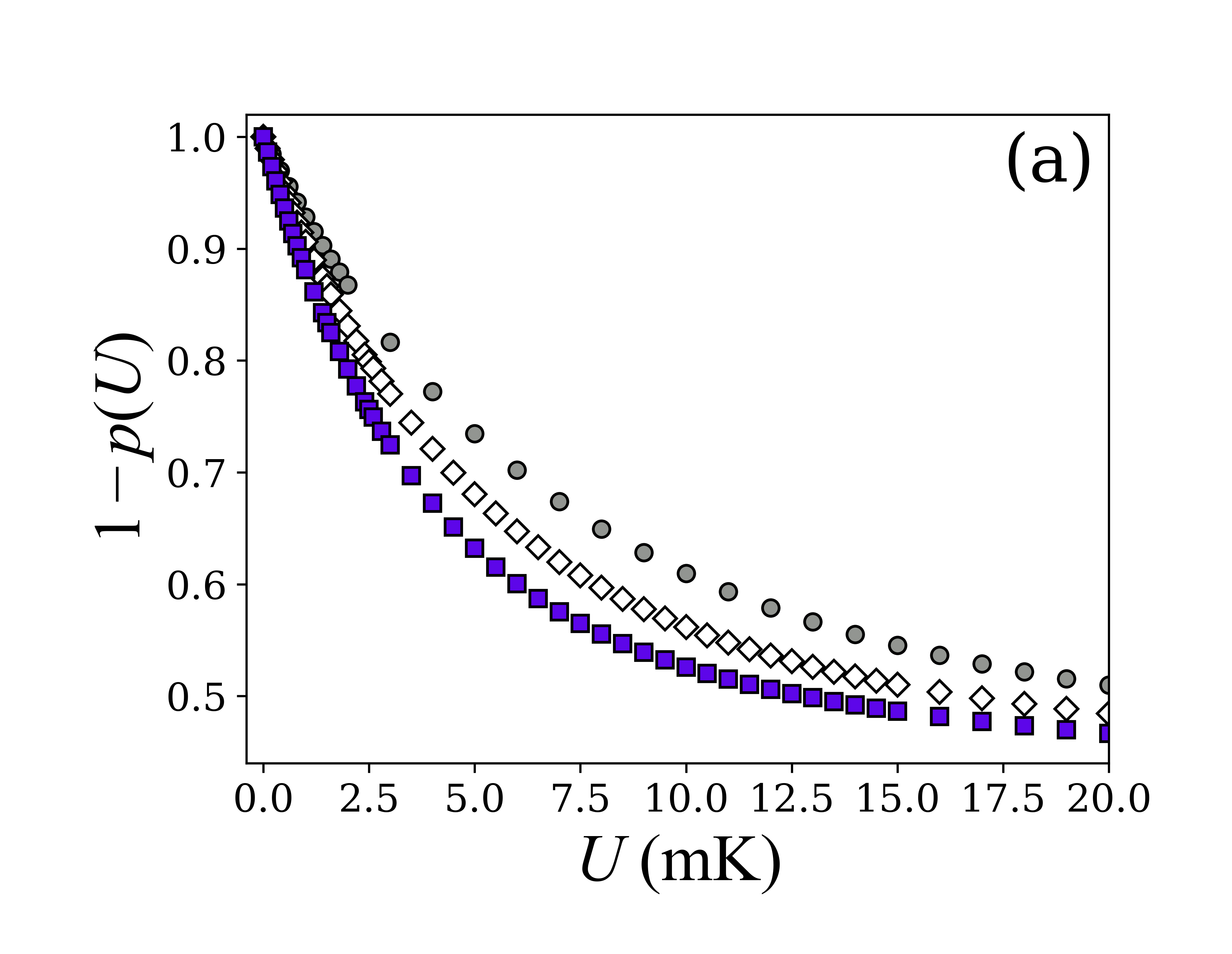
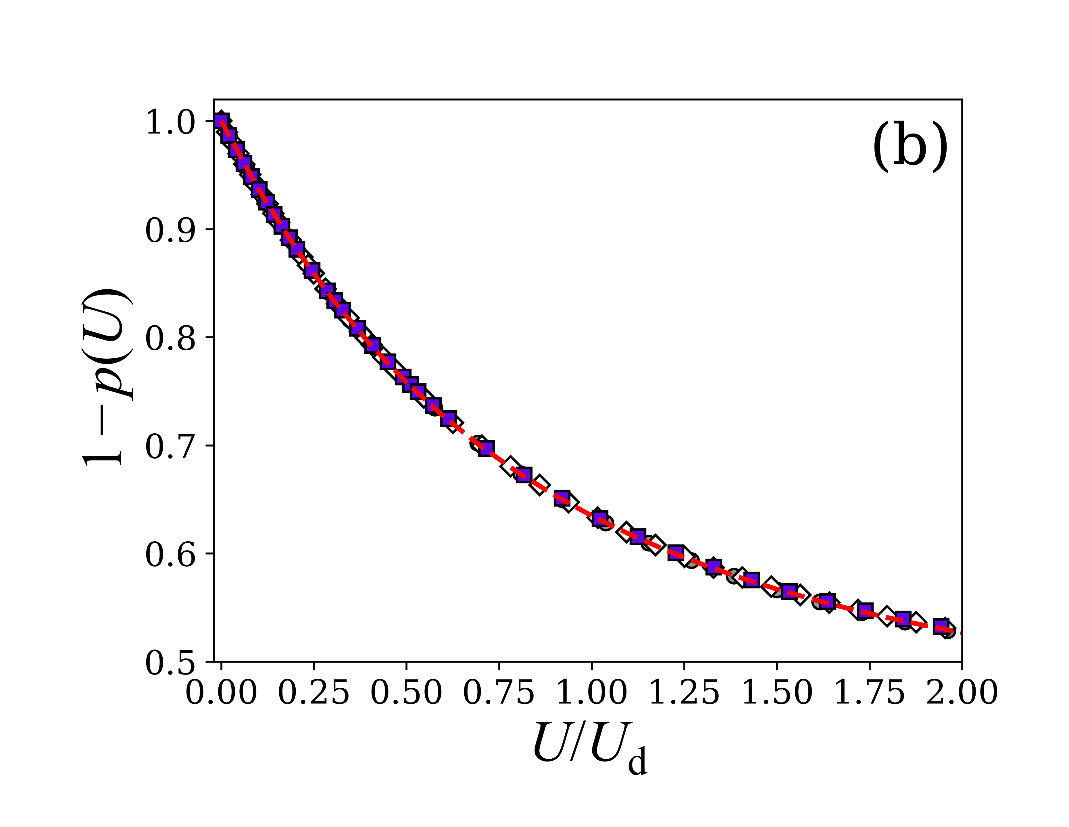
Figure 1: The ratio of the trap loss rate coefficient to the total collision rate coefficient, $\left<\sigma_{\rm{loss}}\ v\right>/\left<\sigma_{\rm{tot}}\ v\right>=1-p(U)$, computed using FQMS calculations for a Lennard Jones potential with the $C_{6}$ and $D_{e}$ values from Ref. [26] at T = 294 K. The results for ⁸⁷Rb-Ar (grey circles), ⁸⁷Rb-Kr (white diamonds), and ⁸⁷Rb-Xe (violet squares) are plotted (a) versus trap depth, $U$, and (b) versus $U/U_{\rm{d}}$. The red dashed curve is the polynomial approximation to the universal function, $1-p_{\rm{QDU}}(U/U_{\rm{d}})$, defined in Eq. 15 and Table 2.

This observation motivated the authors of Ref. [12] to assert that the $p(U)$ functions are given by

$$p(U)=p_{\mathrm{QDU}}\left(\frac{U}{U_{\rm{d}}}\right)\simeq\sum_{j}\beta_{j}\left(\frac{U}{U_{\rm{d}}}\right)^{j}.$$ (15)

where the universal function, $p_{\mathrm{QDU}}$, is approximated by a sixth order polynomial over the range $U/U_{\rm{d}}\leq 2$. The coefficients, $\beta_{j}$, listed in Table 2, are common to all universal collision partners [12].

Coefficient	—Value
$\beta_{1}$	0.673(7)
$\beta_{2}$	-0.477(3)
$\beta_{3}$	0.228(6)
$\beta_{4}$	-0.0703(42)
$\beta_{5}$	0.0123(14)
$\beta_{6}$	-0.0009(2)

Table 2: The coefficients, $\beta_{j}$, of the polynomial approximation to the universal function, $p_{\mathrm{QDU}}$, in Eqn. 15 as reported in Refs. [12, 13]

This formulation provides an empirical method for determining $\left<\sigma_{\rm{tot}}\ v\right>$ by fitting the normalized loss rate measurements, $\Gamma_{\rm{loss}}(U)/\Gamma_{\rm{loss}}(U=0)$, at different trap depths to the universal expression, Eq. 15, extracting $U_{\rm{d}}$ and then deducing $\left<\sigma_{\rm{tot}}\ v\right>$ using Eq. 13. This procedure was used in Refs. [12, 13, 14] to obtain the total collision rate coefficients from the variation of the loss rate with trap depth. These results are compared, in Table 1, to those obtained from FQMS and from loss rate measurements at known gas densities using an orifice flow standard (OFS). The observed discrepancies call into question the accuracy of this empirical method and are the motivation of the present work.

The LJ potential used here and in prior work on this topic does not provide a physically accurate model of the core repulsion between the colliding partners. In addition, it ignores the $C_{8}$ and $C_{10}$ long-range terms. The former inadequacy is somewhat irrelevant for universal collision partners; however, the result of omitting the long-range terms is that the total collision rate coefficient $\left<\sigma_{\rm{tot}}\ v\right>$ computed using the LJ potential for a universal collision pair is not the true rate coefficient, which is influenced by all long range terms. Instead, quantum scattering calculations with the LJ potential yield a rate coefficient equal to that obtained for a purely $C_{6}$ potential of the form $V(r)=-C_{6}/r^{6}$.

Because, as we will show, fitting the normalized loss rate variation with trap depth for a universal collision pair provides the $U_{\rm{d},6}$ value, corresponding to $\left<\sigma_{\rm{tot}}v\right>_{\rm{C6}}$, the fit does furnish the same total collision rate coefficient obtained by FQMS calculations for LJ potential. Thus, the authors of Ref. [12] concluded, incorrectly, that the empirical $U_{\rm{d}}$ values obtained by fitting the normalized loss rate to the universality law are equal to the total collision rate coefficient.

III The basis and breakdown of Collision Universality

It is well known from experiments with molecular beams that $\sigma_{\rm{tot}}(k)$ (Eq. 7) exhibits undulatory variations as a function of the relative-velocity about a trend dictated by the long range part of the interaction potential [33, 34, 30]. These undulations arise from the core-induced, low angular momentum (low $L$) partial waves scattered in the forward direction (referred to as “glory scattering”) which interfere with the high angular momentum (high $L$) partial wave scattering at small angles associated with the long range portion of the interaction potential. The iconic halo around an observer’s shadow created by optical glory scattering in water droplets of a cloud corresponds to backward ($\theta=\pi$) glory scattering (also observed in molecular beam experiments [35]). Whereas forward glory scattering at $\theta=0$, recently observed in molecular beam experiments [36], is responsible for creating the undulations in the total cross section. Changes of the shape of the interaction potential at short range change the number, the amplitude, and the locations of the undulatory variations. Above a critical velocity, referred to here as $v_{\rm{G}}$, the glory oscillations cease and $\sigma_{\rm{tot}}(k)$ transitions to following the monotonic trend set by the short range interaction potential.

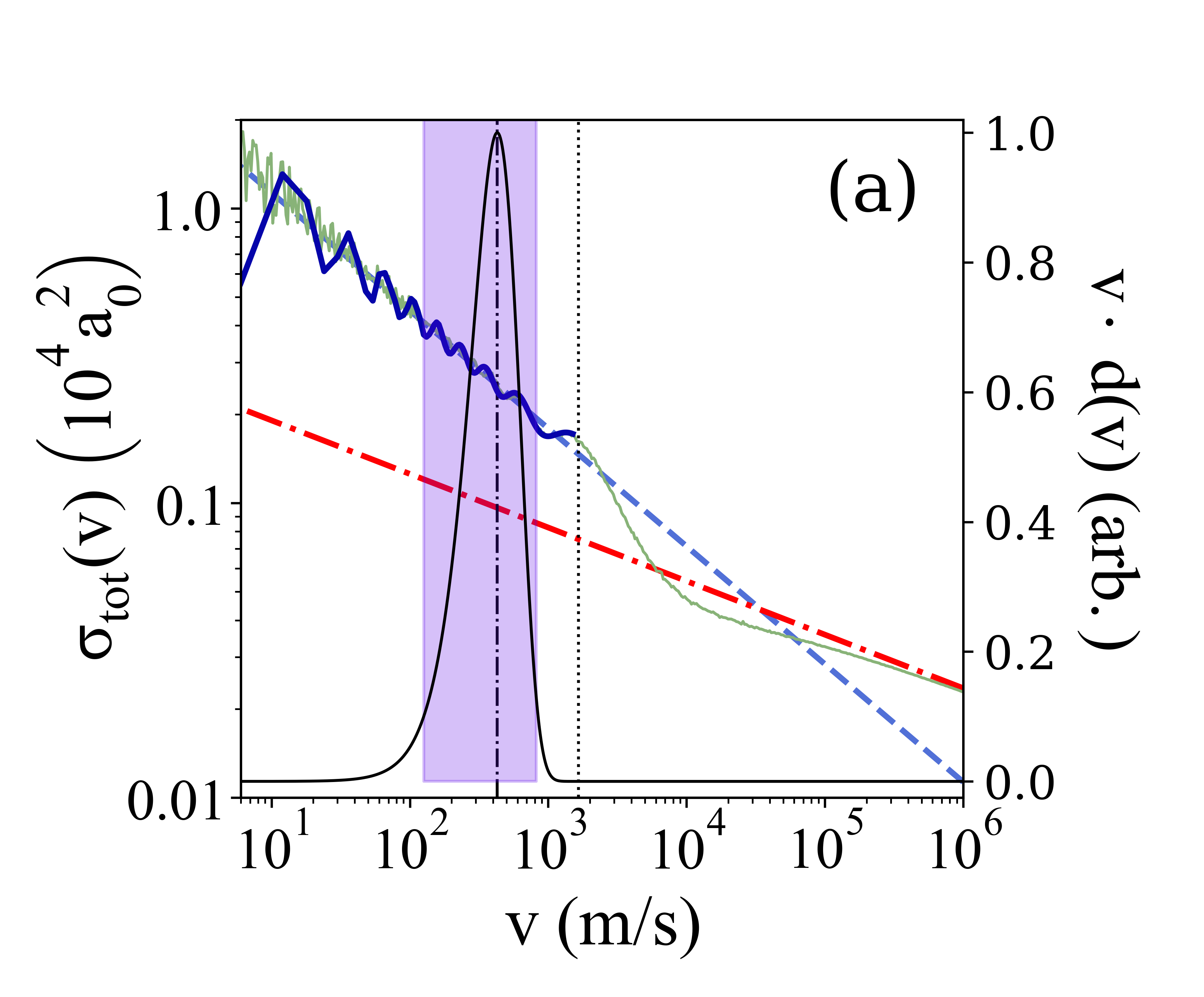
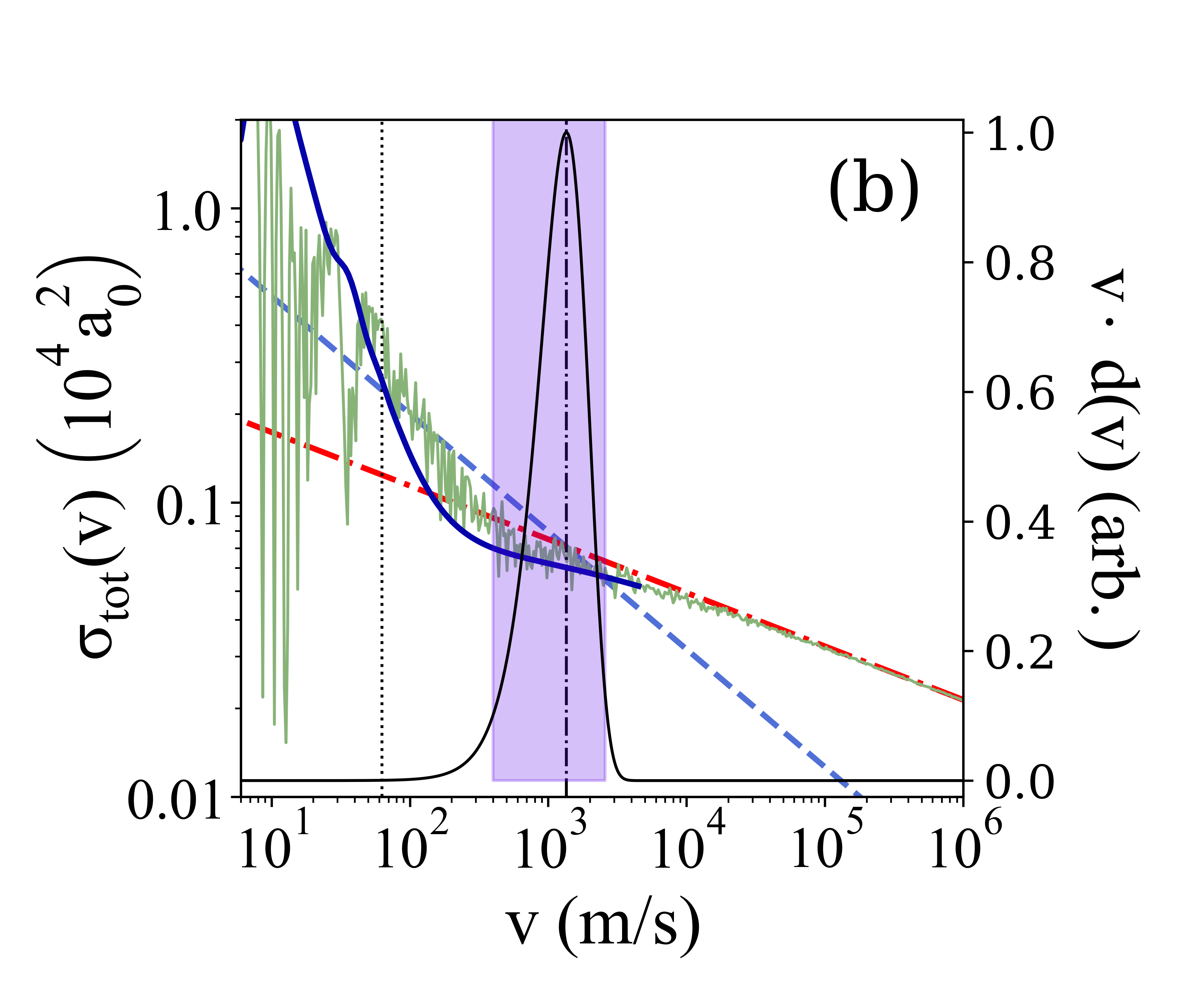
Figure 2: Comparison of the $\sigma_{\rm{tot}}$ versus $v$ for (a) ⁸⁷Rb-Ar and (b) ⁸⁷Rb-He based on Lennard-Jones (LJ) interaction potentials at T = 294K. The blue dashed traces are the predictions for a pure long-range $C_{6}$ potential, Eq. 18, and the red dot-dashed traces are the the pure short-range $C_{12}$ potential predictions, Eq. 20. The thin green traces show $\sigma_{\rm{tot}}(v)$ computed using the LJ potential with the Jeffreys-Born (JB) approximation for the elastic scattering phase shifts, Eq. 17 and 19. Note how the green traces follow the pure long range ($C_{6}$) prediction, then transition towards the pure short-range ($C_{12}$) prediction for large relative collision speeds, $v>v^{\rm{max}}_{C6}$. The FQMS LJ computations are shown as the thick blue traces. The characteristic glory oscillations around the purely $C_{6}$ predictions are evident for the ⁸⁷Rb-Ar results, while these are missing for the low mass collision partner, ⁸⁷Rb-He, because the number of bound states is exceedingly low for this latter case (see the appendix). For both figures, the position of the final (largest speed) glory undulation maxmimum is indicated by the vertical dotted black line at $v^{\rm{max}}_{C6}$. Finally, the velocity-weighted MB distributions, $v\cdot d(v)$ are shown. The shaded region indicates the range over which $v\cdot d(v)\geq 0.1$. This provides a visual reference for the range of $v$ which contribute the most to the total collision coefficients, $\left<\sigma_{\rm{tot}}\ v\right>$.

To illustrate this behavior Fig. 2 shows plots of $\sigma_{\rm{tot}}(v\leavevmode\nobreak\ =\leavevmode\nobreak\ \hbar\leavevmode\nobreak\ k/\mu)$ versus $v$, for (i) a purely long range $C_{6}$ potential, of the form $V(r)=-C_{6}/r^{6}$ (blue dashed traces), (ii) a purely repulsive $C_{12}$ potential, $V(r)=C_{12}/r^{12}$ (red dot-dashed traces), and (iii) the combination of these two terms to form the Lennard-Jones (LJ) potential where we compute $\sigma_{\rm{tot}}(v)$ using both an approximate solution (solid green trace) and the results of a FQMS calculation (solid blue trace). (Note the FQMS computations were performed over a more limited range of relative collision speeds owing to the increasingly longer computation duration required for convergence of the results at larger $v$ values.)

We determine the scattering cross section by computing the scattering amplitude, Eq. 6, where the physics of the interaction is contained in the transition matrix elements

$$T_{L}(k)=e^{i\eta_{\rm{L}}(k)}\sin\left(\eta_{\rm{L}}(k)\right).$$ (16)

The $\eta_{\rm{L}}(k)$ are the momentum-dependent phase shifts for each partial wave. For a purely long range $C_{6}$ potential, these phase shifts can be estimated using the Jeffreys-Born (JB) approximation [30], valid for large $L$,

$$\eta_{\rm{L}}(k,C_{6})=\frac{3\pi}{16}\left(\frac{\mu C_{6}}{\hbar^{2}}\right)\frac{k^{4}}{\ell^{5}},$$ (17)

where $\ell=L+1/2$. The inclusion of the $1/2$ in this definition of $\eta_{\rm{L}}(k)$ insures that the value remains finite for $L=0$. In the large $L$ limit the $1/2$ is irrelevant and can be neglected.

Using this in Eq. 7 and approximating the sum over $L$ as an integral over $dL$, we obtain

$$\sigma_{\rm{tot}}^{\rm{C6}}(v)\approx 8.0828\left(\frac{C_{6}}{\hbar v}\right)^{\frac{2}{5}}$$ (18)

Here the relative speed of the collision, $v=\hbar k/\mu$, is used in place of $k$, and this expression is plotted as the blue dashed traces in Fig. 2(a) and (b). An analogous JB approximation can be found for the phase shifts corresponding to a purely $C_{12}/r^{12}$ repulsive potential:

$$\eta_{\rm{L}}(k,C_{12})=-\frac{63\pi}{512}\left(\frac{\mu C_{12}}{\hbar^{2}}\right)\frac{k^{10}}{\ell^{11}}=-\frac{63\pi}{512}\left(\frac{\mu C_{6}^{2}}{4D_{e}\hbar^{2}}\right)\frac{k^{10}}{\ell^{11}}.$$ (19)

This phase shift yields the velocity dependent cross section,

$$\sigma_{\rm{tot}}^{C12}(v) \approx 6.583934\left(\frac{C_{12}}{\hbar v}\right)^{\frac{2}{11}}$$ (20)

corresponding to the red dot-dashed traces on Fig. 2(a) and (b).

The phase shifts for a Lennard-Jones potential can be approximated as the sum of these,

$$\eta_{\rm{L}}(k,\mathrm{LJ})=\eta_{\rm{L}}(k,C_{12})+\eta_{\rm{L}}(k,C_{6}).$$ (21)

The resulting velocity dependent LJ cross section approximation is shown as the thin green traces on Fig. 2(a) and (b). Also shown in Fig. 2 are the exact $\sigma_{\rm{tot}}(v)$ found by FQMS calculations (solid blue traces). The agreement is good at large velocities where the JB approximation is valid. (Note the range of $v$ used in the FQMS computation was limited to $0\leq v\leq 4\cdot v_{\rm{p}}$ due to the rapidly increased computation time needed to achieve convergence for larger $v$ values.)

As discussed above, the inclusion of a core repulsion in the interaction potential, here a $C_{12}/r^{12}$ term in the LJ potential, modifies the phase shifts to induce an oscillatory behavior in the $\sigma_{\rm{tot}}(v)$ about the purely long range potential prediction, Eqn. 18, at low relative collision speeds. At large relative collision speeds, the behavior of $\sigma_{\rm{tot}}(v)$ transitions to follow the prediction based on the purely short range part of the potential, Eqn. 20. The transition velocity, defined here as the location of the final, high $v$, glory oscillation maximum, can be found analytically for the LJ potential using the JB approximation. (See the appendix.) It is

$$v^{\rm{max}}_{C6} = 0.120496\cdot v_{\rm{G}}$$ (22)

where

$$v_{\rm{G}} = \frac{4D_{e}R_{0}}{\hbar}$$ (23)

and $R_{0}=[C_{6}/(4D_{e})]^{1/6}$ is the inter-species separation at which the LJ potential is zero (i.e. $V_{\rm{LJ}}(R_{0})=0$). The $v^{\rm{max}}_{C6}$ for the LJ potentials are indicated by the black vertical dotted lines in Fig. 2(a) and (b). In short, one may define the long-range ($C_{6}$) dominated domain as $v\leq v^{\rm{max}}_{C6}$.

Also shown in Fig. 2 is the velocity-weighted MB distribution, $v\cdot d(v)$, (thin black solid trace) for a room-temperature ($T=294$ K) gas of Ar in Fig. 2(a) and for He in Fig. 2(b). The speed corresponding to the maximum of this normalized distribution, $v_{vdv}^{\rm{max}}=\sqrt{3/2}v_{\rm{p}}$, is shown as the black vertical dash-dotted line on each figure. The shaded region overlaid on the normalized distributions indicates the range of speeds for which $v\cdot d(v)\geq 0.1$ (i.e. $0.36v_{\rm{p}}\leq v\leq 2.42v_{\rm{p}}$) as an aid to visualizing the weight and region over which the average $\left<\sigma_{\rm{tot}}\ v\right>$ is computed. The room temperature (T = 294 K) distribution, $v\cdot d(v)$, for ⁸⁷Rb-Ar collisions reaches a maximum at a value well below $v^{\rm{max}}_{C6}$ ($v_{vdv}^{\rm{max}}<v^{\rm{max}}_{C6}$) and spans several glory oscillations minimizing their influence on the velocity averaged quantities, $\left<\sigma_{\rm{tot}}\ v\right>$ and $\left<\sigma_{\rm{loss}}\ v\right>$. This makes these velocity averaged quantities insensitive to the details of the glory undulations and, thus, insensitive to the short range interaction potential shape [12]. By contrast, one observes that the velocity weighted distribution for ⁸⁷Rb-He encompasses the domain where the underlying character of the $\sigma_{\rm{tot}}(v)$ transitions from a purely long-range ($C_{6}$) to a purely short-range ($C_{12}$) dominated behavior occurring where $v_{vdv}^{\rm{max}}>v^{\rm{max}}_{C6}$. Thus, the ⁸⁷Rb-He collisions are not universal.

Two properties of the glory oscillations relevant to universality from velocity averaging are [33, 34, 30, 37] (also see Appendix A),

1. The amplitude of the glory oscillations decreases as the reduced mass of the colliding partners increases.

2. The number of oscillations per unit speed increases with increased reduced mass of the collision partners.

Thus, for heavier collision partners, one observes low amplitude, high frequency (in speed or wavenumber) glory oscillations leading to an even more complete suppression of the short range influence.

The velocity averaging erasure of the glory scattering effects is the origin of the total collision rate universality for heavy collision partners. The result is that the $\left<\sigma_{\rm{tot}}\ v\right>$ value computed from a given interaction potential is very close to that obtained from a different potential with the same long range behavior but a radically different short range repulsive barrier [12]. This feature is particularly significant to vacuum metrology because it implies that errors or uncertainties in the short-range part of the interaction potential do not propagate to the total collision rate coefficient and thus to the density or pressure inferred from a measurement.

III.1 Universality breakdown

Key to universality is the width and position of the relative velocity distribution, $v\cdot d(v)$, compared to the period and the amplitude of the glory undulations associated with the collisions. A hard limit for the breakdown of the universality hypothesis can be defined as when $v_{vdv}^{\rm{max}}>v^{\rm{max}}_{C6}$. That is, when the velocity averaging region lies outside the long-range $C_{6}$ characteristic regime (defined by $v<v^{\rm{max}}_{C6}$) then the short-range character of the collision process becomes dominant. This can occur either because the background gas temperature is too high or because the background species is very light, so the total collision and loss rate coefficients will not be universal, but will depend on the interaction potential at short range. As seen in Fig. 2, significant weight for the ⁸⁷Rb-He velocity distribution occurs above $v^{\rm{max}}_{C6}$ (= 62 m/s) and makes the value of $\left<\sigma_{\rm{tot}}\ v\right>$ sensitive to the short-range interaction potential shape.

A second limit for the breakdown of universality occurs if the distribution of relative collision velocities is too narrow compared to the period of the glory undulations, even if $v_{vdv}^{\rm{max}}<v^{\rm{max}}_{C6}$. This can happen in a molecular beam experiment or when the background species is extremely cold, rendering the range of velocity averaging small compared to the period of the glory undulations.

To substantiate this discussion, we compare $\left<\sigma_{\rm{tot}}\ v\right>$ values at $T=294$ K computed by FQMS calculations for a LJ potential with the approximate prediction for a pure long-range $C_{6}$ potential,

$$\left<\sigma_{\rm{tot}}v\right>_{\rm{C6}}\approx 8.49464\left(\frac{C_{6}}{\hbar v_{\rm{p}}}\right)^{\frac{2}{5}}v_{p}$$ (24)

where $v_{\rm{p}}$ is the peak of the MB speed distribution. (See Table 3.) Although the effects of the short range potential are completely absent in the latter case, the predictions are in close agreement with the FQMS values, and the differences are less than 0.5% for the heavy collision partners. However, for collisions with lighter background particles the results are different by up to $\simeq\leavevmode\nobreak\ 20$%, indicating that the $\left<\sigma_{\rm{tot}}\ v\right>$ values are significantly impacted by the core repulsion.

In addition, Table 3 contains the values of $v_{vdv}^{\rm{max}}$ and $v^{\rm{max}}_{C6}$ for each of these collision partners. As per the discussion, the non-universal species listed here (⁸⁷Rb-He and ⁸⁷Rb-Ne) share the characteristic that $v_{vdv}^{\rm{max}}>v^{\rm{max}}_{C6}$, indicating that the velocity averaging occurs outside the $C_{6}$ - dominated collision region.

	($10^{-15}$m3/s)		(m/s)
Collision Pair	$\left<\sigma_{\rm{tot}}v\right>_{\rm{C6}}$	$\left<\sigma_{\rm{tot}}\ v\right>_{\rm{LJ}}$	$v_{vdv}^{\rm{max}}$	$v^{\rm{max}}_{C6}$
87Rb-He	2.49	2.10	1354	62
87Rb-Ne	2.01	1.72	603	281
87Rb-Ar	2.81	2.82	428	1638
87Rb-Kr	2.63	2.64	296	2785
87Rb-Xe	2.75	2.76	236	4243

Table 3: Comparison of $\left<\sigma_{\rm{tot}}\ v\right>$ values given an interaction potential with and without its short range repulsive barrier for a variety of collision partners. The $\left<\sigma_{\rm{tot}}\ v\right>_{\rm{LJ}}$ are from FQMS computations using a Lennard-Jones potential, while the $\left<\sigma_{\rm{tot}}v\right>_{\rm{C6}}$ are the JB approximation for a purely $C_{6}$ potential, Eq. 24. Note the close agreement between these two values for the heavier collision partners, ⁸⁷Rb-Ar, ⁸⁷Rb-Kr, and ⁸⁷Rb-Xe. The final two columns indicate the values of $v_{vdv}^{\rm{max}}$ and $v^{\rm{max}}_{C6}$ for each species. As expected, the universal species share the characteristic that $v_{vdv}^{\rm{max}}<v^{\rm{max}}_{C6}$. For all of the entries the ambient temperature was chosen as 294K for the MB averaging, and the $C_{6}$ and $D_{e}$ parameters are taken from [26].

IV Universality Revisited

In the previous sections, the universality hypothesis was illustrated using the LJ potential. In this section, we examine the validity of the universality hypothesis using more realistic models of the interaction potentials taken from Medvedev et al [38] and Kłos and Tiesinga [26]. For this purpose, we develop a more accurate semi-classical model (SC) including the other long-range van der Waals interactions, $-C_{8}/r^{8}$ and $-C_{10}/r^{10}$, that were omitted in prior work and in the preceding analysis.

IV.1 Including $C_{8}$ and $C_{10}$ long range terms.

The other long-range van der Waals interactions, $-C_{8}/r^{8}$ and $-C_{10}/r^{10}$, that were omitted in prior work and in the preceding analysis add to the collision phase shifts, $\eta_{L}(k)$, and, increase the $\sigma_{\rm{tot}}(v)$ and $\left<\sigma_{\rm{tot}}\ v\right>$ values. The phase shift for a purely $C_{6}$, $C_{8}$, and $C_{10}$ potential can be written using the Jeffreys-Born (JB) approximation as

$$\eta_{L}(k)=\frac{3\pi}{16}\left(\frac{\mu C_{6}}{\hbar^{2}}\right)\frac{k^{4}}{\ell^{5}}+\frac{5\pi}{32}\left(\frac{\mu C_{8}}{\hbar^{2}}\right)\frac{k^{6}}{\ell^{7}}+\frac{35\pi}{256}\left(\frac{\mu C_{10}}{\hbar^{2}}\right)\frac{k^{8}}{\ell^{9}}.$$ (25)

(Recall, $\ell=L+1/2$.) This semi-classical (SC) model contains no core potential in the elastic phase shifts, and is an extension of the purely $C_{6}$ model, Eq. 17.

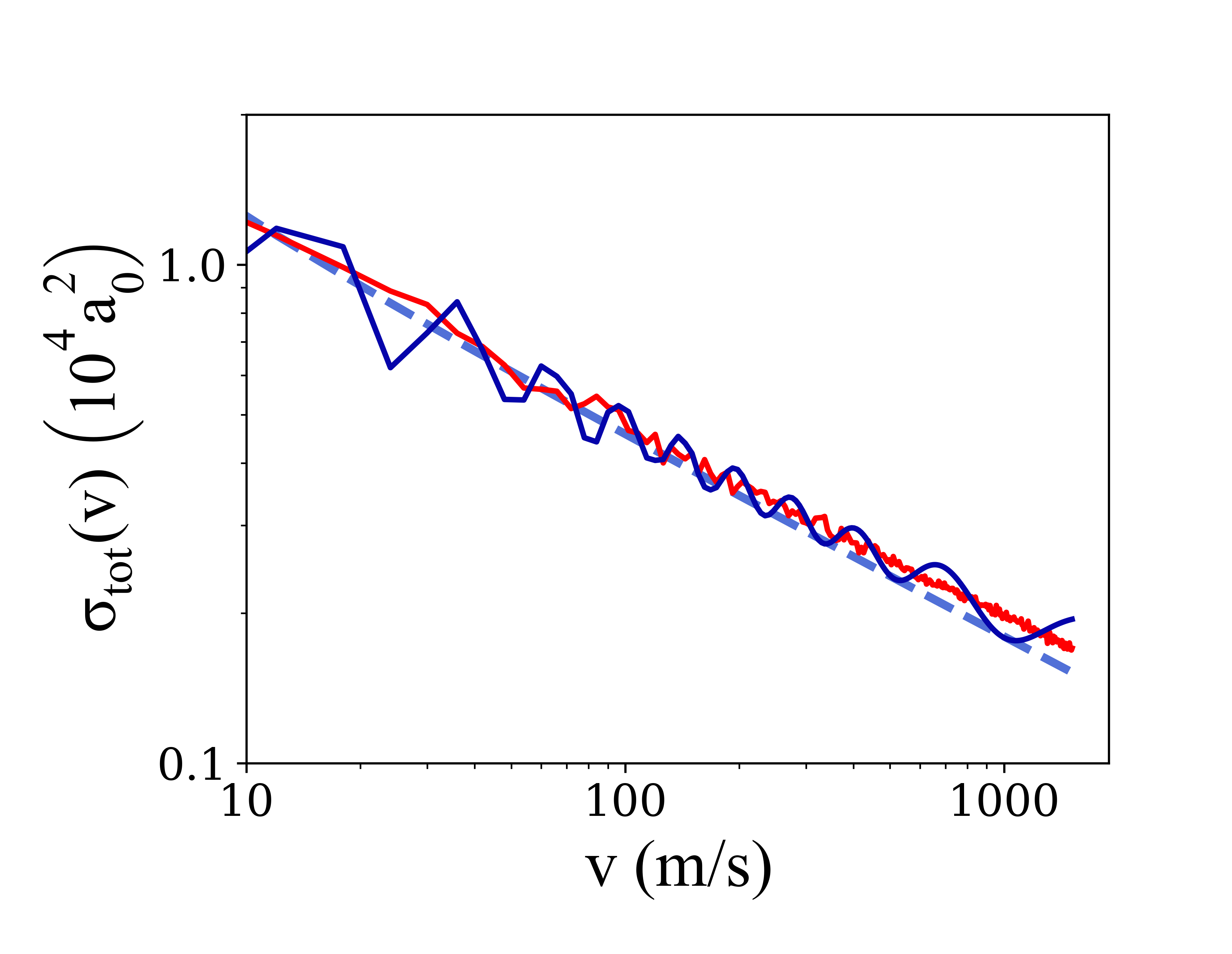
Figure 3: Plot of $\sigma_{\rm{tot}}(v)$ versus $v$ for FQMS computations based on the Kłos and Tiesinga [26] model interactions (blue trace), the purely $C_{6}$ model in Eq. 24 (blue dashed trace), and the SC model of Eq. 25 (red trace) for ⁸⁷Rb-Ar. The FQMS and SC predictions rise slightly above the pure $C_{6}$ predictions owing to the addition of the long-range $C_{8}$ and $C_{10}$ terms in these models. This leads to the $\left<\sigma_{\rm{tot}}\ v\right>$ value being systematically higher for a potential containing these terms than standard the LJ model.

To illustrate the effect of these omitted terms, Fig. 3 shows the ⁸⁷Rb-Ar total collision cross-section predictions, $\sigma_{\rm{tot}}(v)$, versus relative collision speed, $v$, based on the SC model (red solid trace) and the purely $C_{6}$ model (blue dashed trace) compared with those obtained from FQMS calculations using the Kłos and Tiesinga inter-species potentials [26] (blue solid trace).

The FQMS and SC predictions rise slightly above the pure $C_{6}$ predictions owing to the addition of the long-range $C_{8}$ and $C_{10}$ terms in these models. Notably, the SC model does not display any significant glory undulations, as the core portion of the potential responsible for these is absent. The undulatory FQMS $\sigma_{\rm{tot}}(v)$ values are centered around the SC values, underscoring that the role of the core repulsion is mainly confined to creating the glory oscillations over the range of $v<v^{\rm{max}}_{C6}$ depicted.

IV.2 Limitations of the Universality approximation

The minimization of the short range interaction potential influence on the collision rate coefficient is the result of velocity averaging for $v_{vdv}^{\rm{max}}<v^{\rm{max}}_{C6}$ which renders $\left<\sigma_{\rm{tot}}\ v\right>$ insensitive to the details of the glory undulations. The result is a value of $\left<\sigma_{\rm{tot}}\ v\right>$ which is well approximated by the SC estimate despite the SC model providing no account of the short range whatsoever. In the following, we examine the accuracy of the approximation, $\left<\sigma_{\rm{tot}}\ v\right>\simeq\left<\sigma_{\rm{tot}}\ v\right>_{\mathrm{SC}}$, for different sensor atoms and a variety of background gases.

We note at the outset of this discussion that the JB approximation upon which the SC phase shifts (and predictions) are based is not expected to be good at low velocities or small values of the angular momentum, $L$. However, the generic trend of $\sigma_{\rm{tot}}(v)$ seems to be captured by the SC model, and so the discrepancies of the $\left<\sigma_{\rm{tot}}\ v\right>$ and $\left<\sigma_{\rm{tot}}\ v\right>_{\mathrm{SC}}$ predictions will serve here as a heuristic indicator of universality. A full quantitative study of the actual insensitivity of $\left<\sigma_{\rm{tot}}\ v\right>$ to changes in the interaction potential (e.g. the values of $C_{6},\mu,D_{e}$) is the subject of future work.

Residual sensitivity to the interaction potential at short range and the resulting deviations of $\left<\sigma_{\rm{tot}}\ v\right>$ from $\left<\sigma_{\rm{tot}}\ v\right>_{\mathrm{SC}}$ are expected even when the velocity average is restricted to the universal regime, $v_{vdv}^{\rm{max}}<v^{\rm{max}}_{C6}$. These discrepancies are more significant when the glory undulations have a large amplitude and the velocity averaging does not encompass an integral number of undulations in the computation of $\left<\sigma_{\rm{tot}}\ v\right>$. For lower mass sensor atoms, the number of partial waves included in the computation of $\sigma_{\rm{tot}}(v)$ is reduced. As a result, the effects of glory scattering – which produce constructive or destructive interference centered around a partial wave, $L_{g}$ (see Appendix A) – have a relatively larger impact on the cross-section. This results in glory undulations with a larger amplitude. In addition, Bernstein [33, 34] and Child [30] assert that the number of glory undulations that appear in $\sigma_{\rm{tot}}(v)$ equals the number of rotation-less bound states that the inter-species potential can support. Lowering the reduced mass of the collision pair for a fixed potential depth lowers the number of these states, consequently reducing the number of glory oscillations in the $\sigma_{\rm{tot}}(v)$ versus $v$ spectrum. Both of these factors contribute to rendering the velocity averaging less effective in removing the influence of the glory scattering on the value of $\left<\sigma_{\rm{tot}}\ v\right>$.

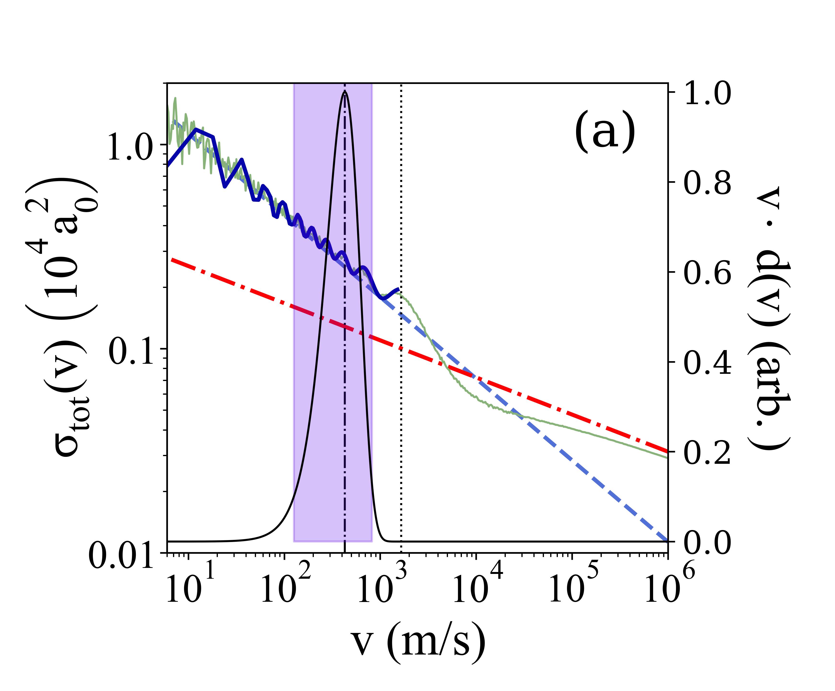
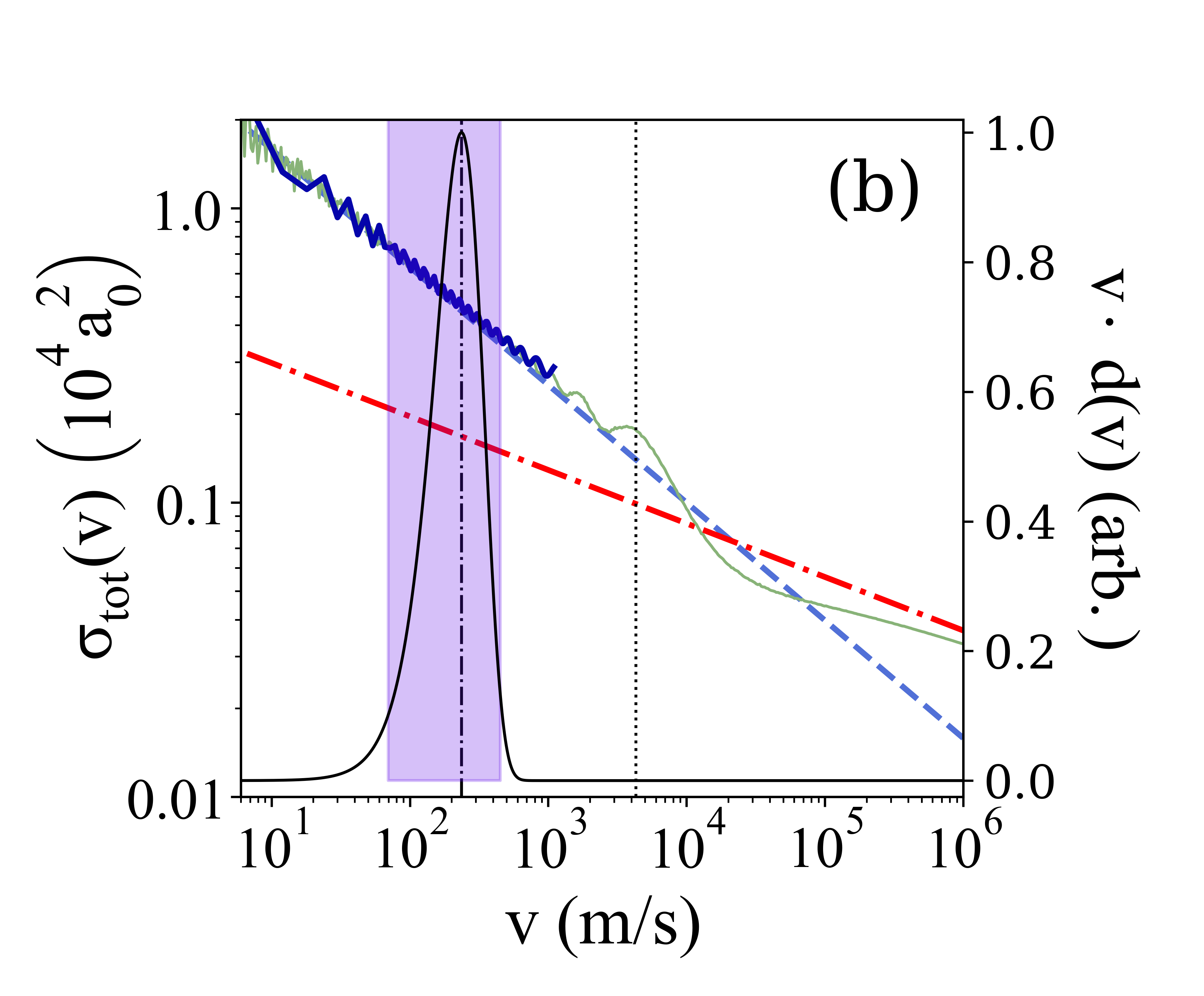
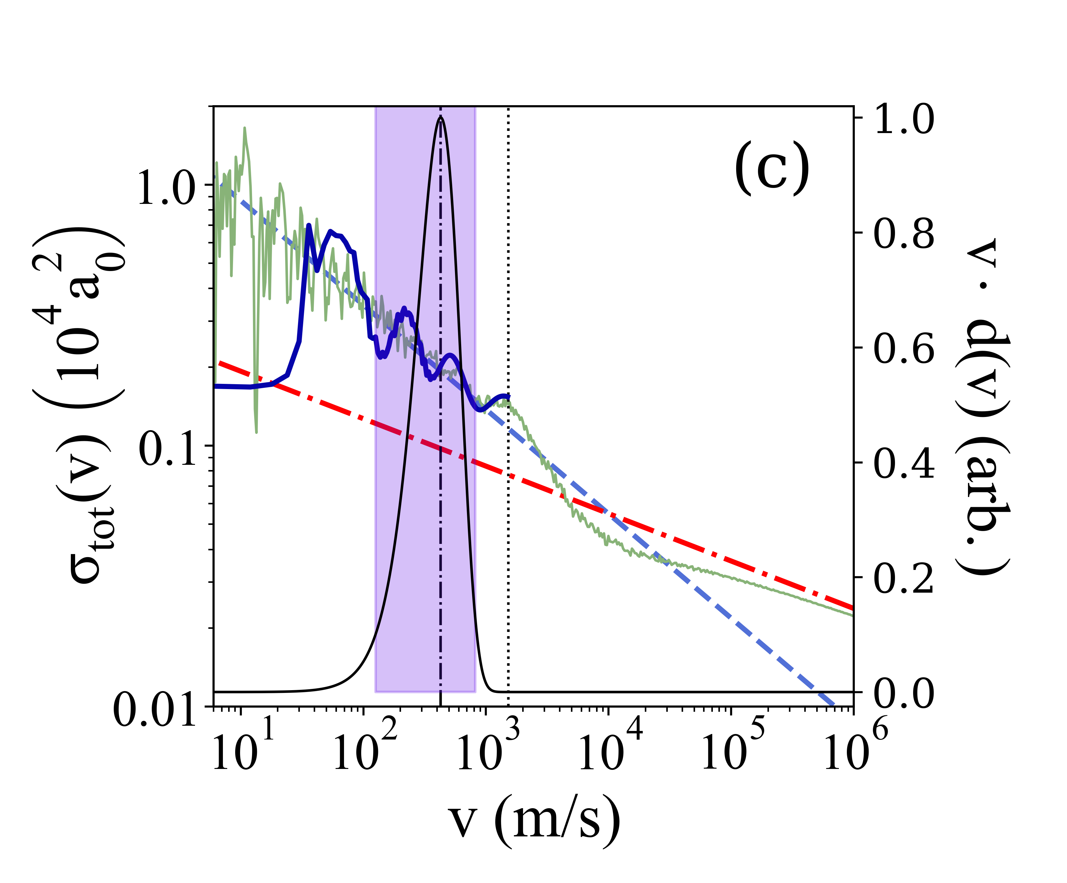
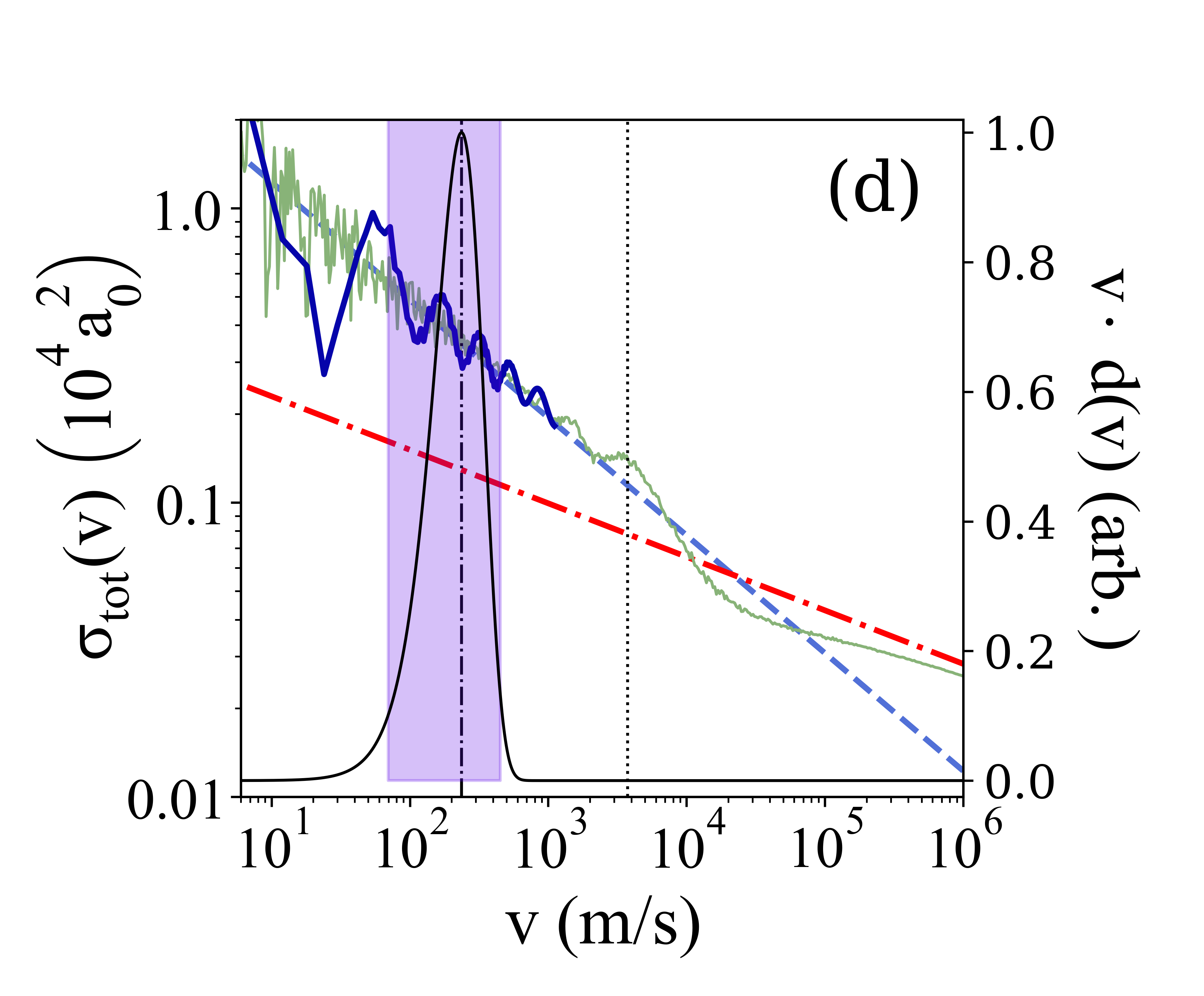
Figure 4: Plots of the $\sigma_{\rm{tot}}$ versus $v$ for (a) ⁸⁷Rb-Ar, (b) ⁸⁷Rb-Xe, (c) ⁷Li-Ar, and (d) ⁷Li-Xe for different interaction potential models. The cross section values are shown for FQMS computations using the KT potential [26] (thick blue traces), for a pure long-range $C_{6}$ potential, Eq. 18 (blue dashed traces), and for a pure short-range $C_{12}$ potential predictions, Eq. 20 (red dot-dashed traces). The thin green traces show $\sigma_{\rm{tot}}(v)$ computed using an augmented Lennard-Jones (a-LJ) potential which incorporates the $C_{8}$ and $C_{10}$ long-range van der Waals terms. The $C_{n}$ values values were taken from Kloss and Tiesinga (KT) [26] and the $C_{12}$ value was fixed to insure that the potential depth matched the KT potential value of $D_{e}$. Note how both the FQMS and modified LJ results rise above the purely $C_{6}$ predictions owing to the contributions of the $C_{8}$ and $C_{10}$ terms. As before, The black dotted vertical line indicates $v^{\rm{max}}_{C6}$, above which the cross-sections transition from long-range to short-range character. Also shown is the velocity weighted MB velocity distribution, $v\cdot d(v)$, (black line) with its maximum indicated by the vertical dash-dotted line for the room-temperature ($T=294$ K) background gas collision partner (Ar in (a) and (c), and Xe in (b) and (d)).

These effects are illustrated in Fig. 4. Figs. 4(a) and (b) depict the ⁸⁷Rb-Ar and ⁸⁷Rb-Xe $\sigma_{\rm{tot}}(v)$ vs $v$ values, respectively. These are contrasted by Fig. 4(c) and (d) which show the ⁷Li-Ar and ⁷Li-Xe computations, respectively. On each figure the FQMS computations (blue solid traces) based on the KT potentials [26], the purely $C_{6}$ predictions (blue dashed traces) and purely $C_{12}$ predictions (red dash-dot trace) are also shown. The green traces are the result of an augmented Lennard-Jones (a-LJ) potential model which includes the long-range $C_{8}$ and $C_{10}$ van der Waals terms (the Cn values were taken from [26]).

$$V_{\rm{a\text{-}LJ}}(r) = \frac{C_{12}}{r^{12}}-\frac{C_{10}}{r^{10}}-\frac{C_{8}}{r^{8}}-\frac{C_{6}}{r^{6}}.$$ (26)

The $C_{12}$ repulsive core coefficients were chosen such that the potential depths, $D_{e}$, equaled the values reported by by Klos and Tiesinga [26]. The cross-sections for this augmented LJ model were computed using the JB elastic phase shifts (Eqs. 19 and 25).

The FQMS computations appear to follow the a-LJ traces at large velocities where the JB approximation is expected to be good, and both rise above the purely $C_{6}$ prediction because they include the $C_{8}$ and $C_{10}$ long-range terms. This underscores the message of section IV.1 that the presence of the other long-range terms ($C_{8}$ and $C_{10}$) systematically increases the $\left<\sigma_{\rm{tot}}\ v\right>$ value above the $\left<\sigma_{\rm{tot}}v\right>_{\rm{C6}}$ prediction. In addition, it is clear that the ⁷Li-X (X = Ar or Xe) demonstrate fewer, larger amplitude glory undulations compared to their ⁸⁷Rb-X (X = Ar or Xe) counterparts. Thus, the corresponding $\left<\sigma_{\rm{tot}}\ v\right>$ values for ⁷Li-X cases are expected to exhibit a larger deviation from $\left<\sigma_{\rm{tot}}\ v\right>_{\mathrm{SC}}$, the predictions of the undulation-free SC model. The comparisons shown in Table 5 are consistent with this expectation.

To assess the validity of the universality approximation for ⁸⁷Rb-X collisions, FQMS computations of $\left<\sigma_{\rm{tot}}\ v\right>$ were carried out using the interaction potential models of Medvedev et al [38], furnishing $\left<\sigma_{\rm{tot}}\ v\right>_{\rm{Med}}$, and of Kłos and Tiesinga [26], providing $\left<\sigma_{\rm{tot}}\ v\right>_{\rm{KT}}$. Similarly, semi-classical (SC) values, $\left<\sigma_{\rm{tot}}\ v\right>_{\mathrm{SC}}$, were computed along with the purely $C_{6}$ predictions, $\left<\sigma_{\rm{tot}}v\right>_{\rm{C6}}$, Eq. 24. For all of these computations the MB averaging was carried out at an ambient temperature of 294 K. The results are presented in Table 4.

	($10^{-15}$m3/s)
Collision Pair	$\left<\sigma_{\rm{tot}}v\right>_{\rm{C6}}$	$\left<\sigma_{\rm{tot}}\ v\right>_{\rm{SC}}$	$\left<\sigma_{\rm{tot}}\ v\right>_{\rm{Med}}$	$\left<\sigma_{\rm{tot}}\ v\right>_{\rm{KT}}$
87Rb-He	2.49	3.07	2.44	2.37
87Rb-Ne	2.01	2.28	1.98	2.0
87Rb-Ar	2.81	3.00	3.04	3.03
87Rb-Kr	2.63	2.77	2.79	2.79
87Rb-Xe	2.75	2.87	2.88	2.87
87Rb-Rb	6.38	6.58	—	—

Table 4: A comparison of the computed $\left<\sigma_{\rm{tot}}\ v\right>$ values for ⁸⁷Rb-X (X = He, Ne, Ar, Kr, and Xe) at T = 294 K. The predictions based on FQMS calculations using the potentials from [38] are labeled $\left<\sigma_{\rm{tot}}\ v\right>_{\mathrm{Med}}$ and those obtained using the potentials from [26] are labeled $\left<\sigma_{\rm{tot}}\ v\right>_{\mathrm{KT}}$. The semi-classical predictions, $\left<\sigma_{\rm{tot}}\ v\right>_{\mathrm{SC}}$, are remarkably close to the FQMS predictions for the heavy collision partners although this SC calculation is based on the Jeffreys-Born approximation (Eq. 24) for the long-range induced scattering phase shifts and contains no information about the core repulsion of the potential. The purely $C_{6}$ predictions, $\left<\sigma_{\rm{tot}}v\right>_{\rm{C6}}$, are distinct from the $\left<\sigma_{\rm{tot}}\ v\right>_{\mathrm{SC}}$ predictions because the former does not include the phase shifts from the other long-range potential terms (i.e. the $C_{8}$ and $C_{10}$ terms). The final row shows the corresponding ⁸⁷Rb-Rb collision $C_{6}$ and SC values, based on the $C_{n}$ from [39].

For the universal pairs, ⁸⁷Rb-Ar, ⁸⁷Rb-Kr, and ⁸⁷Rb-Xe, the results are noteworthy: The $\left<\sigma_{\rm{tot}}\ v\right>_{\mathrm{Med}}$, $\left<\sigma_{\rm{tot}}\ v\right>_{\mathrm{KT}}$, and $\left<\sigma_{\rm{tot}}\ v\right>_{\mathrm{SC}}$ values are equivalent at the level of $<$ 1%. Because the KT and Med potentials are distinct at short range and because the SC calculation is devoid of any short range effects whatsoever, one concludes that the $\left<\sigma_{\rm{tot}}\ v\right>$ values for the universal pairs are independent of the interaction potential at short range due to MB averaging. In addition, the $\left<\sigma_{\rm{tot}}v\right>_{\rm{C6}}$ values are systematically lower than the corresponding $\left<\sigma_{\rm{tot}}\ v\right>_{\mathrm{Med}}$, $\left<\sigma_{\rm{tot}}\ v\right>_{\mathrm{KT}}$, and $\left<\sigma_{\rm{tot}}\ v\right>_{\mathrm{SC}}$ values. Clearly, the $C_{8}$ and $C_{10}$ values contribute a small, but non-negligible amount to the total collision cross-section coefficients (7% for ⁸⁷Rb-Ar, 5% for ⁸⁷Rb-Kr, 4% for ⁸⁷Rb-Xe, and 3% for ⁸⁷Rb-Rb). By contrast, the non-universal pairs, ⁸⁷Rb-He and ⁸⁷Rb-Ne, display large discrepancies between the SC predictions, $\left<\sigma_{\rm{tot}}\ v\right>_{\mathrm{SC}}$, and the FQMS physical model values ($\left<\sigma_{\rm{tot}}\ v\right>_{\mathrm{Med}}$ and $\left<\sigma_{\rm{tot}}\ v\right>_{\mathrm{KT}}$). Notably, the FQMS values also differ from each other due to the differences in their short range interaction potential while they have the same shape at long-range. This is a manifestation of the breakdown of universality for light collision partners as observed with direct measurements in 2023 [29].

To further investigate the universality approximation, $\left<\sigma_{\rm{tot}}\ v\right>$ was computed for Lithium-7 and Rubidium-87 sensor atoms colliding with H₂, He, Ne, N₂, Ar, Kr, and Xe by FQMS computations using the Kłos and Tiesinga (KT) model potentials [26] and by using the SC approximation, $\left<\sigma_{\rm{tot}}\ v\right>_{\mathrm{SC}}$, with the KT model $C_{n}$ values. The results are shown in Table 5.

	($10^{-15}$m3/s)		$\left<\sigma_{\rm{tot}}\ v\right>_{\rm{SC}}$
Collision Pair	$\left<\sigma_{\rm{tot}}\ v\right>_{\rm{KT}}$	$\left<\sigma_{\rm{tot}}\ v\right>_{\rm{SC}}$	$\mkern 1.5mu\overline{\mkern-1.5mu\left<\sigma_{\rm{tot}}\ v\right>_{\rm{KT}}\mkern-1.5mu}\mkern 1.5mu$
7Li-He	1.65	2.31	1.40
7Li-Ne	1.56	1.71	1.10
7Li-N2	2.63	2.62	0.996
7Li-Ar	2.33	2.31	0.991
7Li-Kr	2.14	2.12	0.991
7Li-Xe	2.24	2.20	0.982
87Rb-H2	3.89	5.89	1.51
87Rb-He	2.37	3.07	1.30
87Rb-Ne	2.00	2.28	1.14
87Rb-N2	3.45	3.45	1.000
87Rb-Ar	3.03	3.00	0.990
87Rb-Kr	2.78	2.77	0.996
87Rb-Xe	2.87	2.88	1.003

Table 5: A comparison of the computed $\left<\sigma_{\rm{tot}}\ v\right>$ values at T = 294K for ⁸⁷Rb-X and ⁷Li-X based FQMS calculations, $\left<\sigma_{\rm{tot}}\ v\right>_{\rm{KT}}$, using the Kłos and Tiesinga interaction potential from Ref. [26] to the semi-classical estimates, $\left<\sigma_{\rm{tot}}\ v\right>_{\rm{SC}}$, for X = H₂, He, Ne, N₂, Ar, Kr, and Xe. The final column gives the ratio of these two $\left<\sigma_{\rm{tot}}\ v\right>$ values. Remarkably, the SC predictions for ⁸⁷Rb - X and ⁷Li - X differ from the FQMS values by less than 1% and 2%, respectively, for the heavy collision partners, X = N₂, Ar, Kr, and Xe.

These computations demonstrate that the (universal) heavier collision partners, N₂, Ar, Kr, and Xe, yield $\left<\sigma_{\rm{tot}}\ v\right>$ values that agree with their corresponding semi-classical values, $\left<\sigma_{\rm{tot}}\ v\right>_{\mathrm{SC}}$. The ⁷Li-X (X = N₂, Ar, Kr) SC values are $<$ 1% larger than the $\left<\sigma_{\rm{tot}}\ v\right>_{\mathrm{KT}}$ and the ⁷Li-Xe is $<$ 2% larger. Similarly, the ⁸⁷Rb-X (X = N₂, Kr, Xe) values agree within 0.5%, and the ⁸⁷Rb-Ar within 1%. Thus, the ansatz that the $\left<\sigma_{\rm{tot}}\ v\right>$ values are independent of the details of the core potentials appears to be supported for both ⁷Li and ⁸⁷Rb sensor atoms. For the lighter collision partners examined, H₂, He, and Ne, the center of their $v\cdot d(v)$ distribution, $v_{vdv}^{\rm{max}}$, lies above the estimated long range dominated velocity limit, $v_{\rm{C6}}^{\rm{max}}$. The result is that these $\left<\sigma_{\rm{tot}}\ v\right>$ carry information about the core repulsion, providing an opportunity to refine the model potentials against directly measured quantities.

V Revising $p_{\rm{QDU}}$

The trap loss rate coefficient, $\left<\sigma_{\rm{loss}}\ v\right>$ (Eq. 11), was previously studied using FQMS calculations with a LJ interaction potential and was found to be insensitive to the shape of the interaction potential at short range. The shape of $\left<\sigma_{\rm{loss}}\ v\right>/\left<\sigma_{\rm{tot}}\ v\right>$ was then fit to a polynomial whose coefficients are provided in Table 2. Because the LJ model used lacks the $C_{8}$ or $C_{10}$ long-range terms, the validity of this prior analysis is suspect. To investigate this further, FQMS computations of $\left<\sigma_{\rm{loss}}\ v\right>$ were carried out using the more realistic Kłos and Tiesinga (KT) potential model [26], the LJ model, and the SC model, which lacks any short range portion, for the universal collision pairs ⁸⁷Rb-Ar and ⁸⁷Rb-Xe. From Eq. 11, we have,

$$\frac{\left<\sigma_{\rm{loss}}\ v\right>}{\left<\sigma_{\rm{tot}}\ v\right>}=1-p(U).$$ (27)

The ratios are shown in Fig. 5 for these universal collision pairs. While the shapes of the $1-p(U)$ versus $U$ curves differ for the different collision pairs, ⁸⁷Rb-Ar and ⁸⁷Rb-Xe, the shapes for each pair are independent of the collision model used, for shallow traps. That is, for ⁸⁷Rb-Ar the values for the SC model (red diamonds) and the LJ model (white triangles) overlap the realistic KT model (grey dotted trace). Similarly, the SC model (violet diamonds) and LJ model (white triangles) values overlap the KT model (grey dotted trace) for ⁸⁷Rb-Xe in Fig. 5(b).

Thus, one concludes that $p(U)$ depends on the collision pair but does not depend on the collision model employed in the FQMS. Of key importance is that this comparison shows that $p(U)$ does not depend on the presence of the $C_{8}$ and $C_{10}$ terms in the potential since they are completely absent for the LJ model, nor does it depend on the details of the core of the potential, as the SC model does not have any repulsive core. By contrast, the value of $\left<\sigma_{\rm{tot}}\ v\right>$ definitely depends on these $C_{8}$ and $C_{10}$ terms for these universal collision pairs (as discussed in section IV.1).That the three models, sharing only the same long range $C_{6}$ behavior, predict the same curve yet have distinct total cross sections leads to the prediction that the universal function, $p(U)$, previously defined purely on the basis of the LJ model computations (Eq. 15) should persist for these species (⁸⁷Rb-Ar, ⁸⁷Rb-Kr, and ⁸⁷Rb-Xe), but requires a key modification,

$$p(U)=p_{\rm{QDU,6}}=\sum_{j}\beta_{j}\left(\frac{U}{U_{d,6}}\right)^{j}.$$ (28)

Here,

$$U_{d,6}=\frac{4\pi\hbar^{2}}{m_{t}\left<\sigma_{\rm{tot}}v\right>_{\rm{C6}}/v_{p}}$$ (29)

and $\left<\sigma_{\rm{tot}}v\right>_{\rm{C6}}$ is the total collision cross-section coefficient based solely on the $C_{6}$ interaction, Eq. 24. This formulation updates the energy scaling for the normalized trap loss rate to one that only depends on the long-range $C_{6}$ behavior instead of the total collision rate coefficient. To illustrate this, Figure 6 shows the same FQMS data sets but now $\left<\sigma_{\rm{loss}}\ v\right>/\left<\sigma_{\rm{tot}}\ v\right>=1-p(U)$ is plotted versus the scaled trap depth, $U/U_{d,6}$. Both the KT model FQMS computations and the LJ values converge to the same universal shape.

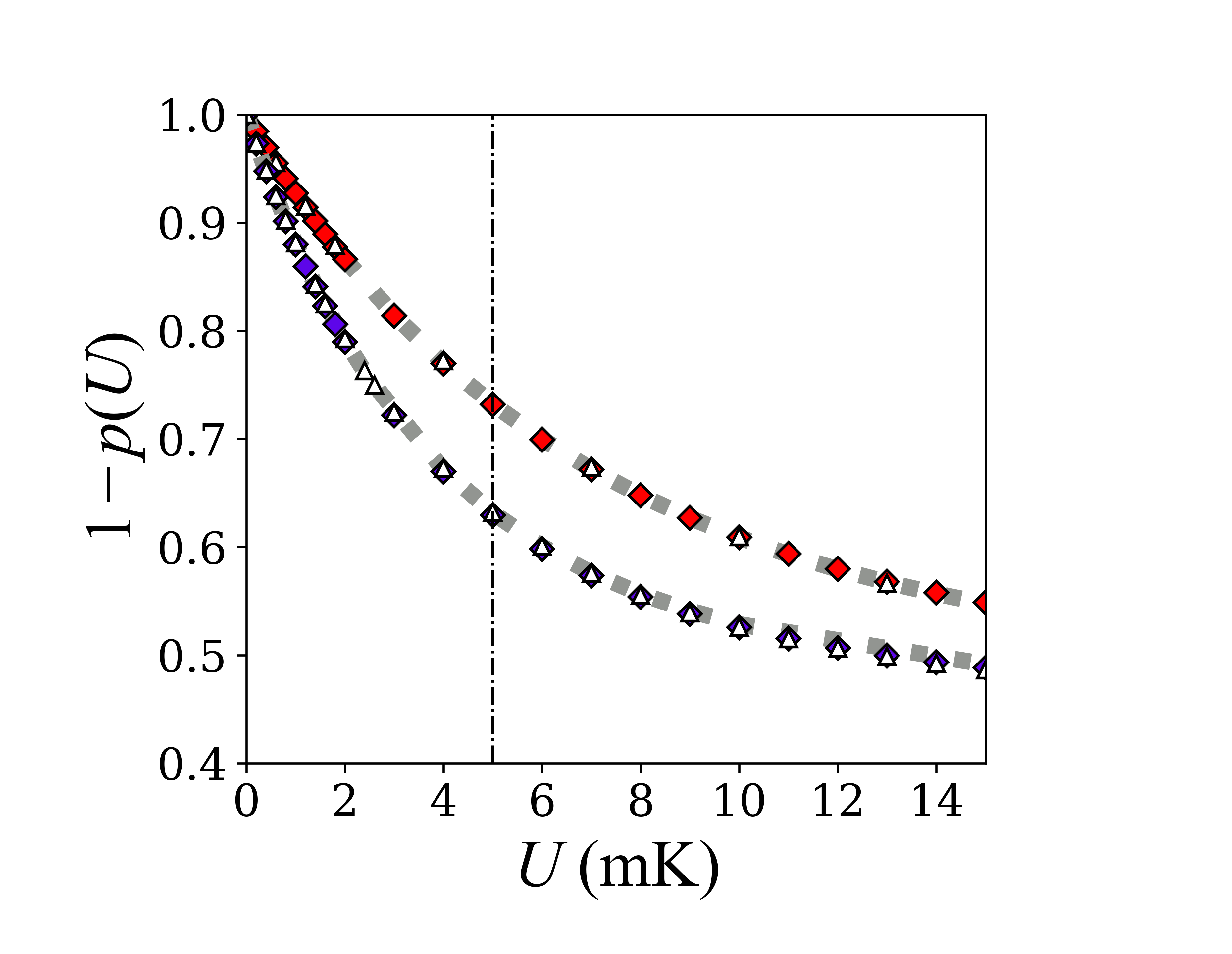
Figure 5: A plot of $\left<\sigma_{\rm{loss}}\ v\right>/\left<\sigma_{\rm{tot}}\ v\right>=1-p(U)$ versus trap depth, $U$ for collisions between ⁸⁷Rb and the heavy (universal) partners, Ar and Xe, at T = 294K. The grey dotted traces are the FQMS prediction using the Klos and Tiesinga (KT) potetial [26] for ⁸⁷Rb-Ar (upper trace) and for ⁸⁷Rb-Xe (lower trace). The SC prediction model for ⁸⁷Rb-Ar is shown as red diamonds, and the SC prediction for ⁸⁷Rb-Xe is shown as the violet diamonds. Overlaid on these are the corresponding FQMS predictions for the LJ model (white triangels). Note how the ⁸⁷Rb-Ar and ⁸⁷Rb-Xe predictions are clearly distinct, but the predictions from using different interaction potentials overlap well over this range of trap depths, indicating that they yield the same $p(U)$. The vertical dot-dashed lines are the maximum achievable $U/U_{\rm{d},6}$ attained thus far in experiments.

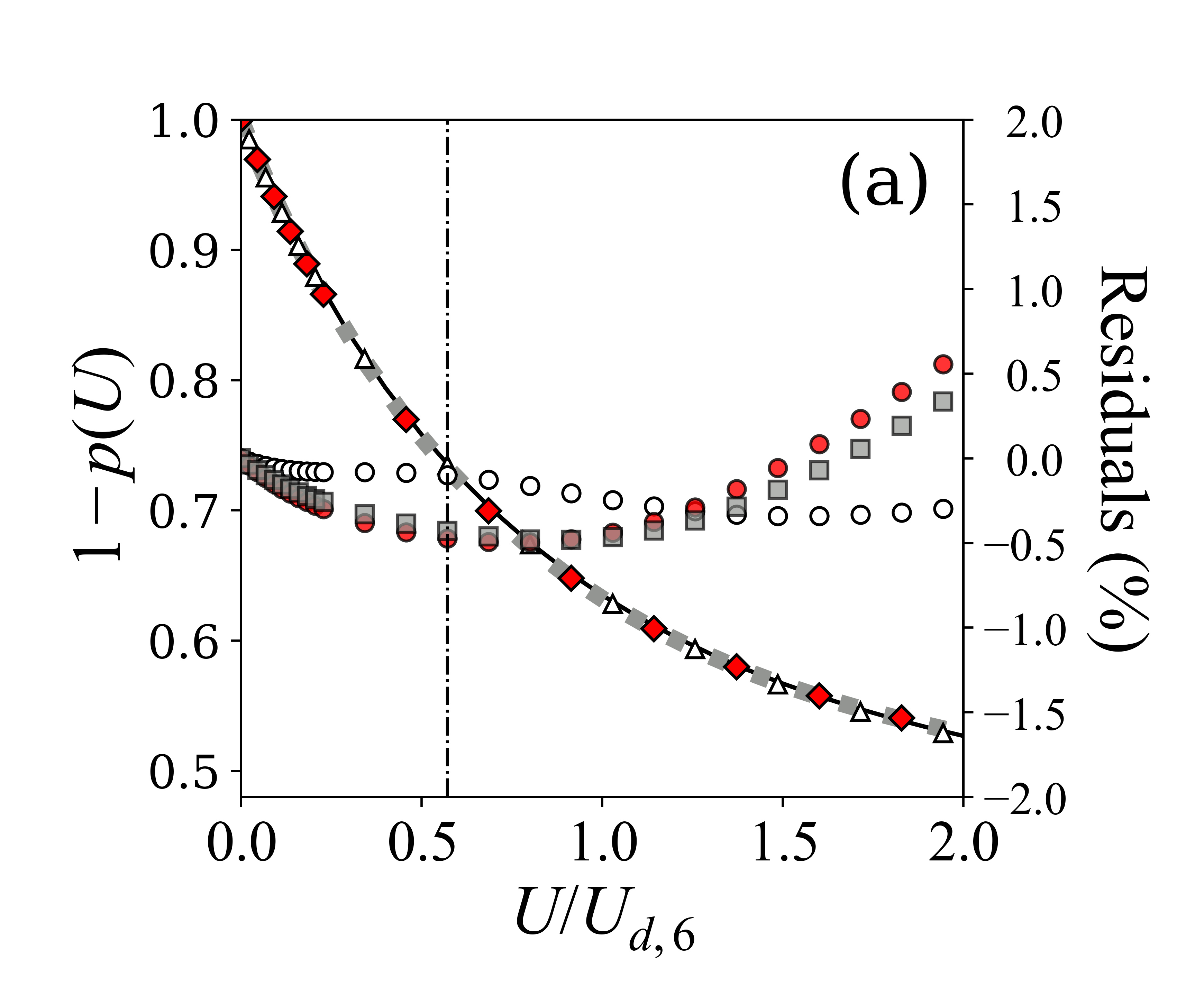
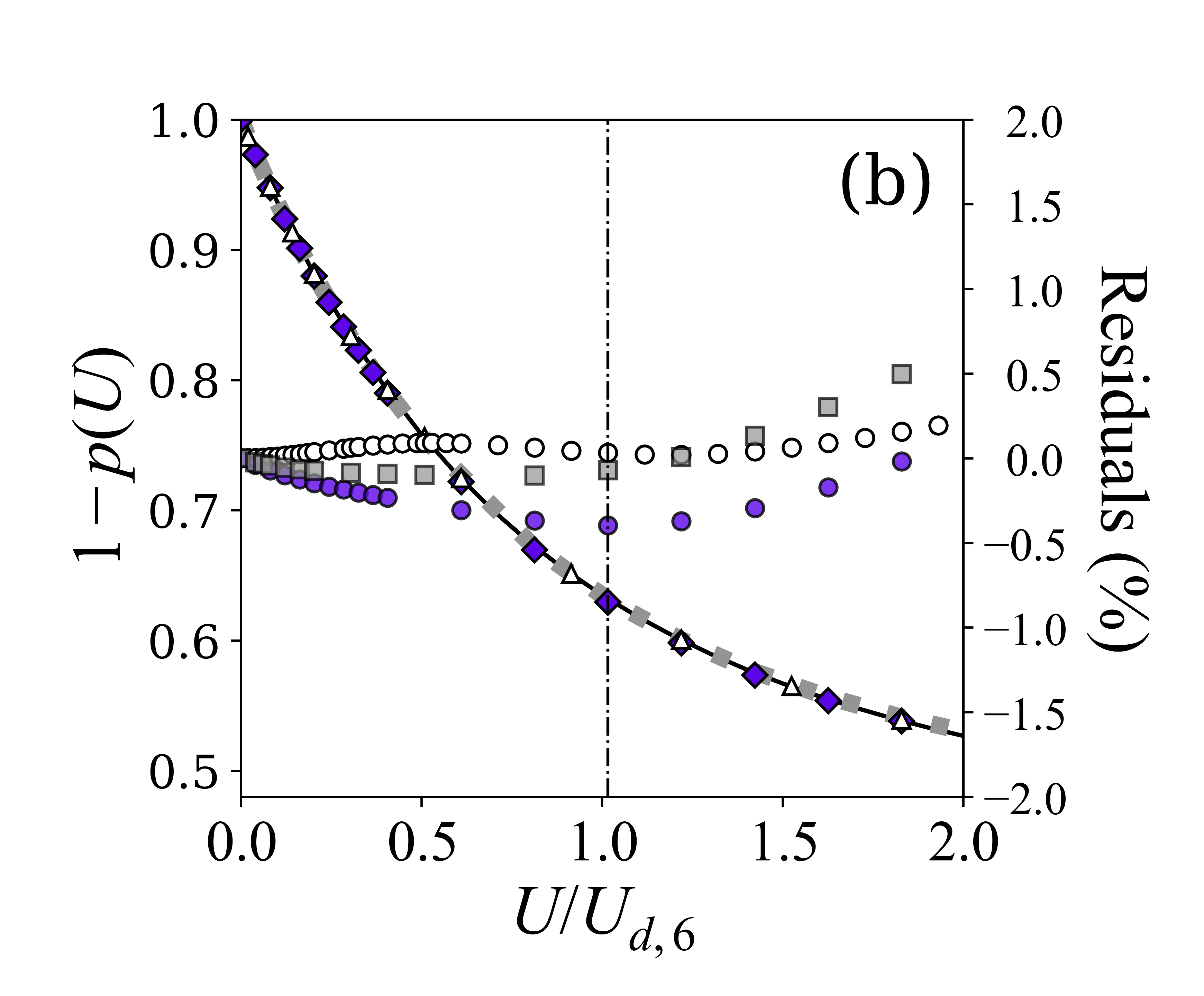
Figure 6: Plots of $\left<\sigma_{\rm{loss}}\ v\right>/\left<\sigma_{\rm{tot}}\ v\right>=1-p(U)$ versus the scaled trap depth, $U/U_{\rm{d},6}$, using different potential models for collisions between ⁸⁷Rb and Ar between ⁸⁷Rb and Xe (universal species) at T = 294 K. The overlap between the predictions is remarkable: (a) shows ⁸⁷Rb-Ar FQMS values based on the Klos and Tiesinga (KT) model (dotted gray trace), the SC model (red diamonds), and the LJ model (white triangles). (b) shows the ⁸⁷Rb-Xe KT model (dotted grey trace), SC model (violet diamonds), and LJ model (white triangles). The universal predictions are shown in both figures as the solid black trace. The percent residuals between the different models and the universal expression, Eq. 28, are plotted as individual points on each figure: KT model as grey squares, SC model as red circles for ⁸⁷Rb-Ar and violet circles for ⁸⁷Rb-Xe, while the white circles are the LJ residuals on both plots. The vertical dot-dashed lines are the maximum achievable $U/U_{\rm{d},6}$ attained thus far in experiments.

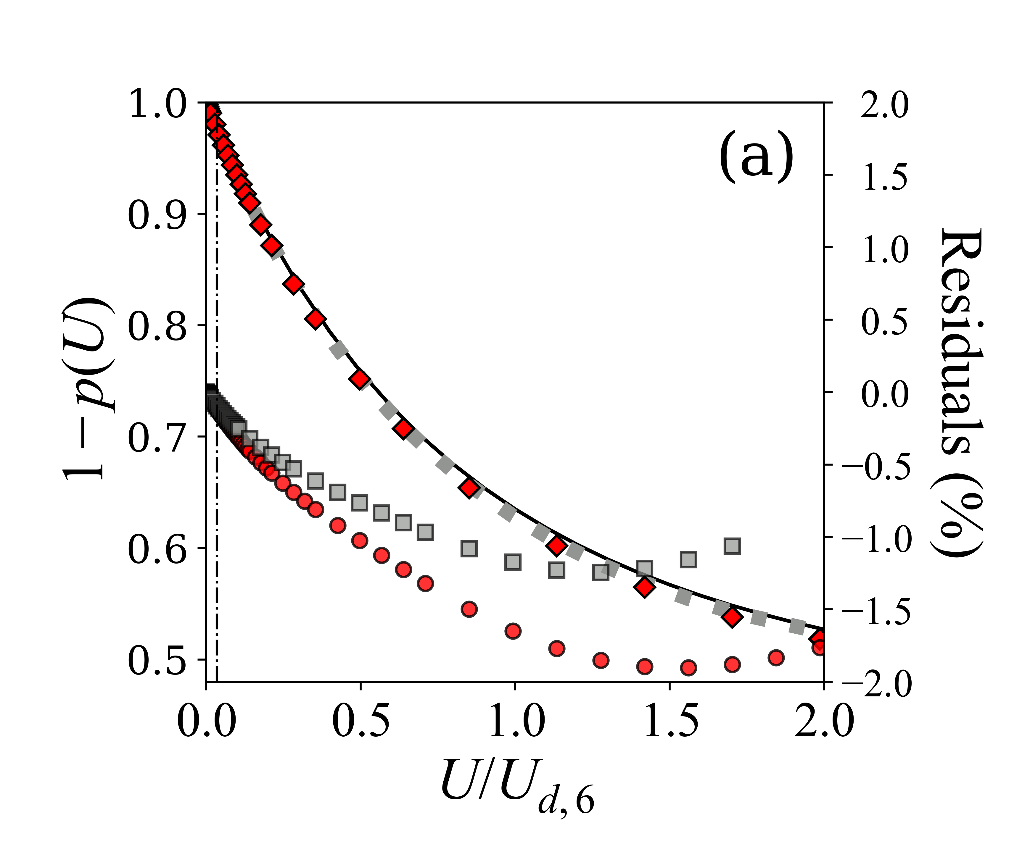
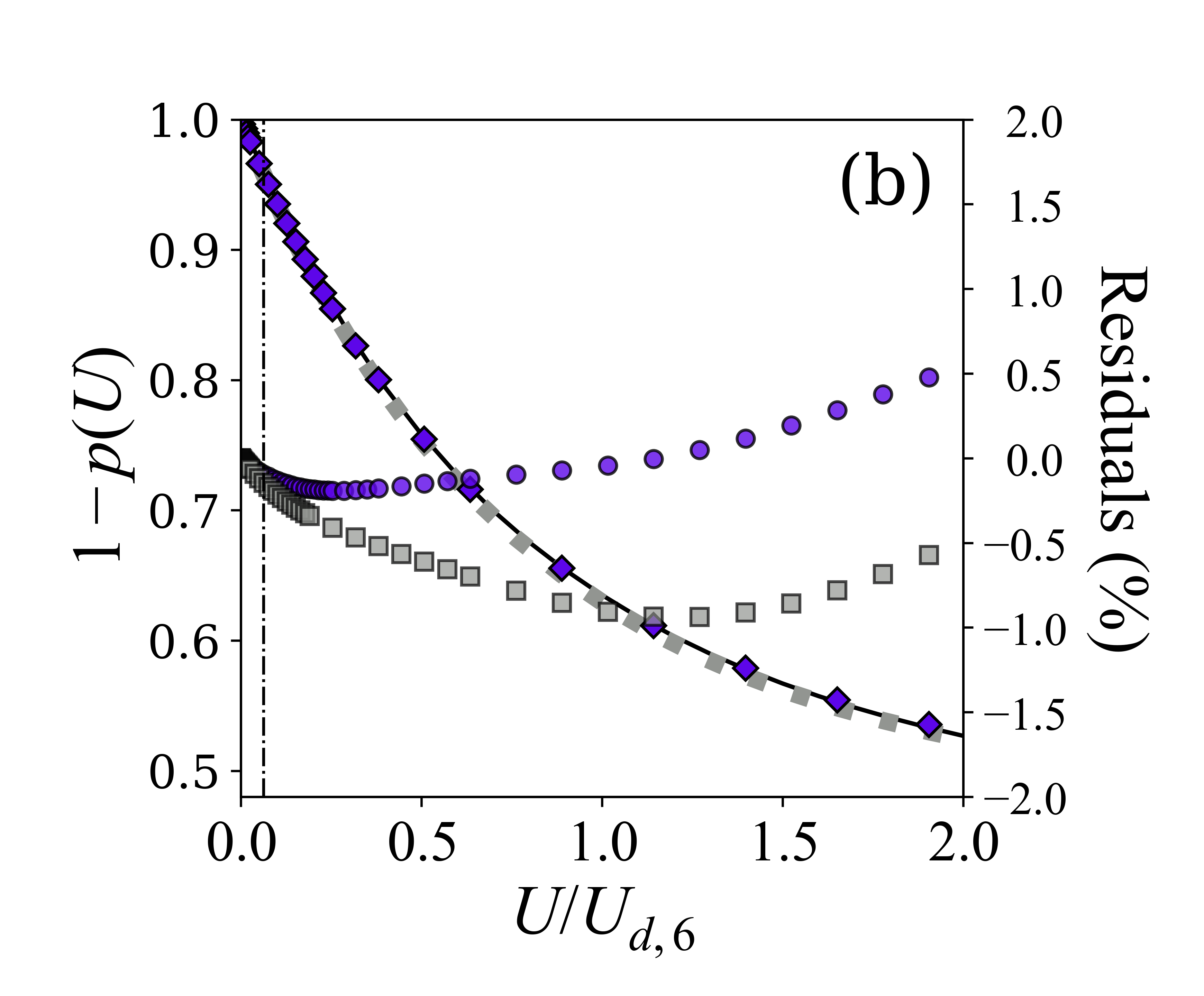
Figure 7: Plots of $\left<\sigma_{\rm{loss}}\ v\right>/\left<\sigma_{\rm{tot}}\ v\right>=1-p(U)$ versus $U/U_{d,6}$ for (a) ⁷Li-Ar and (b) ⁷Li-Xe. In (a) the dotted grey trace is the FQMS prediction based on the KT model and the red diamonds are the SC model values. The percent residuals between the KT model and universal predictions (grey squares) and between the SC model and universal predictions (red circles). Plot (b) shows the ⁷Li-Xe KT FQMS values (grey dotted trace) and the SC model predictions (violet diamonds). In addition the residuals between the KT FQMS values and the universal predictions (grey squares) and between the SC model and the universal model (violet circles) are plotted. The solid black traces are the universal predictions. These plots underscore that the normalized variation of $\left<\sigma_{\rm{loss}}\ v\right>/\left<\sigma_{\rm{tot}}\ v\right>$ as a function of $U$ is determined primarily by the long range $C_{6}/r^{6}$ portion of the interaction potential for shallow traps. The vertical dot-dashed lines are the maximum achievable $U/U_{\rm{d},6}$ attained thus far in experiments.

We find that this updated universal expression for the trap loss rate, Eq. 28, leads to discrepancies with the KT FQMS values and the SC values which are less than 0.5% for $U/U_{\rm{d},6}\leq 1.0$ for ⁸⁷Rb-Ar and ⁸⁷Rb-Xe collisions. The $U_{\rm{d},6}$ model was also applied to ⁷Li-Ar, ⁷Li-Kr, and ⁷Li-Xe collision pairs (Fig. 7(a) and (b) show the ⁷Li-Ar and ⁷Li-Xe results). In these cases we observe that the KT FQMS residuals with the universal predictions are systematically negative, up to -1.0%, while the SC model residuals are also systematically negative, up to -1.7% over the same $U/U_{\rm{d},6}\leq 1.0$ range. The ⁷Li-Xe demonstrate the same systematic negative residual between the KT FQMS and universal predictions, while the SC model residuals with the universal function vary from -0.2% to 0.5%. We limit the range for this consideration out to $U/U_{\rm{d},6}\leq 1.0$ because we are using a truncated polynomial approximation to the universal function, and its accuracy is expected to worsen for $U/U_{\rm{d},6}>1.0$. This is evident in Fig. 6 where the discrepancies grow past $U_{\rm{d},6}$. While the SC and KT FQMS predictions are extremely close for ⁸⁷Rb-X collisions, there is a larger discrepancy between them for ⁷Li-X. The JB approximation is less accurate for lower $L$ collisions, consequently, the SC approximation will be less accurate for ⁷Li-X collisions as there are fewer partial waves at play in the collisions. As can be seen in Fig. 8, $\sigma(v\simeq v_{\rm{p}})$ has significant contributions for partial waves up to $L=35$ for ⁷Li-Ar versus $L=175$ for ⁸⁷Rb-Ar. The remaining (small amplitude) structure of the FQMS residuals is distinct for each collision pair suggesting that the normalized trap loss rate may not be completely determined by $C_{6}$ alone; however, understanding the exact origin of these differences is beyond the scope of this work.

The interpretation of the normalized trap rate variation with trap depth following a universal curve is that quantum diffractive collisions, which impart very little momentum and energy to the trapped ensemble and contribute to sensor atoms being retained at small ($<1$ mK) trap depths, primarily probe the long range $-C_{6}/r^{6}$ portion of the interaction potential. In the classical sense, these collisions correspond to very large impact parameter collisions and thus only probe the interaction potential at extremely long range.

Because $p(U)$ for shallow traps ($U\leq U_{\rm{d},6}$) only depends on $U_{d,6}$, the atom sensor is not self-calibrating as originally conceived. That is, fitting the experimentally measured loss rate ratio, $\Gamma_{\rm{loss}}(U)/\Gamma_{\rm{loss}}(U=0)$ at a fixed background gas pressure for different trap depths, $U$, to Eq. 28 will yield $\left<\sigma_{\rm{tot}}v\right>_{\rm{C6}}$ rather than $\left<\sigma_{\rm{tot}}\ v\right>$. Indeed, recent work studying ⁸⁷Rb-Rb collisions which extracted the $C_{6}$ value from trap loss measurements, supports this assertion [28]. In addition, the experimentally determined $\left<\sigma_{\rm{tot}}\ v\right>$ values from [14] also support this interpretation, as illustrated in Table 6.

	($10^{-15}$m3/s)
Collision Pair	$\left<\sigma_{\rm{tot}}\ v\right>_{\rm{KT}}$[26]	$\left<\sigma_{\rm{tot}}v\right>_{\rm{C6}}$	$\left<\sigma_{\rm{tot}}\ v\right>_{\rm{QDC}}$[14]
87Rb-H2	3.9(1)	4.98	5.12(15)
87Rb-He	2.37(3)	2.49	2.41(14)
87Rb-Ne	2.0(2)	2.01	—
87Rb-N2	3.45(6)	3.18	3.14(5)
87Rb-Ar	3.035(7)	2.81	2.79(5)
87Rb-Kr	2.79(1)	2.63	—
87Rb-Xe	2.88(1)	2.75	2.75(4)
87Rb-Rb [28]	—	6.38	6.44(12)

Table 6: A comparison of the $\left<\sigma_{\rm{tot}}\ v\right>$ values for ⁸⁷Rb-X (X = H₂, He, Ne, N₂, Ar, Kr, and Xe) at T = 294K. The second column shows the FQMS values from Ref.[26], the third shows the purely $C_{6}$ potential predictions, $\left<\sigma_{\rm{tot}}v\right>_{\rm{C6}}$, and the final column gives the values derived from fitting the universal model (Eq. 28) for trap loss to experimental measurements, $\left<\sigma_{\rm{tot}}\ v\right>_{\rm{QDC}}$, reported in [14]. Also included is the result from [28] for ⁸⁷Rb-Rb collisions. The good agreement between the $\left<\sigma_{\rm{tot}}v\right>_{\rm{C6}}$ and the $\left<\sigma_{\rm{tot}}\ v\right>_{\rm{QDC}}$ for heavy collision pairs is experimental evidence supporting the revised hypothesis that the trap loss rate variation with trap depth depends only on $\left<\sigma_{\rm{tot}}v\right>_{\rm{C6}}$ and not $\left<\sigma_{\rm{tot}}\ v\right>$ as originally conjectured.

Because of the presence of the long range $C_{8}$ and $C_{10}$ terms, which systematically increase the total rate coefficient, the purely experimental calibration procedure of extracting $U_{d}$ from measurements of trap loss rates will lead to an estimate of the rate coefficient that is systematically lower than the true value, $\left<\sigma_{\rm{tot}}v\right>_{\rm{C6}}<\left<\sigma_{\rm{tot}}\ v\right>$. As discussed above, this discrepancy is up to 7% (for ⁸⁷Rb-Ar) collisions. When the $C_{6}$, $C_{8}$, and $C_{10}$ coefficients are known a priori, then the semi-classical approximation for the elastic scattering phase shifts offers an opportunity to determine a more accurate estimate of $\left<\sigma_{\rm{tot}}\ v\right>$.

VI Conclusions

Using full quantum mechanical scattering calculations and realistic interaction potentials taken from Refs. [26, 38], we have re-examined the original postulates of the universality hypothesis for room-temperature collisions reported in [12, 13]. We find evidence supporting the hypothesis that the total collision rate coefficient, $\left<\sigma_{\rm{tot}}\ v\right>$, and the trap loss rate coefficient, $\left<\sigma_{\rm{loss}}\ v\right>$, are universal for heavy collision partners with either a heavy (⁸⁷Rb) or a light (⁷Li) sensor atom, determined solely by the long-range portion of the inter-species interaction potential.

This universality of $\left<\sigma_{\rm{tot}}\ v\right>$ for room-temperature collisions is particularly significant to vacuum metrology because it implies that errors or uncertainties in the short-range part of the interaction potential do not propagate to the total collision rate coefficient and thus to the density or pressure inferred from a measurement.

For such universal collision partners, the total rate coefficient, $\left<\sigma_{\rm{tot}}\ v\right>$, is well approximated by a semi-classical prediction, $\left<\sigma_{\rm{tot}}\ v\right>_{\mathrm{SC}}$, that only accounts for the scattering phase shift arising from the long-range interaction potential terms, $C_{6}$, $C_{8}$, and $C_{10}$. Specifically the values of $\left<\sigma_{\rm{tot}}\ v\right>$ found by FQMS calculations using the KT potentials were found to agree with the $\left<\sigma_{\rm{tot}}\ v\right>_{\mathrm{SC}}$ predictions to better than 0.5% for ⁸⁷Rb-(N₂, Ar, Kr, Xe) collisions and to within 1% for ⁷Li-(N₂, Ar, and Kr), and within 2% for ⁷Li-Xe. The bigger discrepancy observed for collisions with ⁷Li sensor atoms is attributed to the larger amplitude and lower frequency (in $v$ or $k=\mu v/\hbar$) glory oscillations in the total quantum mechanical cross-sections, $\sigma_{\rm{tot}}(v)$, associated with the smaller reduced mass for these pairs. For these cases, the averaging over the ambient temperature Maxwell-Boltzmann distribution of the background collisions inherent in the $\left<\sigma_{\rm{tot}}\ v\right>$ coefficient does not completely suppress the glory effects.

We also confirm the previously reported breakdown of this collision universality for light background gas collision partners. The breakdown is due the room temperature velocity average extending above $v^{\rm{max}}_{C6}$ where the shape of $\sigma_{\rm{tot}}(v)$ is dominated by the shape of the interaction potential at short range. Another feature of light background gas collision partners is that the shape of $\sigma_{\rm{tot}}(v)$ does not have a significant domain in relative speed where it follows the purely long-range character prediction.

Finally, we study the variation of the loss rate coefficient with trap depth for universal collision pairs and find that while $\left<\sigma_{\rm{tot}}\ v\right>$ (equivalently $\left<\sigma_{\rm{loss}}\ v\right>(U=0)$) depends on all of the long range terms ($C_{6}$, $C_{8}$, and $C_{10}$), the shape of the normalized trap loss rate coefficient ($\left<\sigma_{\rm{loss}}\ v\right>(U)/\left<\sigma_{\rm{tot}}\ v\right>$), for small trap depths, only provides information about the leading order interaction potential term, $-C_{6}/r^{6}$. The consequence is that a fit of the experimentally measured loss rates normalized by the loss rate at zero trap depth will provide the energy scale $U_{\rm{d},6}$ and the corresponding $\left<\sigma_{\rm{tot}}v\right>_{\rm{C6}}$ instead of the total collision rate coefficient as originally postulated in [12, 13]. This finding together with the fact that the total collision rate coefficient for universal collision pairs is increased by the presence of the $C_{8}$ and $C_{10}$ long range terms implies that sensor atom self-calibration will provide an estimate, $\left<\sigma_{\rm{tot}}v\right>_{\rm{C6}}$, which is systematically below $\left<\sigma_{\rm{tot}}\ v\right>$ by up to approximately 10% (as shown in Tab. 6). Finally, the expectation is that the variation of the normalized loss rate coefficient with trap depth for a non-universal collision pair will deviate from the universal function and will depend on the entire interaction potential.

We believe these findings explain the observed discrepancies, reinforce the conjecture that room-temperature collisions are universal, insensitive to the short range interaction potential shape, and offer immediate implications for using atoms as a self-calibrating primary pressure standard.

VII Acknowledgements

We acknowledge the financial support from the Natural Sciences and Engineering Research Council of Canada (NSERC grants RTI-2016-00120, RGPIN-2019-04200, RGPAS-2019-00055) and the Canadian Foundation for Innovation (CFI project 35724). This work was done at the Center for Research on Ultra-Cold Systems (CRUCS) and was supported, in part, through computational resources and services provided by Advanced Research Computing at the University of British Columbia.

Appendix A Glory Oscillation Origins and Predictions

Universality relies on velocity averaging to minimize or eliminate the effects of the glory undulations inherent in the elastic scattering process. When successful, the averaging reveals the nature of the long-range potential while erasing any information about the short-range portion of the inter-species interaction.

In this appendix we illustrate the origins of the glory undulations seen in the $\sigma_{\rm{tot}}(v)$ versus $v$ spectrum as an aid to define the limits of validity of the universality hypothesis. In particular, we use a Lennard-Jones (LJ) potential to derive the salient features of the glory oscillations. Namely,

1. We use the Jeffreys-Born approximation for the phase shifts to determine the partial wave which leads to glory scattering, $L_{g}$, for each $v$.

2. Based on the analysis of Bernstein[33, 34] the upper limit of the speed over which the long-range portion of the potential dominates the $\sigma_{\rm{tot}}(v)$ values, $v^{\rm{max}}_{C6}$, is estimated.

3. Using an expression from [34] the number of bound states the inter-species potential can support is computed and provides an estimate for the number of glory undulations observed over the cross-section spectrum [30, 34] up to $v\approx v^{\rm{max}}_{C6}$.

4. We compare the partial wave dependencies of the cross-sections for ⁸⁷Rb-Ar to ⁷Li-Ar to demonstrate how the lighter trapped species leads to larger amplitude glory undulations.

5. Finally we provide an upper limit estimate of the maximum expected glory undulations-induced deviation to the values of the total collision coefficients, $\left<\sigma_{\rm{tot}}\ v\right>$.

For the rest of this appendix we will use a LJ potential to describe the inter-species collisions. While this is not a physically realistic potential, it allows us to derive tractable results which capture the behavior observed in FQMS calculations using more realistic potentials.

A.1 Glory Oscillations

Glory undulations in the cross-section occur when lower - $L$ partial waves scatter in the forward direction ($\theta=0$) and interfere with the large-$L$ partial waves which are also primarily scattered in the forward direction. To illustrate this phenomenon, plots of $\sigma(v,L)$ versus $L$ for ⁸⁷Rb-Ar collisions at $T=294$ K for a LJ potential are shown in Fig. 8 for several collision speeds.

$$\sigma(k,L) = \frac{4\pi}{k^{2}}\left(2L+1\right)\sin^{2}\eta_{L}(k).$$ (30)

One observes that $\sigma(k,L)$ has a characteristic shape consisting of a lower-$L$ regime where it oscillates rapidly, corresponding to the rapid change in $\eta_{L}(k)$ (or, equivalently $\eta_{L}(v)$) with $L$. This is followed by a final lobe for which $0\leq\eta_{L}(k)\leq\pi$. The peak of this lobe occurs at $\eta_{L}(k)\approx\pi/2$.

In the absence of glory scattering, these plots would all look similar, with $\sigma(k,L)$ oscillating smoothly as the maxima grow monotonically following the $(2L+1)$ asymptote out to the final lobe. Glory scattering introduces interference which can reinforce or suppress the contributions of a small range of partial waves centered at the value $L_{g}$. Such interference is evident in the plots in Fig. 8 with the approximate value of $L_{g}$ shown by the red arrows. (Fig. 8(a) demonstrates strong destructive interference, while (b) displays constructive interference.) The values of $\sigma_{\rm{tot}}(v)$ plotted in Figs. 2, 3 and 6, are the sum of these $\sigma(k,L)$. Thus, the glory undulations arise from the interference effects deviating the sum from the underlying, monotonic long-range prediction (e.g. Eq. 24 for a purely $C_{6}$ potential).

For elastic collisions [30] we can relate the scattering angle to the elastic scattering phase shift by,

$$\theta\left(v,L\right) = 2\left(\frac{\partial\eta_{L}(v)}{\partial L}\right).$$ (31)

For a LJ potential we can apply the Jeffreys-Born (JB) approximation to write,

$$\eta_{L}(k) \approx \frac{3\pi}{16}\left(\frac{\mu C_{6}}{\hbar^{2}}\right)\frac{k^{4}}{L^{5}}-\frac{63\pi}{512}\left(\frac{\mu C_{12}}{\hbar^{2}}\right)\frac{k^{10}}{L^{11}}.$$ (32)

(Here the $\ell=L+1/2$ has been approximated by $L$.) Setting Eq. 31 equal to 0, and inserting Eq. 32, one finds an estimate for the partial wave which leads to glory scattering, $L_{g}$,

$$L_{g}(k) = \left[\frac{21\cdot 11}{32\cdot 5}\right]^{\frac{1}{6}}kR_{0}\ =\ 1.06312\left(\frac{\mu v}{\hbar}\right)R_{0}.$$ (33)

(Recall, $R_{0}=\left(C_{6}/(4D_{e})\right)^{1/6}$ is the inter-species separation for which $V(R_{0})=0$.) This estimate works well for large $k=\mu v/\hbar$, for which there are a large number of partial waves making the JB approximation valid, but becomes less accurate for lower values of $k$ (or $v$).

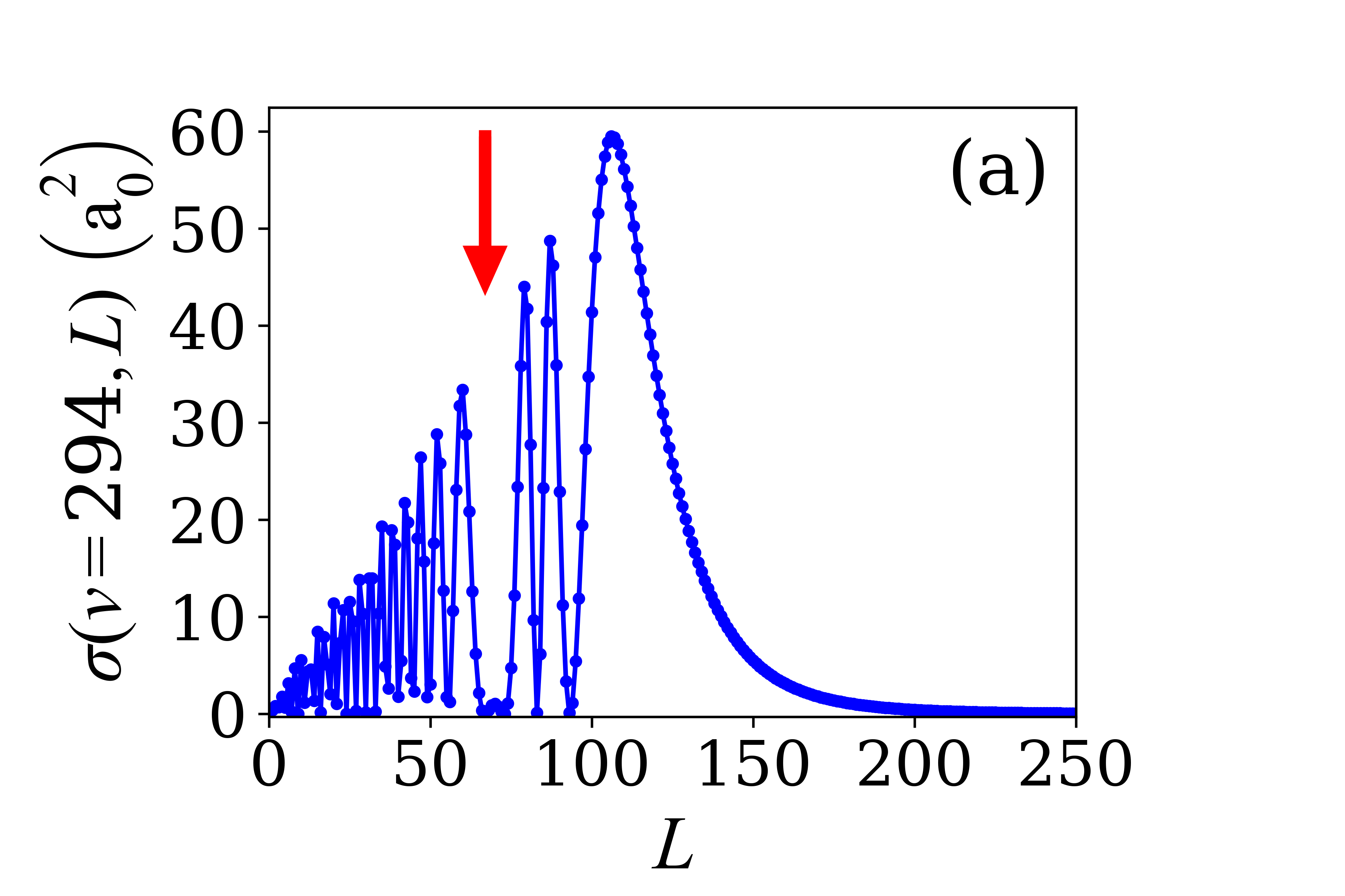
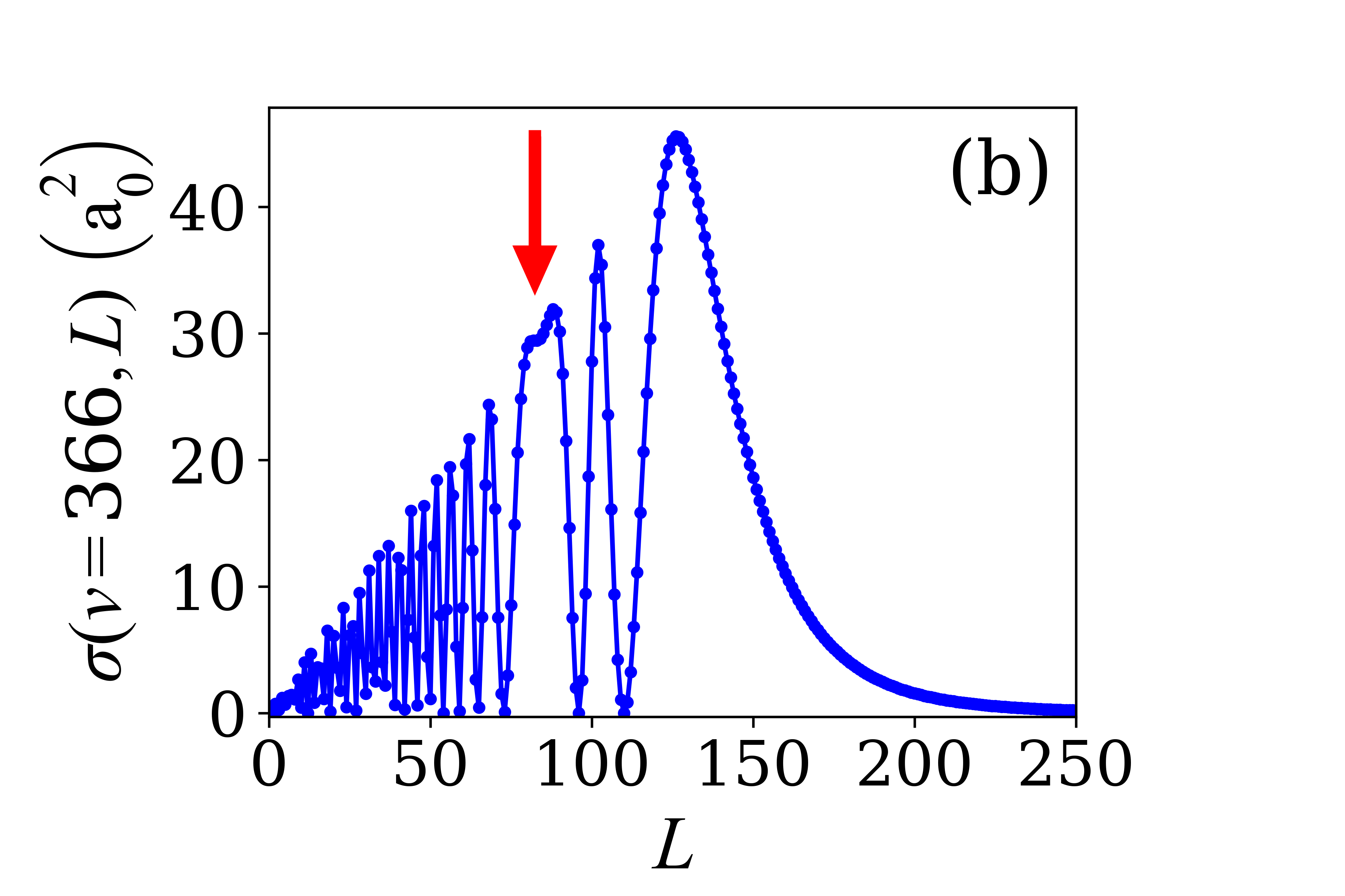
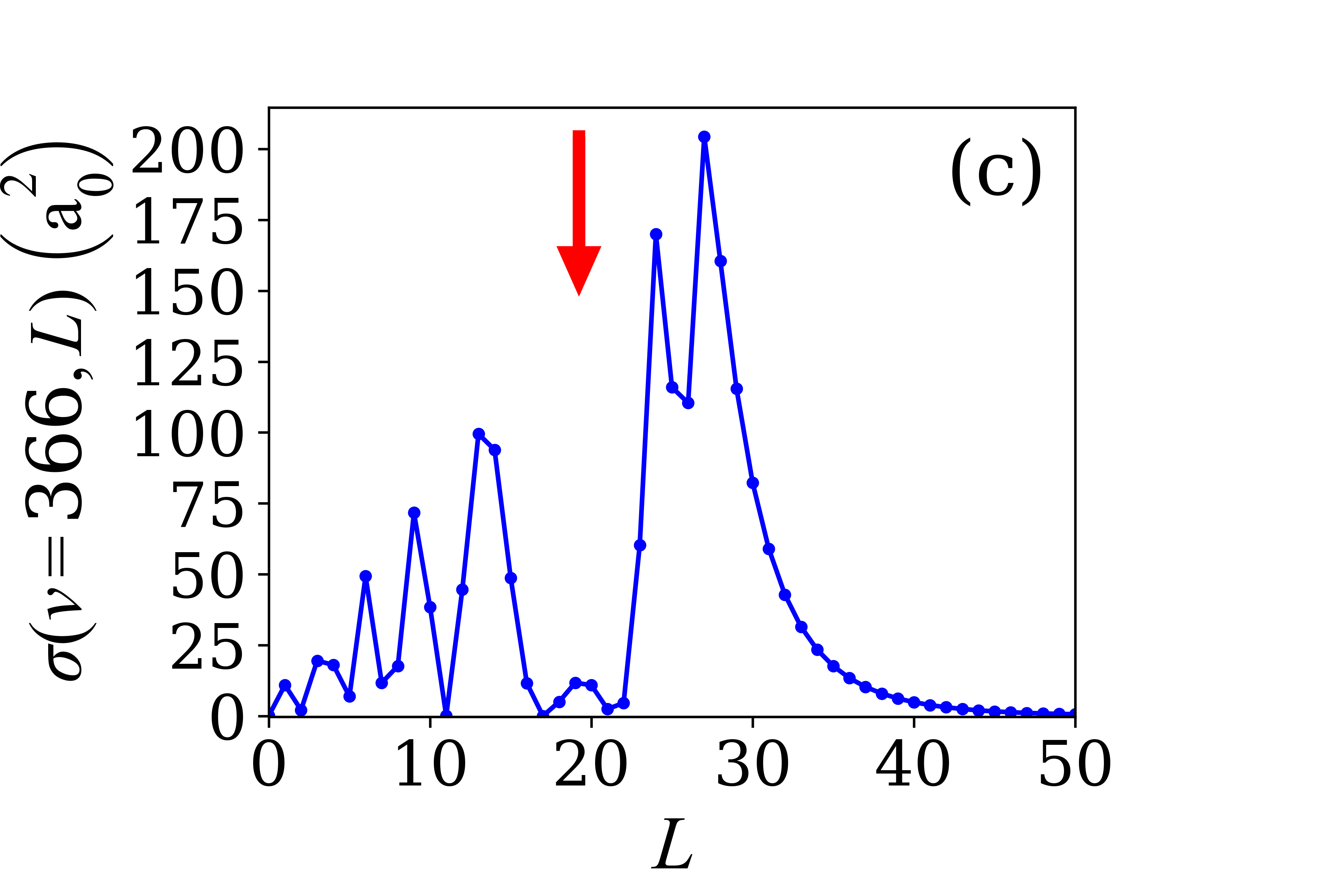
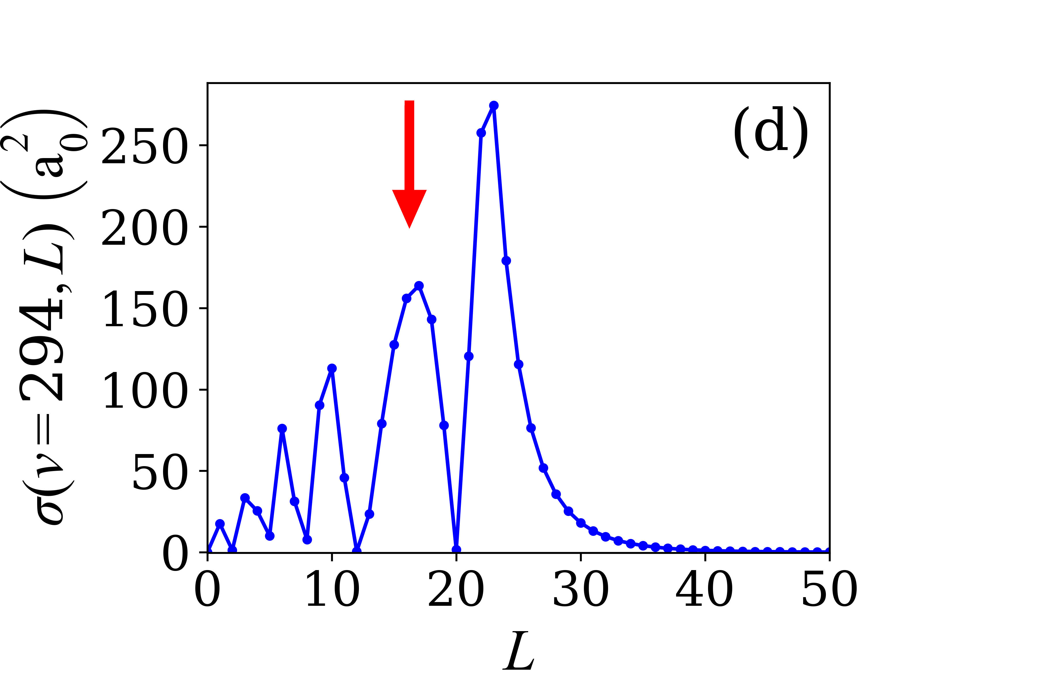
Figure 8: Illustrations of the effects of glory scattering interference: Plots of the $\sigma(v,L)$ versus $L$ at T = 294 K for ⁸⁷Rb-Ar using the LJ model (a) $v=294$ m/s, (b) $v=366$ m/s, and using the Klos Tiesinga (KT) potential [26] for ⁷Li-Ar (c) $v=366$ m/s and (d) $v=294$ m/s. The red arrow on each figure indicates the region near $L=L_{g}$ where variation of the scattering phase shifts in $L$ slows due to the short range contribution producing an interference minimum, as in (a) and (c), or a maximum, as in (b) and (d). This glory scattering interference changes from destructive to constructive as $v$ varies, leading to the undulations observed in Fig. 2.

A.2 The Long-Range Dominated Region, $v<v^{\rm{max}}_{C6}$

Once the values of $L_{g}$ have been estimated, their corresponding Jeffreys-Born (JB) phases, $\eta_{g}(v)$, can be deduced from Eq. 32,

$$\eta_{g}(v) = 0.15062\cdot\frac{\pi}{2}\cdot\left(\frac{v_{\rm{G}}}{v}\right)$$ (34)

where $v_{\rm{G}}$ is defined in Eq. 23 (refered to as $v^{*}$ in Child [30]). It is evident that this approximation will be valid for larger $v$ and fail as $v\rightarrow 0$.

Bernstein [33, 34] studied the $v$ dependence of the $\eta_{g}(v)$ values to predict the relative collision speeds where the maxima and minima of the glory undulations in $\sigma_{\rm{tot}}(v)$ occur. He reported the maxima occur when $\eta_{g}=(N-3/8)\pi$ and the minima at $\eta_{g}=(N-3/8+1/2)\pi$ where $N=1,2,3,\cdots$. The corresponding JB glory maxima will occur at velocities given by

$$v_{N}^{\rm{max}} = \frac{0.15062}{2\left(N-\frac{3}{8}\right)}v_{\rm{G}}.$$ (35)

The value for $N=1$ corresponds to the highest speed glory undulation maximum. This marks the upper relative collision speed limit where the long-range character of the potential dominates the $\sigma_{\rm{tot}}(v)$. We have labeled this value $v^{\rm{max}}_{C6}=v_{N=1}^{\rm{max}}$, Eq. 22, in the main body of this work. $v^{\rm{max}}_{C6}$ is a good estimate for the LJ potential since the JB approximation for the phase shifts is valid for large $v$. Indeed, the $v^{\rm{max}}_{C6}$ is also a good estimate for the location of the final maximum in $\sigma_{\rm{tot}}(v)$ for more realistic potentials such as those of references [26, 38]. Table 7 provides a comparison of the values for $R_{0}$, $v_{\rm{G}}$, $v^{\rm{max}}_{C6}$, and $N_{0}$ (the number of rotation-less bound states supported by the potential) for the Klos and Tiesinga (KT) published potentials [26] and the analytically derived values for a LJ potential with the same $C_{6}$ and potential depth, $D_{e}$. These values are compared for both ⁷Li-X and ⁸⁷Ar-X (X = H₂, He, Ne, N₂, Ar, Kr, and Xe) collisions. In particular we observe that $v^{\rm{max}}_{C6}$ values agree within 5% for the heavy background collision partners. Thus the LJ based value is a good estimate of the high speed glory maximum for the FQMS computation.

	$\mu$ (amu)	$R_{0}$ ($\rm{a_{0}}$)		$v_{\rm{p}}$ (m/s)	$v_{vdv}^{\rm{max}}$ (m/s)	$v_{\rm{G}}$ (m/s)		$v^{\rm{max}}_{C6}$ (m/s)			$N_{0}$
Collision Pair		12 LJ 12	12 KT 12			12 LJ 12	12KT 12	12 LJ 12	12 KT 12	KT:LJ	LJ	KT
87Rb-H2	1.97	9.73	10.22	1558	1908	3725	3912	449	472	1.05	2	2
87Rb-He	3.83	11.34	12.20	1105	1353	515	555	62	67	1.08	1	1
87Rb-Ne	16.38	9.59	10.04	492	603	2332	2441	281	294	1.05	3	4
87Rb-N2	21.18	9.67	10.07	418	512	9022	9396	1087	1132	1.04	8	8
87Rb-Ar	27.37	8.83	8.79	350	429	13593	13531	1638	1630	0.995	10	10
87Rb-Kr	42.66	8.59	8.29	242	296	23117	22998	2785	2687	0.965	16	16
87Rb-Xe	52.29	8.64	8.27	193	236	35216	33697	4243	4060	0.957	22	21
7Li-H2	1.57	8.37	8.58	1558	1908	4405	4516	531	544	1.03	1	1
7Li-He	2.55	9.52	10.14	1105	1353	627	667	76	80	1.06	1	1
7Li-Ne	5.21	8.30	8.67	492	603	2417	2524	291	304	1.04	2	2
7Li-N2	5.61	8.46	8.78	418	512	9248	9593	1114	1156	1.04	4	4
7Li-Ar	5.97	7.87	7.95	350	429	12523	12647	1509	1524	1.01	4	4
7Li-Kr	6.47	7.75	7.69	242	296	20270	20107	2442	2423	0.992	6	6
7Li-Xe	6.66	7.81	7.65	193	236	30796	30177	3711	3636	0.980	7	7

Table 7: A comparison of the $\mu$, $R_{0}$, $v_{\rm{G}}$, $v^{\rm{max}}_{C6}$ and $N_{0}$ values for the Klos and Tiesinga (KT) potential [26] and the analytically dervied values for a Lennard-Jones (LJ) potential with the same $C_{6}$ and $D_{e}$. Also included is the ratio of the KT:LJ $v^{\rm{max}}_{C6}$ (column 9) and the Maxwell-Boltzmann distribution peak speeds, $v_{\rm{p}}$, at T = 294K (column 4).

A.3 The number of glory undulations in $\sigma_{\rm{tot}}(v)$ vs $v$ : $N_{0}$

Bernstein [33, 34] and Child [30] assert that the number of glory undulations that appear in the $\sigma_{\rm{tot}}(v)$ versus $v$ spectrum is equal to the number of rotation-less bound states that can be supported by the potential, $N_{0}$. For a LJ potential this value is [34]

$$N_{0} = 0.27\sqrt{\frac{2\mu D_{e}R_{0}^{2}}{\hbar^{2}}}+\frac{1}{2}.$$ (36)

LJ potentials are completely defined by two parameters, $(C_{6},C_{12})$ or $(D_{e},R_{0})$, related by,

$$C_{6} = 4D_{e}R_{0}^{6}$$ (37)

$$C_{12} = 4D_{e}R_{0}^{12}.$$ (38)

Here it is convenient to define the LJ potentials with $C_{6}$ and $D_{e}$ which allows $N_{0}$ to be expressed as,

$$N_{0} = 0.27\sqrt{\frac{2\mu}{\hbar^{2}}}\left[\frac{C_{6}D_{e}^{2}}{4}\right]^{\frac{1}{6}}+\frac{1}{2}.$$ (39)

From this expression one observes the number of bound states depends on the reduced mass of the colliding partners, the depth of the potential, and on the $C_{6}$ value. Table 7 lists the values of $N_{0}$ determined using a LJ potential and using the KT potentials [26]. We observe that the they agree within 1 for the two types of potentials.

A.4 Estimate of the Relative Amplitude of Glory Undulations

We observe that the amplitude of the glory scattering induced undulation super-imposed on the underlying long-range character of the $\sigma_{\rm{tot}}(v)$ versus $v$ has the following properties (See Fig. 6).

1. The amplitude of the glory undulations is larger for lower reduced mass collision partners.

2. The amplitude of the glory undulations reduces as the relative collision speed increases for each collision pair.

Here we will provide an explanation for these two observations and estimate the undulation amplitude to demonstrate its dependence on the reduced mass, $\mu$, $C_{6}$, and $D_{e}$.

The effects of the interference generated by glory scattering is shown in Fig. 8: Each of the plots of $\sigma(v,L)$ vs $L$ share a similar character. From, Eq. 30 each partial wave contribution, $\sigma(v,L)$ has a $(2L+1)\sin^{2}\eta_{L}(v)$ dependence. The $\eta_{L}(v)$ phase shifts rise from a negative value (corresponding to the phase induced by the repulsive core [30]) through zero, reaching a positive peak at $L=L_{g}$, and then decreasing monotonically to zero as $L$ increases. Thus, the $\sigma(v,L)$ values oscillate for lower $L$ values and increase in amplitude with $L$. This oscillation ends in a final ”lobe” where $\sigma(v,L_{\pi})=0$ corresponding to $\eta_{L_{\pi}}(v)=\pi$ rising to the final peak appearing near $\eta_{L_{\pi/2}}(v)=\pi/2$, and then decreasing monotonically towards zero as $L\rightarrow\infty$ corresponding to $\eta_{L}(v)\rightarrow 0$. Using the Jeffreys-Born approximation for a purely $C_{6}$ long-range potential the position of $L_{\pi}$ is,

$$L_{\pi}(k) \approx \left[\left(\frac{3}{16}\right)\left(\frac{\mu C_{6}}{\hbar^{2}k}\right)\right]^{\frac{1}{5}}k$$

$$L_{\pi}(v) \approx \left[\left(\frac{3}{16}\right)\left(\frac{C_{6}}{\hbar}\right)\right]^{\frac{1}{5}}\cdot\left(\frac{\mu}{\hbar}\right)\cdot v^{\frac{4}{5}}.$$ (40)

This estimate indicates that the number of partial waves included in each $\sigma_{\rm{tot}}(v)$ increases as $\mu$, as $C_{6}^{\frac{1}{5}}$ and as $v^{\frac{4}{5}}$. Thus, one observes that the ⁸⁷Rb-Ar examples shown in Fig. 8 encompass many more partial waves than the corresponding ⁷Li-Ar values.

For $v<v^{\rm{max}}_{C6}$ these glory interference effects will occur with $L_{g}<L_{\pi}$. Thus, the glory-induced variation in the $\sigma(v)$ value can be approximated as the area of the slice of size $\Delta L$ centered on $L_{g}$,

$$\Delta\sigma_{g}(v) \approx \frac{2\pi}{k^{2}}L_{g}\cdot\Delta L$$ (41)

$$\approx \frac{2\pi}{k^{2}}\left[\frac{5\cdot 32}{11\cdot 21}\right]^{\frac{1}{5}}(kR_{0})\cdot\Delta L$$

$$\approx 2\pi\left[\frac{5\cdot 32}{11\cdot 21}\right]^{\frac{1}{5}}\left(\frac{\hbar}{\mu}\right)\cdot\left(\frac{C_{6}}{4D_{e}}\right)^{\frac{1}{6}}\cdot\frac{\Delta L}{v}$$

This value can be compared to the purely long-range $C_{6}$ estimate,

$$\sigma_{\rm{tot}}(v) \approx 8.0828\left(\frac{C_{6}}{\hbar v}\right)^{\frac{2}{5}}$$ (42)

to provide an estimate of the size of the relative glory undulation amplitude,

$$\frac{\Delta\sigma_{g}(v)}{\sigma_{\rm{tot}}(v)} \approx 0.722\left[\frac{\hbar}{C_{6}}\right]^{\frac{2}{5}}\left(\frac{\hbar}{\mu}\right)\frac{1}{v^{\frac{3}{5}}}\cdot R_{0}\cdot\Delta L$$ (43)

This estimate demonstrates that the glory undulation amplitude scales as $1/\mu$, leading to larger oscillations for lighter reduced mass. Assuming the $R_{0}$ and $\Delta L$ values are approximately equal for ⁷Li-Ar and ⁸⁷Rb-Ar, Eq. 43 predicts that the glory undulations in ⁷Li-Ar will be about 5 times larger than for ⁸⁷Rb-Ar.

Finally, the $v^{-\frac{3}{5}}$ dependence is consistent with the observation that the glory undulation amplitude decreases with increasing relative collision speed. (See Fig. 4(c), for example.)

Eq. 43 with v = $v_{\rm{p}}$ can be used to estimate the upper bound on the amplitude of the glory undulations to the underlying long-range (universal) prediction for $\left<\sigma_{\rm{tot}}\ v\right>$. That is, the ratio of $\Delta\sigma_{\rm{G}}(v_{\rm{p}})/\sigma_{\rm{tot}}(v)$ provides an estimate of the maximum relative residual effect of the glory oscillations on the total collision coefficients, $\left<\sigma_{\rm{tot}}\ v\right>$. In the absence of the velocity averaging minimization of the glory oscillations, this is the maximum glory scattering induced deviation from the long-range background cross-section one would expect. These values are shown on Fig. 9 and in Table 8. As expected, the lower the reduced mass of the collision partners, the larger the potential for the glory undulations to affect the value of $\left<\sigma_{\rm{tot}}\ v\right>$.

The actual residual effect of the glory undulations on the total collision rate coefficients, $\left<\sigma_{\rm{tot}}\ v\right>$, will depend on the number of undulations captured under the $v\cdot d(v)$ distribution used for the velocity averaging.

Figure 9: Plot of $\/\Delta\sigma_{\rm{G}}(v_{\rm{p}})/\sigma_{\rm{tot}}(v_{\rm{p}})$ (for T = 294K) versus $\mu$ using $v=v_{\rm{p}}$ as an estimate of the maximum residual effect of the glory undulations on the $\left<\sigma_{\rm{tot}}\ v\right>$ values. Here the ⁸⁷Rb-X and ⁷Li-X where X = N₂, Ar, Kr, and Xe are the species expected to be universal for which Eq. 43 is applicable. The ⁸⁷Rb-X are the red squares, while the violet squares are the ⁷Li-X values. Here $\Delta L=10$ was used for these estimates.

$\Delta\sigma_{\rm{G}}(v_{\rm{p}})/\sigma_{\rm{tot}}(v_{\rm{p}})$
Background	Sensor
Gas	87Rb	7Li
N2	0.029	0.123
Ar	0.024	0.122
Kr	0.016	0.117
Xe	0.012	0.109

Table 8: Estimates of the maximum relative deviation of the $\left<\sigma_{\rm{tot}}\ v\right>$ values from the $\left<\sigma_{\rm{tot}}\ v\right>_{\mathrm{SC}}$ due to the effects of glory undulations at T = 294K. The values are shown for ⁸⁷Rb-X (X = N₂, Ar, Kr, and Xe), column 2, and for ⁷Li-X (column 3). An estimate of $\Delta L=10$ was used for these computations.

Appendix B The Jeffreys-Born (JB) Approximation

Child [30] describes the Jeffreys-Born (JB) approximation for estimating the large $L$ elastic collision phase shifts, $\eta_{L}(k)$ in Chapter 4. This relies on the Born approximation for the wavefunctions describing the collision. Namely, the zero order approximation is

$$\psi^{0}_{L}(r) \approx krj_{L}(kr)$$ (44)

where $j_{L}(kr)$ is the Bessel function of order $L$. Using Green’s functions, Child then derives,

$$\eta_{L}(k) = -\frac{1}{k}\int_{0}^{\infty}\frac{2\mu V(r)}{\hbar^{2}}\left[\psi^{0}_{L}(r)\right]^{2}dr.$$ (45)

Different approximations for the expression for the wavefunctions, $\psi^{0}_{L}(r)$, lead to different approximations for $\eta_{L}(k)$.

B.1 The Jeffreys-Born Approximation, JB₀.

The initial approximation, JB₀, for the phase shifts, is to use the large $r$ asymptotic form for the Bessel functions to determine the phase shifts. Namely,

$$\left[\psi^{0}_{L}(r)\right]^{2} \approx k^{2}r^{2}j_{L}(kr)^{2}$$ (46)

$$\rightarrow \frac{1}{2\sqrt{1-\frac{L^{2}}{k^{2}r^{2}}}}.$$

Using Eq. 46 in Eq. 45, with $V(r)=-C_{6}/r^{6}$ one obtains,

$$\eta(k,L) \approx \frac{1}{k}\int_{0}^{\infty}\frac{2\mu C_{6}}{\hbar^{2}r^{6}}\left[\psi^{0}_{L}(r)\right]^{2}dr$$ (47)

$$\approx \frac{2\mu C_{6}}{\hbar^{2}k}\int_{L/k}^{\infty}\frac{dr}{2r^{6}\sqrt{1-\left(\frac{L}{kr}\right)^{2}}}$$

$$\approx \left(\frac{\mu C_{6}}{\hbar^{2}}\right)\frac{1}{k}\int_{L/k}^{\infty}\frac{dr}{r^{6}\frac{L}{kr}\sqrt{\left(\frac{kr}{L}\right)^{2}-1}}$$

$$\approx \left(\frac{\mu C_{6}}{\hbar^{2}}\right)\frac{k^{4}}{L^{5}}\int_{0}^{1}\frac{dz}{z^{5}\sqrt{z^{2}-1}}$$

where $z=kr/L$. This can be generalized for any $V(r)\leavevmode\nobreak\ =\leavevmode\nobreak\ C_{n}/r^{n}$,

$$\eta_{L}(k,C_{n},\rm{JB}_{0}) \approx -\left(\frac{\mu C_{n}}{\hbar^{2}}\right)\frac{k^{n-2}}{L^{n-1}}\int_{0}^{1}\frac{dz}{z^{n-1}\sqrt{z^{2}-1}}.$$ (48)

The integral over $z$ gives

$$\int_{0}^{1}\frac{dz}{z^{n-1}\sqrt{z^{2}-1}} = \sqrt{\pi}\frac{\Gamma\left(\frac{1}{2}\left(n-1\right)\right)}{\Gamma\left(\frac{n}{2}\right)}$$ (49)

providing the prefactor in front of each phase shift. This approximation has been used to deduce the values of $L_{g}$ and $L_{\pi}$ in Appendix A.

B.2 Refining the approximation, JB₁.

Child continues his discussion of the phase shifts by making the next approximation using the Bessel function form of the wavefunction in Eq. 45,

$$\eta_{L}(k) \approx -\frac{1}{k}\int_{0}^{\infty}\frac{2\mu V(r)}{\hbar^{2}}\left[k^{2}r^{2}j_{L}(kr)^{2}\right]dr.$$ (50)

Child [30] reports the result for a potential, $V(r)=C_{n}/r^{n}$, which is labeled JB₂ here,

$$\eta_{L}(k,C_{n},\rm{JB}_{2}) \approx -\frac{2\mu kC_{n}}{\hbar^{2}}\int_{0}^{infty}\frac{1}{r^{n-2}}j_{L}(kr)^{2}dr$$

$$= -\left(\frac{\pi}{2^{n-1}}\right)\left[\frac{(n-2)!}{(\frac{n}{2}!\cdot\frac{2}{n})^{2}}\right]\left(\frac{\mu C_{n}}{\hbar^{2}}\right)\cdot k^{n-2}\cdot q(L,n)$$

(51)

where,

$$q(L,n) = \frac{\Gamma(L+\frac{1}{2}-\frac{n}{2}+1)}{\Gamma(L+\frac{1}{2}-\frac{n}{2}+n)}.$$ (52)

Using the properties of Gamma functions, the ratio can be simplified, leaving an expression in the denominator which is the product of $n-1$ terms of the form $L+1/2-n/2+m$ where $m\in[n-1,n-2,...,1]$. The resulting polynomial has the leading term $L^{n-1}$. For large, $L$, only the leading term in the denominator is significant and $q(n,L)\rightarrow 1/L^{n-1}$ so that Eq. 51 reduces to the JB₀ estimate, Eq. 48.

Replacing $\ell=L+1/2$, one has,

$$q(L,n) = \frac{1}{\left(\ell-\frac{n}{2}+(n-1)\right)\left(\ell-\frac{n}{2}+(n-2)\right)\cdots\left(\ell-\frac{n}{2}+1\right)}$$

$$= \frac{1}{\ell^{n-1}\left(1+\frac{n-1+\frac{n}{2}}{\ell}\right)\left(1+\frac{n-2+\frac{n}{2}}{\ell}\right)\cdots\left(1+\frac{1+\frac{n}{2}}{\ell}\right)}.$$

Again, for large $\ell$, one has,

$$q(L,n,\rm{JB}_{1}) \approx \frac{1}{\ell^{n-1}}$$ (54)

and one obtains the JB₁ approximations applied in the main body of this paper,

$$\eta_{L}(k,C_{n},\rm{JB}_{1}) \approx -\left(\frac{\pi}{2^{n-1}}\right)\left[\frac{(n-2)!}{(\frac{n}{2}!\cdot\frac{2}{n})^{2}}\right]\left(\frac{\mu C_{n}}{\hbar^{2}}\right)\cdot\frac{k^{n-2}}{\ell^{n-1}}.$$

(55)

	FQMS $\left<\sigma_{\rm{tot}}\ v\right>$		$\left<\sigma_{\rm{tot}}\ v\right>_{\mathrm{KT}}$	$\left<\sigma_{\rm{tot}}\ v\right>_{\mathrm{SC}}$
	($10^{-15}$m3/s)		($10^{-15}$m3/s)	($10^{-15}$m3/s)
	KT[26]	Med[38]	K[26]	JB2	JB1	JB0
7Li-H2	3.114	—	3.173(60)	4.484	4.456	4.605
7Li-He	1.646	—	1.646(40)	2.313	2.308	2.378
7Li-Ne	1.557	—	1.558(140)	1.715	1.710	1.761
7Li-N2	2.597	—	2.634(20)	2.617	2.618	2.700
7Li-Ar	2.330	—	2.330(5)	2.303	2.311	2.345
7Li-Kr	2.141	—	2.141(4)	2.127	2.119	2.212
7Li-Xe	2.237	—	2.237(20)	2.210	2.205	2.308
87Rb-H2	3.927	—	3.887(99)	5.919	5.889	6.035
87Rb-He	2.369	2.443	2.370(30)	3.088	3.072	3.143
87Rb-Ne	2.039	1.983	1.996(200)	2.268	2.279	2.290
87Rb-N2	3.441	—	3.448(60)	3.453	3.452	3.481
87Rb-Ar	3.025	3.053	3.031(7)	3.012	2.999	3.023
87Rb-Kr	2.777	2.788	2.783(10)	2.774	2.771	2.782
87Rb-Xe	2.871	2.882	2.872(10)	2.881	2.876	2.874

Table 9: ⁷Li-X and ⁸⁷Rb-X (X = H₂, He, Ne, N₂, Ar, Kr, and Xe) $\left<\sigma_{\rm{tot}}\ v\right>$ values from the FQMS based on Kłos and Tiesinga (KT) potential [26], the Medvedev et al (Med) potential [38], the $K=K_{0}+K_{1}(T-300K)$ values from [26], and our SC computations $\left<\sigma_{\rm{tot}}\ v\right>_{\mathrm{SC}}$ using the different JB approximations for $\eta_{L}(k)$. The background gas ensemble temperature is 294 K.

For a purely attractive $C_{6}$ potential ($V(R)=-C_{6}/r^{6}$), the $\left<\sigma_{\rm{tot}}v\right>_{\rm{C6}}$ corresponding to JB₀ and JB₁ can be written analytically:

$$\left<\sigma_{\rm{tot}}v\right>_{\rm{C6}}^{JB_{0}} \approx 8.49463\left(\frac{C_{6}}{\hbar v_{\rm{p}}}\right)^{\frac{2}{5}}v_{\rm{p}}+7.19729\left(\frac{\hbar}{\mu}\right)\left(\frac{C_{6}}{\hbar v_{\rm{p}}}\right)^{\frac{1}{5}}$$

and

$$\left<\sigma_{\rm{tot}}v\right>_{\rm{C6}}^{JB_{1}} \approx 8.49463\left(\frac{C_{6}}{\hbar v_{\rm{p}}}\right)^{\frac{2}{5}}v_{\rm{p}}.$$ (57)

One notes the JB₀ approximation contains an extra term in $\hbar/\mu$. The JB₂ approximation for $\eta_{L}(k)$ (Eq. 51) does not yield a simple analytical expression but can be used to compute $\left<\sigma_{\rm{tot}}v\right>_{\rm{C6}}^{JB_{2}}$.

To evaluate the differences between the approximations, JB₀, JB₁, and JB₂, the $\left<\sigma_{\rm{tot}}\ v\right>_{\mathrm{SC}}$ were computed using the three approximations for $\eta_{L}(k)$. These were compared to FQMS computations based on the Kłos and Tiesinga (KT) [26] and Medvedev et al (Med) [38] potentials, and to the values of $K=K_{0}+(T-300K)$ reported by Klos and Tiesinga [26]. (See Table 9.) The background gas temperature used in these computations was 294 K.

In addition, Table 10 contains the $\left<\sigma_{\rm{tot}}v\right>_{\rm{C6}}$ values computed based on the analytical JB₀ approximation (a-JB₀), Eq. LABEL:eqB:svtotC6JB0, the analytical JB₁ approximation (a-JB₁), Eq. 57, and the numerically computed $\left<\sigma_{\rm{tot}}v\right>_{\rm{C6}}$ values, JB₀, JB₂, and JB₁.

	$\left<\sigma_{\rm{tot}}v\right>_{\rm{C6}}$
	($10^{-15}$m3/s)
	a-JB0	a-JB1	JB0	JB1	JB2
7Li-H2	4.094	3.935	4.092	3.935	3.948
7Li-He	1.981	1.901	1.980	1.898	1.906
7Li-Ne	1.579	1.526	1.575	1.523	1.523
7Li-N2	2.526	2.458	2.537	2.467	2.452
7Li-Ar	2.223	2.157	2.219	2.168	2.157
7Li-Kr	2.100	2.030	2.111	2.039	2.036
7Li-Xe	2.208	2.130	2.246	2.137	2.143
87Rb-H2	5.118	4.976	5.112	4.972	4.995
87Rb-He	2.552	2.490	2.553	2.488	2.493
87Rb-Ne	2.026	2.007	2.026	2.004	2.007
87Rb-N2	3.198	3.177	3.195	3.181	3.180
87Rb-Ar	2.823	2.807	2.819	2.816	2.813
87Rb-Kr	2.641	2.628	2.638	2.631	2.628
87Rb-Xe	2.763	2.752	2.770	2.752	2.751

Table 10: The $\left<\sigma_{\rm{tot}}v\right>_{\rm{C6}}$ values of ⁷Li-X and ⁸⁷Rb-X $\left<\sigma_{\rm{tot}}v\right>_{\rm{C6}}$ for X = (H₂, He, Ne, N₂, Ar, Kr, and Xe) based on the analytical JB₀ (a-JB₀) expression, Eq. LABEL:eqB:svtotC6JB0, the analytical expressions JB₁ (a-JB₁), Eq. 57, and substantiated by numerical computations for the JB₀, JB₁, and JB₂ approximations of the phase shifts $\eta_{L}(k)$. Here T = 294 K.

Examining the results of these computations:

• The $\left<\sigma_{\rm{tot}}\ v\right>_{\mathrm{SC}}$ values for the JB₂ and JB₁ approximations are in good agreement with each other and with the FQMS $\left<\sigma_{\rm{tot}}\ v\right>$ computations based on the KT and Medvedev potentials for the universal species ⁷Li-X and ⁸⁷Rb-X, where X = (N₂, Ar, Kr, and Xe).

• The $\left<\sigma_{\rm{tot}}\ v\right>_{\mathrm{SC}}$ from JB₀ is systematically a larger than the other values for both ⁷Li-X and ⁸⁷Rb-X in all cases, X = H₂, He, Ne, N₂, Ar, Kr, excepting ⁸⁷Rb-Xe.

Thus, the $\left<\sigma_{\rm{tot}}\ v\right>_{\mathrm{SC}}$ JB₁ values are a good heuristic to compare the universal species’ $\left<\sigma_{\rm{tot}}\ v\right>$ values against.

Next the $\left<\sigma_{\rm{tot}}v\right>_{\rm{C6}}$ results:

• There is consistency between the analytical expressions and their corresponding numerical computations of $\left<\sigma_{\rm{tot}}v\right>_{\rm{C6}}$ (a-JB₀ = JB₀, and a-JB₁ = JB₁).

• The JB₀ estimates for $\left<\sigma_{\rm{tot}}v\right>_{\rm{C6}}$ are systematically larger than the corresponding JB₁ and the JB₂ estimates, as one would expect since the JB₀ has the extra small $\hbar/\mu$ term in Eq. LABEL:eqB:svtotC6JB0.

• The $\left<\sigma_{\rm{tot}}v\right>_{\rm{C6}}$ JB₁ and JB₂ values agree well with each other.

Thus, the $\eta_{L}(k,\rm{JB}_{1})$ (Eq. 51) are used for computing the $\left<\sigma_{\rm{tot}}\ v\right>_{\mathrm{SC}}$ and $\left<\sigma_{\rm{tot}}v\right>_{\rm{C6}}$ in the main body of this paper.

References

- Booth et al. [2011] J. Booth, D. E. Fagnan, B. G. Klappauf, K. W. Madison, and J. Wang, Method and device for accurately measuring the incident flux of amibient particles in a high or ultra-high vacuum environment (2011), uS Patent 8,803,072.
- Madison [2012] K. W. Madison, A cold atom based pressure standard, personal communication (2012), seminar at the National Institute of Standards and Technology, Gaithersburg, MD, December 4, 2012; seminar at the Laboratoire national de métrologie et d’essais, Paris, FRANCE, March 26, 2013.
- Arpornthip et al. [2012] T. Arpornthip, C. A. Sackett, and K. J. Hughes, Vacuum-pressure measurement using a magneto-optical trap, Phys. Rev. A 85, 033420 (2012).
- Yuan et al. [2013] J.-P. Yuan, Z.-H. Ji, Y.-T. Zhao, X.-F. Chang, L.-T. Xiao, and S.-T. Jia, Simple, reliable, and nondestructive method for the measurement of vacuum pressure without specialized equipment, Appl. Opt. 52, 6195 (2013).
- Moore et al. [2015] R. W. G. Moore, L. A. Lee, E. A. Findlay, L. Torralbo-Campo, G. D. Bruce, and D. Cassettari, Measurement of vacuum pressure with a magneto-optical trap: A pressure-rise method, Review of Scientific Instruments 86, 093108 (2015), https://doi.org/10.1063/1.4928154 .
- Makhalov et al. [2016] V. B. Makhalov, K. A. Martiyanov, and A. V. Turlapov, Primary vacuometer based on an ultracold gas in a shallow optical dipole trap, Metrologia 53, 1287 (2016).
- Makhalov and Turlapov [2017] V. B. Makhalov and A. V. Turlapov, A vacuum gauge based on an ultracold gas, Quantum Electronics 47, 431 (2017).
- Scherschligt et al. [2017] J. Scherschligt, J. A. Fedchak, D. S. Barker, S. Eckel, N. Klimov, C. Makrides, and E. Tiesinga, Development of a new uhv/xhv pressure standard (cold atom vacuum standard), Metrologia 54, S125 (2017).
- Scherschligt et al. [2018] J. Scherschligt, J. A. Fedchak, Z. Ahmed, D. S. Barker, K. Douglass, S. Eckel, E. Hanson, J. Hendricks, N. Klimov, T. Purdy, J. Ricker, R. Singh, and J. Stone, Review article: Quantum-based vacuum metrology at the national institute of standards and technology, Journal of Vacuum Science & Technology A 36, 040801 (2018).
- Eckel et al. [2018] S. Eckel, D. S. Barker, J. A. Fedchak, N. N. Klimov, E. Norrgard, J. Scherschligt, C. Makrides, and E. Tiesinga, Challenges to miniaturizing cold atom technology for deployable vacuum metrology, Metrologia 55, S182 (2018).
- Xiang et al. [2018] J.-f. Xiang, H.-n. Cheng, X.-k. Peng, X.-w. Wang, W. Ren, J.-w. Ji, K.-k. Liu, J.-b. Zhao, L. Li, Q.-z. Qu, T. Li, B. Wang, M.-f. Ye, X. Zhao, Y.-y. Yao, D.-S. Lü, and L. Liu, Loss of cold atoms due to collisions with residual gases in free flight and in a magneto-optical trap, Chinese Physics B 27, 073701 (2018).
- Booth et al. [2019] J. L. Booth, P. Shen, R. V. Krems, and K. W. Madison, Universality of quantum diffractive collisions and the quantum pressure standard, New Journal of Physics 21, 102001 (2019).
- Shen et al. [2020] P. Shen, K. W. Madison, and J. L. Booth, Realization of a universal quantum pressure standard, Metrologia 57, 025015 (2020).
- Shen et al. [2021] P. Shen, K. W. Madison, and J. L. Booth, Refining the cold atom pressure standard, Metrologia 58, 022101 (2021).
- Barker et al. [2021] D. Barker, N. Klimov, E. Tiesinga, J. Fedchak, J. Scherschligt, and S. Eckel, Progress towards comparison of quantum and classical vacuum standards, Measurement: Sensors 18, 100229 (2021).
- Ehinger et al. [2022a] L. H. Ehinger, B. P. Acharya, D. S. Barker, J. A. Fedchak, J. Scherschligt, E. Tiesinga, and S. Eckel, Comparison of two multiplexed portable cold-atom vacuum standards, AVS Quantum Science 4, 034403 (2022a).
- Zhang et al. [2022] S.-Z. Zhang, W.-J. Sun, M. Dong, H.-B. Wu, R. Li, X.-J. Zhang, J.-Y. Zhang, and Y.-J. Cheng, Vacuum pressure measurement based on 6li cold atoms in a magneto-optical trap, Acta Phys. Sin. 71, 094204 (2022).
- Ehinger et al. [2022b] L. H. Ehinger, B. P. Acharya, D. S. Barker, J. A. Fedchak, J. Scherschligt, E. Tiesinga, and S. Eckel, Comparison of two multiplexed portable cold-atom vacuum standards, AVS Quantum Science 4, 034403 (2022b).
- Sun et al. [2024] W. Sun, X. Wu, Y. Cheng, M. Dong, Z. Ma, W. Jia, Y. Zhang, R. Zhang, C. Wu, C. Feng, and H. Luo, Cold atom technology applied to ultra-high vacuum (uhv) measurements, Vacuum 222, 113079 (2024).
- Barker et al. [2023] D. S. Barker, J. A. Fedchak, J. Kłos, J. Scherschligt, A. A. Sheikh, E. Tiesinga, and S. P. Eckel, Accurate measurement of the loss rate of cold atoms due to background gas collisions for the quantum-based cold atom vacuum standard, AVS Quantum Science 5, 035001 (2023).
- Eckel et al. [2023] S. Eckel et al., in preparation (2023).
- Makrides et al. [2019] C. Makrides, D. S. Barker, J. A. Fedchak, J. Scherschligt, S. Eckel, and E. Tiesinga, Elastic rate coefficients for collisions in the calibration of a cold-atom vacuum standard, Phys. Rev. A 99, 042704 (2019).
- Makrides et al. [2020] C. Makrides, D. S. Barker, J. A. Fedchak, J. Scherschligt, S. Eckel, and E. Tiesinga, Collisions of room-temperature helium with ultracold lithium and the van der waals bound state of heli, Phys. Rev. A 101, 012702 (2020).
- Makrides et al. [2022a] C. Makrides, D. S. Barker, J. A. Fedchak, J. Scherschligt, S. Eckel, and E. Tiesinga, Erratum: Collisions of room-temperature helium with ultracold lithium and the van der waals bound state of heli [phys. rev. a 101, 012702 (2020)], Phys. Rev. A 105, 029902 (2022a).
- Makrides et al. [2022b] C. Makrides, D. S. Barker, J. A. Fedchak, J. Scherschligt, S. Eckel, and E. Tiesinga, Erratum: Elastic rate coefficients for collisions in the calibration of a cold-atom vacuum standard [phys. rev. a 99, 042704 (2019)], Phys. Rev. A 105, 039903 (2022b).
- Kłos and Tiesinga [2023] J. Kłos and E. Tiesinga, Elastic and glancing-angle rate coefficients for heating of ultracold li and rb atoms by collisions with room-temperature noble gases, h2 , and n2, The Journal of Chemical Physics 158, 014308 (2023).
- Madison et al. [2018] K. Madison, J. Booth, P. Shen, and R. Krems, Quantum pressure standard and methods for determining and using same (2018), uS Patent US11221268B2.
- Stewart et al. [2022] R. A. Stewart, P. Shen, J. L. Booth, and K. W. Madison, Measurement of rb-rb van der waals coefficient via quantum diffractive universality, Phys. Rev. A 106, 052812 (2022).
- Shen et al. [2023] P. Shen, E. Frieling, K. R. Herperger, D. Uhland, R. A. Stewart, A. Deshmukh, R. V. Krems, J. L. Booth, and K. W. Madison, Cross-calibration of atomic pressure sensors and deviation from quantum diffractive collision universality for light particles, New Journal of Physics 25, 053018 (2023).
- Child [1996] M. Child, Molecular Collision Theory, Dover Books on Chemistry Series (Dover Publications, 1996).
- Deshmukh et al. [2024] A. Deshmukh, R. A. Stewart, P. Shen, J. L. Booth, and K. W. Madison, Trapped-particle evolution driven by residual gas collisions, Phys. Rev. A 109, 032818 (2024).
- Bali et al. [1999] S. Bali, K. M. O’Hara, M. E. Gehm, S. R. Granade, and J. E. Thomas, Quantum-diffractive background gas collisions in atom-trap heating and loss, Phys. Rev. A 60, R29 (1999).
- Bernstein [1962] R. B. Bernstein, Extrema in Velocity Dependence of Total Elastic Cross Sections for Atomic Beam Scattering: Relation to Di‐atom Bound States, The Journal of Chemical Physics 37, 1880 (1962), https://pubs.aip.org/aip/jcp/article-pdf/37/8/1880/18827611/1880_1_online.pdf .
- Bernstein [1963] R. B. Bernstein, Semiclassical Analysis of the Extrema in the Velocity Dependence of Total Elastic‐Scattering Cross Sections: Relation to the Bound States, The Journal of Chemical Physics 38, 2599 (1963), https://pubs.aip.org/aip/jcp/article-pdf/38/11/2599/18829522/2599_1_online.pdf .
- Loesch and Stienkemeier [1993] H. J. Loesch and F. Stienkemeier, Evidence for the deep potential well of Li+HF from backward glory scattering, The Journal of Chemical Physics 99, 9598 (1993), https://pubs.aip.org/aip/jcp/article-pdf/99/12/9598/19078426/9598_1_online.pdf .
- Besemer et al. [2022] M. Besemer, G. Tang, Z. Gao, A. Avoird, G. Groenenboom, S. Meerakker, and T. Karman, Glory scattering in deeply inelastic molecular collisions, Nature Chemistry 14 (2022).
- Roberts et al. [2002] T. D. Roberts, A. D. Cronin, D. A. Kokorowski, and D. E. Pritchard, Glory oscillations in the index of refraction for matter waves, Phys. Rev. Lett. 89, 200406 (2002).
- Medvedev et al. [2018] A. A. Medvedev, V. V. Meshkov, A. V. Stolyarov, and M. C. Heaven, Ab initio interatomic potentials and transport properties of alkali metal (m = rb and cs)–rare gas (rg = he, ne, ar, kr, and xe) media, Phys. Chem. Chem. Phys. 20, 25974 (2018).
- Jiang et al. [2015] J. Jiang, J. Mitroy, Y. Cheng, and M. Bromley, Effective oscillator strength distributions of spherically symmetric atoms for calculating polarizabilities and long-range atom–atom interactions, Atomic Data and Nuclear Data Tables 101, 158 (2015).