Bayesian Deep ICE

Abstract

Deep Independent Component Estimation (DICE) has many applications in modern day machine learning as a feature engineering extraction method. We provide a novel latent variable representation of independent component analysis that enables both point estimates via expectation-maximization (EM) and full posterior sampling via Markov Chain Monte Carlo (MCMC) algorithms. Our methodology also applies to flow-based methods for nonlinear feature extraction. We discuss how to implement conditional posteriors and envelope-based methods for optimization. Through this representation hierarchy, we unify a number of hitherto disjoint estimation procedures. We illustrate our methodology and algorithms on a numerical example. Finally, we conclude with directions for future research.

Key words: Deep Learning, ICE, factor models, Bayes, Flow models.

1 Introduction

Linear independent component analysis (ICA) is central to blind source separation and has many fields of application. Our work builds on the seminal work of MacKay, (1992) who interprets ICA as a latent variable modeling strategy. With this interpretation, MacKay, (1992) shows that the original blind separation algorithm of Bell and Sejnowski, (1995) can be viewed as a MAP estimator from the marginalised likelihood. The latent variable model with a separable distribution on the hidden states.

Feature engineering (a.k.a. nonlinear factor analysis) is a fundamental problem in many modern day machine learning applications ranging from medical imaging to signal processing. A key aspect of feature engineering is decomposing high-dimensional data into independent latent factors. Linear independent components analysis (ICA) separates the observed data into a lower-dimensional array of independent sources (a.k.a. features) to offer a high-dimensional probabilistic structure. Such tools fall into the class of high-dimensional data reduction methods and help one identify pivotal data features as well as yield optimal predictive outcomes. A key feature of popular statistical or ML models is that they necessitate an approach that concurrently discerns both the foundational independent features and their associated mixing weights, colloquially termed as nonlinear mixing maps.

Our primary objective is to unify an array of algorithmic approaches to allow for both a fully Bayesian and MAP optimization. Method of moments estimators are also commonplace in this literature. We build on the seminal work of (MacKay,, 1992, 1996) who showed that the (Bell and Sejnowski,, 1995) algorithm for signal processing for a non-linear feedforward network can be viewed as a maximum likelihood algorithm for the optimisationn of a linear generative model. Our contribution then is three-fold:

1. Develop full Bayesian methods for ICA

2. Unify existing models using scale mixtures of normals

3. Develop Nonlinear deep ICE

Blind source separation is a classical problem in signal processing. In the formulation by (Herault and Jutten,, 1986; Bell and Sejnowski,, 1995), algorithms for blind source separation attempt to recover source signals ${\bf s}$ from observations ${\bf x}$, where ${\bf x}={\bf V}{\bf s}$, are linear mixtures with unknown weights ${\bf V}$. This is done by finding a square matrix ${\bf W}$ which is the inverse of the mixing matrix ${\bf V}$, up to permutation and change of scale. For example, (Bell and Sejnowski,, 1994, 1995) take an algorithmic approach summarised as a linear mapping ${\bf a}={\bf W}{\bf x}$ where $\mathbf{a}$ is an estimate of the source signals. This is done by adjusting the unmixing matrix ${\bf W}$ to maximize the entropy of the outputs. The algorithm proceeds iteratively using a gradient ascent method on the log-likelihood of the estimated sources, where the update rule for $W$ is:

$$\nabla W\propto\left(I-2\phi(\mathbf{a})\mathbf{a}^{T}\right){\bf W}$$

where, $I$ is the identity matrix, and $\phi(\mathbf{a})$ is a non-linear function applied component-wise to $\mathbf{a}$. Common choices for $f$ are the logistic sigmoid function or the hyperbolic tangent (i.e., a nonlinear map ${\bf z}_{i}=\phi_{i}({\bf a}_{i})$ where $\phi=-\tanh$.

Our work takes a Bayesian approach with an assumption as a source distribution, ${\bf s}\sim p({\bf s})$. This distribution acts as a regularization penalty and allows us to unify existing procedures as MAP estimators. For example, MacKay, (1996) shows that if $\phi_{i}(a_{i})=-\tanh(a_{i})$ then this is equivalent to a source distribution of the form $p_{i}(s_{i})\propto 1/\cosh(s_{i})=1/(e^{s_{i}}+e^{-s_{i}})$. We argue in §2 that this can be written as a scale mixture of Normals using a Pólya-Gamma mixing density. Moreover, MacKay suggests adding a gain $\beta$ and considering a heavy-tailed source distribution of the form $p_{i}(s_{i})\propto 1/\cosh^{1/\beta}(\beta s_{i})$. Again we show that this can be represented as a Normal scale mixture thus leading to classes of auxiliary variable methods for inference and optimisation. In the limit as $\beta\to\infty$ this becomes $p_{i}(s_{i})\propto\exp(-\lvert s_{i}\rvert)$ the double exponential (a.k.a. Lasso) prior, and as $\beta\to 0$, $p_{i}(s_{i})$ would converge to a zero-mean Gaussian with variance $1/\beta$.

The Bayesian approach (Févotte et al.,, 2004; Févotte and Godsill,, 2006; Donnat et al.,, 2019; MacKay,, 1992) has a two-fold advantage. First, rather than casting problem as a method of moments approach (kurtosis), a Bayesian approach finds the solution by a suitable regularization with a heavy-tailed prior (thus imposing constraint on higher order moments). A particular suitable class is super-Gaussian priors (Palmer et al.,, 2006) via scale mixtures of normals (West,, 1987). MacKay, (1992) uses a heavy-tailed source distribution towards this. The advantage is that mixture and envelope methods can be used to extract features/factors and provide fast scalable algorithms for ICA. In this paper, we unify the existing Bayesian algorithms and provide new ones.

A related goal is to bring together the modeling of source distributions under the encompassing paradigm of Gaussian scale mixtures (Andrews and Mallows,, 1974; West,, 1987; Carlin and Polson,, 1991). This latent variable or parameter expansion approach offers fast, scalable algorithms akin to the auxiliary variable methods proposed by (Ono and Miyabe,, 2010). Furthermore, it obviates dependence on approximative techniques like variational Bayes (VB). Our methodology bears significance for deep Bayesian models wherein latent variable distributions are forged as superpositions of nonlinear mappings, akin to deep learning constructs (Polson and Sokolov,, 2017).

On the algorithmic side, we show that a number of hitherto disjoint algorithms can be unified as envelope optimisation methods, see Geman and Yang, (1995) and (Polson and Scott,, 2016). For example, the ICA updating scheme due to Bell and Sejnowski, (1995) is equivalent to a maximum likelihood approach, see (MacKay,, 1992, 1996). Auxiliary variable methods allow for both EM and MCMC algorithms to be developed across a wide spectrum of source distributions. Such methods can lead to faster convergence (Ono and Miyabe,, 2010) and can incorporate methods for fast convergence such as Nesterov acceleration and block-coordinate descent, thus providing an alternative to traditional stochastic gradient descent methods.

The hallmark of ICA methods is the use of a super-Gaussian distribution over hidden states. Surprisingly, this leads to identification where traditional Gaussian modeling assumptions do not. A linear mixing of Gaussian distribution is itself Gaussian, so de-mixing is impossible. Hence the source distribution must have heavy tails (a.k.a. super-Gaussian) and the easiest way to achieve this is via scale mixtures of normals (West,, 1987; Barndorff-Nielsen et al.,, 1982). The key insight then that underlies our unifying approach is that the components of the source distribution can be modeled with scale mixtures of normals. We show that MacKay’s original model and its extensions are simply scale mixtures with Pólya-Gamma mixing (Polson et al.,, 2013).

The rest of our paper is outlined as follows. The next subsection describes connections with previous work. Section 2 provides a discussion of deep Bayesian generative models. Section 3 provides a unifying framework for super-Gaussian source distributions. Section 4 discusses envelope methods to provide fast optimisation methods. Section 5.1 illustrates our methodology. Finally, Section 6 concludes with directions for future research.

1.1 Connections with Previous Work

Samworth and Yuan, (2012) proposes a nonparametric maximum likelihood approach for estimating the unmixing weights and the marginal distributions by projecting the empirical distributions on the space of log-concave univariate distributions. They also address the question of identifiability of the unmixing matrices, first studied by (Comon,, 1994), and in their formulation identifiability up to scaling and permutation is guaranteed by requiring that not more than one of the univariate log-concave projections is Gaussian. This is also connected to Kruskal’s identifiability conditions (Kruskal,, 1977) for a tensor product $T=\sum_{r=1}^{R}A\otimes B\otimes C$, in terms of the Kruskal ranks of the individual matrices: $\kappa_{A}+\kappa_{B}+\kappa_{C}\geq 2R+2$. Bhaskara et al., (2014) provide a robust version of the identifiability theorem for approximate recovery and point uses in several latent variable models.

Camuto et al., (2021) combine a linearly independent component analysis (ICA) with nonlinear bisective feature maps (from flow-based methods). For non-square ICA, they can assume the number of sources is less than the data dimensionality – thus achieving better unsupervised latent factor discovering than other ICA flow-based methods. Dinh et al., (2014) discuss NICE deep generative models with nonlinear invertible neural networks, building on the work of Deco and Obradovic, (1996), Obradovic and Deco, (1998), Comon et al., (1991) and Pearlmutter and Parra, (1996) and Malthouse, (1998). Recent work includes Bayesian ICA models of (Donnat et al.,, 2019). Other related approaches include auto-encoder and sparsity models.

Nonlinear ICA models have been proposed by Hyvärinen and Pajunen, (1999), although identification can be challenging. Khemakhem et al., (2020) provides recent identification results, providing mild conditions under which the joint distribution encompassing both observed and latent variables within Variational Autoencoders (VAEs) are identifiable and estimable, thus establishing a connection between VAEs and nonlinear Independent Component Analysis (ICA).

The source ${\bf s}$ is a feature vector that needs to be learned, see, for example, Olshausen and Field, (1996, 1997) for sparse coding of natural images, where an image is modeled as a natural superposition using an over-complete basis set where the amplitudes are given sparsity-inducing prior distributions. This is based on the intuition of Barlow’s principle of redundancy reduction (Barlow,, 1989, 2001).

Other popular approaches for dimension reduction include Sliced Inverse Regression (Li,, 1991) that finds a low-dimensional projection of the data that captures the most relevant information for explaining the variation in the data, specifically designed for non-linear relationships in the data, Unlike traditional linear dimensionality reduction methods like Principal Component Analysis (PCA). Lopes et al., (2012) introduces a sequential online strategy for efficient posterior simulation. Finally, as noted by Brillinger, (2012) and Naik and Tsai, (2000), the mixing matrix can be consistently estimated through PLS, regardless of the activation function’s nonlinearity, albeit with a proportionality constant. While the assumption by Brillinger, (2012) of Gaussian input ${\bf X}$ is necessary for applying Stein’s lemma, we note that this outcome extends to scale-mixtures of Gaussians.

NICE (non-linear independent component estimation)

Dinh et al., (2014) provide a deep learning framework called the for high-dimensional density estimation, followed by the real NVP (Dinh et al.,, 2016) transformations for unsupervised learning. The real NVP method learns a stable and invertible bijective function or map between samples $x\sim p_{X}$ and latent space $s\sim p_{S}$ or, $\theta\sim p_{\theta}$. For example, Trippe and Turner, (2018) utilize normalizing flows as likelihoods for conditional density estimation for complex densities. Jimenez Rezende and Mohamed, (2015) provide an approximation framework using a series of parametric transformations for complex posteriors. A new method for Monte Carlo integration called Neural Importance Sampler was provided by Müller et al., (2019) based on the NICE framework by parametrizing the proposal density by a collection of neural networks.

Invertible Neural Network: An important concept in the context of generative models is an invertible neural network or INNs (Dinh et al.,, 2016). Loosely speaking, an INN is a one-to-one function with a forward mapping $f:\mathbb{R}^{d}\mapsto\mathbb{R}^{d}$, and its inverse $g=f^{-1}$. Song et al., (2019) provides the ‘MintNet’ algorithm to construct INNs by using simple building blocks of triangular matrices, leading to efficient and exact Jacobian calculation. On the other hand, Behrmann et al., (2021) show that common INN method suffer from exploding inverses and provide conditions for stability of INNs. For image representation, Jacobsen et al., (2018) introduce a deep invertible network, called the i-revnet, that retains all information from input data up until the final layer.

Flow transformation models:

Here ${\bf y}=h({\bf x})$ where $h(\cdot)$ is typically modeled as an invertible neural network (INN), with both $p_{y}$ and $p_{F}$ as Gaussian densities,

$$p({\bf y},{\bf x}\mid{\bf s}) =p({\bf y}|{\bf x},{\bf s})p({\bf x}|{\bf s})$$

$$=p_{y}({\bf y}\mid h^{-1}({\bf x}),{\bf s})p_{F}(h^{-1}({\bf x}))\left|\frac{\partial h^{-1}}{\partial{\bf x}}\right|$$

where the determinant of Jacobian is easy to compute. These models can be thought of as latent factor models. Flow-based methods have been used to construct a nonlinear ICA where the dimensionality of the latent space is equal to the data as in an auto-encoder approach, see Camuto et al., (2021).

Latent Factor Model: Another interesting class of models contain latent factors that are driven with INNs. These models take the form

$${\bf y} ={\bf F}^{T}{\bf s}+\bm{\epsilon}$$ (1)

$${\bf X} =h({\bf F})$$ (2)

$${\bf F} \sim\mathcal{N}({\bf 0},{\bf I}_{p}),\;{\bf s}\sim p({\bf s})$$ (3)

where $({\bf y},{\bf X})$ are observed data and $\epsilon$ is the mean zero Gaussian noise. Here $h(\cdot)$ is an invertible neural network (INN) and ${\bf F}$ are the latent factors. This is essentially a flow transformation model and therefore, we can estimate $h$ and ${\bf s}$ using the loss function:

$$L(h,{\bf s})=\sum_{i=1}^{N}\left\{\lambda\|y_{i}-h^{-1}(x_{i})^{T}{\bf s}\|^{2}+\|h^{-1}(x_{i})\|^{2}-\log\Big{|}\frac{\partial h^{-1}}{\partial x}\Big{|}(x_{i})\right\}-\log p({\bf s})$$

An iterative two-step minimization procedure to learn $h$ and ${\bf s}$ is given by: For $t=1,2,\ldots$

1. $\hat{h}^{(t)}=\hat{h}^{(t-1)}-\eta\nabla L(h,\hat{\bf s}^{(t-1)})$

2. $\hat{\bf s}^{(t)}=\arg\min_{\bf s}L(\hat{h}^{(t)},{\bf s})$, or draw samples from the posterior $\propto\exp\left(-L(\hat{h}^{(t)},{\bf s})\right)$.

HINT (Hierarchical Invertible Neural Transport): (Kruse et al.,, 2021; Detommaso et al.,, 2019) provides the algorithm for posterior sampling. In this formulation, the function $T$ moves in the normalizing direction: a complicated and irregular data distribution $p_{w}({\bf w})$ towards the simpler, more regular or ‘normal’ form, of the base measure $p_{z}(z)$.

Let ${\bf w}:=[{\bf y},{\bf x}]\in\mathbb{R}^{m+d}$ and $T({\bf w}):=[T^{y}({\bf y}),T^{x}({\bf x},{\bf y})]\in\mathbb{R}^{m+d}$.

The inverse function $S^{-1}=T$ is denoted as $S({\bf z}):=[S^{y}({\bf z}_{y}),S^{x}({\bf z}_{x},{\bf z}_{y})]$ where $S^{{\bf y}}=(T^{y})^{-1}$ where we assume that ${\bf z}\sim\mathcal{N}(0,I_{m+d})$. As $p_{z}=p_{z_{y}}p_{z_{x}|z_{y}}$ and $S^{y}$ pushes forward the base density $p_{z_{y}}$ to $p_{y}$, it can be shown that $S^{x}(\cdot,z_{y})$ pushes forward the base density $p_{z_{x}|z_{y}}(\cdot|z_{y})$ to the posterior density $p_{x|y}(\cdot|y)$, when $z_{y}=T^{y}(y)$. To sample from $p_{x|y}$, we simply sample $z_{x}\sim\mathcal{N}(0,I_{d})$ and calculate $x=S^{x}(z_{x},z_{y})=S^{x}(z_{x},T^{y}(y))$, since $p_{z_{x}|z_{y}}=p_{z_{x}}$.

2 Deep Independent Components Estimation (DICE)

Generative models have achieved many successful applications ranging from machine learning to image processing. To fix notation let the data generating model be constructed as follows: data ${\bf y}$ is generated from a baseline source distribution, ${\bf s}\sim p({\bf s})$ via a latent state $x$ which is a ridge function of ${\bf s}$, namely $g({\bf A}{\bf s}+{\bf b})$ for an activation function $g(\cdot)$ and then,

$${\bf x}=g({\bf A}{\bf s}+{\bf b}),\;{\rm where}\;\;{\bf s}\sim p({\bf s}).$$

The mixing matrix ${\bf A}$ provides ‘feature extraction’ – a central problem in machine learning. We consider below the special case $g=1(\cdot)$, the identity map, but $g$ could be a deep learner with many layers. Training high-dimensional generative models such as LLMs (large language models) is extremely costly and novel scalable algorithms to help in this task are an active area of interest. We refer the readers to Polson and Sokolov, (2020) for a comprehensive review of the computational aspects of deep learning.

Two popular approaches for generative models that rely on latent space representation of the input data, albeit using substantially different architecture) are VAE (variational auto-encoders) and GAN (generative adversarial networks), but the iterative algorithms are only approximate based on a Kullback–Leiber divergence based approximation. On the theoretical side, Wang et al., (2023) provide exact proximal algorithms based on EM and MCMC algorithms. There are many directions for future work, particularly extensions to fields where traditional statistical methods dominate such as spatial or spatiotemporal data analysis.

2.1 Likelihood

We begin with linear independent component models. The goal of ICA is to attempt to recover source signals $\bm{s}$ from observations $\bm{x}$ which are linear mixtures (with unknown coefficients $\bm{V}$) of the source signals

$$\bm{x} =\bm{A}{\bf s}$$

$$\bm{W} =\bm{A}^{-1}$$

This can be interpreted as a Bayesian hierarchical model with a degenerate first stage. Let $s_{i}$, $1\leq i\leq S$ denote a set of sources. We observe data $x_{j}$, $1\leq j\leq K$ which are linear mixtures of sources:

$$\bm{x}={\bf A}\bm{s}\;\;{\rm with}\;\;p(\bm{s})=\prod_{i=1}^{m}p_{i}(s_{i}).$$

where ${\bf A}$ is the mixing matrix. We wish to estimate ${\bf W}={\bf A}^{-1}$. The sources $\bm{s}$ have an independent components distribution and can be viewed as latent variables. Moreover, by introducing auxiliary variables $\lambda$ where

$$p(\bm{s})=\int p(\bm{s}\mid\lambda)p(\lambda)d\lambda$$

We can develop EM and MCMC algorithms using the joint posterior $p(\bm{s},\lambda\mid\bm{x})$.

We see a sequence of $n$ data vectors, ${\bf x}_{n}$ from original sources ${\bf s}_{n}$. Let $\bm{x}=(x_{1},\ldots,x_{n})$ with likelihood:

$$p(\bm{x}\mid{\bf W})=\prod_{i=1}^{S}p_{i}({\bf W}_{i}^{T}{\bf x})\left|{\bf W}\right|,$$

where $\left|{\bf W}\right|$ is the Jacobian from the inverse map, $\bm{s}={\bf W}\bm{x}$. The joint distribution of sources and latent variables is is given by

$$p(\bm{s},\lambda\mid\bm{x})=\frac{p(\bm{x}\mid\bm{s})p(\bm{s}|\lambda)p(\lambda)}{p(\bm{x})},$$

where

$$p(x^{(n)}|{\bf W})=\int\prod_{j=1}^{K}\delta(x^{(n)}_{j}-\sum_{i}A_{ji}s^{(n)}_{j})\prod_{i=1}^{S}p_{i}(s^{(n)}_{i})$$

and so,

$$\log p(x^{(n)}|{\bf W})=\log\left|{\bf W}\right|+\sum_{i}\log p_{i}(W_{ij}x_{j})$$

As $p_{i}(W_{ij}x_{j})$ is a scale mixture of Gaussians, the conditional moments are easily calculated. The Bayes MAP estimator, with parameter prior is then given by:

$$\arg\max_{\bm{W}}p({\bf W}|{\bf x})=\arg\max_{\bm{W}}\log p({\bf x}|{\bf W}).$$

The joint likelihood on observables and hidden states is given by

$$p(\bm{x},\bm{s}|{\bf A})=\delta\left(\bm{x}-A\bm{s}\right)p(\bm{s})$$

Inference can be performed in one of two ways (MacKay,, 1992). Either as a latent variable model which we will analyse in the next section or via MAP algorithms directly on the marginal likelihood:

$$p(\bm{x}\mid A) =\int p(\bm{x}\mid V,\bm{s})p(\bm{s})d\bm{s}=\int\delta(\bm{x}-A\bm{s})p(\bm{s})d\bm{s}$$

$$p(\bm{x}\mid A) =\frac{1}{det(V)}\prod_{i=1}^{k}p_{i}(A_{ij}^{-1}x_{j})$$

where we have used the fact that $\int\delta({\bf x}-A{\bf s})f({\bf s})d{\bf s}=|{\bf A}|^{-1}f(x/{\bf A})$.

We can then optimise the log-likelihood using envelope methods, see Section 3.2. MacKay, (1996) shows how to interpret the heuristic algorithms of Bell and Sejnowski, (1995) as a MAP estimation procedure from this marginal likelihood. The above formulation assumes ${\bf x}$ is generated without noise, as in the original Bell-Sejnowski formulation (Bell and Sejnowski,, 1995). MacKay, (1992) comments that an analogous algorithm results if we replace the $\delta(x^{(n)}_{j}-\sum_{i}A_{ji}s^{(n)})$ term with a suitable probability density over ${\bf x}$ with mean $\sum_{i}A_{ji}s^{(n)}_{j}$ and sufficiently small noise variance.

We mention two key points in MacKay, (1992) here (Section 2.4 point 2,3):

1. Employing a $\tanh$ nonlinearity of the form $\phi(a_{i})=-\tanh(a_{i})$ implicitly assumes a probability distribution for latent variables, $p_{i}(s_{i})\propto\frac{1}{\cosh(s_{i})}\propto\frac{1}{e^{s_{i}}+e^{-s_{i}}}$. This distribution exhibits heavier tails compared to the Gaussian distribution, offering a broader range of potential tail behaviors.

2. Alternatively, by incorporating a $\tanh$ non-linearity with a gain parameter $\beta$, denoted as $\phi(a_{i})=-\tanh(\beta a_{i})$, the associated probabilistic model varies with $\beta$. The resulting distribution is expressed as $p_{i}(s_{i})\propto\frac{1}{[\cosh(\beta s_{i})]^{1/\beta}}$. As $\beta$ becomes large, the non-linearity converges to a step function, resulting in a Laplace density $p_{i}(s_{i})\propto\exp(-|s|)$. Conversely, as $\beta$ approaches zero, $p_{i}(s_{i})$ tends towards a Gaussian distribution with a mean of zero and a variance of $\frac{1}{\beta}$.

Remark 1.

Time versus Transfer Domain: It is worthwhile to note that separation in transfer domain is equivalent to separation in the time domain due to the one-to-one mapping between the models in time and transfer domain. Using the notations used in (Févotte and Godsill,, 2006; Févotte et al.,, 2004), the linear instantaneous model in time domain is given by the following model where observations at time $t$ are noisy combination of sources at $t$, and signals of length $n$:

$${\bf x}_{t}={\bf A}s_{t}+\bm{\epsilon}_{t},\;t=1,\ldots,n,$$ (4)

where, ${\bf x}_{t}=(x_{1t},x_{2t},\ldots,x_{dt})^{T}$ are the observation vectors, ${\bf s}_{t}=(s_{1t},s_{2t},\ldots,s_{nt})^{T}$ are the sources and $\bm{\epsilon}_{t}=(\epsilon_{1t},\epsilon_{2t},\ldots,\epsilon_{dt})$ are the additive noises. The goal is to estimate ${\bf s}$ and ${\bf A}$. We assume that there is a basis $n\times n$ matrix $\Phi$ such that sources have a sparse representation on it. The equivalent model on the transfer domain is then,

$${\bf x}_{k}={\bf A}s_{k}+\bm{\epsilon}_{k},\;k=1,\ldots,n,$$ (5)

where, $k$ is the coefficient of the basis in the decomposition. Separation using (4) and (5) are equivalent since $\Phi$ is a basis matrix.

2.2 Posterior

The likelihood $p(\bm{x}|\bm{s})$ derived above together with the source distribution $p(\bm{s})$ can be combined to form a posterior of $\bm{s}$ given $\bm{x}$ igiven by

$$p(\bm{s}|\bm{x}) =\frac{1}{(2\pi\sigma^{2})^{q/2}}\exp\left\{-\frac{1}{2\sigma^{2}}(\bm{x-Vs})^{\prime}(\bm{x-Vs})\right\}p(\bm{s})$$

$$=h(\bm{s})\exp\left\{\bm{\eta^{\prime}s}-\frac{1}{2\sigma^{2}}\bm{x^{\prime}x}-\log f(\bm{x})\right\}$$

$$=h(\bm{s})\exp\left\{\bm{\eta^{\prime}s}-\psi(\bm{\eta})\right\}$$

where $\bm{\eta}=\frac{1}{\sigma^{2}}\bm{V^{\prime}x}$ and

$$h(\bm{s}) =\frac{1}{(2\pi\sigma^{2})^{q/2}}\exp\left\{-\frac{1}{2\sigma^{2}}\bm{s^{\prime}V^{\prime}Vs}\right\}p(\bm{s})$$

$$f(\bm{x}) =\int h(\bm{s})\exp\left\{\bm{\eta^{\prime}s}-\frac{1}{2\sigma^{2}}\bm{x^{\prime}x}\right\}d\bm{s}$$

$$\psi(\bm{\eta}) =\frac{1}{2\sigma^{2}}\bm{x^{\prime}x}+\log f(\bm{x})=\frac{\sigma^{2}}{2}\bm{\eta^{\prime}WW^{\prime}\eta}+\log f(\sigma^{2}\bm{W^{\prime}\eta})$$

Therefore,

$$E(\bm{s}|\bm{x}) =\frac{\partial\psi(\bm{\eta})}{\partial\bm{\eta}}=\bm{Wx}+\sigma^{2}\bm{W}\frac{\partial}{\partial\bm{x}}\log f(\bm{x})=\frac{\int h(\bm{s})\exp\{\bm{\eta^{\prime}s}\}\bm{s}d\bm{s}}{\int h(\bm{s})\exp\{\bm{\eta^{\prime}s}\}d\bm{s}}$$

$$\frac{\partial}{\partial\bm{x}}\log f(\bm{x}) =\frac{1}{\sigma^{2}}\left(\bm{V}\frac{\int h(\bm{s})\exp\{\bm{\eta^{\prime}s}\}\bm{s}d\bm{s}}{\int h(\bm{s})\exp\{\bm{\eta^{\prime}s}\}d\bm{s}}-\bm{x}\right)$$

We will use this later when deriving a full MCMC algorithms for uncertainty in DICE models.

3 Super-Gaussian Source Distributions

As discussed earlier, it is well known that one needs to use a heavy-tailed super-Gaussian distribution to identify ${\bf A}$. For example, recommendations in the literature include:

3.1 MacKay source distribution: hyperbolic secant

Our key insight is that we can write $s$ as a scale mixture of Gaussians:

$$s|\tau\sim N\left(0,\frac{1}{4\tau}\right),\;\tau\sim PG(1,0),$$ (6)

due to the following equation:

$$\frac{1}{\cosh(s)}=\int_{0}^{\infty}e^{-2\tau t^{2}}p(\tau)d\tau.$$ (7)

Therefore, the location parameter ${\bf s}$ is also a normal scale mixture:

$${\bf s}\mid v,\tau\sim\mathcal{N}\left(0,\frac{v^{2}}{4\tau}\right),\;v\sim p(v),\tau\sim PG(1,0)$$ (8)

The $1/\cosh(s)$-source distribution can also be written as a transformation of a horseshoe prior (Carvalho et al.,, 2010). This provides a link with the non-Gaussian tail behaviour for blind source separation and that of sparse signal extraction. A similar framework to horseshoe and optimal rates of reconstruction is an area of future research.

Other proposals include the scaled $\cosh$ (MacKay,, 1996):

$$p(s)\sim 1/\cosh^{1/\beta}(\beta s)$$

In the limit $\beta\to 0$ or $\rightarrow\infty$, we get Lasso or Normal (MacKay,, 1996).

Remark 2.

We can obtain the Lasso or its Bayesian analog (Tibshirani,, 1996; Park and Casella,, 2008)as a limit of $1/cosh^{\beta}$ as $\beta\rightarrow 0$. The $PG(b,0)$ distribution satisfies: ${\mathbb{E}}(\exp(-\omega t))=1/\cosh^{b}(\sqrt{t/2})$ where,

$$\omega=\frac{1}{2\pi^{2}}\sum_{k=1}^{\infty}\frac{Ga(b,1)}{(k-\frac{1}{2})^{2}}$$

It follows that we can get the Laplace or double exponential source distribution (i.e. Bayesian Lasso) in the limit as $\beta\to 0$.

3.2 MacKay’s $\cosh$ prior (MacKay,, 1996)

The general scheme for Gibbs sampling follows the following steps.

• First, from we can write the updates as:

  $$p({\bf s}\mid{\bf v},{\bf A},{\bf x})=\prod_{i}p(s_{i}\mid{\bf v},{\bf A},{\bf x})$$

  where $p(s)$ is $\mathcal{N}(\mu_{s},\Sigma_{s})$ and $\mu_{s}=\frac{1}{\sigma^{2}}\sum_{s}A^{T}x_{k}$ and $\Sigma_{s}=(\frac{1}{\sigma^{2}}A^{T}A+diag(v_{k})^{-1})^{-1}$.

• Then, sampling would follow the steps below:
  

  1. Update $A$: the row of $A$ are independent a posterior.

  2. Update $v$: $p(v|s)=\prod_{i,k}p(v_{i_{l}k}|s_{i_{l}k})$

We can also link the posterior of $v$, viz. , $p(v|x,\sigma)=\int p(v,\tau|x,\sigma)d\tau$, with the MacKay update equation:

$$\Delta(v^{-1})\propto v-\tanh(v^{-1}x)\cdot x$$

Full MCMC algorithm

Let $i$ be observation index, $k$ the row index of $v$, $j$ the column index of $v$. $X=SV^{\prime}+\epsilon$ where $X$ is $n\times d$ and $V$ is $d\times d$. For the $i$-th observation, $x_{i}=Vs_{i}$.

$$s_{ij}|x,v,\tau,s_{ij^{\prime}} \sim N\left(\frac{\left(XV-SV^{\prime}V+S\cdot\text{diag}(V^{\prime}V)\right)_{ij}}{\text{diag}(V^{\prime}V)_{jj}+4\tau_{ij}^{2}\sigma^{2}},\frac{\sigma^{2}}{\text{diag}(V^{\prime}V)_{jj}+4\tau_{ij}^{2}\sigma^{2}}\right)$$

$$v_{kj}|x,s,\tau,v_{kj^{\prime}} \sim N\left(\frac{\left(X^{\prime}S-VS^{\prime}S+V\cdot\text{diag}(S^{\prime}S)\right)_{kj}}{\text{diag}(S^{\prime}S)_{jj}+(\sigma/\sigma_{2})^{2}},\frac{\sigma^{2}}{\text{diag}(S^{\prime}S)_{jj}+(\sigma/\sigma_{2})^{2}}\right)$$

$$\tau_{ij}|x,s,v \sim PG(1,|2s_{ij}|)$$

Other source distributions

There have been a number of other source distributions analysed in the literature. For example, finite mixtures of the form

$$p(s)=\prod_{i=1}^{S}\sum_{\lambda_{i}=1}^{M_{i}}p(s_{i}(\lambda_{i}))p(\lambda_{i})$$

where $p(\lambda)\sim Gamma(r,c)$. See the algorithm for constrained EM for ICA (Hinton et al.,, 2001).

Jeffreys prior

This corresponds to the improper source distribution $p(s)\sim 1/|s|$. See (Févotte and Godsill,, 2006) .Févotte and Godsill, (2006) derive the EM algorithm for MAP estimation under the Jeffrey’s prior ($p(s)\propto 1/\lvert s\rvert$) using the following Normal scale mixture representation:

$$\frac{1}{\lvert s_{ik}\rvert}=\int\mathcal{N}(s_{ik}\mid 0,v_{ik})\frac{1}{v_{ik}}dv_{ik}$$

Since the prior $p(v_{ik}=1/v_{ik}$ can be thought of as a limiting case of the Inverse Gamma prior, and similarly, the prior $p(s_{ik}=1/\lvert s_{ik}\rvert$ can be derived as a limiting case of the $t$-prior in Févotte et al., (2004) where $\lambda_{i}\sim InvGamma$

$$p(s_{i})=\int_{0}^{\infty}\mathcal{N}(0,\lambda_{i})p(\lambda_{i})d\lambda_{i}$$

Student’s $t$ prior (Févotte et al.,, 2004)

In the case of noise, ${\bf x}_{j}={\bf A}_{j}{\bf s}_{j}+\bm{\epsilon}_{j}$, $j=1,\ldots,K$ we still have a scale mixture of Gaussians framework – and EM algorithm can be found. For example, Févotte et al., (2004) provides MCMC algorithms by iterating the conditionals where each $s_{i}$ has a $t(\alpha_{i},\lambda_{i})$ prior, with d.f. $\alpha_{i}$ and scale $\lambda_{i}$, which can be written as a Normal scale mixture of Inverse Gamma distribution.

Specifically, Févotte et al., (2004) uses the representation:

$$p(s_{ij}\mid v_{ij})=\mathcal{N}(s_{it}\mid 0,v_{ij}),\;\text{and}\;p(v_{ij}\mid\alpha_{i},\lambda_{i})=\mathcal{IG}(v_{ij}\mid\alpha_{i}/2,2/\alpha_{i}\lambda_{i}^{2}).$$

The Gibbs sampler for Févotte et al., (2004) would be as follows:

• Let $\Sigma_{s_{j}}=(\frac{1}{\sigma^{2}}{\bf A}^{T}{\bf A}+{\rm diag}(v_{j})^{-1})^{-1}$, $\mu_{s_{j}}=\frac{1}{\sigma^{2}}\Sigma_{s_{j}}{\bf A}^{T}{\bf x}_{j}$, then,

  $${\bf s}\mid{\bf A},\sigma,{\bf v},\alpha,\lambda\sim\prod_{j=1}^{K}\mathcal{N}({\bf s}_{j}\mid\mu_{s_{j}},\Sigma_{s_{t}}).$$

• Let $\Sigma_{a}=\sigma^{2}(\sum_{j=1}^{K}S_{j}^{T}S_{j})^{-1}$, $\mu_{a}=\frac{1}{\sigma^{2}}\Sigma_{a}\sum_{j}S_{j}^{T}{\bf x}_{j}$, then,

  $${\bf a}\mid s,\sigma,{\bf v},\bm{\alpha},\bm{\lambda}\sim\mathcal{N}(a\mid\mu_{a},\Sigma_{a}).$$

• Let $\gamma_{\sigma}=mK/2$ and $\beta_{\sigma}=2/\sum_{j}\lVert{\bf x}_{j}-{\bf A}s_{j}\rVert^{2}_{F}$.

  $$\sigma\sim\sqrt{\mathcal{IG}(\gamma_{\sigma},\beta_{\sigma})}.$$

• Let $\gamma_{v_{i}}=(\alpha_{i}+1)/2$, and $\beta_{v_{i},t}=2/(s_{it}^{2}+\alpha_{i}\lambda_{i}^{2})$.

  $${\bf v}\mid\sim\prod_{j=1}^{K}\prod_{i=1}^{n}\mathcal{IG}(v_{i,t}\mid\gamma_{v_{i}},\beta_{v_{i},t}).$$

• Finally, $\lambda$ can be drawn from ${\mathcal{G}}(\gamma_{\lambda_{i}},\beta_{\lambda_{i}})$, where $\gamma_{\lambda_{i}}=\alpha_{i}K/2$, and $\beta_{\lambda_{i}})=2/(\alpha_{i}S_{i})$, and since the conditional distribution of $\alpha$ is not available in a closed form but known up to a constant, one can use any approximation given that the individual values of the hyperparameter are not very critical for the algorithm.

4 Envelope Optimization Methods

4.1 Mixtures and Envelopes: MCMC and Optimisation

We have two approaches at our disposal: mixtures and envelopes. Their advantages include avoiding approximate estimation techniques, simulation-based inference and prediction and envelope methods for optimisation via Bayes MAP procedures. These two approaches correspond to the two following representations:

$$p(x) =\int p(x,\lambda)d\lambda\quad\text{(mixture)}$$

$$p(x) =\sup_{\lambda>0}\{p(x,\lambda)\}\quad\text{(envelope)}.$$

Here, $\lambda$ is an auxiliary variable (Geman and Yang,, 1995). Before we proceed, let us introduce a few basic notations and results. First, for a closed convex function $\theta(x):\mathbb{R}^{n}\mapsto\bar{R}$, the convex conjugate is defined as $\theta^{*}(\lambda)=\sup_{x}\{\lambda^{T}x-\theta(x)\}$, and by the Fenchel-Moreau theorem, the dual relationship holds, i.e. $\theta(x)=\sup_{\lambda}\{\lambda^{T}x-\theta^{*}(\lambda)\}$ (Polson and Scott,, 2016). The next result needed is Theorem 2 from (Polson and Scott,, 2016), stated below:

Theorem 3 ((Polson and Scott,, 2016)).

Let $p(x)\propto\exp\{-\phi(x)\}$ is symmetric in $x$, and $\theta(x)=\phi(\sqrt{2x})$ for $x>0$, with completely monotone derivative. Then $p(x)$ admits both normal scale mixture and envelope representation.

$$\exp{-\phi(x)}\propto\int_{\mathbb{R}^{+}}\mathcal{N}(x\mid 0,\lambda^{-1})p_{I}(\lambda)d\lambda\propto\sup_{\lambda\geq 0}\{\mathcal{N}(x\mid 0,\lambda^{-1})p_{V}(\lambda)\},$$ (9)

where, $p_{V}(\lambda)$, the variational prior is $p_{V}(\lambda)\propto\lambda^{-\frac{1}{2}}\exp\{\theta^{*}(\lambda))$, and any optimal value of $\lambda$ would either lie in the subdifferential of $\theta(x^{2}/2)$ or satisfy: $\hat{\lambda}(x)=\phi^{\prime}(x)/x$.

The envelope approach generalises the (Ono and Miyabe,, 2010) approach. This leads to an iterative algorithm from the recursions:

$$x^{(t+1)} =\arg_{x}\min_{\lambda}\left\{(y-x)^{2}+\lambda^{(t)}x^{2}\right\},$$

$$\lambda^{(t+1)} =\phi^{\prime}(x^{(t+1)})/x^{(t+1)},\;t=1,2,\ldots$$

Consider now the envelope representation:

$$p(x)=\sup_{\lambda>0}p(x,\lambda)$$

where $\lambda$ is an auxiliary variable (Geman and Yang,, 1995). The key result for $1/\cosh$ is given in Polson and Scott, (2016):

$$\frac{1}{\cosh(x)}\propto\int_{0}^{\infty}\mathcal{N}(x|0,\lambda^{-1})\cdot p_{I}(\lambda)d\lambda=\sup_{\lambda\geq 0}\left\{\mathcal{N}(x|0,\lambda^{-1}\cdot p_{V}(\lambda))\right\}$$ (10)

where $p_{I}(\lambda)\sim 4\cdot PG(1,0)$ is the density of Pólya-Gamma distribution. This establishes the link with Proximal Algorithms, sub-differentials or EM if differentiable, and can be used to speed up ICA algorithms. The gradient-based nature avoids matrix inversion and auxiliary variables dynamically adjusts step-sizes, i.e. it lets you perform large step sizes at the beginning, leading to a fast convergence.

An example is given below:

$$\log\cosh(x/2) =\inf_{\lambda\geq 0}\left\{\frac{\lambda}{2}x^{2}-\theta^{*}(\lambda)\right\}$$ (11)

$$\hat{\lambda}(x) ={\mathbb{E}}_{PG}(\lambda|x)=\frac{1}{2x}\tanh(\frac{x}{2})$$ (12)

where, we have utilized the fact that $\log\cosh$ is a scale mixture of Pólya-Gamma distributions. We have a sum of $\log\cosh$:

$$\sum_{n=1}^{N}\sum_{k=1}^{K}\log\cosh(w_{ij}x_{j}).$$

For statistical properties of the $1/\pi\cosh(x)$ function as a probability density and the $\log\cosh$ as an alternative loss function, we refer the readers to (Saleh and Saleh,, 2022).

Bouchard, (2007) obtains an upper bound in two steps: first by bounding sum of exponentials by product of sigmoids and then using a standard quadratic bound for the logarithm of sigmoids. For a vector ${\bf x}$ of size $n$, we have:

$$\log\sum_{i=1}^{n}{\rm e}^{x_{k}}\leq\alpha+\sum_{i=1}^{n}\log(1+{\rm e}^{x_{i}-\alpha}),\;\text{for any}\;\alpha\in\mathbb{R}.$$ (13)

Then one applies the standard quadratic tight bound for $\log(1+e^{x})$ (Jaakkola and Jordan,, 1997), given by:

$$\log(1+e^{x})\leq\lambda(\xi)(x^{2}-\xi^{2})+\frac{1}{2}(x-\xi)+\log(1+e^{\xi}),\forall\xi\in\mathbb{R},$$

where $\lambda(\xi)=\frac{1}{2\xi}(\frac{1}{1+e^{-\xi}}-\frac{1}{2})$ ($=\frac{1}{4\xi}\tanh(\frac{\xi}{2})$). Equality holds when $x=\xi$. Applying this to (13), one gets,

$$\log\sum_{i=1}^{n}{\rm e}^{x_{i}}\leq\alpha+\sum_{i=1}^{n}\lambda(\xi_{i})\{(x_{i}-\alpha)^{2}-\xi_{i}^{2}\}+\frac{1}{2}(x_{i}-\xi_{i}-\alpha)+\log(1+e^{\xi}).$$ (14)

4.2 Auxiliary-Function-Based EM Algorithm

The EM algorithm alternates between an $E$-step (expectation) and an $M$-step (maximisation) defined by

$${\rm E\;step} :\;\;Q(W|W^{(g)})=\int\log p(\bm{W}|\lambda,x)p(\lambda|\bm{W}^{(g)},\bm{x})d\lambda$$

$${\rm M\;step} :\;\;W^{(g+1)}=\arg\max_{\bm{W}}\;Q(\bm{W}|\bm{W}^{(g)})$$

From before, the log-likelihood is given by the following objective function:

$$l(\bm{W})=\log\left|\bm{W}\right|-\sum_{i}\hat{E}\left[\phi\left(W_{ij}x_{j}\right)\right]$$ (15)

where $\hat{E}$ denote the sample average. When $p(s)\propto 1/\cosh(s)$, then $\phi(s)=\log\cosh(s)$.

MacKay, (1996) directly solves the optimization problem with natural gradient descent algorithm. We now exploit the auxiliary variable scale mixture of normals representation and show that this faster algorithm is equivalent to that of Ono and Miyabe, (2010). The complete-data posterior is given by:

$$p(\bm{W},\bm{\lambda}|\bm{x}) =\left|\bm{W}\right|^{N}\cdot\prod_{n=1,i=1}^{N,S}\frac{1}{\cosh\left(W_{ij}x_{j}^{(n)}\right)}$$

$$\propto\left|\bm{W}\right|^{N}\cdot\prod_{n=1,i=1}^{N,S}\int_{0}^{\infty}e^{-\frac{1}{2}\left(W_{ij}x_{j}^{(n)}\right)^{2}\lambda_{ni}}\sqrt{\lambda_{ni}}\cdot p_{I}(\lambda_{ni})d\lambda_{ni}.$$

E-step: Since the conditional expectation of $\lambda_{ni}$ is

$$\hat{\lambda}_{ni}=\frac{\phi^{\prime}\left(W_{ij}x_{j}^{(n)}\right)}{W_{ij}x_{j}^{(n)}}=\frac{\tanh\left(W_{ij}x_{j}^{(n)}\right)}{W_{ij}x_{j}^{(n)}},$$

We calculate the conditional log posterior (up to a scale $1/N$) as

$$Q(\bm{W}|\bm{W}^{(t)}) =\log\left|\bm{W}\right|-\sum_{i}\hat{E}\left[\frac{1}{2}\hat{\lambda}_{ni}\left(W_{ij}x_{j}\right)^{2}\right]$$ (16)

$$=\log\left|\bm{W}\right|-\sum_{i}W_{i\cdot}^{\prime}\hat{E}\left[\frac{\tanh\left(W_{ij}^{(t)}x_{j}\right)}{2W_{ij}^{(t)}x_{j}}xx^{\prime}\right]W_{i\cdot}$$ (17)

$$=\log\left|\bm{W}\right|-\sum_{i}W_{i\cdot}^{\prime}Z_{i}^{(t)}W_{i\cdot}$$ (18)

where

$$Z_{i}^{(t)}:=\hat{E}\left[\frac{\tanh\left(W_{ij}^{(t)}x_{j}\right)}{2W_{ij}^{(t)}x_{j}}xx^{\prime}\right]=\hat{E}\left[\frac{\phi^{\prime}\left(W_{ij}^{(t)}x_{j}\right)}{2W_{ij}^{(t)}x_{j}}xx^{\prime}\right].$$

M-step: Maximizing $Q(\bm{W}|\bm{W}^{(t)})$ with respect to $\bm{W}$ is equivalent to solving the following system of equations

$$\frac{1}{2}Z_{i}^{(t)}W_{i\cdot}-\frac{\partial}{\partial W_{i\cdot}}\log\left|\bm{W}\right|=0,\,\forall i$$ (19)

which reduces to

$$W_{j\cdot}^{\prime}Z_{i}^{(t)}W_{i\cdot}=\begin{cases}1&\text{if }i=j\\ 0&\text{if }i\neq j\end{cases}$$ (20)

Now we show that Ono’s auxiliary-function-based optimization is exactly the same as our latent variable EM described above.

According to Theorem 1, Ono and Miyabe, (2010),

$$\phi(s)\leq\frac{\phi^{\prime}(r)}{2r}|s|^{2}+F(r),\,\forall r\;\;{\rm with}\;F(r)=\phi(r)-\frac{r\phi^{\prime}(r)}{2}$$ (21)

Here equality holds if and only if $r=|s|$. Thus, the objective function (15) satisfies

$$l(\bm{W}) =\arg\max_{\bm{R}}Q(\bm{W},\bm{R})$$ (22)

$$=\arg\max_{\bm{R}}\left\{\log\left|\bm{W}\right|-\sum_{i}\hat{E}\left[\frac{\phi^{\prime}(r_{i})}{2r_{i}}|W_{ij}x_{j}|^{2}+F(r_{i})\right]\right\}$$ (23)

Then we can maximize $J(\bm{W},\bm{R})$ in terms of $\bm{W}$ and $\bm{R}$ alternatively, the variables being iteratively updated as below:

Step 1:

Given $\bm{W}^{(t)}$, $\bm{R}^{(t+1)}=\arg\max_{\bm{R}}J(\bm{W}^{(t)},\bm{R})$.

The solution is $r_{i}^{(t+1)}=\hat{E}\left[W_{ij}^{(t)}x_{j}\right]$, which results in

$$J(\bm{W},\bm{R}^{(t+1)})=\log\left|\bm{W}\right|-\sum_{i}W_{i\cdot}^{\prime}Z_{i}^{(t)}W_{i\cdot}+C^{(t)}$$ (24)

where $C^{(t)}$ is a constant independent of $\bm{W}$. This is essentially the same of E-step above.

Step 2:

Given $\bm{R}^{(t+1)}$, $\bm{W}^{(t+1)}=\arg\max_{\bm{W}}J(\bm{W},\bm{R}^{(t+1)})$. That is,

$$\bm{W}^{(t+1)} =\arg\max_{\bm{W}}\left\{\log\left|\bm{W}\right|-\sum_{i}W_{i\cdot}^{\prime}Z_{i}^{(t)}W_{i\cdot}\right\}$$ (25)

This is the same as M-step.

5 Applications

5.1 Numerical Experiments

We fix $n=500,d=4,\epsilon\sim\mathcal{N}(0,\sigma^{2}),v_{ij}\sim\mathcal{N}(0,\sigma^{2})$. The data generating process can be described as follows:

$$v \sim\mathcal{N}(0,\sigma_{2}^{2}),\quad v\in\mathbb{R}^{d\times d}$$

$$\tau \sim PG(b=1,c=0),\quad\tau\in\mathbb{R}^{n\times d}$$

$$s \sim\mathcal{N}\left(0,1/\sqrt{4\tau}\right),\quad s\in\mathbb{R}^{n\times d}$$

$$x \sim\mathcal{N}(0,\sigma^{2})+s\cdot v^{T},\quad x\in\mathbb{R}^{n\times d}$$ (26)

We set $\sigma=0.01$ and $\sigma_{2}=1$ for the first experiment and compare Mackay’s original method with the EM algorithm described here. The densities of $\bm{\hat{s}}$ and $\bm{s}$ for the candidate methods are shown in Fig. 1, and the correlations are shown in Figure 2. EM and MacKay’s algorithms seem to have similar performance in terms of recovering signals.

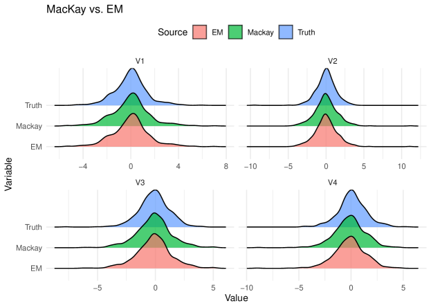
Figure 1: Comparison of the densities for $\bm{\hat{s}}$ and $\bm{s}$

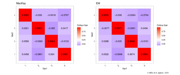
Figure 2: Correlations between $\bm{\hat{s}}$ and $\bm{s}$

Now, we scale the first $\tau$ by 100x and setting $\sigma=0.1$ in the data generating process (26), and repeat the comparisons. Now, both EM algorithm and MacKay’s algorithm has difficulty in identifying the first signal but can identify the rest and performs quite similarly. Figures 3 and 4 show the density estimates and the correlations.

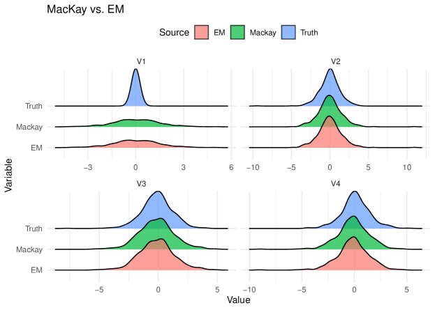
Figure 3: Comparison of the densities for $\bm{\hat{s}}$ and $\bm{s}$

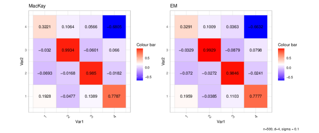
Figure 4: Correlations between $\bm{\hat{s}}$ and $\bm{s}$

6 Discussion

High dimensional feature extraction has been a central tool in many modern day applications. Pattern matching methods such as deep learning compose nonlinear maps to find features. Nonlinear ICA methods can be notoriously hard to learn and recently combinations of flow-based methods and ICA have been used. We have developed a framework for optimization and posterior simulation using auxiliary-based methods. Our proposed method utilize the normal scale mixture representation of the $1/\cosh$ function with Pólya-Gammamixing density. This representation makes it possible to implement both MCMC for fully Bayes inference as well as EM for MAP estimation. This representation also establishes connections with extant literature such as (MacKay,, 1992), (Ono and Miyabe,, 2010) for auxiliary methods, and Bayesian schemes such as (Févotte et al.,, 2004), and others. This is a fruitful area for future research and implementation of fully Bayesian methods.

References

- Andrews and Mallows, (1974) Andrews, D. F. and Mallows, C. L. (1974). Scale mixtures of normal distributions. J. Roy. Statist. Soc. Ser. B, 36:99–102.
- Barlow, (2001) Barlow, H. (2001). Redundancy reduction revisited. Network: computation in neural systems, 12(3):241.
- Barlow, (1989) Barlow, H. B. (1989). Unsupervised learning. Neural computation, 1(3):295–311.
- Barndorff-Nielsen et al., (1982) Barndorff-Nielsen, O., Kent, J., and Sørensen, M. (1982). Normal variance-mean mixtures and distributions. International Statistical Review, 50:145–159.
- Behrmann et al., (2021) Behrmann, J., Vicol, P., Wang, K.-C., Grosse, R., and Jacobsen, J.-H. (2021). Understanding and mitigating exploding inverses in invertible neural networks. In International Conference on Artificial Intelligence and Statistics, pages 1792–1800. PMLR.
- Bell and Sejnowski, (1994) Bell, A. and Sejnowski, T. J. (1994). A non-linear information maximisation algorithm that performs blind separation. Advances in neural information processing systems, 7.
- Bell and Sejnowski, (1995) Bell, A. J. and Sejnowski, T. J. (1995). An information-maximization approach to blind separation and blind deconvolution. Neural computation, 7(6):1129–1159.
- Bhaskara et al., (2014) Bhaskara, A., Charikar, M., and Vijayaraghavan, A. (2014). Uniqueness of tensor decompositions with applications to polynomial identifiability. In Conference on Learning Theory, pages 742–778. PMLR.
- Bouchard, (2007) Bouchard, G. (2007). Efficient bounds for the softmax function and applications to approximate inference in hybrid models. In NIPS 2007 workshop for approximate Bayesian inference in continuous/hybrid systems, volume 6.
- Brillinger, (2012) Brillinger, D. R. (2012). A Generalized Linear Model With “Gaussian” Regressor Variables. In Guttorp, P. and Brillinger, D., editors, Selected Works of David Brillinger, Selected Works in Probability and Statistics, pages 589–606. Springer, New York, NY.
- Camuto et al., (2021) Camuto, A., Willetts, M., Roberts, S., Holmes, C., and Rainforth, T. (2021). Towards a theoretical understanding of the robustness of variational autoencoders. In International Conference on Artificial Intelligence and Statistics, pages 3565–3573. PMLR.
- Carlin and Polson, (1991) Carlin, B. P. and Polson, N. G. (1991). Inference for nonconjugate bayesian models using the gibbs sampler. Canadian Journal of statistics, 19(4):399–405.
- Carvalho et al., (2010) Carvalho, C. M., Polson, N. G., and Scott, J. G. (2010). The horseshoe estimator for sparse signals. Biometrika, 97:465–480.
- Comon, (1994) Comon, P. (1994). Independent component analysis, a new concept? Signal processing, 36(3):287–314.
- Comon et al., (1991) Comon, P., Jutten, C., and Herault, J. (1991). Blind separation of sources, part ii: Problems statement. Signal processing, 24(1):11–20.
- Deco and Obradovic, (1996) Deco, G. and Obradovic, D. (1996). An information-theoretic approach to neural computing. Springer Science & Business Media.
- Detommaso et al., (2019) Detommaso, G., Kruse, J., Ardizzone, L., Rother, C., Köthe, U., and Scheichl, R. (2019). Hint: Hierarchical invertible neural transport for general and sequential bayesian inference. stat, 1050:25.
- Dinh et al., (2014) Dinh, L., Krueger, D., and Bengio, Y. (2014). Nice: Non-linear independent components estimation. arXiv preprint arXiv:1410.8516.
- Dinh et al., (2016) Dinh, L., Sohl-Dickstein, J., and Bengio, S. (2016). Density estimation using real nvp. arXiv preprint arXiv:1605.08803.
- Donnat et al., (2019) Donnat, C., Tozzi, L., and Holmes, S. (2019). Constrained bayesian ica for brain connectome inference. arXiv preprint arXiv:1911.05770.
- Févotte and Godsill, (2006) Févotte, C. and Godsill, S. J. (2006). Blind separation of sparse sources using jeffrey’s inverse prior and the em algorithm. In International Conference on Independent Component Analysis and Signal Separation, pages 593–600. Springer.
- Févotte et al., (2004) Févotte, C., Godsill, S. J., and Wolfe, P. J. (2004). Bayesian approach for blind separation of underdetermined mixtures of sparse sources. In Independent Component Analysis and Blind Signal Separation: Fifth International Conference, ICA 2004, Granada, Spain, September 22-24, 2004. Proceedings 5, pages 398–405. Springer.
- Geman and Yang, (1995) Geman, D. and Yang, C. (1995). Nonlinear image recovery with half-quadratic regularization. IEEE transactions on Image Processing, 4(7):932–946.
- Herault and Jutten, (1986) Herault, J. and Jutten, C. (1986). Space or time adaptive signal processing by neural network models. In AIP conference proceedings, volume 151, pages 206–211. American Institute of Physics.
- Hinton et al., (2001) Hinton, G. E., Welling, M., Teh, Y. W., and Osindero, S. (2001). A new view of ica. In Proceedings of 3rd International Conference on Independent Component Analysis and Blind Signal Separation (ICA’01), pages 746–751.
- Hyvärinen and Pajunen, (1999) Hyvärinen, A. and Pajunen, P. (1999). Nonlinear independent component analysis: Existence and uniqueness results. Neural networks, 12(3):429–439.
- Jaakkola and Jordan, (1997) Jaakkola, T. S. and Jordan, M. I. (1997). A variational approach to bayesian logistic regression models and their extensions. In Sixth International Workshop on Artificial Intelligence and Statistics, pages 283–294. PMLR.
- Jacobsen et al., (2018) Jacobsen, J.-H., Smeulders, A., and Oyallon, E. (2018). i-revnet: Deep invertible networks. arXiv preprint arXiv:1802.07088.
- Jimenez Rezende and Mohamed, (2015) Jimenez Rezende, D. and Mohamed, S. (2015). Variational inference with normalizing flows. arXiv e-prints, pages arXiv–1505.
- Khemakhem et al., (2020) Khemakhem, I., Kingma, D., Monti, R., and Hyvarinen, A. (2020). Variational autoencoders and nonlinear ica: A unifying framework. In International Conference on Artificial Intelligence and Statistics, pages 2207–2217. PMLR.
- Kruse et al., (2021) Kruse, J., Detommaso, G., Köthe, U., and Scheichl, R. (2021). Hint: Hierarchical invertible neural transport for density estimation and bayesian inference. In Proceedings of the AAAI Conference on Artificial Intelligence, volume 35, pages 8191–8199.
- Kruskal, (1977) Kruskal, J. B. (1977). Three-way arrays: rank and uniqueness of trilinear decompositions, with application to arithmetic complexity and statistics. Linear algebra and its applications, 18(2):95–138.
- Li, (1991) Li, K.-C. (1991). Sliced inverse regression for dimension reduction. Journal of the American Statistical Association, 86(414):316–327.
- Lopes et al., (2012) Lopes, H. F., Polson, N. G., and Carvalho, C. M. (2012). Bayesian statistics with a smile: A resampling–sampling perspective.
- MacKay, (1992) MacKay, D. J. (1992). Bayesian interpolation. Neural computation, 4(3):415–447.
- MacKay, (1996) MacKay, D. J. (1996). Maximum likelihood and covariant algorithms for independent component analysis.
- Malthouse, (1998) Malthouse, E. C. (1998). Limitations of nonlinear pca as performed with generic neural networks. IEEE Transactions on neural networks, 9(1):165–173.
- Müller et al., (2019) Müller, T., McWilliams, B., Rousselle, F., Gross, M., and Novák, J. (2019). Neural importance sampling. ACM Transactions on Graphics (ToG), 38(5):1–19.
- Naik and Tsai, (2000) Naik, P. and Tsai, C.-L. (2000). Partial least squares estimator for single-index models. Journal of the Royal Statistical Society: Series B (Statistical Methodology), 62(4):763–771.
- Obradovic and Deco, (1998) Obradovic, D. and Deco, G. (1998). Information maximization and independent component analysis: Is there a difference? Neural Computation, 10(8):2085–2101.
- Olshausen and Field, (1996) Olshausen, B. A. and Field, D. J. (1996). Emergence of simple-cell receptive field properties by learning a sparse code for natural images. Nature, 381(6583):607–609.
- Olshausen and Field, (1997) Olshausen, B. A. and Field, D. J. (1997). Sparse coding with an overcomplete basis set: A strategy employed by v1? Vision research, 37(23):3311–3325.
- Ono and Miyabe, (2010) Ono, N. and Miyabe, S. (2010). Auxiliary-function-based independent component analysis for super-gaussian sources. In International Conference on Latent Variable Analysis and Signal Separation, pages 165–172. Springer.
- Palmer et al., (2006) Palmer, J. A., Kreutz-Delgado, K., and Makeig, S. (2006). Super-gaussian mixture source model for ica. In International Conference on Independent Component Analysis and Signal Separation, pages 854–861. Springer.
- Park and Casella, (2008) Park, T. and Casella, G. (2008). The bayesian lasso. Journal of the American Statistical Association, 103(482):681–686.
- Pearlmutter and Parra, (1996) Pearlmutter, B. A. and Parra, L. C. (1996). A context-sensitive generalization of ica. Advances in neural information processing systems, 151.
- Polson and Sokolov, (2020) Polson, N. and Sokolov, V. (2020). Deep learning: Computational aspects. Wiley Interdisciplinary Reviews: Computational Statistics, 12(5):e1500.
- Polson and Scott, (2016) Polson, N. G. and Scott, J. G. (2016). Mixtures, envelopes and hierarchical duality. Journal of the Royal Statistical Society. Series B, 78:701–727.
- Polson et al., (2013) Polson, N. G., Scott, J. G., and Windle, J. (2013). Bayesian inference for logistic models using pólya–gamma latent variables. Journal of the American statistical Association, 108(504):1339–1349.
- Polson and Sokolov, (2017) Polson, N. G. and Sokolov, V. (2017). Deep learning: A bayesian perspective. Bayesian Analysis, 12(4):1275–1304.
- Saleh and Saleh, (2022) Saleh, R. A. and Saleh, A. (2022). Statistical properties of the log-cosh loss function used in machine learning. arXiv preprint arXiv:2208.04564.
- Samworth and Yuan, (2012) Samworth, R. J. and Yuan, M. (2012). Independent component analysis via nonparametric maximum likelihood estimation. The Annals of Statistics, 40(6):2973–3002.
- Song et al., (2019) Song, Y., Meng, C., and Ermon, S. (2019). Mintnet: Building invertible neural networks with masked convolutions. Advances in Neural Information Processing Systems, 32.
- Tibshirani, (1996) Tibshirani, R. (1996). Regression Shrinkage and Selection via the Lasso. Journal of the Royal Statistical Society. Series B, 58:267–288.
- Trippe and Turner, (2018) Trippe, B. L. and Turner, R. E. (2018). Conditional density estimation with bayesian normalising flows. arXiv preprint arXiv:1802.04908.
- Wang et al., (2023) Wang, Y., Polson, N., and Sokolov, V. O. (2023). Data augmentation for bayesian deep learning. Bayesian Analysis, 18(4):1041–1069.
- West, (1987) West, M. (1987). On scale mixtures of normal distributions. Biometrika, 74(3):646–648.