Thermal Dark Matter with Low-Temperature Reheating

Abstract

We explore the production of thermal dark matter (DM) candidates (WIMPs, SIMPs, ELDERs and Cannibals) during cosmic reheating. Assuming a general parametrization for the scaling of the inflaton energy density and the standard model (SM) temperature, we study the requirements for kinetic and chemical DM freeze-out in a model-independent way. For each of the mechanisms, up to two solutions that fit the entire observed DM relic density exist, for a given reheating scenario and DM mass. As an example, we assume a simple particle physics model in which DM interacts with itself and with SM through contact interactions. We find that low-temperature reheating can accommodate a wider range of couplings and larger masses than those permitted in the usual instantaneous high-temperature reheating. This results in DM solutions for WIMPs reaching masses as high as $10^{14}$ GeV, whereas for SIMPs and ELDERs, we can reach masses of $10^{13}$ GeV. Interestingly, current experimental data already constrain the enlarged parameter space of these models with low-reheating temperatures. Next-generation experiments could further probe these scenarios.

1 Introduction

The evidence for the presence of nonbaryonic dark matter (DM) in the Universe is strongly supported by both astrophysical and cosmological data. For a DM candidate to be considered viable, it must meet several criteria: It must be electromagnetically neutral, cosmologically stable, and nonrelativistic at the time of Big Bang nucleosynthesis (BBN). Additionally, it should exhibit a relic density of $\Omega h^{2}\simeq 0.12$, which accounts for 27% of the total energy content of the Universe [1]; for a recent review see Ref. [2].

The most popular mechanism for DM production in the early Universe is the weakly interacting massive particle (WIMP) model. In this case, DM possesses a mass at the electroweak scale and couples significantly with the standard model (SM) thermal plasma, as is common in electroweak interactions. WIMPs achieve thermal equilibrium with the SM thermal plasma and subsequently undergo chemical freeze-out, leading to the observed DM relic abundance. It is generally assumed that this freeze-out occurs well after reheating has ended, at a time when the Universe’s energy density is dominated by SM radiation. Observational data typically require a thermally averaged annihilation cross-section $\langle\sigma v\rangle\simeq\text{few}\times 10^{-26}$ cm³/s [3]. The WIMP paradigm can have different realizations: one can imagine 2-to-2 annihilation of DM particles into SM states [4], the co-annihilation of a pair of states of the dark sector with only one being the DM [5], or even the semi-annihilation of DM particles into a DM and a SM states [6, 7, 8, 9, 10]. The WIMP mechanism is notably intriguing, as it can be explored through various complementary techniques such as direct, indirect, and collider probes. However, the absence of positive experimental results and strict constraints on its expected parameter space urge investigations beyond the conventional WIMP framework [11, 12, 13].

Alternatively, instead of WIMPs, one can consider the Strongly Interacting Massive Particle (SIMP) paradigm [14] where the freeze-out proceeds through $N$-to-$N^{\prime}$ number-changing processes, where $N$ DM particles annihilate into $N^{\prime}$ of them (with $N>N^{\prime}\geq 2$). The most studied cases of the $N$-to-$N^{\prime}$ processes correspond to 3-to-2, because it is typically dominant. However, 3-to-2 annihilations, necessarily induced by interaction vertices with an odd number of DM particles, are forbidden in the most common models where the stability of the DM is guaranteed by a $\mathbb{Z}_{2}$ symmetry. To allow 3-to-2 annihilations, one has to assume that DM is protected by a different symmetry such as $\mathbb{Z}_{3}$ [15, 16, 17, 18, 19, 20], or consider models where DM stability emerges as a result of DM dynamics [21, 22, 23, 24, 25]. If DM is stabilized by a $\mathbb{Z}_{2}$ symmetry, the 4-to-2 reactions would be those that give rise to the DM relic abundance, while the 3-to-2 annihilations are forbidden [26, 27, 28, 29, 30]. One potential problem of this mechanism is that when $N$-to-$N^{\prime}$ annihilations are effective, the DM reheats itself, significantly modifying the formation of structures [31]. However, this can be avoided by imposing kinetic equilibrium between the DM and the visible sector [14]. In the SIMP paradigm, kinetic equilibrium is broken after chemical equilibrium, so that during DM production, the visible and dark sectors share the same temperature.

However, the kinetic equilibrium could be broken before chemical equilibrium. On the one hand, if this happens when DM is non-relativistic, it corresponds to an ELastically DEcoupling Relic (ELDER) [32, 33]. In this case, at the moment of chemical freeze-out, the DM is warmer than the SM because of efficient $N$-to-$N^{\prime}$ annihilations that tend to keep the DM at a constant temperature as the Universe expands. Interestingly, the near-constant temperature (and therefore density) of DM implies that its present relic abundance is mainly determined by the cross section of its elastic scattering on SM particles (instead of the inelastic processes as in the case of WIMPs or SIMPs).

On the other hand, the scenario where DM goes out of kinetic equilibrium at a very high temperature when it is still relativistic, before breaking the chemical equilibrium corresponds to cannibal or self-interacting DM [34, 35, 36]. In this case, the increase in temperature of the dark sector with respect to the visible sector (occurring between the moment when DM becomes nonrelativistic and its chemical freeze-out) is maximal. In contrast to ELDERs, for cannibal DM, the present relic abundance becomes independent of the detail of kinetic decoupling and is only determined by the chemical freeze-out.

Interestingly, all previously presented thermal production mechanisms can be organized as a function of the temperatures at which DM departs from chemical and kinetic equilibrium. Calling $T_{\text{k}}$ the temperature of SM at kinetic decoupling and $T^{\prime}_{\text{fo}}$ the temperature of DM at chemical decoupling, the WIMP and SIMP scenarios correspond to $m>T^{\prime}_{\text{fo}}>T_{\text{k}}$, ELDER to $m>T_{\text{k}}>T^{\prime}_{\text{fo}}$ and cannibal DM to $T_{\text{k}}>m>T^{\prime}_{\text{fo}}$, where $m$ stands for the mass of the DM particle. We note that since we are interested in cold DM, the hierarchy $m\gg T^{\prime}_{\text{fo}}$ is required.

It is important to note that the present DM abundance is determined not only by the particle-physics dynamics but also by the cosmological history of the Universe. As the evolution of the early Universe is largely unknown, the standard (i.e., the simplest!) assumption corresponds to a Universe dominated by SM radiation from the end of cosmological inflation until matter-radiation equality at a SM temperature $T\simeq 0.8$ eV [1]. Additionally, the transition from an inflaton-dominated to a radiation-dominated Universe, that is, the reheating era, is typically assumed to be instantaneous and to occur at a very high temperature, well before the production of DM. However, this picture cannot be taken for granted. In fact, many well-motivated non-standard deviations could have been realized by nature and therefore should be studied [44]. The reheating temperature $T_{\text{rh}}$ (that is, the SM temperature from which the Universe begins to be dominated by SM radiation) must satisfy $T_{\text{rh}}>T_{\text{bbn}}\simeq 4$ MeV [45, 46, 47, 48, 49], in order not to spoil the success of BBN. The production of DM in scenarios with a nonstandard expansion phase has recently gained increasing interest, particularly for WIMPs [50, 51, 52, 53, 54, 55, 56, 57, 58, 59, 60, 61, 62, 63, 64, 65, 66, 67, 68, 69, 70, 71, 72, 73, 74, 75, 76, 77, 78, 79, 80, 81, 82, 83, 84, 85, 86, 87, 88, 89], but also for SIMPs [90, 91, 88].

During reheating the Universe is dominated by the inflaton. Its energy density is typically assumed to scale as non-relativistic matter or as radiation, corresponding to cases where the inflaton oscillates on a quadratic or quartic potential, respectively. However, it can also scale faster than radiation, as in the case of kination [92, 93], or even faster, as in the context of ekpyrotic [94, 95] or cyclic scenarios [96, 97, 98, 99]; see also Ref. [100]. Additionally, the inflaton could decay or annihilate into different kinds of SM particles, and therefore the dependence of the temperature of the SM bath could feature different behaviors with the cosmic scale factor.

Here, we focus on thermal DM production that occurs during low-temperature reheating. In particular, we study the phenomenology of the thermal production mechanisms mentioned above (WIMP, SIMP, ELDER, and cannibal DM) in the case where kinetic and/or chemical decoupling does not occur in the SM radiation-dominated era but during reheating. For that, in Section 2 we present the general parameterization used to describe the low-temperature reheating scenario. In Section 3, the different thermal DM production mechanisms are presented, highlighting how thermal decoupling occurs, for the usual case where the reheating temperature is very high, much higher than the scales at which the DM is produced. The case in which DM is thermally produced during reheating is studied in Section 4. In Section 5, a simplified particle physics model is presented as an example to materialize our findings. Finally, in Section 6 we summarize and conclude.

2 Low-Temperature Reheating

Cosmic reheating is the era in which the Universe transits from being dominated by inflaton to SM radiation energy density. During reheating, the inflaton $\phi$ has an effective equation of state $\omega$, which implies that its energy density $\rho_{\phi}$ scales as

$$\rho_{\phi}(a)\propto a^{-3\,(1+\omega)},$$ (2.1)

where $a$ corresponds to the cosmic scale factor of the Universe. Particularly interesting cases correspond to $\omega=0$, $\omega=1/3$, and $\omega=1$, corresponding to an inflaton oscillating in a quadratic or quartic potential, and to kination, respectively. More generally, if the inflaton oscillates at the bottom of a monomial potential $V(\phi)\propto\phi^{n}$, its equation of state tends to be $\omega=(n-2)/(n+2)$ [101]. In the case where $\omega>1/3$, $\rho_{\phi}(a)$ gets diluted faster than free radiation and, therefore, eventually the SM energy density dominates without the decay or annihilation of the inflatons. However, if $\omega\leq 1/3$, $\phi$ has to decay or annihilate, injecting entropy into SM particles. We assume that the inflaton only decays or annihilates into SM states, producing a scaling of the SM temperature

$$T(a)=T_{\text{rh}}\left(\frac{a_{\text{rh}}}{a}\right)^{\alpha},$$ (2.2)

where $T_{\text{rh}}$ is the bath temperature at the end of reheating, and the corresponding scale factor $a_{\text{rh}}\equiv a(T_{\text{rh}})$. Furthermore, $\alpha$ depends on the properties of the inflaton during reheating. For an inflaton oscillating in a quadratic potential ($\omega=0$) and a constant decay width, $\alpha=3/8$. However, even in the case of $\omega=0$, other scalings are possible, for example, in the case of a nontrivial dependence of the decay width of the inflaton with the scale factor [104, 105, 106, 107, 108, 109, 110, 111, 112]. Interestingly, in a quadratic potential, one can also have an era with constant temperature $\alpha=0$, as elaborated in Refs. [113, 107, 114]. Alternatively, if the inflaton oscillates in a quartic potential ($\omega=1/3$), the decay into scalar or fermionic states gives rise to $\alpha=1/4$ or 3/4, respectively. In general, in the case of a monomial potential $\alpha=\frac{3}{2}\,\frac{1}{2+n}$ for a scalar decay, and $\alpha=\frac{3}{2}\,\frac{n-1}{2+n}$ if $n\leq 7$ or $\alpha=1$ if $n\geq 7$ for a fermionic decay [115, 116, 86]. If instead of decaying, reheating occurs through inflaton annihilations into bosons, one gets $\alpha=\frac{9}{2\,n+4}$ for $n\geq 3$ or $\alpha=\frac{3(7-2n)}{2\,n+4}$, for the case of a heavy or light mediator, respectively [117, 118]. The case of inflaton annihilations into fermions gives $\alpha=1$ or $\alpha=\frac{3(5-n)}{2\,n+4}$, for a heavy or light mediator, respectively [118]. Finally, if the inflaton energy density is diluted faster than free radiation, that is, if $\omega>1/3$, it is not necessary for the inflaton to decay or annihilate away, and then one can have $\alpha=1$, as in the case of kination [92, 93]. We note that, in cases where $\alpha>0$, during reheating the SM bath temperature rises to a maximal value $T_{\text{max}}$ that could exceed $T_{\text{rh}}$ by several orders of magnitude [119].

Taking into account that the SM radiation energy density $\rho_{R}$ is given by

$$\rho_{R}(T)=\frac{\pi^{2}}{30}\,g_{\star}(T)\,T^{4},$$ (2.3)

with $g_{\star}(T)$ being the number of relativistic degrees of freedom contributing to $\rho_{R}$ [120], it is interesting to note that a viable reheating, that is, an eventual onset of the SM radiation domination, requires that at some point $\rho_{R}(a)>\rho_{\phi}(a)$, which in turn implies

$$\alpha\leq\frac{3}{4}\,(1+\omega)\,.$$ (2.4)

In the plane $[\omega,\,\alpha]$, Fig. 1 shows with crosses the different reheating options previously discussed. The black dot corresponds to the standard case with $\omega=0$ and $\alpha=3/8$. The thin black dotted lines correspond to the previously described scenarios: the vertical one to $\omega=0$ (dust-like inflaton), the horizontal one to a kination-like faster-than-radiation expansion, and the five diagonals to decay and annihilations into scalars and fermions. Importantly, the red area in the upper left corner does not give rise to a viable reheating, cf. Eq. (2.4), and is therefore ignored.

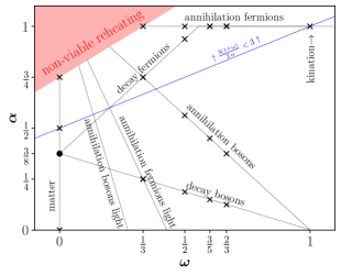
Figure 1: Summary of the different reheating scenarios. The black dot corresponds to the standard case where the inflaton scales as non-relativistic matter and decays into SM particles with a constant decay width, while the black crosses correspond to the alternatives described in the text. The red area in the upper left corner does not give rise to viable reheating. Above the blue dotted line $\frac{3(1+\omega)}{2\,\alpha}<3$.

The Hubble expansion rate $H$ depends on the total energy density of the Universe and is given by the Friedmann equation

$$H^{2}=\frac{\rho_{\phi}+\rho_{R}}{3\,M_{P}^{2}}\,,$$ (2.5)

where $M_{P}\simeq 2.4\times 10^{18}$ GeV is the reduced Planck mass. It can be approximately written as

$$H(a)\simeq H(a_{\text{rh}})\times\begin{dcases}\left(\frac{a_{\text{rh}}}{a}\right)^{\frac{3\,(1+\omega)}{2}}&\text{ for }a\leq a_{\text{rh}},\\ \left(\frac{a_{\text{rh}}}{a}\right)^{2}&\text{ for }a_{\text{rh}}\leq a,\end{dcases}$$ (2.6)

depending on whether we are during ($a\leq a_{\text{rh}}$) or after ($a\geq a_{\text{rh}}$) reheating, which corresponds to

$$H(T)\simeq H(T_{\text{rh}})\times\begin{dcases}\left(\frac{T}{T_{\text{rh}}}\right)^{\frac{3\,(1+\omega)}{2\,\alpha}}&\text{ for }T\geq T_{\text{rh}},\\ \left(\frac{T}{T_{\text{rh}}}\right)^{2}&\text{ for }T_{\text{rh}}\geq T,\end{dcases}$$ (2.7)

where the reheating temperature $T_{\text{rh}}$ is implicitly defined by the equality $\rho_{\phi}(T_{\text{rh}})=\rho_{R}(T_{\text{rh}})$. We note that if $\frac{3(1+\omega)}{2\alpha}=2$, $H$ has the same scaling with temperature during and after reheating.

3 Dark Matter Production After Reheating

In this section, different thermal production mechanisms for DM in the early Universe are studied, assuming the standard scenario where the reheating temperature is much higher than the relevant scales for DM genesis. The two cases $T_{\text{fo}}\gg T_{\text{k}}$ (corresponding to WIMPs and SIMPs) and $T_{\text{k}}\gg T_{\text{fo}}$ (corresponding to ELDERs and cannibals) are studied separately.

3.1 WIMPs and SIMPs: $T_{\text{rh}}\gg T_{\text{fo}}\gg T_{\text{k}}$

Both in the WIMP and the SIMP paradigms, chemical equilibrium is broken before kinetic equilibrium, $T_{\text{fo}}\gg T_{\text{k}}$, which guarantees that at chemical freeze-out the two sectors share the same temperature $T$.

The equilibrium number density $n_{\text{eq}}$ for DM particles of mass $m$ and $g$ internal degrees of freedom is given by

$$n_{\text{eq}}(T)=\frac{g}{2\pi^{2}}\,m^{2}\,T\,K_{2}\left(\frac{m}{T}\right),$$ (3.1)

where $K_{i}$ is the modified Bessel function, and where the Maxwell-Boltzmann statistic was assumed. For simplicity, in all numerical evaluations we fix $g=1$. After chemical freeze-out, the DM yield defined as $Y(T)\equiv n(T)/s(T)$ is conserved, where $n(T)$ is the DM number density,

$$s(T)\equiv\frac{2\pi^{2}}{45}\,g_{\star s}(T)\,T^{3}$$ (3.2)

is the SM entropy density, and $g_{\star s}(T)$ corresponds to the effective number of degrees of freedom contributing to the SM entropy [120]. At present, the DM yield $Y_{0}$ can be estimated as

$$Y_{0}\simeq Y_{\text{fo}}=\frac{n_{\text{eq}}(T_{\text{fo}})}{s(T_{\text{fo}})}=\frac{45}{4\pi^{4}}\,\frac{g}{g_{\star s}(T_{\text{fo}})}\,x_{\text{fo}}^{2}\,K_{2}(x_{\text{fo}})\simeq\frac{45}{2^{5/2}\,\pi^{7/2}}\,\frac{g}{g_{\star s}(T_{\text{fo}})}\,x_{\text{fo}}^{3/2}\,e^{-x_{\text{fo}}},$$ (3.3)

with $x_{\text{fo}}\equiv m/T_{\text{fo}}$. We emphasize that at this level, WIMPs and SIMPs are indistinguishable, as the reaction fixing the DM freeze-out has not been specified.

To match the entire observed DM relic density, it is required that

$$m\,Y_{0}=\frac{\Omega h^{2}\,\rho_{c}}{s_{0}\,h^{2}}\simeq 4.3\times 10^{-10}~{}\text{GeV},$$ (3.4)

where $Y_{0}$ is the asymptotic value of the DM yield at low temperatures, $s_{0}\simeq 2.69\times 10^{3}$ cm^-3 is the present entropy density [121], $\rho_{c}\simeq 1.05\times 10^{-5}~{}h^{2}$ GeV/cm³ is the critical energy density of the Universe, and $\Omega h^{2}\simeq 0.12$ is the observed DM relic abundance [1]. Figure 2 shows, for different DM masses, the parameter space that fits the observed DM relic abundance, in an extravagantly large plane $[{x^{\prime}_{\text{fo}}},\,x_{\text{k}}]$. We recall that in this case ${x^{\prime}_{\text{fo}}}=x_{\text{fo}}$, given that for WIMPs and SIMPs $T_{\text{fo}}\gg T_{\text{k}}$. As expected from Eq. (3.3), the DM relic abundance is independent of the kinetic decoupling (i.e. the lines are vertical) and has a small logarithmic dependence on the DM mass. In the red band, corresponding to ${x^{\prime}_{\text{fo}}}<3$, DM freezes-out when still relativistic, and therefore it is not a cold relic.

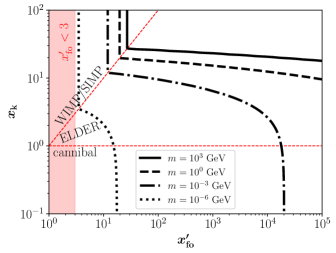
Figure 2: Parameter space that fits the observed DM relic abundance for different DM masses, assuming a production after reheating (that is, in the radiation-dominated era). In the red band (${x^{\prime}_{\text{fo}}}<3$), DM freezes-out when relativistic, and is therefore not a cold relic.

3.2 Cannibals and ELDERs: $T_{\text{rh}}\gg T_{\text{k}}\gg T_{\text{fo}}$

Opposite to the WIMP and the SIMP cases, for ELDERs and cannibals kinetic equilibrium is broken before chemical equilibrium, $T_{\text{k}}\gg T_{\text{fo}}$. It is important to note that kinetic equilibrium guarantees that the two sectors have a common temperature and therefore if it is broken, the two sectors will be characterized by different temperatures: $T$ for the SM and $T^{\prime}$ for the dark sector.

The DM yield at chemical freeze-out is given by

$$Y_{\text{fo}}=\frac{n_{\text{eq}}(T^{\prime}_{\text{fo}})}{s(T_{\text{fo}})}=\frac{n_{\text{eq}}(T^{\prime}_{\text{fo}})}{s(T_{\text{k}})}\,\frac{s^{\prime}(T_{\text{k}})}{s^{\prime}(T^{\prime}_{\text{fo}})}\,,$$ (3.5)

where in the first equality we have used the fact that at freeze out the DM has a temperature $T^{\prime}_{\text{fo}}$ while the SM temperature is $T_{\text{fo}}$, while in the second, the separate conservation of the entropies of the visible and dark sectors ($s$ and $s^{\prime}$ respectively) was taken into account. Additionally, given that the energy density $\rho^{\prime}$ and the pressure $p^{\prime}$ of the dark sector are

$$\rho^{\prime}(T^{\prime}) =\frac{g}{2\pi^{2}}\,m^{3}\,T^{\prime}\left[K_{1}\left(\frac{m}{T^{\prime}}\right)+3\,\frac{T^{\prime}}{m}\,K_{2}\left(\frac{m}{T^{\prime}}\right)\right],$$ (3.6)

$$p^{\prime}(T^{\prime}) =\frac{g}{2\pi^{2}}\,m^{2}\,{T^{\prime}}^{2}\,K_{2}\left(\frac{m}{T^{\prime}}\right),$$ (3.7)

for a Maxwell-Boltzmann distribution without chemical potential, the entropy density of the dark sector can be written as

$$s^{\prime}(T^{\prime})=\frac{\rho^{\prime}(T^{\prime})+p^{\prime}(T^{\prime})}{T^{\prime}}=\frac{g}{2\pi^{2}}\,m^{3}\,K_{3}\left(\frac{m}{T^{\prime}}\right).$$ (3.8)

Therefore, the DM yield at present can be conveniently expressed as

$$Y_{0}\simeq Y_{\text{fo}}=\frac{45}{4\pi^{4}}\,\frac{g}{g_{\star s}(T_{\text{k}})}\,\frac{x_{\text{k}}^{3}}{{x^{\prime}_{\text{fo}}}}\,\frac{K_{2}({x^{\prime}_{\text{fo}}})\,K_{3}(x_{\text{k}})}{K_{3}({x^{\prime}_{\text{fo}}})}\,,$$ (3.9)

with $x_{\text{k}}\equiv m/T_{\text{k}}$ and ${x^{\prime}_{\text{fo}}}\equiv m/T^{\prime}_{\text{fo}}$. As expected, Eqs. (3.9) and (3.3) coincide in the limit $x_{\text{k}}=x_{\text{fo}}={x^{\prime}_{\text{fo}}}$. Figure  2 also displays the parameter space that fits the observed abundance of DM, for the case ${x^{\prime}_{\text{fo}}}>x_{\text{k}}$.

Equation (3.9) has two interesting limits extensively discussed in the literature. The case where chemical decoupling occurs non-relativistically, but kinetic decoupling when DM is still relativistic ($x_{\text{k}}\ll 1\ll{x^{\prime}_{\text{fo}}}$) corresponds to the cannibal scenario, and therefore Eq. (3.9) reduces to

$$Y_{0}\simeq\frac{90}{\pi^{4}}\,\frac{g}{g_{\star s}(T_{\text{k}})}\,\frac{1}{{x^{\prime}_{\text{fo}}}}\,,$$ (3.10)

and is independent of the kinetic decoupling [34]. Alternatively, if both kinetic and chemical decoupling happen when DM is non-relativistic ($1\ll x_{\text{k}}\ll{x^{\prime}_{\text{fo}}}$)

$$Y_{0}\simeq\frac{45}{2^{5/2}\,\pi^{7/2}}\,\frac{g}{g_{\star s}(T_{\text{k}})}\,\frac{x_{\text{k}}^{5/2}\,e^{-x_{\text{k}}}}{{x^{\prime}_{\text{fo}}}}\,,$$ (3.11)

corresponding to the ELDER scenario [32, 33]. Even if it also depends on ${x^{\prime}_{\text{fo}}}$, the ELDER limit has a strong exponential dependence on the kinetic decoupling. The two regimes can be recognized in Fig. 2.

Before closing this section, we note that the separate conservation of entropies allows us to compute the SM temperature at freeze-out $T_{\text{fo}}$

$$x_{\text{fo}}\equiv\frac{m}{T_{\text{fo}}}=x_{\text{k}}\left[\frac{g_{\star s}(T_{\text{fo}})}{g_{\star s}(T_{\text{k}})}\,\frac{K_{3}(x_{\text{k}})}{K_{3}({x^{\prime}_{\text{fo}}})}\right]^{1/3},$$ (3.12)

as a function of $x_{\text{k}}$ and ${x^{\prime}_{\text{fo}}}$.

4 Dark Matter Production During Reheating

Although it is commonly assumed that cosmic reheating finishes at a very high temperature, it may not be the case. In this section, we study different thermal mechanisms in the case where they are effective during reheating. We emphasize that, by construction, the inflaton transmits its energy to the SM bath and not to the DM. This is typically a good assumption as long as its branching ratio to the dark sector is smaller than $\mathcal{O}(10^{-4})\times m/(100~{}\text{GeV})$ [70, 77].

4.1 WIMPs and SIMPs: $T_{\text{fo}}\gg T_{\text{rh}}$

The impact on the final DM relic abundance produced through the WIMP and the SIMP mechanisms occurring during reheating is two-fold. On the one hand, chemical decoupling occurs earlier, increasing the DM yield; on the other hand, injection of entropy into the SM bath because of inflaton decays dilutes the DM abundance.

The dilution corresponds to the change in SM entropy $S$ from a given moment until the end of the reheating and is given by

$$\frac{S(T)}{S(T_{\text{rh}})}=\frac{s(T)}{s(T_{\text{rh}})}\left(\frac{a(T)}{a(T_{\text{rh}})}\right)^{3}=\frac{g_{\star s}(T)}{g_{\star s}(T_{\text{rh}})}\left(\frac{T_{\text{rh}}}{T}\right)^{\frac{3\,(1-\alpha)}{\alpha}},$$ (4.1)

where Eqs. (2.2) and (3.2) were used. Given that the SM entropy is conserved after the end of reheating, the DM yield at present can be estimated by

$$Y_{0}\simeq Y_{\text{rh}}=Y_{\text{fo}}\,\frac{S(T_{\text{fo}})}{S(T_{\text{rh}})}=\frac{45}{4\pi^{4}}\,\frac{g}{g_{\star s}(T_{\text{rh}})}\,x_{\text{fo}}^{2}\,K_{2}(x_{\text{fo}})\left(\frac{x_{\text{fo}}}{x_{\text{rh}}}\right)^{\frac{3\,(1-\alpha)}{\alpha}},$$ (4.2)

where $Y_{\text{fo}}$ is the same as the one computed in Eq. (3.3). Interestingly, Eq. (4.2) is valid as long as $T_{\text{fo}}>T_{\text{rh}}$, in the two cases $T_{\text{fo}}>T_{\text{rh}}>T_{\text{k}}$ and $T_{\text{fo}}>T_{\text{k}}>T_{\text{rh}}$. Additionally, it can be approximated in the two limits

$$Y_{0}\simeq\begin{dcases}\frac{45}{2\pi^{4}}\,\frac{g}{g_{\star s}(T_{\text{rh}})}\left(\frac{x_{\text{fo}}}{x_{\text{rh}}}\right)^{\frac{3\,(1-\alpha)}{\alpha}}&\text{ for }x_{\text{fo}}\ll x_{\text{fo}}^{\text{c}}\,,\\ \frac{45}{4\pi^{4}}\sqrt{\frac{\pi}{2}}\,\frac{g}{g_{\star s}(T_{\text{rh}})}\,x_{\text{fo}}^{\frac{3}{2}}\,e^{-x_{\text{fo}}}\left(\frac{x_{\text{fo}}}{x_{\text{rh}}}\right)^{\frac{3\,(1-\alpha)}{\alpha}}&\text{ for }x_{\text{fo}}\gg x_{\text{fo}}^{\text{c}}\,,\end{dcases}$$ (4.3)

where the critical value $x_{\text{fo}}^{\text{c}}$ (after extremizing Eq. (4.2) w.r.t. $x_{\text{fo}}$) is implicitly defined by

$$\alpha\,x_{\text{fo}}^{\text{c}}\,K_{1}(x_{\text{fo}}^{\text{c}})+3\,(\alpha-1)\,K_{2}(x_{\text{fo}}^{\text{c}})=0\,.$$ (4.4)

Several comments are in order with respect to Eq. (4.3). $i)$ To be realized, the first expression (corresponding to $x_{\text{fo}}\ll x_{\text{fo}}^{\text{c}}$) requires interaction rates with a higher temperature dependence than the Hubble expansion rate, as will be shown in Section 5. $ii)$ For the second expression (corresponding to $x_{\text{fo}}\gg x_{\text{fo}}^{\text{c}}$) one only has to require $x_{\text{fo}}<x_{\text{rh}}$. And $iii)$, with respect to $x_{\text{fo}}^{\text{c}}$, for a given $T_{\text{rh}}$, a critical value of the DM mass can be defined as the mass required to fit the entire abundance of DM if $x_{\text{fo}}=x_{\text{fo}}^{\text{c}}$. DM with a mass larger than that value overshoots the observations if it is produced during reheating.

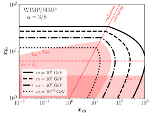
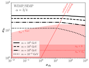
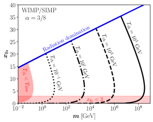
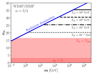
Figure 3: Value of $x_{\text{fo}}$ required to fit the entire DM relic abundance for $\alpha=3/8$ (left) or $\alpha=3/4$ (right), as a function of $x_{\text{rh}}$ (top) or $m$ (bottom), in the WIMP and SIMP scenarios. The red bands are in tension with BBN or the non-relativistic freeze-out.

The parameter space that fits the observed DM relic abundance for WIMPs and SIMPs, taking $\alpha=3/8$ (left) or $\alpha=3/4$ (right), as a function of $x_{\text{rh}}$ (top) or $m$ (bottom), is shown in Fig. 3. The red dotted horizontal lines correspond to the critical value $x_{\text{fo}}^{\text{c}}\simeq 6.2$ (1.9) for $\alpha=3/8$ (3/4), while the red dashed diagonal lines in the upper panel depict the border between freeze-out during radiation domination and reheating (that is, when $x_{\text{fo}}=x_{\text{rh}}$). The red bands are in tension with BBN or the non-relativistic freeze-out. In the upper panels of Fig. 3, if $x_{\text{fo}}>x_{\text{rh}}$, DM freezes out in the radiation-dominated era and therefore the abundance of DM is independent of $x_{\text{rh}}$. In contrast, if $x_{\text{fo}}<x_{\text{rh}}$, DM is produced during reheating, at a higher temperature (that is, smaller $x_{\text{fo}}$) compared to the standard case. For a fixed $x_{\text{rh}}$, the two solutions during reheating described in Eq. (4.3) are visible. Furthermore, the corresponding maximum mass (for a given $T_{\text{rh}}$) clearly appears in the lower left panel of Fig. 3, at $x_{\text{fo}}=x_{\text{fo}}^{\text{c}}$. This novel feature of a double solution during reheating is further investigated in Appendix A, where a complete numerical calculation was performed, solving the system of Boltzmann equations for the inflaton and SM radiation energy densities and the DM number density. Finally, the minimal viable DM mass that can be produced during reheating is also visible, and corresponds to point where $T_{\text{fo}}=T_{\text{rh}}=T_{\text{bbn}}$.

4.2 Cannibals and ELDERs: $T_{\text{k}}\gg T_{\text{fo}}$

This section is conveniently divided into two cases, $T_{\text{rh}}\gg T_{\text{fo}}$ and $T_{\text{fo}}\gg T_{\text{rh}}$, depending on whether reheating finishes after or before the DM chemical freeze-out.

4.2.1 $T_{\text{k}}\gg T_{\text{rh}}\gg T_{\text{fo}}$

In this case where $T_{\text{k}}\gg T_{\text{rh}}\gg T_{\text{fo}}$, the DM yield at present is given by

$$Y_{0} \simeq Y_{\text{fo}}=\frac{n_{\text{eq}}(T^{\prime}_{\text{fo}})}{s(T_{\text{fo}})}=\frac{n_{\text{eq}}(T^{\prime}_{\text{fo}})}{s(T_{\text{rh}})}\,\frac{s^{\prime}(T_{\text{rh}}^{\prime})}{s^{\prime}(T^{\prime}_{\text{fo}})}=\frac{n_{\text{eq}}(T^{\prime}_{\text{fo}})}{s(T_{\text{rh}})}\,\frac{s^{\prime}(T_{\text{k}})}{s^{\prime}(T^{\prime}_{\text{fo}})}\left(\frac{T_{\text{rh}}}{T_{\text{k}}}\right)^{\frac{3}{\alpha}}$$

$$=\frac{45}{4\pi^{4}}\,\frac{g}{g_{\star s}(T_{\text{rh}})}\,\frac{x_{\text{rh}}^{3}}{{x^{\prime}_{\text{fo}}}}\left(\frac{x_{\text{k}}}{x_{\text{rh}}}\right)^{\frac{3}{\alpha}}\frac{K_{2}({x^{\prime}_{\text{fo}}})\,K_{3}(x_{\text{k}})}{K_{3}({x^{\prime}_{\text{fo}}})},$$ (4.5)

where the separate conservation of entropies between the end of reheating and the DM freeze-out, and the scaling of the DM temperature during reheating were used.

In this case where $T_{\text{k}}\gg T_{\text{fo}}$, at the time of chemical freeze out the two sectors are not expected to share the same temperature. Using the conservation of the dark sector entropy between $a(T_{\text{k}})$ and $a_{\text{fo}}$, the conservation of the SM entropy between $a_{\text{rh}}$ and $a_{\text{fo}}$, and the entropy injection in Eq. (4.1), one gets that

$$x_{\text{fo}}=x_{\text{rh}}\left(\frac{x_{\text{k}}}{x_{\text{rh}}}\right)^{\frac{1}{\alpha}}\left[\frac{g_{\star s}(T_{\text{fo}})}{g_{\star s}(T_{\text{rh}})}\,\frac{K_{3}(x_{\text{k}})}{K_{3}({x^{\prime}_{\text{fo}}})}\right]^{\frac{1}{3}}.$$ (4.6)

4.2.2 $T_{\text{k}}\gg T_{\text{fo}}\gg T_{\text{rh}}$

Alternatively, in the case where $T_{\text{k}}\gg T_{\text{fo}}\gg T_{\text{rh}}$, the DM yield at present is given by

$$Y_{0} \simeq Y_{\text{rh}}=\frac{n_{\text{eq}}(T_{\text{rh}}^{\prime})}{s(T_{\text{rh}})}=\frac{n_{\text{eq}}(T^{\prime}_{\text{fo}})}{s(T_{\text{rh}})}\,\frac{s^{\prime}(T_{\text{rh}}^{\prime})}{s^{\prime}(T^{\prime}_{\text{fo}})}=\frac{n_{\text{eq}}(T^{\prime}_{\text{fo}})}{s(T_{\text{rh}})}\,\frac{s^{\prime}(T_{\text{k}})}{s^{\prime}(T^{\prime}_{\text{fo}})}\left(\frac{T_{\text{rh}}}{T_{\text{k}}}\right)^{\frac{3}{\alpha}}$$

$$=\frac{45}{4\pi^{4}}\,\frac{g}{g_{\star s}(T_{\text{rh}})}\,\frac{x_{\text{rh}}^{3}}{{x^{\prime}_{\text{fo}}}}\left(\frac{x_{\text{k}}}{x_{\text{rh}}}\right)^{\frac{3}{\alpha}}\frac{K_{2}({x^{\prime}_{\text{fo}}})\,K_{3}(x_{\text{k}})}{K_{3}({x^{\prime}_{\text{fo}}})}\,,$$ (4.7)

which, as expected, is equal to the expression in Eq. (4.2.1), and simply corresponds to Eq. (3.9) times the dilution factor between $T_{\text{k}}$ and $T_{\text{rh}}$. However, even if the expressions for the DM yield are the same, the SM temperature at which the chemical freeze-out occurs is different. Using the conservation of the dark sector entropy between $a(T_{\text{k}})$ and $a_{\text{fo}}$, and the entropy injection to the visible sector in Eq. (4.1), one gets that the SM temperature at chemical freeze-out is

$$x_{\text{fo}}=x_{\text{k}}\left[\frac{K_{3}(x_{\text{k}})}{K_{3}({x^{\prime}_{\text{fo}}})}\right]^{\frac{\alpha}{3}},$$ (4.8)

independently of the reheating temperature, and which only coincides with Eq. (4.6) in the limit $x_{\text{k}}=x_{\text{fo}}$.

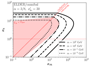
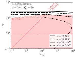
Figure 4: Parameter space that fits the observed DM relic abundance, for ELDERs and cannibals, for $\alpha=3/8$ (left) or $\alpha=3/4$ (right), ${x^{\prime}_{\text{fo}}}=30$ and different DM masses. The red bands are in tension with BBN.

Considering Eq. (4.2.1) (or equivalently Eq. (4.2.2)), the ELDER limit occurs if both kinetic and chemical decoupling happen when DM is non-relativistic ($1\ll x_{\text{k}}\ll{x^{\prime}_{\text{fo}}}$)

$$Y_{0}\simeq\frac{45}{2^{5/2}\,\pi^{7/2}}\,\frac{g}{g_{\star s}(T_{\text{rh}})}\,\frac{x_{\text{k}}^{5/2}\,e^{-x_{\text{k}}}}{{x^{\prime}_{\text{fo}}}}\left(\frac{x_{\text{k}}}{x_{\text{rh}}}\right)^{\frac{3(1-\alpha)}{\alpha}},$$ (4.9)

while in the case where chemical decoupling occurs nonrelativistically, but kinetic decoupling when DM is still relativistic ($x_{\text{k}}\ll 1\ll{x^{\prime}_{\text{fo}}}$) corresponds to the cannibal scenario and therefore the DM yield reduces to

$$Y_{0}\simeq\frac{90}{\pi^{4}}\,\frac{g}{g_{\star s}(T_{\text{rh}})}\,\frac{1}{{x^{\prime}_{\text{fo}}}}\left(\frac{x_{\text{k}}}{x_{\text{rh}}}\right)^{\frac{3(1-\alpha)}{\alpha}},$$ (4.10)

which, contrary to the case in radiation domination, shows a dependence on the kinetic decoupling coming from the dilution factor. The parameter space that fits the observed DM relic abundance for ELDERs and cannibals, taking $\alpha=3/8$ (left) or $\alpha=3/4$ (right), ${x^{\prime}_{\text{fo}}}=30$ and different masses of DM, is shown in Fig. 4. In a way equivalent to WIMPs/SIMPs, if $x_{\text{k}}<x_{\text{rh}}$ DM kinetically decouples during reheating, at a higher temperature (that is, smaller $x_{\text{k}}$) compared to the standard case. Also, for a fixed $x_{\text{rh}}$, two solutions during reheating are visible.

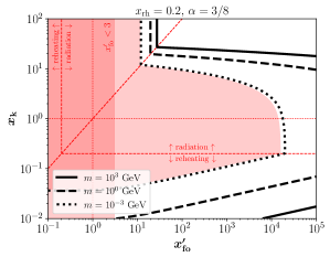
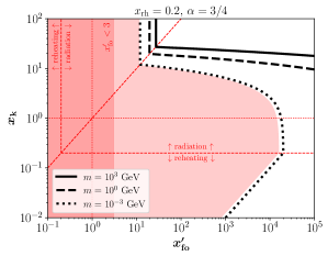
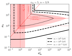
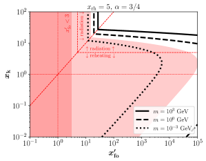
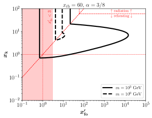
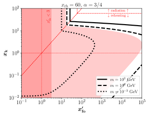
Figure 5: Parameter space that fits the observed DM relic abundance, for different DM masses. For reheating, we assume $\alpha=3/8$ (left) or $\alpha=3/4$ (right), and $x_{\text{rh}}=0.5$ (top), 5 (middle) or 50 (bottom). The thin red dotted lines show $x_{\text{k}}=1$ and ${x^{\prime}_{\text{fo}}}=1$, while the dashed red lines correspond to $x_{\text{k}}={x^{\prime}_{\text{fo}}}$, $x_{\text{k}}=x_{\text{rh}}$, and ${x^{\prime}_{\text{fo}}}=x_{\text{rh}}$. The red bands are in tension with BBN or the non-relativistic freeze-out.

All in all, the previously discussed cases are summarized in Fig. 5, for $\alpha=3/8$ (left) or $\alpha=3/4$ (right) and three reheating temperatures $x_{\text{rh}}=0.2$ (top), $x_{\text{rh}}=5$ (middle), and $x_{\text{rh}}=60$ (bottom); it is equivalent to Fig. 2 but for low-reheating scenarios. The thin red dotted lines show $x_{\text{k}}=1$ and ${x^{\prime}_{\text{fo}}}=1$, while the dashed red lines correspond to $x_{\text{k}}={x^{\prime}_{\text{fo}}}$, $x_{\text{k}}=x_{\text{rh}}$, and ${x^{\prime}_{\text{fo}}}=x_{\text{rh}}$. The red bands are in tension with BBN or the non-relativistic freeze-out. We notice that while in cases $x_{\text{rh}}=0.2$ and $x_{\text{rh}}=5$ there is a single solution during reheating, for $x_{\text{rh}}=60$ and $\alpha=3/8$ the two solutions are reachable. A fully numerical solution of a case where the two solutions occur is presented in Appendix A.

5 Particle Physics Realization

In this section we give a simple example of a specific particle physics model that realizes the previous DM production mechanisms. In the case of contact interactions, the cross sections for the 2-to-2 annihilation of DM into SM particles $\langle\sigma v\rangle_{2\to 2}$ and the elastic scattering of a DM particle with a SM particle $\langle\sigma v\rangle_{\text{el}}$ are given by

$$\langle\sigma v\rangle_{\text{el}}\sim\langle\sigma v\rangle_{2\to 2}\sim\left[\frac{\epsilon_{\text{eff}}}{m}\,\frac{K_{1}(x)}{K_{2}(x)}\right]^{2}\simeq\begin{dcases}\frac{\epsilon_{\text{eff}}^{2}}{4\,T^{2}}&\text{ for }x\ll 1\,,\\ \frac{\epsilon_{\text{eff}}^{2}}{m^{2}}&\text{ for }x\gg 1\,,\end{dcases}$$ (5.1)

as a function of the dimensionless effective coupling $\epsilon_{\text{eff}}$. Additionally, 3-to-2 DM annihilations are characterized by the thermally averaged cross section

$$\langle\sigma v^{2}\rangle_{3\to 2}\sim\frac{y_{\text{eff}}^{3}}{m^{5}}$$ (5.2)

for $x\gg 1$, and depends on the the dimensionless effective coupling $y_{\text{eff}}$. Therefore, the corresponding interaction rates are

$$\Gamma_{\text{el}} =n^{\text{sm}}_{\text{eq}}\,\langle\sigma v\rangle_{\text{el}}\,,$$ (5.3)

$$\Gamma_{2\to 2} =n_{\text{eq}}\,\langle\sigma v\rangle_{2\to 2}\,,$$ (5.4)

$$\Gamma_{3\to 2} =n_{\text{eq}}^{2}\,\langle\sigma v^{2}\rangle_{3\to 2}\,,$$ (5.5)

where $n_{\text{eq}}$ is the DM number density in equilibrium given in Eq. (3.1), and

$$n^{\text{sm}}_{\text{eq}}(T)=\frac{\zeta(3)}{\pi^{2}}\,g_{\text{sm}}\,T^{3}$$ (5.6)

is the equilibrium number density for SM particles, where $g_{\text{sm}}(T)$ is the number of relativistic SM degrees of freedom that interact with DM (each fermionic degree of freedom counts as 3/4 due to statistics), and $\zeta(3)\simeq 1.2$ is the Riemann zeta function. Here we fix $g_{\text{sm}}=2$.

As 3-to-2 DM annihilations are effective, it is expected that elastic 2-to-2 DM self-scattering, with a cross section $\sigma_{\text{dm}}$ in the non-relativistic limit given by

$$\sigma_{\text{dm}}\sim\frac{y_{\text{eff}}^{2}}{m^{2}},$$ (5.7)

is efficient as well. Here, for simplicity, we have assumed the same coupling $y_{\text{eff}}$ for the 3-to-2 and 2-to-2 scatterings. The non-observation of an offset between the mass distributions of DM and hot baryonic gas in the Bullet cluster constrains the ratio of the self-scattering cross section over DM mass to be $\sigma_{\text{dm}}/m<1.25$ cm²/g [126, 127, 128]. Further observations of other cluster collisions reinforce this bound to $\sigma_{\text{dm}}/m<0.2$ - $0.5$ cm²/g [129, 130, 131].

5.1 After Reheating

For the case in which DM is produced well after the end of reheating, Fig. 6 shows with thick black lines the parameter space that fits the entire observed abundance of DM in the case of thermal production after reheating (that is, during radiation domination), for different DM masses. It corresponds to the information in Fig. 2 projected in the plane $[y_{\text{eff}},\,\epsilon_{\text{eff}}]$. The dashed red lines correspond to the boundaries between the different thermal production mechanisms. Several comments are in order: $i)$ The WIMP case depends only on $\epsilon_{\text{eff}}$, and can be realized for a wide range of masses: from few keV (Lyman-$\alpha$ bound [123]) to $\sim 130$ TeV (unitarity bound [132]). However, there is an upper limit for $y_{\text{eff}}$ from which DM becomes a SIMP. $ii)$ Due to the consideration of the perturbativity of $y_{\text{eff}}$, the SIMP and ELDER mechanisms can occur only in the sub-GeV range. $iii)$ SIMPs only depend on $y_{\text{eff}}$. The upper and lower bounds on $\epsilon_{\text{eff}}$ appear to avoid the WIMP and ELDER solutions, respectively. $iv)$ ELDERs depend mainly on $\epsilon_{\text{eff}}$, having only a logarithmic dependence on $y_{\text{eff}}$. $v)$ As a result of the choice of the interaction between the visible and dark sectors (i.e., Eq. (5.1)), and in particular of the suppression of the cross section at large temperatures, the cannibal mechanism cannot be realized. In fact, kinetic equilibrium, given by the equality $\Gamma_{\text{el}}(x_{\text{k}})=H(x_{\text{k}})$, can only occur if $x_{\text{k}}\geq x_{\text{k}}^{\text{min}}\simeq 1.8$, implicitly defined by

$$2\,{x_{\text{k}}^{\text{min}}}^{2}\,K_{0}^{2}(x_{\text{k}}^{\text{min}})+3\,x_{\text{k}}^{\text{min}}\,K_{0}(x_{\text{k}}^{\text{min}})\,K_{1}(x_{\text{k}}^{\text{min}})=2\left[1+{x_{\text{k}}^{\text{min}}}^{2}\right]K_{1}^{2}(x_{\text{k}}^{\text{min}})\,,$$ (5.8)

where $x_{\text{k}}^{\text{min}}$ corresponds to the minimal value of $x_{\text{k}}$ required to guarantee kinetic equilibrium between the dark and visible sectors. We remind the unsuspecting reader that $x_{\text{k}}<1$ is required for the cannibal solution to take place.

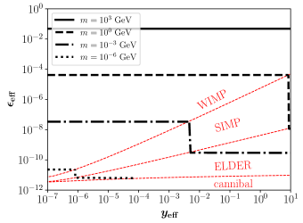
Figure 6: Parameter space that fits the observed DM relic abundance, for a production after reheating (that is, during the radiation-dominated era) for different DM masses. The same as in Fig. 2 but projected in the parameter space $[y_{\text{eff}},\,\epsilon_{\text{eff}}]$.

5.2 During Reheating

Alternatively, for a DM decoupling during reheating, Fig. 7 shows the parameter space that fits the entire observed abundance of DM assuming $\omega=0$ and $\alpha=3/8$, with $x_{\text{rh}}=0.2$ (top left), $x_{\text{rh}}=5$ (top right), or $x_{\text{rh}}=60$ (bottom). It compares to Fig. 6 but for different low-temperature reheating scenarios, and corresponds to the information in the left panels of Fig. 5 projected in the plane $[y_{\text{eff}},\,\epsilon_{\text{eff}}]$.

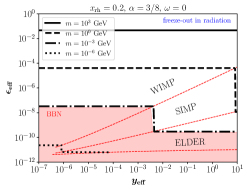
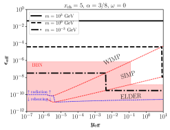
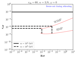
Figure 7: Parameter space that fits the observed DM relic abundance, for $\omega=0$ and $\alpha=3/8$. The different panels correspond to $x_{\text{rh}}=0.2$, 5 and 60. The same as in the left panels of Fig. 5 but projected in the parameter space $[y_{\text{eff}},\,\epsilon_{\text{eff}}]$. In the top-left panel the DM production always occurs during the radiation-dominated era, while in the lower panel, during reheating. However, in the top right panel, it can happen in the two regimes, depending on the DM mass. The transition between the two regimes is shown with a dashed blue line. The red bands are in tension with BBN.

As a first comment, we note that, as expected from Fig. 6, here the cannibal solution cannot be realized either. In fact, following the same procedure as in the previous section, the minimal value $x_{\text{k}}^{\text{min}}$ of $x_{\text{k}}$ required to have kinetic equilibrium between the two sectors is implicitly defined by

$$2x_{\text{k}}^{\text{min}}\,K_{1}^{2}(x_{\text{k}}^{\text{min}})+\left[1+\frac{3(1+\omega)}{2\alpha}\right]K_{1}(x_{\text{k}}^{\text{min}})\,K_{2}(x_{\text{k}}^{\text{min}})$$

$$\qquad\qquad\qquad=x_{\text{k}}^{\text{min}}\,K_{2}(x_{\text{k}}^{\text{min}})\left[K_{0}(x_{\text{k}}^{\text{min}})+K_{2}(x_{\text{k}}^{\text{min}})\right],$$ (5.9)

during reheating. We note that if $x_{\text{k}}^{\text{min}}$ is higher than $x_{\text{rh}}$, Eq. (5.2) ceases to be valid and therefore $x_{\text{k}}^{\text{min}}=x_{\text{rh}}$. Furthermore, the lower bound $\frac{3(1+\omega)}{2\alpha}\geq 2$, coming from a viable reheating (cf. Eq. (2.4)) implies that $x_{\text{k}}^{\text{min}}\gtrsim 1.8$ as in the case of radiation domination; cf. Eq. (5.8). We emphasize that, as $x_{\text{k}}>1$, the cannibal solution cannot be realized in this particle-physics scenario. Moreover, in addition to cannibals, the minimal value of $x_{\text{k}}$ also limits ELDERs. In fact, the ELDER solution during reheating requires that $x_{\text{k}}<x_{\text{rh}}$, and that is only possible in the range $2\leq\frac{3(1+\omega)}{2\alpha}<3$.

The left panel of Fig. 8 shows an example of the value of $x_{\text{k}}^{\text{min}}$ (black thick line) as a function of $\frac{3(1+\omega)}{2\alpha}$ for $x_{\text{rh}}=15$. The black dotted lines correspond to the solution of Eq. (5.2) and to $x_{\text{k}}^{\text{min}}=x_{\text{rh}}$. Here again, as a result of the choice of the interaction between the visible and dark sectors, the cannibal mechanism cannot be realized, even during reheating, as $x_{\text{k}}$ can never be smaller than 1. We emphasize that the previous conclusion is valid for any reheating scenario (any value of $\omega$, $\alpha$ and $T_{\text{rh}}$). Also, it is interesting to note that for this reheating scenario the ELDER solution cannot occur during reheating; it can happen, however, in the radiation-dominated era, as shown in the top panels of Fig. 7. In the top-left panel the DM freeze-out always occurs during the radiation-dominated era, whereas in the lower panel the DM freeze-out occurs during reheating. However, in the top right panel, it can happen in the two regimes, depending on the DM mass. The transition between the two regimes is shown with a dashed blue line.

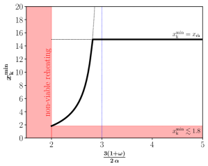
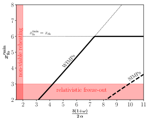
Figure 8: Left: Example of the minimal value $x_{\text{k}}^{\text{min}}$ of $x_{\text{k}}$ to have kinetic equilibrium between the dark and visible sectors during reheating (black thick line) for $x_{\text{rh}}=15$. Right: Example of the minimal value ${x^{\prime\text{min}}_{\text{fo}}}$ of ${x^{\prime}_{\text{fo}}}$ to have a chemical equilibrium (black thick lines) for $x_{\text{rh}}=6$. The solid line corresponds to WIMPs, while the dashed line corresponds to SIMPs. For $\frac{3(1+\omega)}{2\alpha}<2$ the reheating is not viable, while for ${x^{\prime}_{\text{fo}}}<3$ freeze out is relativistic (red bands).

In the top-left panel of Fig. 7 ($x_{\text{rh}}=0.2$), the DM freeze-out occurs in the radiation-dominated era, and therefore the curves coincide with those of Fig. 6. However, $x_{\text{rh}}$ could correspond to a sufficiently small value of $T_{\text{rh}}$ that rules out masses smaller than $m\lesssim 8\times 10^{-4}$ GeV due to the BBN constraint (red area). Even higher DM masses are in tension with BBN for higher values of $x_{\text{rh}}$, as seen in the top right panel ($x_{\text{rh}}=5$), where $m\gtrsim 2\times 10^{-2}$ GeV. Furthermore, the solution for $m=10^{-6}$ GeV is not viable, as it is smaller than the minimum mass $m\gtrsim 3\times 10^{-6}$ GeV for which chemical equilibrium is granted.

It is important to note that, in the two top panels of Fig. 7, only one of the two branches appearing in Fig. 5 (the one with higher values of ${x^{\prime}_{\text{fo}}}$) can be realized. Interestingly, for even larger values of $x_{\text{rh}}$ (that is, small reheating temperatures), the two branches can occur, as seen in the lower panel of Fig. 7 ($x_{\text{rh}}=60$). For a given mass, two disconnected solutions for WIMPs and two for SIMPs are realized for different values of the corresponding couplings. In addition, masses $m=10^{-6}$ GeV and $m=10^{-3}$ GeV cannot be generated, and the BBN bound disappears because large masses correspond to large reheating temperatures.

Concerning the possibility of the two solutions, recall that the first branch corresponds to values of ${x^{\prime}_{\text{fo}}}$ smaller than $x_{\text{fo}}^{\text{c}}$, as defined in Eq. (4.4). However, the existence of the first branch is challenged by the requirement of chemical equilibrium. Taking into account that ${x^{\prime}_{\text{fo}}}$ is defined by the equality $H({x^{\prime}_{\text{fo}}})=\Gamma_{2\to 2}({x^{\prime}_{\text{fo}}})$ for WIMPs and $H({x^{\prime}_{\text{fo}}})=\Gamma_{3\to 2}({x^{\prime}_{\text{fo}}})$ for SIMPs, the minimal value ${x^{\prime\text{min}}_{\text{fo}}}$ of ${x^{\prime}_{\text{fo}}}$ is implicitly defined as

$${x^{\prime\text{min}}_{\text{fo}}}\,K_{1}({x^{\prime\text{min}}_{\text{fo}}})+\left[3-\beta\,\frac{3(1+\omega)}{2\alpha}\right]K_{2}({x^{\prime\text{min}}_{\text{fo}}})=0\,,$$ (5.10)

with $\beta=1$ for WIMPs and $\beta=1/2$ for SIMPs. The right panel of Fig. 8 shows an example of ${x^{\prime\text{min}}_{\text{fo}}}$ for WIMPs (solid black line) and SIMPs (dashed black line), as a function of $\frac{3(1+\omega)}{2\alpha}$ assuming $x_{\text{rh}}=6$. For choice made in Fig. 7 ($\omega=0$ and $\alpha=3/8$), $\frac{3(1+\omega)}{2\alpha}=4$ and therefore ${x^{\prime\text{min}}_{\text{fo}}}\simeq 2.8$. We emphasize that even if the first branch is, in general, difficult to realize, it is not impossible to have it. As a sanity cross check, in Appendix A a complete numerical calculation was performed, solving the system of Boltzmann equations for the inflaton and SM radiation energy densities and the DM number density. Oscillations at the bottom of a quadratic potential and a constant decay width for the inflaton were assumed, which corresponds to $\omega=0$ and $\alpha=3/8$. An example of a point for which the two branches is explicitly shown.

In Fig. 7, corresponding to $\omega=0$ and $\alpha=3/8$, the ELDER solution cannot be realized during reheating, as $\frac{3(1+\omega)}{2\alpha}>3$. However, it can occur in the range $2\leq\frac{3(1+\omega)}{2\alpha}<3$. For example, Fig. 9 shows the parameter space that fits the observed DM relic abundance for $\omega=0$, $\alpha=3/4$ and $x_{\text{rh}}=200$. Here, the ELDER solution is clearly realized (and compatible with BBN) for DM masses above the GeV scale.

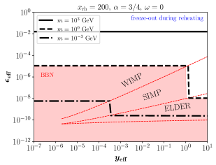
Figure 9: Parameter space that fits the observed DM relic abundance, for $\omega=0$, $\alpha=3/4$, and $x_{\text{rh}}=200$. The red band is in tension with BBN. Here, DM production always occurs during reheating.

In the following subsections, the three viable DM production mechanisms for this given particle-physics scenario will be analyzed in detail.

5.2.1 WIMPs

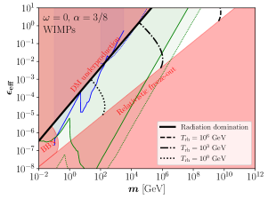
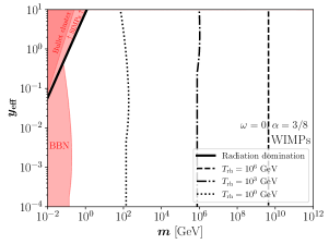
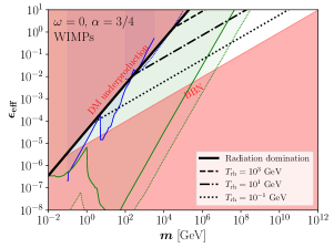
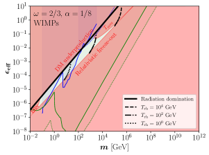
Figure 10: WIMPs. Top left and bottom: Parameter space $[m,\,\epsilon_{\text{eff}}]$ required to fit the observed DM relic abundance for $\omega=0$ and $\alpha=3/8$ (top left), $\omega=0$ and $\alpha=3/4$ (bottom left), and $\omega=2/3$ and $\alpha=1/8$ (bottom right), with different reheating temperatures. Top right: Allowed range of $y_{\text{eff}}$ values required to guarantee a WIMP solution, for $\omega=0$ and $\alpha=3/8$. The red bands are excluded because of DM underproduction, BBN, relativistic DM freeze-out, the maximum temperature of the SM bath, Bullet cluster, or the SIMP solution. The blue and green regions correspond to bounds (solid borders) or projections (dotted borders) from DM indirect and direct detection, respectively.

In addition to the broad parameter-space scans shown in Fig. 7, one can also perform a specific analysis for the different production mechanisms. The top left and the lower panels of Fig. 10 show the values of $\epsilon_{\text{eff}}$ required to fit the entire observed abundance of WIMP DM for different reheating temperatures. The thick black lines correspond to the usual high-temperature reheating scenario, where DM freezes out in the radiation-dominated era. As expected, the perturbativity bound on $\epsilon_{\text{eff}}$ restricts the WIMPs to be lighter than $\sim 130$ TeV [4]. Higher couplings produce a later chemical decoupling and, therefore, a DM underabundance. However, smaller couplings and larger masses can be explored in low-reheating scenarios because of the injection of entropy. In the case of $\omega=0$ and $\alpha=3/8$ (top left panel), the maximum WIMP mass is $m\sim\mathcal{O}(10^{11})$ GeV [65, 86, 88, 133], and is limited by perturbativity ($\epsilon_{\text{eff}}\lesssim 10$) and the condition of having a non-relativistic freeze-out (${x^{\prime}_{\text{fo}}}>3$). In other cosmological scenarios, for example, if $\omega=0$ and $\alpha=3/4$ (bottom left panel), DM can reach up to $m\sim\mathcal{O}(10^{12})$ GeV and this time it is bounded by perturbativity and the BBN limit on $T_{\text{rh}}$. A different scenario occurs for small values of $\alpha$. We remind unsuspecting readers that the parameter $\alpha$ controls the slope to the SM temperature during reheating (cf. Eq. (2.2)), and therefore small values of $\alpha$ imply a small separation between $T_{\text{rh}}$ and $T_{\text{max}}$. This is a potential issue, as DM to be a thermal relic must have a mass $m<T_{\text{max}}$. In Appendix B a detailed derivation of the maximal temperature $T_{\text{max}}$ reached by the thermal bath is presented. That bound is shown in the bottom right panel of Fig. 10, for $\omega=2/3$ and $\alpha=1/8$. In this particular case, the upper bound on the DM mass is $m\sim\mathcal{O}(10^{6})$ GeV.

WIMP solutions require the dominance of DM annihilation into SM particles over DM self-annihilation. This can be guaranteed if the self-coupling interaction rate $\Gamma_{3\to 2}$ is sufficiently suppressed. The top right panel of Fig. 10 shows the maximal allowed value for $y_{\text{eff}}$ to have a WIMP solution. For higher values of $y_{\text{eff}}$, the self-annihilation interaction rates of DM dominate, rendering DM a SIMP relic. Interestingly, beyond $\mathcal{O}$(1) MeV, $y_{\text{eff}}$ could be arbitrarily large (within the perturbative range) and still have a subdominant interaction rate. This is due to the strong Boltzmann suppression factor in the equilibrium DM number density.

We comment on some present and future possibilities of testing the current scenario using the different channels offered by DM indirect detection experiments. In Fig. 10 we overlay in blue (solid lines) present constraints coming from: $i)$ CMB spectral distortions from WIMP annihilation into charged particles [134], $ii)$ the combined analysis of $\gamma$-ray data using Fermi-LAT, HAWC, H.E.S.S., MAGIC, and VERITAS [135], and $iii)$ AMS-02 measurements of antimatter in cosmic rays, in the positron [136] and the antiproton [137] channels. Additionally, Fig. 10 also shows with blue dotted lines the projected sensitivity of the ground-based CTA experiment, which could be capable of testing WIMP DM at the TeV scale and above [145]. Assuming that the DM is coupled to all SM particles with the same contact interaction defined by Eq. (5.1), direct detection bounds from the elastic scattering of the DM with both electrons and nucleons become important and are shown by the shaded light green region (solid lines). The sub-GeV DM masses are constrained by the DM-electron elastic scattering, where the most stringent bounds come from XENON10, XENON100 [146] and DarkSide-50 [147]. Higher DM masses are constrained by bounds from DM-nucleon elastic scattering probes; the most stringent being DarkSide-50 [148], XENON1T [149] and LZ [150]. The future projected sensitivities are indicated by the dotted light-green line, where the maximum reach for DM-electron scattering can be achieved by DAMIC and SuperCDMS [151], while DARWIN [152], ARGO and DarkSide-20k [153] can attain the maximum reach for DM-nucleon scattering. It is interesting to note that actual direct and indirect DM detection experiments are already probing regions of parameter space where DM is produced deep in the reheating era. In particular, the scenario presented in the bottom right plot of Fig. 10 is completely ruled out. Finally, we also note that, as expected, all direct and indirect bounds and projections are the same in all panels of Fig. 10, because they depend only on the local details of the DM and not on its cosmological evolution.

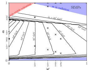
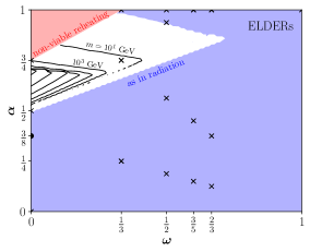
Figure 11: Contours for the maximal DM mass that can be produced by the different mechanisms: WIMP from $10^{6}$ GeV until $10^{14}$ GeV (top), SIMP from $10^{1}$ GeV until $10^{13}$ GeV (bottom left) and ELDER from $10^{1}$ GeV until $10^{13}$ GeV (bottom right). In the blue areas the maximal DM mass is the same as in radiation era, while in the red bands reheating is not viable.

A complete analysis of the maximal mass that can be produced by the WIMP mechanism compatible with all constraints is shown in the top panel of Fig. 11, using the same parameter space presented in Fig. 1. In particular, we ensure that $T_{\text{rh}}>T_{\text{bbn}}$, ${x^{\prime}_{\text{fo}}}>3$, $m<T_{\text{max}}$, $\epsilon_{\text{eff}}<10$, and $x_{\text{k}}>{x^{\prime}_{\text{fo}}}$. In the figure, the contours show three behaviors: $i)$ For $0.7\lesssim\alpha<1$, the maximal mass is set by the combination of perturbativity and BBN (cf. left bottom panel of Fig. 10), $ii)$ for $0.15\lesssim\alpha\lesssim 0.7$, it comes from perturbativity and ${x^{\prime}_{\text{fo}}}>3$ (cf. top panel of Fig. 10), while $iii)$ for $0<\alpha\lesssim 0.15$ from $T_{\text{max}}$ (cf. right bottom panel of Fig. 10). The maximum WIMP mass is $m\simeq 5\times 10^{14}$ GeV and occurs near $\omega\simeq 0$ and $\alpha\simeq 0.7$. Finally, we note that in the blue area the maximum DM mass is the same as in radiation domination.

5.2.2 SIMPs

In the left panel of Fig. 12, the parameter space that accounts for the entire observed abundance of DM through the SIMP mechanism is depicted with thick black lines for various reheating temperatures, assuming $\omega=0$ and $\alpha=3/8$. It compares to Fig. 10 but for the SIMP scenario. The solid black line represents the conventional high-temperature reheating scenario, where DM undergoes a chemical freeze-out through 3-to-2 annihilations during the radiation-dominated epoch. As anticipated, the perturbativity constraint on the coupling limits the SIMP DM to masses below approximately $\sim\mathcal{O}(1)$ GeV. Larger couplings result in delayed chemical decoupling, leading to a DM underabundance. Conversely, smaller couplings and larger masses can be investigated in low-reheating scenarios because of the entropy injection. It is interesting to note that in this case, SIMP DM can be as heavy as $\sim\mathcal{O}(10^{9})$ GeV with perturbative couplings, being limited by the requirement of a non-relativistic freeze-out. Additionally, light DM particles below the GeV ballpark, with sizable self-interactions, are in conflict with Bullet cluster data.

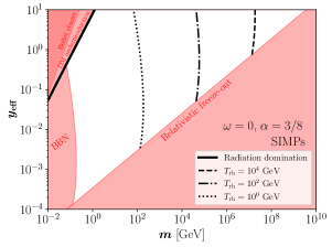
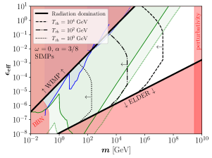
Figure 12: SIMPs. Left: Parameter space $[m,\,y_{\text{eff}}]$ that fits the observed DM relic abundance for $\omega=0$ and $\alpha=3/8$ and different reheating temperatures. Right: Maximal and minimal values of $\epsilon_{\text{eff}}$ required to have a SIMP solution. The red bands are excluded because of DM underproduction, BBN, relativistic DM freeze-out, or data from the Bullet cluster. The blue and green regions correspond to bounds (solid borders) or projections (dotted borders) from DM indirect and direct detection, respectively.

Even if the abundance of SIMP DM is fixed by the self-scattering coupling $y_{\text{eff}}$, there are consistency bounds on the interaction of the DM with the SM from above and below: too large values for $\epsilon_{\text{eff}}$ could make the DM a WIMP, while too small values for $\epsilon_{\text{eff}}$ could make it an ELDER (cf. Fig. 7). The right panel of Fig. 12 shows the interval in which $\epsilon_{\text{eff}}$ can vary while being compatible with a SIMP solution. Interestingly, for low-temperature reheating, such a range shrinks. Furthermore, the red vertical band on the right panel corresponds to the maximal mass allowed by perturbativity on the $y_{\text{eff}}$ coupling. Finally, we also overlay direct and indirect bounds and projections in the parameter space $[m,\,\epsilon_{\text{eff}}]$. It can be seen that a large fraction of the parameter space favored by low-temperature reheating is already in tension, especially with DM direct detection data, and even a larger fraction could be probed in next-generation experiments.

It is important to warn the reader that the apparent overlap of the parameter space for WIMPs and SIMPs in Figs. 10 and 12 is just an artifact of the projection of the full 4-dimensional parameter space ($m$, $\epsilon_{\text{eff}}$, $y_{\text{eff}}$ and $T_{\text{rh}}$) in the 2-dimensional planes $[m,\,y_{\text{eff}}]$ and $[m,\,\epsilon_{\text{eff}}]$.

The lower left panel of Fig. 11 shows the contours of the maximal SIMP DM mass that can be produced in a low-temperature reheating scenario. The behavior of these curves resembles the one in the WIMP case (cf. the top panel of Fig. 11). The contours show again three behaviors: $i)$ For $0.7\lesssim\alpha<1$, the maximal mass is set by the combination of perturbativity and BBN, $ii)$ for $0.15\lesssim\alpha\lesssim 0.7$, it comes from perturbativity and ${x^{\prime}_{\text{fo}}}>3$, while $iii)$ for $0<\alpha\lesssim 0.15$ from $T_{\text{max}}$. The maximum SIMP mass is $m\simeq 3\times 10^{13}$ GeV and occurs near $\omega\simeq 0$ and $\alpha\simeq 0.7$. Finally, we note that in the blue area the maximum DM mass is the same as in radiation domination.

5.2.3 ELDERs

The left panel of Fig. 13 shows the required values of $\epsilon_{\text{eff}}$ to fit the entire observed abundance of DM, for the ELDER mechanism, with different reheating temperatures, and assuming $\omega=1/3$ and $\alpha=3/4$. Even during the radiation-dominated era, it is expected that for a single DM mass a range of $\epsilon_{\text{eff}}$ is viable. However, the mass dependence is logarithmic and, de facto, the range collapses to a single point; cf. Fig. 6. Furthermore, and as expected from the top right panel of Fig. 12, a low-temperature reheating allows exploration of larger values for $\epsilon_{\text{eff}}$. Direct detection bounds rule out a large part of the parameter space, and future experiments can probe the allowed regions almost entirely. The right panel of Fig. 13 shows the minimal value of the self-coupling $y_{\text{eff}}$ compatible with the ELDER solution; smaller values would give rise to a WIMP. In radiation domination, the perturbative bound of $y_{\text{eff}}$ limits the DM mass to be below the GeV ballpark. For MeV DM masses, the Bullet cluster limits high values of the coupling. However, small couplings become viable for low-temperature reheating scenarios, increasing the DM mass window to $m\simeq 20$ GeV.

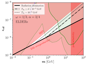
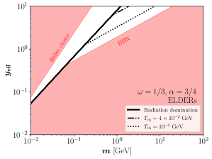
Figure 13: ELDERs. Left: Parameter space that fits the observed DM relic abundance, for $\omega=1/3$, $\alpha=3/4$ and different reheating temperatures. Right: Minimal coupling $y_{\text{eff}}$ compatible with the ELDER solution. The red bands are excluded because of DM overproduction, BBN or data from the Bullet cluster. The blue and green regions correspond to bounds (solid borders) or projections (dotted borders) from DM indirect and direct detection, respectively.

Finally, the lower right panel of Fig. 11 shows the contours of the maximal ELDER mass that can be produced. The curves are basically the same as in the SIMP case (cf. the lower left panel of Fig. 11), with the big difference that, to have a DM genesis in the low-temperature reheating era, one has to guarantee that $\frac{3(1+\omega)}{2\alpha}<3$; cf. the left panel of Fig. 8. For higher values, the ELDER solution can naturally take place, but DM is produced in the radiation-dominated era, which explains the size of the blue area. As in the case of SIMPs, the maximum ELDER mass is $m\simeq 3\times 10^{13}$ GeV and occurs near $\omega\simeq 0$ and $\alpha\simeq 0.7$.

6 Conclusions

Despite extensive experimental efforts during the last few decades, the nature of dark matter (DM) continues to be a mystery. Specifically, the hypothesis that DM consists of weakly interacting massive particles (WIMPs) that achieve thermal equilibrium with the standard model (SM) degrees of freedom has garnered substantial theoretical and experimental interest. However, no definitive evidence has emerged to support the existence of WIMP DM. This lack of conclusive results has led to the exploration of other mechanisms. On the thermal side, alternative production mechanisms exist; DM could be a strongly interacting massive particle (SIMP), an ELastically DEcoupling Relic (ELDER) or a cannibal. In these new paradigms, self-interactions within the DM sector play a crucial role in determining the abundance of DM. The key differences lie in the timing of chemical and kinetic freeze-out. For SIMPs, chemical freeze-out occurs while kinetic equilibrium is maintained, similar to that of WIMPs. In contrast, for ELDERs and cannibals, chemical freeze-out occurs after kinetic equilibrium is broken, with the latter occurring while the DM is non-relativistic or relativistic, respectively.

It is crucial to understand that the current abundance of DM is influenced not just by particle-physics dynamics but also by the cosmological history of the Universe. Given that the early Universe’s evolution remains largely uncertain, the conventional assumption is a Universe primarily governed by SM radiation from the end of cosmological inflation up to matter-radiation equality, with a sudden cosmic reheating happening at a very high SM temperature. Here, this picture is not taken for granted. In fact, we allowed noninstantaneous reheating and analyzed its impact on the thermal genesis of the DM.

The focus of this study has been on understanding the viability and implications of these thermal DM candidates in low-reheating scenarios, with careful consideration of their kinetic and/or chemical decoupling. We have studied general reheating scenarios by parameterizing the equation of state of the inflaton during reheating and the dependence of the SM temperature with the scale factor of the Universe. For the standard case of thermal DM production after reheating, we obtained in a model-independent way the region of parameter space that fits the total observed DM abundance for each type of DM candidate. We have then shown how these regions are modified when DM production occurs during reheating and identified the regions in tension with cosmological and laboratory constraints. For the WIMP, SIMP and ELDER mechanisms and for a given cosmology, two solutions that fit the entire observed DM abundance can occur: one during reheating and the other during the radiation-dominated era, or even both during reheating, as shown in Fig. 5.

We subsequently studied the implications for a simple particle-physics model, assuming contact operators for DM self-interactions and DM interactions with SM states, focusing on DM production both after and during reheating. In both cases, cannibal solutions are not viable as a result of strong temperature suppression when the DM is relativistic. Moreover, in this specific realization, WIMP, SIMP, and ELDER solutions become further constrained from BBN, and the possibility of having hot DM. At the same time, low reheating temperatures render viable larger mass values for the DM mass, up to the $10^{14}$ GeV ballpark, well beyond the usual limit of $130$ TeV for WIMPs and a few MeVs for SIMPs and ELDERs; see Fig. 11. Additionally, broader ranges for coupling values are now feasible, expanding the parameter space compared to the DM genesis during radiation domination. We have also shown how current direct and indirect limits on DM constrain significant parts of the allowed parameter space even in low-temperature reheating scenarios. Finally, we showed that upcoming direct detection experiments will be able to probe a substantial part of the remaining parameter space currently allowed.

Appendix A Numerical Validation

In this appendix, we compare our analytical estimations with full numerical results. As an example, we consider the reheating scenario in which the inflaton $\phi$ oscillates in a quadratic potential while perturbatively decaying into SM particles with a total decay width $\Gamma$. The evolution of the inflaton and SM radiation energy densities can be tracked with the system of Boltzmann equations

$$\frac{d\rho_{\phi}}{dt}+3\,H\,\rho_{\phi} =-\Gamma\,\rho_{\phi}\,,$$ (A.1)

$$\frac{d\rho_{R}}{dt}+4\,H\,\rho_{R} =+\Gamma\,\rho_{\phi}\,,$$ (A.2)

where $H$ is given in Eq. (2.5). This case corresponds to $\omega=0$ and $\alpha=3/8$, as discussed in Section 2. The left panel of Fig. 14 shows the evolution of $\rho_{\phi}$ (blue) and $\rho_{R}$ (black) as a function of the scale factor $a$, while the right panel shows the corresponding evolution of the SM temperature $T$, assuming $H_{I}=3\times 10^{-3}$ GeV and $\Gamma=8\times 10^{-22}$ GeV. For comparison, we also show the analytical estimations from Section 2 with thin black and blue dotted lines, in very good agreement with the fully numerical solution.

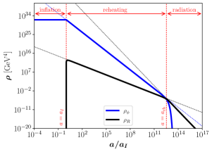
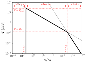
Figure 14: Left: Evolution of inflaton ($\rho_{\phi}$ in blue) and SM radiation ($\rho_{R}$ in black) energy densities as a function of the scale factor $a$. Right: Evolution of SM temperature $T$. In both plots, $H_{I}=3\times 10^{-3}$ GeV and $\Gamma=8\times 10^{-22}$ GeV were used. The thin black and blue dotted lines correspond to the analytical solution.

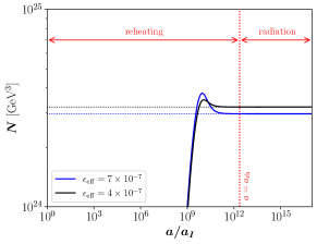
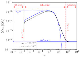
Figure 15: Evolution of the comoving number density $N$ (left) and the DM yield $Y$ (right), for $H_{I}=3\times 10^{-3}$ GeV, $\Gamma=8\times 10^{-22}$ GeV, $m=1$ GeV, $x_{\text{rh}}=43$ and $\epsilon_{\text{eff}}=4\times 10^{-7}$ (black) or $\epsilon_{\text{eff}}=7\times 10^{-7}$ (blue). The two benchmark points correspond to WIMP solutions and fit the entire observed DM abundance.

The evolution of the DM number density can be followed with the Boltzmann equation

$$\frac{dn}{dt}+3\,H\,n=-\langle\sigma v\rangle_{2\to 2}\left[n^{2}-n_{\text{eq}}^{2}\right],$$ (A.3)

that has to be solved in the background defined by Eqs. (A.1) and (A.2). As during reheating the SM entropy is not conserved, due to the decays of the inflaton into SM states, it is convenient to rewrite Eq. (A.3) as a function of the comoving number density $N\equiv n\,a^{3}$, which implies that

$$\frac{dN}{da}=-\frac{\langle\sigma v\rangle_{2\to 2}}{H\,a^{4}}\left[N^{2}-N_{\text{eq}}^{2}\right].$$ (A.4)

Figure 15 shows the fully numerical solution of $N$ (left) and the DM yield $Y$ (right), assuming $H_{I}=3\times 10^{-3}$ GeV, $\Gamma=8\times 10^{-22}$ GeV, $m=1$ GeV, $x_{\text{rh}}=43$ and two couplings: $\epsilon_{\text{eff}}=4\times 10^{-7}$ (black) or $\epsilon_{\text{eff}}=7\times 10^{-7}$ (blue). In the right panel, the DM yield at equilibrium is depicted with a blue dashed line, while the observed DM abundance is represented by a horizontal blue band. Several comments are in order: $i)$ Even if it is for a short period, DM reaches chemical equilibrium with the SM. That can be seen in the left panel, where $Y$ tracks the equilibrium yield, but also in the left panel, where the decrease in $N$ corresponds to the period in which chemical equilibrium is attained. As chemical equilibrium with the SM is reached, both solutions correspond to WIMPs. $ii)$ The two selected benchmark points fit the entire observed abundance of DM, as can be seen in the right panel. This is a clear example of the behavior already observed in Section 4, where, for a given mass, the abundance of WIMP DM can be fitted with two different values of the coupling. $iii)$ In general, this two-solution scenario is not easily realized, as it typically occurs on the verge of chemical equilibrium. If one solution occurs prior to chemical equilibrium, it would correspond to a (nonthermal) FIMP instead of a WIMP. In that case, for a given mass one would have two solutions: one WIMP and one FIMP [87]. $iv)$ We emphasize that this two-solution scenario can only be realized in the presence of a low-temperature reheating or, equivalently, in a nonstandard cosmological setup [154]. If chemical freeze-out occurs in a radiation-dominated era, the usual single solution takes place. And $v)$, the WIMP solution is typically realized with order-one couplings, if the freeze-out occurs in the radiation-dominated epoch. However, much smaller values such as $\epsilon_{\text{eff}}\sim\mathcal{O}(10^{-7})$ are needed if DM decouples during reheating, as in the present case.

For completeness, the evolution of the DM yield $Y$ as a function of the coupling $\epsilon_{\text{eff}}$ is shown in Fig. 16, for $H_{I}=3\times 10^{-3}$ GeV, $\Gamma=8\times 10^{-22}$ GeV, $m=1$ GeV and $x_{\text{rh}}=43$. The horizontal blue band corresponds to the observed abundance of DM that can be matched for the two values of the coupling mentioned above: $\epsilon_{\text{eff}}\simeq 4\times 10^{-7}$ and $\epsilon_{\text{eff}}\simeq 7\times 10^{-7}$. Between these two values, DM is overproduced, overclosing the Universe. We emphasize that for couplings close but smaller than $\epsilon_{\text{eff}}\simeq 4\times 10^{-7}$, chemical equilibrium is not granted, and therefore DM is no longer a thermal relic.

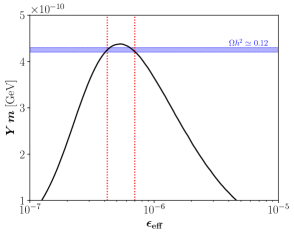
Figure 16: Evolution of DM yield $Y$ as a function of the coupling $\epsilon_{\text{eff}}$, for $H_{I}=3\times 10^{-3}$ GeV, $\Gamma=8\times 10^{-22}$ GeV, $m=1$ GeV and $x_{\text{rh}}=43$. The horizontal blue band corresponds to the observed abundance of DM that can be matched for two values of the coupling.

Appendix B Bound on $T_{\text{max}}$

During reheating, the energy densities of the inflaton and SM radiation can be written as

$$\rho_{\phi}(a) \simeq 3\,M_{P}^{2}\,H_{I}^{2}\left(\frac{a_{I}}{a}\right)^{3(1+\omega)},$$ (B.1)

$$\rho_{R}(a) \simeq\frac{\pi^{2}}{30}\,g_{\star}\,T_{\text{rh}}^{4}\left(\frac{a_{\text{rh}}}{a}\right)^{4\alpha},$$ (B.2)

where $a_{I}$ corresponds to the scale factor at the end of inflation and beginning of reheating, and $H_{I}\equiv H(a_{I})$ is the inflationary scale. The BICEP/Keck bound on the tensor-to-scalar ratio implies that $H_{I}\leq 2.0\times 10^{-5}~{}M_{P}$ [155]. Taking into account that at the end of reheating $\rho_{\phi}(a_{\text{rh}})=\rho_{R}(a_{\text{rh}})$, the maximal energy density reached by the SM thermal bath near $a=a_{I}$ can be estimated and therefore the maximal temperature $T_{\text{max}}$ is

$$T_{\text{max}}\simeq T_{\text{rh}}\left[\frac{90}{\pi^{2}\,g_{\star}}\,\frac{H_{I}^{2}\,M_{P}^{2}}{T_{\text{rh}}^{4}}\right]^{\frac{\alpha}{3(1+\omega)}}.$$ (B.3)

This limit on the maximum temperature reached by the SM bath is particularly relevant, as a thermally produced DM particle has to satisfy $m<T_{\text{max}}$.

References

- [1] Planck collaboration, Planck 2018 results. VI. Cosmological parameters, Astron. Astrophys. 641 (2020) A6 [1807.06209].
- [2] M. Cirelli, A. Strumia and J. Zupan, Dark Matter, 2406.01705.
- [3] G. Steigman, B. Dasgupta and J.F. Beacom, Precise Relic WIMP Abundance and its Impact on Searches for Dark Matter Annihilation, Phys. Rev. D 86 (2012) 023506 [1204.3622].
- [4] B.W. Lee and S. Weinberg, Cosmological Lower Bound on Heavy Neutrino Masses, Phys. Rev. Lett. 39 (1977) 165.
- [5] K. Griest and D. Seckel, Three exceptions in the calculation of relic abundances, Phys. Rev. D 43 (1991) 3191.
- [6] T. Hambye, Hidden vector dark matter, JHEP 01 (2009) 028 [0811.0172].
- [7] T. Hambye and M.H.G. Tytgat, Confined hidden vector dark matter, Phys. Lett. B 683 (2010) 39 [0907.1007].
- [8] F. D’Eramo and J. Thaler, Semi-annihilation of Dark Matter, JHEP 06 (2010) 109 [1003.5912].
- [9] G. Bélanger, K. Kannike, A. Pukhov and M. Raidal, Scalar Singlet Dark Matter, JCAP 01 (2013) 022 [1211.1014].
- [10] G. Bélanger, K. Kannike, A. Pukhov and M. Raidal, Minimal semi-annihilating scalar dark matter, JCAP 06 (2014) 021 [1403.4960].
- [11] G. Arcadi, M. Dutra, P. Ghosh, M. Lindner, Y. Mambrini, M. Pierre et al., The waning of the WIMP? A review of models, searches, and constraints, Eur. Phys. J. C 78 (2018) 203 [1703.07364].
- [12] L. Roszkowski, E.M. Sessolo and S. Trojanowski, WIMP dark matter candidates and searches - current status and future prospects, Rept. Prog. Phys. 81 (2018) 066201 [1707.06277].
- [13] G. Arcadi, D. Cabo-Almeida, M. Dutra, P. Ghosh, M. Lindner, Y. Mambrini et al., The Waning of the WIMP: Endgame?, 2403.15860.
- [14] Y. Hochberg, E. Kuflik, T. Volansky and J.G. Wacker, Mechanism for Thermal Relic Dark Matter of Strongly Interacting Massive Particles, Phys. Rev. Lett. 113 (2014) 171301 [1402.5143].
- [15] S.-M. Choi and H.M. Lee, SIMP dark matter with gauged symmetry, JHEP 09 (2015) 063 [1505.00960].
- [16] N. Bernal, C. García-Cely and R. Rosenfeld, WIMP and SIMP Dark Matter from the Spontaneous Breaking of a Global Group, JCAP 04 (2015) 012 [1501.01973].
- [17] N. Bernal, C. García-Cely and R. Rosenfeld, WIMP and SIMP Dark Matter from a Global U(1) Breaking, Nucl. Part. Phys. Proc. 267-269 (2015) 353.
- [18] P. Ko and Y. Tang, Self-interacting scalar dark matter with local symmetry, JCAP 05 (2014) 047 [1402.6449].
- [19] S.-M. Choi, H.M. Lee and M.-S. Seo, Cosmic abundances of SIMP dark matter, JHEP 04 (2017) 154 [1702.07860].
- [20] X. Chu and C. García-Cely, Self-interacting Spin-2 Dark Matter, Phys. Rev. D 96 (2017) 103519 [1708.06764].
- [21] N. Bernal, X. Chu, C. García-Cely, T. Hambye and B. Zaldivar, Production Regimes for Self-Interacting Dark Matter, JCAP 03 (2016) 018 [1510.08063].
- [22] N. Yamanaka, S. Fujibayashi, S. Gongyo and H. Iida, Dark matter in the hidden gauge theory, 1411.2172.
- [23] Y. Hochberg, E. Kuflik, H. Murayama, T. Volansky and J.G. Wacker, Model for Thermal Relic Dark Matter of Strongly Interacting Massive Particles, Phys. Rev. Lett. 115 (2015) 021301 [1411.3727].
- [24] H.M. Lee and M.-S. Seo, Communication with SIMP dark mesons via Z’-portal, Phys. Lett. B 748 (2015) 316 [1504.00745].
- [25] M. Hansen, K. Langæble and F. Sannino, SIMP model at NNLO in chiral perturbation theory, Phys. Rev. D 92 (2015) 075036 [1507.01590].
- [26] N. Bernal and X. Chu, SIMP Dark Matter, JCAP 01 (2016) 006 [1510.08527].
- [27] M. Heikinheimo, T. Tenkanen, K. Tuominen and V. Vaskonen, Observational Constraints on Decoupled Hidden Sectors, Phys. Rev. D 94 (2016) 063506 [1604.02401].
- [28] N. Bernal, X. Chu and J. Pradler, Simply split strongly interacting massive particles, Phys. Rev. D 95 (2017) 115023 [1702.04906].
- [29] M. Heikinheimo, T. Tenkanen and K. Tuominen, WIMP miracle of the second kind, Phys. Rev. D 96 (2017) 023001 [1704.05359].
- [30] N. Bernal, A. Chatterjee and A. Paul, Non-thermal production of Dark Matter after Inflation, JCAP 12 (2018) 020 [1809.02338].
- [31] A.A. de Laix, R.J. Scherrer and R.K. Schaefer, Constraints of selfinteracting dark matter, Astrophys. J. 452 (1995) 495 [astro-ph/9502087].
- [32] E. Kuflik, M. Perelstein, N.R.-L. Lorier and Y.-D. Tsai, Elastically Decoupling Dark Matter, Phys. Rev. Lett. 116 (2016) 221302 [1512.04545].
- [33] E. Kuflik, M. Perelstein, N.R.-L. Lorier and Y.-D. Tsai, Phenomenology of ELDER Dark Matter, JHEP 08 (2017) 078 [1706.05381].
- [34] E.D. Carlson, M.E. Machacek and L.J. Hall, Self-interacting dark matter, Astrophys. J. 398 (1992) 43.
- [35] D. Pappadopulo, J.T. Ruderman and G. Trevisan, Dark matter freeze-out in a nonrelativistic sector, Phys. Rev. D 94 (2016) 035005 [1602.04219].
- [36] M. Farina, D. Pappadopulo, J.T. Ruderman and G. Trevisan, Phases of Cannibal Dark Matter, JHEP 12 (2016) 039 [1607.03108].
- [37] J. McDonald, Thermally generated gauge singlet scalars as selfinteracting dark matter, Phys. Rev. Lett. 88 (2002) 091304 [hep-ph/0106249].
- [38] K.-Y. Choi and L. Roszkowski, E-WIMPs, AIP Conf. Proc. 805 (2005) 30 [hep-ph/0511003].
- [39] A. Kusenko, Sterile neutrinos, dark matter, and the pulsar velocities in models with a Higgs singlet, Phys. Rev. Lett. 97 (2006) 241301 [hep-ph/0609081].
- [40] K. Petraki and A. Kusenko, Dark-matter sterile neutrinos in models with a gauge singlet in the Higgs sector, Phys. Rev. D 77 (2008) 065014 [0711.4646].
- [41] L.J. Hall, K. Jedamzik, J. March-Russell and S.M. West, Freeze-In Production of FIMP Dark Matter, JHEP 03 (2010) 080 [0911.1120].
- [42] F. Elahi, C. Kolda and J. Unwin, UltraViolet Freeze-in, JHEP 03 (2015) 048 [1410.6157].
- [43] N. Bernal, M. Heikinheimo, T. Tenkanen, K. Tuominen and V. Vaskonen, The Dawn of FIMP Dark Matter: A Review of Models and Constraints, Int. J. Mod. Phys. A 32 (2017) 1730023 [1706.07442].
- [44] R. Allahverdi et al., The First Three Seconds: a Review of Possible Expansion Histories of the Early Universe, Open J.Astrophys. 4 (2021) [2006.16182].
- [45] S. Sarkar, Big bang nucleosynthesis and physics beyond the standard model, Rept. Prog. Phys. 59 (1996) 1493 [hep-ph/9602260].
- [46] M. Kawasaki, K. Kohri and N. Sugiyama, MeV scale reheating temperature and thermalization of neutrino background, Phys. Rev. D 62 (2000) 023506 [astro-ph/0002127].
- [47] S. Hannestad, What is the lowest possible reheating temperature?, Phys. Rev. D 70 (2004) 043506 [astro-ph/0403291].
- [48] F. De Bernardis, L. Pagano and A. Melchiorri, New constraints on the reheating temperature of the universe after WMAP-5, Astropart. Phys. 30 (2008) 192.
- [49] P.F. de Salas, M. Lattanzi, G. Mangano, G. Miele, S. Pastor and O. Pisanti, Bounds on very low reheating scenarios after Planck, Phys. Rev. D 92 (2015) 123534 [1511.00672].
- [50] J.D. Barrow, Massive Particles as a Probe of the Early Universe, Nucl. Phys. B 208 (1982) 501.
- [51] M. Kamionkowski and M.S. Turner, Thermal Relics: Do we Know their Abundances?, Phys. Rev. D 42 (1990) 3310.
- [52] J. McDonald, WIMP Densities in Decaying Particle Dominated Cosmology, Phys. Rev. D 43 (1991) 1063.
- [53] P. Salati, Quintessence and the relic density of neutralinos, Phys. Lett. B 571 (2003) 121 [astro-ph/0207396].
- [54] N. Fornengo, A. Riotto and S. Scopel, Supersymmetric dark matter and the reheating temperature of the universe, Phys. Rev. D 67 (2003) 023514 [hep-ph/0208072].
- [55] D. Comelli, M. Pietroni and A. Riotto, Dark energy and dark matter, Phys. Lett. B 571 (2003) 115 [hep-ph/0302080].
- [56] F. Rosati, Quintessential enhancement of dark matter abundance, Phys. Lett. B 570 (2003) 5 [hep-ph/0302159].
- [57] C. Pallis, Massive particle decay and cold dark matter abundance, Astropart. Phys. 21 (2004) 689 [hep-ph/0402033].
- [58] G.B. Gelmini and P. Gondolo, Neutralino with the right cold dark matter abundance in (almost) any supersymmetric model, Phys. Rev. D 74 (2006) 023510 [hep-ph/0602230].
- [59] M. Drees, H. Iminniyaz and M. Kakizaki, Abundance of cosmological relics in low-temperature scenarios, Phys. Rev. D 73 (2006) 123502 [hep-ph/0603165].
- [60] G. Gelmini, P. Gondolo, A. Soldatenko and C.E. Yaguna, The Effect of a late decaying scalar on the neutralino relic density, Phys. Rev. D 74 (2006) 083514 [hep-ph/0605016].
- [61] A. Arbey and F. Mahmoudi, SUSY constraints from relic density: High sensitivity to pre-BBN expansion rate, Phys. Lett. B 669 (2008) 46 [0803.0741].
- [62] T. Cohen, D.E. Morrissey and A. Pierce, Changes in Dark Matter Properties After Freeze-Out, Phys. Rev. D 78 (2008) 111701 [0808.3994].
- [63] A. Arbey and F. Mahmoudi, SUSY Constraints, Relic Density, and Very Early Universe, JHEP 05 (2010) 051 [0906.0368].
- [64] L. Roszkowski, S. Trojanowski and K. Turzyński, Neutralino and gravitino dark matter with low reheating temperature, JHEP 11 (2014) 146 [1406.0012].
- [65] A. Berlin, D. Hooper and G. Krnjaic, PeV-Scale Dark Matter as a Thermal Relic of a Decoupled Sector, Phys. Lett. B 760 (2016) 106 [1602.08490].
- [66] A. Berlin, D. Hooper and G. Krnjaic, Thermal Dark Matter From A Highly Decoupled Sector, Phys. Rev. D 94 (2016) 095019 [1609.02555].
- [67] F. D’Eramo, N. Fernández and S. Profumo, When the Universe Expands Too Fast: Relentless Dark Matter, JCAP 05 (2017) 012 [1703.04793].
- [68] S. Hamdan and J. Unwin, Dark Matter Freeze-out During Matter Domination, Mod. Phys. Lett. A 33 (2018) 1850181 [1710.03758].
- [69] L. Visinelli, (Non-)thermal production of WIMPs during kination, Symmetry 10 (2018) 546 [1710.11006].
- [70] M. Drees and F. Hajkarim, Dark Matter Production in an Early Matter Dominated Era, JCAP 02 (2018) 057 [1711.05007].
- [71] E. Hardy, Higgs portal dark matter in non-standard cosmological histories, JHEP 06 (2018) 043 [1804.06783].
- [72] N. Bernal, C. Cosme, T. Tenkanen and V. Vaskonen, Scalar singlet dark matter in non-standard cosmologies, Eur. Phys. J. C 79 (2019) 30 [1806.11122].
- [73] M. Drees and F. Hajkarim, Neutralino Dark Matter in Scenarios with Early Matter Domination, JHEP 12 (2018) 042 [1808.05706].
- [74] A. Betancur and Ó. Zapata, Phenomenology of doublet-triplet fermionic dark matter in nonstandard cosmology and multicomponent dark sectors, Phys. Rev. D 98 (2018) 095003 [1809.04990].
- [75] C. Maldonado and J. Unwin, Establishing the Dark Matter Relic Density in an Era of Particle Decays, JCAP 06 (2019) 037 [1902.10746].
- [76] A. Poulin, Dark matter freeze-out in modified cosmological scenarios, Phys. Rev. D 100 (2019) 043022 [1905.03126].
- [77] P. Arias, N. Bernal, A. Herrera and C. Maldonado, Reconstructing Non-standard Cosmologies with Dark Matter, JCAP 10 (2019) 047 [1906.04183].
- [78] C. Han, Higgsino Dark Matter in a Non-Standard History of the Universe, Phys. Lett. B 798 (2019) 134997 [1907.09235].
- [79] P. Chanda, S. Hamdan and J. Unwin, Reviving and Higgs Mediated Dark Matter Models in Matter Dominated Freeze-out, JCAP 01 (2020) 034 [1911.02616].
- [80] G. Arcadi, S. Profumo, F.S. Queiroz and C. Siqueira, Right-handed Neutrino Dark Matter, Neutrino Masses, and non-Standard Cosmology in a 2HDM, JCAP 12 (2020) 030 [2007.07920].
- [81] D. Bhatia and S. Mukhopadhyay, Unitarity limits on thermal dark matter in (non-)standard cosmologies, JHEP 03 (2021) 133 [2010.09762].
- [82] B. Barman, P. Ghosh, F.S. Queiroz and A.K. Saha, Scalar multiplet dark matter in a fast expanding Universe: Resurrection of the desert region, Phys. Rev. D 104 (2021) 015040 [2101.10175].
- [83] A. Cheek, L. Heurtier, Y.F. Pérez-González and J. Turner, Primordial black hole evaporation and dark matter production. II. Interplay with the freeze-in or freeze-out mechanism, Phys. Rev. D 105 (2022) 015023 [2107.00016].
- [84] G. Arcadi, J.P. Neto, F.S. Queiroz and C. Siqueira, Roads for right-handed neutrino dark matter: Fast expansion, standard freeze-out, and early matter domination, Phys. Rev. D 105 (2022) 035016 [2108.11398].
- [85] N. Bernal and Ó. Zapata, Dark Matter in the Time of Primordial Black Holes, JCAP 03 (2021) 015 [2011.12306].
- [86] N. Bernal and Y. Xu, WIMPs during reheating, JCAP 12 (2022) 017 [2209.07546].
- [87] J. Silva-Malpartida, N. Bernal, J. Jones-Pérez and R.A. Lineros, From WIMPs to FIMPs with low reheating temperatures, JCAP 09 (2023) 015 [2306.14943].
- [88] N. Bernal, P. Konar and S. Show, Unitarity bound on dark matter in low-temperature reheating scenarios, Phys. Rev. D 109 (2024) 035018 [2311.01587].
- [89] G. Arcadi, Thermal and non-thermal DM production in non-Standard Cosmologies: a mini review, 2406.11042.
- [90] N. Bernal, C. Cosme and T. Tenkanen, Phenomenology of Self-Interacting Dark Matter in a Matter-Dominated Universe, Eur. Phys. J. C 79 (2019) 99 [1803.08064].
- [91] N. Bernal and Ó. Zapata, Self-interacting Dark Matter from Primordial Black Holes, JCAP 03 (2021) 007 [2010.09725].
- [92] B. Spokoiny, Deflationary universe scenario, Phys. Lett. B 315 (1993) 40 [gr-qc/9306008].
- [93] P.G. Ferreira and M. Joyce, Cosmology with a primordial scaling field, Phys. Rev. D 58 (1998) 023503 [astro-ph/9711102].
- [94] J. Khoury, B.A. Ovrut, P.J. Steinhardt and N. Turok, The Ekpyrotic universe: Colliding branes and the origin of the hot big bang, Phys. Rev. D 64 (2001) 123522 [hep-th/0103239].
- [95] J. Khoury, P.J. Steinhardt and N. Turok, Designing cyclic universe models, Phys. Rev. Lett. 92 (2004) 031302 [hep-th/0307132].
- [96] M. Gasperini and G. Veneziano, The Pre-big bang scenario in string cosmology, Phys. Rept. 373 (2003) 1 [hep-th/0207130].
- [97] J.K. Erickson, D.H. Wesley, P.J. Steinhardt and N. Turok, Kasner and mixmaster behavior in universes with equation of state , Phys. Rev. D 69 (2004) 063514 [hep-th/0312009].
- [98] J.D. Barrow and K. Yamamoto, Anisotropic Pressures at Ultra-stiff Singularities and the Stability of Cyclic Universes, Phys. Rev. D 82 (2010) 063516 [1004.4767].
- [99] A. Ijjas and P.J. Steinhardt, A new kind of cyclic universe, Phys. Lett. B 795 (2019) 666 [1904.08022].
- [100] R.J. Scherrer, How slowly can the early Universe expand?, Phys. Rev. D 106 (2022) 103516 [2209.03421].
- [101] M.S. Turner, Coherent Scalar Field Oscillations in an Expanding Universe, Phys. Rev. D 28 (1983) 1243.
- [102] K.D. Lozanov and M.A. Amin, Equation of State and Duration to Radiation Domination after Inflation, Phys. Rev. Lett. 119 (2017) 061301 [1608.01213].
- [103] K.D. Lozanov and M.A. Amin, Self-resonance after inflation: oscillons, transients and radiation domination, Phys. Rev. D 97 (2018) 023533 [1710.06851].
- [104] D. Bodeker, Moduli decay in the hot early Universe, JCAP 06 (2006) 027 [hep-ph/0605030].
- [105] K. Mukaida and K. Nakayama, Dynamics of oscillating scalar field in thermal environment, JCAP 01 (2013) 017 [1208.3399].
- [106] R. Daido, F. Takahashi and W. Yin, The ALP miracle: unified inflaton and dark matter, JCAP 05 (2017) 044 [1702.03284].
- [107] R.T. Co, E. González and K. Harigaya, Increasing Temperature toward the Completion of Reheating, JCAP 11 (2020) 038 [2007.04328].
- [108] M.A.G. García, K. Kaneta, Y. Mambrini and K.A. Olive, Inflaton Oscillations and Post-Inflationary Reheating, JCAP 04 (2021) 012 [2012.10756].
- [109] A. Ahmed, B. Grzadkowski and A. Socha, Implications of time-dependent inflaton decay on reheating and dark matter production, Phys. Lett. B 831 (2022) 137201 [2111.06065].
- [110] B. Barman, N. Bernal, Y. Xu and Ó. Zapata, Ultraviolet freeze-in with a time-dependent inflaton decay, JCAP 07 (2022) 019 [2202.12906].
- [111] A. Banerjee and D. Chowdhury, Fingerprints of freeze-in dark matter in an early matter-dominated era, SciPost Phys. 13 (2022) 022 [2204.03670].
- [112] P. Arias, N. Bernal, J.K. Osiński and L. Roszkowski, Dark matter axions in the early universe with a period of increasing temperature, JCAP 05 (2023) 028 [2207.07677].
- [113] R.T. Co and K. Harigaya, Gravitino Production Suppressed by Dynamics of Sgoldstino, JHEP 10 (2017) 207 [1707.08965].
- [114] C. Cosme, F. Costa and O. Lebedev, Temperature evolution in the Early Universe and freeze-in at stronger coupling, JCAP 06 (2024) 031 [2402.04743].
- [115] Y. Shtanov, J.H. Traschen and R.H. Brandenberger, Universe reheating after inflation, Phys. Rev. D 51 (1995) 5438 [hep-ph/9407247].
- [116] K. Ichikawa, T. Suyama, T. Takahashi and M. Yamaguchi, Primordial Curvature Fluctuation and Its Non-Gaussianity in Models with Modulated Reheating, Phys. Rev. D 78 (2008) 063545 [0807.3988].
- [117] N. Bernal, S. Cléry, Y. Mambrini and Y. Xu, Probing reheating with graviton bremsstrahlung, JCAP 01 (2024) 065 [2311.12694].
- [118] B. Barman, N. Bernal and Y. Xu, Resonant Reheating, 2404.16090.
- [119] G.F. Giudice, E.W. Kolb and A. Riotto, Largest temperature of the radiation era and its cosmological implications, Phys. Rev. D 64 (2001) 023508 [hep-ph/0005123].
- [120] M. Drees, F. Hajkarim and E.R. Schmitz, The Effects of QCD Equation of State on the Relic Density of WIMP Dark Matter, JCAP 06 (2015) 025 [1503.03513].
- [121] Particle Data Group collaboration, Review of Particle Physics, PTEP 2022 (2022) 083C01.
- [122] M. Viel, G.D. Becker, J.S. Bolton and M.G. Haehnelt, Warm dark matter as a solution to the small scale crisis: New constraints from high redshift Lyman- forest data, Phys. Rev. D 88 (2013) 043502 [1306.2314].
- [123] V. Iršič et al., New Constraints on the free-streaming of warm dark matter from intermediate and small scale Lyman- forest data, Phys. Rev. D 96 (2017) 023522 [1702.01764].
- [124] N. Sabti, J. Alvey, M. Escudero, M. Fairbairn and D. Blas, Refined Bounds on MeV-scale Thermal Dark Sectors from BBN and the CMB, JCAP 01 (2020) 004 [1910.01649].
- [125] N. Sabti, J. Alvey, M. Escudero, M. Fairbairn and D. Blas, Addendum: Refined bounds on MeV-scale thermal dark sectors from BBN and the CMB, JCAP 08 (2021) A01 [2107.11232].
- [126] D. Clowe, A. González and M. Markevitch, Weak lensing mass reconstruction of the interacting cluster 1E0657-558: Direct evidence for the existence of dark matter, Astrophys. J. 604 (2004) 596 [astro-ph/0312273].
- [127] M. Markevitch, A.H. González, D. Clowe, A. Vikhlinin, L. David, W. Forman et al., Direct constraints on the dark matter self-interaction cross-section from the merging galaxy cluster 1E0657-56, Astrophys. J. 606 (2004) 819 [astro-ph/0309303].
- [128] S.W. Randall, M. Markevitch, D. Clowe, A.H. González and M. Bradač, Constraints on the Self-Interaction Cross-Section of Dark Matter from Numerical Simulations of the Merging Galaxy Cluster 1E 0657-56, Astrophys. J. 679 (2008) 1173 [0704.0261].
- [129] D. Harvey, R. Massey, T. Kitching, A. Taylor and E. Tittley, The non-gravitational interactions of dark matter in colliding galaxy clusters, Science 347 (2015) 1462 [1503.07675].
- [130] K. Bondarenko, A. Boyarsky, T. Bringmann and A. Sokolenko, Constraining self-interacting dark matter with scaling laws of observed halo surface densities, JCAP 04 (2018) 049 [1712.06602].
- [131] D. Harvey, A. Robertson, R. Massey and I.G. McCarthy, Observable tests of self-interacting dark matter in galaxy clusters: BCG wobbles in a constant density core, Mon. Not. Roy. Astron. Soc. 488 (2019) 1572 [1812.06981].
- [132] K. Griest and M. Kamionkowski, Unitarity Limits on the Mass and Radius of Dark Matter Particles, Phys. Rev. Lett. 64 (1990) 615.
- [133] R. Coy, J. Kimus and M.H.G. Tytgat, Light from darkness: history of a hot dark sector, 2405.10792.
- [134] R.K. Leane, T.R. Slatyer, J.F. Beacom and K.C.Y. Ng, GeV-scale thermal WIMPs: Not even slightly ruled out, Phys. Rev. D 98 (2018) 023016 [1805.10305].
- [135] Hess, HAWC, VERITAS, MAGIC, H.E.S.S., Fermi-LAT collaboration, Combined dark matter searches towards dwarf spheroidal galaxies with Fermi-LAT, HAWC, H.E.S.S., MAGIC, and VERITAS, PoS ICRC2021 (2021) 528 [2108.13646].
- [136] L. Bergstrom, T. Bringmann, I. Cholis, D. Hooper and C. Weniger, New Limits on Dark Matter Annihilation from AMS Cosmic Ray Positron Data, Phys. Rev. Lett. 111 (2013) 171101 [1306.3983].
- [137] F. Calore, M. Cirelli, L. Derome, Y. Genolini, D. Maurin, P. Salati et al., AMS-02 antiprotons and dark matter: Trimmed hints and robust bounds, SciPost Phys. 12 (2022) 163 [2202.03076].
- [138] M. Zemp, J. Diemand, M. Kuhlen, P. Madau, B. Moore, D. Potter et al., The Graininess of Dark Matter Haloes, Mon. Not. Roy. Astron. Soc. 394 (2009) 641 [0812.2033].
- [139] M. Pato, O. Agertz, G. Bertone, B. Moore and R. Teyssier, Systematic uncertainties in the determination of the local dark matter density, Phys. Rev. D 82 (2010) 023531 [1006.1322].
- [140] N. Bernal, J.E. Forero-Romero, R. Garani and S. Palomares-Ruiz, Systematic uncertainties from halo asphericity in dark matter searches, JCAP 09 (2014) 004 [1405.6240].
- [141] M. Boudaud et al., A new look at the cosmic ray positron fraction, Astron. Astrophys. 575 (2015) A67 [1410.3799].
- [142] N. Bernal, J.E. Forero-Romero, R. Garani and S. Palomares-Ruiz, Systematic uncertainties from halo asphericity in dark matter searches, Nucl. Part. Phys. Proc. 267-269 (2015) 345.
- [143] N. Bernal, L. Necib and T.R. Slatyer, Spherical Cows in Dark Matter Indirect Detection, JCAP 12 (2016) 030 [1606.00433].
- [144] M. Benito, N. Bernal, N. Bozorgnia, F. Calore and F. Iocco, Particle Dark Matter Constraints: the Effect of Galactic Uncertainties, JCAP 02 (2017) 007 [1612.02010].
- [145] CTA collaboration, Sensitivity of the Cherenkov Telescope Array to a dark matter signal from the Galactic centre, JCAP 01 (2021) 057 [2007.16129].
- [146] R. Essig, T. Volansky and T.-T. Yu, New Constraints and Prospects for sub-GeV Dark Matter Scattering off Electrons in Xenon, Phys. Rev. D 96 (2017) 043017 [1703.00910].
- [147] DarkSide collaboration, Search for Dark Matter Particle Interactions with Electron Final States with DarkSide-50, Phys. Rev. Lett. 130 (2023) 101002 [2207.11968].
- [148] DarkSide-50 collaboration, Search for low-mass dark matter WIMPs with 12 ton-day exposure of DarkSide-50, Phys. Rev. D 107 (2023) 063001 [2207.11966].
- [149] XENON collaboration, First Dark Matter Search Results from the XENON1T Experiment, Phys. Rev. Lett. 119 (2017) 181301 [1705.06655].
- [150] LZ collaboration, First Dark Matter Search Results from the LUX-ZEPLIN (LZ) Experiment, Phys. Rev. Lett. 131 (2023) 041002 [2207.03764].
- [151] R. Essig, M. Fernandez-Serra, J. Mardon, A. Soto, T. Volansky and T.-T. Yu, Direct Detection of sub-GeV Dark Matter with Semiconductor Targets, JHEP 05 (2016) 046 [1509.01598].
- [152] DARWIN collaboration, DARWIN: towards the ultimate dark matter detector, JCAP 11 (2016) 017 [1606.07001].
- [153] J. Billard et al., Direct detection of dark matter—APPEC committee report*, Rept. Prog. Phys. 85 (2022) 056201 [2104.07634].
- [154] J. Silva-Malpartida, N. Bernal, J. Jones-Pérez and R.A. Lineros, From WIMPs to FIMPs in Nonstandard Cosmologies, 240*.soon.
- [155] BICEP, Keck collaboration, Improved Constraints on Primordial Gravitational Waves using Planck, WMAP, and BICEP/Keck Observations through the 2018 Observing Season, Phys. Rev. Lett. 127 (2021) 151301 [2110.00483].