Generalized Gibbs ensembles in weakly interacting dissipative systems and digital quantum computers

Abstract

Digital quantum computers promise to solve important and challenging problems in many-body quantum physics. However, at least for the superconducting platforms, their current limitation is the noise level. It thus seems more reasonable to presently use them to model dissipative systems, where platforms’ native noise is not that crucial. Here, we propose using a digital quantum computer to showcase the activation of integrability by realizing exotic generalized Gibbs ensembles in weakly dissipative integrable systems. Dissipation is realized by coupling system’s qubits to periodically reset ancilla ones, like in the protocol [1] recently used to realize dissipative cooling. We derive the effective equations of motion for trotterized dynamics and contrast such a setup to the usual Lindblad continuous evolution. For simplicity, we consider and compare different approaches to calculating steady-states of non-interacting integrable systems weakly coupled to baths, where thermodynamic results can be obtained via a generalized scattering theory between the Bogoliubov quasiparticles. Corresponding quantum computer implementation would illuminate the possibilities of realizing similar exotic states in nearly integrable quantum materials.

I Introduction

Most of the quantum simulators and computers strive to eliminate any elements of openness, however, to some extent, it is unavoidable: atom loss and dipolar coupling in cold atoms, light leakage in cavities, heating, dephasing and other errors on gates, etc. In the pioneering experiments with trapped ions [2] and also in some more recent experiments with superconducting qubit platform [1], there have been propositions on how to actually use engineered dissipation [3, 4] to prepare target/ground states [5, 6] or to measure phase transitions [7]. Such protocols might also be more resilient to the inherent platforms’ noise. For example, in a recent implementation of trotterized transverse field Ising model with the superconducting circuit [1], a dissipative cooling towards the ground state has been implemented by coupling the system’s qubits to ancilla ones that are periodically reset. This realization builds on a series of theoretical works [8, 9, 10, 11, 12, 13, 14, 15] proposing cooling in quantum computers by coupling to low entropy baths (ancilla qubits), involving tuning the Hamiltonian of the ancilla qubits and its coupling to the system qubits. While the above mentioned cooling protocols might be more naturally and efficiently implemented with an ergodic system [8], considering non-interacting models can assist to get more exact/analytical insight into the conditions required [16].

In many cases, non-interacting many-body models are the cornerstone of our understanding and description of many-body physics. The fact that they are exactly diagonalizable via the Bogoliubov transformation makes them also a rare and appealing platform to study non-equilibrium many-body physics [17, 18, 19]. In the context of thermalization or its failure, non-interacting systems are an example of models with extensively many conserved quantities [17, 18]. The conserved quantities of translationally invariant models are simply the mode occupation operators of Bogoliubov quasiparticles [18] and one can use those to construct extensively many local conserved quantities [17]. The existence of macroscopically many conserved quantities places non-interacting many-body systems on the same footing as more general interacting integrable systems, in the sense that they fail to thermalize due to the presence of additional conservation laws, or equivalently, limited quasiparticle scattering [18, 17, 19]. Non-interacting models have been among the first for which the applicability of generalized Gibbs ensembles (GGEs) [20] as a local description of steady states reached after a sudden quench has been demonstrated [21, 22, 23, 24, 25, 26, 27]. Introducing additional Lagrange parameters, associated with the mode occupation operators or the local conserved operators, proved to be a successful way to take into account constraints on equilibration. More recent studies showed that a GGE description applies not only to quenches in isolated models but also to weakly dissipative integrable systems, including the non-interacting ones [28, 29, 30, 31, 32, 33, 34, 35, 36, 37, 38, 39]. In that case, GGE gives the zeroth order approximation to the dynamics and the steady state density matrix. The main difference between the closed and open setup is that for the former, the Lagrange multipliers are determined by the post-quench state, while in the open setup, they are determined by the dissipation operator [28, 29, 30, 31, 32, 33]. Only if the dissipators obeys detailed balance condition, the stabilized steady-state is thermal [29, 16]. In any other situations, such weakly dissipative, nearly integrable systems tend to converge to highly non-thermal GGEs. This explains why a careful tuning of parameters is necessary for preparation of thermal states on a quantum computer modelling an integrable system [1, 16].

In this work, we marry the two topics and show that for generic weak couplings between integrable system and periodically reset ancilla qubits, highly non-thermal generalized Gibbs ensembles would be stabilized with quantum computers. We focus on the non-interacting integrable systems, for which we also review and compare different approaches to thermodynamically large systems. In Sec. II, description of weakly open integrable systems in terms of (time dependent) generalized Gibbs ensembles is introduced in general. In Sec. III, we first present time evolution in terms of GGEs in a traditional weakly dissipative continuous Lindblad model with transverse field Ising model coupled to Lindblad baths. We show how within the generalized Gibbs ensemble descriptions, equations of motion simplify into a generalized scattering problem between the Bogoliubov quasiparticles. In Sec. IV we highlight that superconducting circuit platforms [1] or digital trapped ion quantum computers [40] would be ideal implementations of all elements required to show that highly non-thermal and possibly exotic GGEs emerge in weakly open nearly integrable systems. We extend our formalism to such a Floquet time evolution with reset of ancilla qubits. To obtain equations of motion for the occupation of Bogoliubov quasiparticles, we derive the Lindblad master equation for a weakly dissipative trotterized setup. In the end, we propose how reviving of integrability can be detected via measurement of anomalously slow decay of certain spatial correlations. In a more technical Sec. V, different approaches to non-interacting weakly dissipative systems are compared. In Sec. VI, we conclude that an actual experimental realization would prove the concept of GGEs to be applicable also for other platforms and, ultimately, for nearly integrable materials [41, 42].

II Setup

We first review the structure of the density matrix perturbation theory using the example of a traditional Lindblad setup with a continuous model. In the next section, we generalize this to a trotterized implementation with a reset protocol relevant to digital quantum computers. Within the continuous implementations, we consider a system with dominant unitary dynamics described by a non-interacting translationally invariant Hamiltonian $H_{0}$, which has a diagonal form in terms of mode occupation operators $n_{q}$ of Bogoliubov quasiparticles,

$$H_{0}=\sum_{q}\varepsilon_{q}n_{q}+E_{0}$$ (1)

where $\varepsilon_{q}$ is the dispersion of a single particle excitation with momentum $q$ and $E_{0}$ is a constant shift in energy. In addition, the system is weakly coupled in bulk to baths described by the dissipator $\hat{\mathcal{D}}$,

$$\hat{\mathcal{L}}\rho=-i[H_{0},\rho]+\hat{\mathcal{D}}\rho,\ \hat{\mathcal{D}}\rho=\epsilon\sum_{i}L_{i}\rho L_{i}^{\dagger}-\frac{1}{2}\{L_{i}^{\dagger}L_{i},\rho\}.$$ (2)

Here, $\epsilon\ll 1$ is a weak coupling parameter, and $L_{i}$ are the Lindblad operators acting around site $i$.

In our previous works [28, 30, 31, 29], we showed that the zeroth order (in $\epsilon$) approximation to the steady state and the slow evolution towards the steady state has the form of a generalized Gibbs ensemble (GGE). For the non-interacting translationally invariant $H_{0}$ one can build a GGE using the local extensive conserved quantities $C_{i}$, $[H_{0},C_{i}]=0$, or the mode occupation operators $n_{q}$,

$$\rho_{\bm{\mu}}(t)=\frac{e^{-\sum_{q}\mu_{q}(t)n_{q}}}{\text{Tr}[e^{-\sum_{q}\mu_{q}(t)n_{q}}]}.$$ (3)

Here, $\mu_{q}$ are the associated Lagrange multipliers. Since the dissipator weakly breaks the integrability properties of $H_{0}$, mode occupations are slowly changing, in the lowest order described by the rate equations

$$\langle\dot{n}_{q}\rangle(t)\approx\text{Tr}\left[n_{q}\hat{\mathcal{D}}\frac{e^{-\sum_{q^{\prime}}\mu_{q^{\prime}}(t)n_{q^{\prime}}}}{\text{Tr}[e^{-\sum_{q^{\prime}}\mu_{q^{\prime}}(t)n_{q^{\prime}}}]}\right],$$ (4)

where contribution of order $\epsilon^{2}$ and higher are neglected. Equivalently, the Langrange multipliers $\mu_{q}$ will be changing on the timescale $\mathcal{O}(1/\epsilon)$ according to the following equation derived in Ref. [30],

$$\dot{\mu}_{q}(t)=-\sum_{q^{\prime}}(\chi^{-1})_{q,q^{\prime}}(t)\,\langle\dot{n}_{q^{\prime}}\rangle(t).$$ (5)

Here, $\chi_{q,q^{\prime}}(t)=\langle n_{q}n_{q^{\prime}}\rangle_{\rho_{\bm{\mu}(t)}}-\langle n_{q}\rangle_{\rho_{\bm{\mu}(t)}}\langle n_{q^{\prime}}\rangle_{\rho_{\bm{\mu}(t)}}$ is the $\{q,q^{\prime}\}$ entry of matrix $\chi$ and $\langle O\rangle_{\rho_{\bm{\mu}}}=\text{Tr}[O\rho_{\bm{\mu}}]$. In the case of free fermions, matrix $\chi$ is of a diagonal form $\chi_{q,q^{\prime}}(t)=\delta_{q,q^{\prime}}\,e^{-\mu_{q}(t)}/(1+e^{-\mu_{q}(t)})^{2}$.

We use Eq. (5) to perform time evolutions from simple thermal initial states in the following sections.

III Continuous Model

We consider the transverse field Ising model

$$H_{0}=\sum_{i}J\sigma^{x}_{i}\sigma^{x}_{i+1}+h\sigma^{z}_{i},$$ (6)

as a paradigmatic non-interacting integrable model, which can be (at least approximately) realized with quantum simulators [43, 44, 45, 46, 47, 48]. In order to obtain its mode occupation operators, we perform the Jordan-Wigner tranformation from spin-$\frac{1}{2}$ degrees of freedom to spinless fermions

$$\sigma_{j}^{z} =2c_{j}^{\dagger}c_{j}-1,\ \sigma_{j}^{+}=e^{i\pi\sum_{l<j}n_{j}}c_{j}^{\dagger},$$ (7)

and the Fourier transform from the positional basis to the momentum basis

$$c_{j} =\frac{e^{-i\pi/4}}{\sqrt{N}}\sum_{q}e^{iqj}c_{q}.$$ (8)

Finally, the Bogoliubov transformation

$$c_{q} =u_{q}d_{q}-v_{q}d_{-q}^{\dagger},$$ (9)

$$u_{q} =\frac{(\varepsilon_{q}+a_{q})}{\sqrt{2\varepsilon_{q}(\varepsilon_{q}+a_{q})}},\ v_{q}=\frac{b_{q}}{\sqrt{2\varepsilon_{q}(\varepsilon_{q}+a_{q})}},$$

$$a_{q} =2(J\cos{q}+h),\ b_{q}=2J\sin{q},$$

$$\epsilon_{q} =2\sqrt{J^{2}+2hJ\cos{q}+h^{2}},$$

brings the Hamiltonian into a diagonal form

$$H=\sum_{q}\varepsilon_{q}\left(n_{q}-\frac{1}{2}\right),\ n_{q}=d_{q}^{\dagger}d_{q}.$$ (10)

Therefore, the Hamiltonian and all the local conserved charges, $C_{i}=\sum_{q}\mathfrak{c}^{(i)}_{q}n_{q}$, can be expressed in terms of mode occupation operators. One should note that periodic boundary conditions in the spin picture are translated to periodic boundary conditions in the fermion picture for an odd number of particles and anti-periodic for an even number of particles. Consequently, the two cases are diagonalized by a different set of wave vectors, $\mathcal{K}^{+}=\{\frac{2\pi}{L}(q+\frac{1}{2}),q=0,\dots L-1\}$ for the even sector and $\mathcal{K}^{-}=\{\frac{2\pi}{L}q,q=0,\dots L-1\}$ for the odd sector. The two symmetry sectors are uncoupled by the Hamiltonian dynamics and should be treated separately.

As an example of coupling to baths, which stabilize a nontrivial steady state, we consider the following Lindblad operator

$$L_{j}=S_{j}^{+}S_{j+1}^{-}+S_{j}^{z}+\frac{1}{2}\mathbb{1}_{j}.$$ (11)

We choose an operator which after the Jordan-Wigner, Fourier and Bogoliubov transformations obtains a compact form without any string operators,

$$L_{j}=\sum_{q,q^{\prime}}\frac{e^{-ij(q-q^{\prime})}}{N}(1+e^{iq^{\prime}})(u_{q}d_{q}^{\dagger}-v_{q}d_{-q})(u_{q^{\prime}}d_{q^{\prime}}-v_{q^{\prime}}d_{-q^{\prime}}^{\dagger}).$$ (12)

However, due to the form of dissipator with $L_{i}$ and $L_{i}^{\dagger}$ pairs, Eq. (2), analysis is not much more complicated in the presence of string operators as well.

These Lindblad operators preserve the parity, i.e., some terms preserve the number of fermions while others change it by two. Therefore, we get two steady states, one for the even and one for the odd parity sector. Thermodynamically, the two solutions behave the same. We consider only the even sector in the following and work with momenta $\mathcal{K}^{+}$.

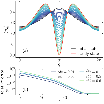
Figure 1: (a) Time evolution from an initial thermal mode occupation with $\beta=0.323$ to a highly non-thermal steady state distribution, stabilized by our choice of Lindblad operators, Eq. (12). (b) Relative error $\sum_{q}|(\langle n_{q}\rangle(t)-\langle n_{q}\rangle_{0}(t))/\langle n_{q}\rangle_{0}(t)|$ of the occupations $\langle n_{q}\rangle(t)$ obtained with Euler method with time steps $\epsilon\delta t=0.01,...,0.6$ and the reference $\langle n_{q}\rangle_{0}(t)$ evaluated with smallest $\epsilon\delta t=0.005$. At late times differences are tiny. Parameters: $J=1,h=0.6,L=10^{5}$.

To calculate the time evolution as described in Sec. II, the central object to be evaluated is the expression (4) for $\langle\dot{n}_{q}\rangle$, which can be split as

$$\langle\dot{n}_{q}\rangle=\epsilon\sum_{j}\langle L_{j}^{\dagger}n_{q}L_{j}\rangle-\langle n_{q}L_{j}^{\dagger}L_{j}\rangle$$ (13)

Here, we took into account the cyclicity of trace and the expectation value $\langle\cdot\rangle$ with respect to the GGE $\rho_{\bm{\mu}}(t)$, Eq. (3). Due to the diagonal form of the GGE, only the combinations of creation $d^{\dagger}_{q}$ and annihilation $d_{q}$ operators, which are in total diagonal in the mode occupation operators, contribute to the expectation values with respect to the GGE Ansatz. After extracting the contributing Wick contractions and simplifying the remaining terms, Eq. (13) obtains a compact and meaningful form

$$\langle\dot{n}_{q}\rangle= \frac{2\epsilon}{N}\sum_{q^{\prime}}f_{q^{\prime},q}\langle n_{q^{\prime}}\rangle\langle 1-n_{q}\rangle-f_{q,q^{\prime}}\langle n_{q}\rangle\langle 1-n_{q^{\prime}}\rangle$$

$$+\tilde{f}_{q^{\prime},q}\langle 1-n_{q^{\prime}}\rangle\langle 1-n_{q}\rangle-\tilde{f}_{q,q^{\prime}}\langle n_{q}\rangle\langle n_{q^{\prime}}\rangle.$$ (14)

The first two terms correspond to the transitions between $q^{\prime}$ and $q$ momenta, weighted by parameter-dependent positive function

$$f_{q^{\prime},q}= u_{q}^{2}u_{q^{\prime}}^{2}(1+\cos q^{\prime})+v_{q}^{2}v_{q^{\prime}}^{2}(1+\cos q)$$ (15)

$$-u_{q}v_{q}u_{q^{\prime}}v_{q^{\prime}}(1+\cos{q^{\prime}}+\cos q+\cos(q+q^{\prime})),$$

while the last two terms correspond to creation/annihilation of $q^{\prime}$ and $q$ modes, weighted by another positive function

$$\tilde{f}_{q^{\prime},q}= v_{q}^{2}u_{q^{\prime}}^{2}(1+\cos{q})+u_{q}^{2}v_{q^{\prime}}^{2}(1+\cos q^{\prime})$$ (16)

$$-u_{q}v_{q}u_{q^{\prime}}v_{q^{\prime}}(1+\cos{q^{\prime}}+\cos q+\cos(q-{q^{\prime}})).$$

Terms with $\langle 1-n_{q}\rangle$, corresponding to transitions into the $q$ mode, have a positive sign. On the other hand, terms with $\langle n_{q}\rangle$, where $q$ mode is annihilated, have a negative sign. In the GGE, the expectation value of the mode occupation operator is given by $\langle n_{q}\rangle=e^{-\mu_{q}}/(1+e^{-\mu_{q}}).$ The rate equation (III) thus has the structure of the Boltzmann equation but without the usual assumption of thermal Fermi functions.

We should note that $f_{q^{\prime},q}$ and $\tilde{f}_{q^{\prime},q}$ can be factorized over variables $q,q^{\prime}$ and therefore summation over $q^{\prime}$ in Eq. (III) can be performed independent of $q$. The complexity of evaluating $\langle\dot{n}_{q}\rangle$ for all $q$ thus scales as $\mathcal{O}(L)$. A similar factorization property should also hold for other choices of Lindblad operators, implying that $\langle\dot{n}_{q}\rangle$ is calculated in $\mathcal{O}(L)$ generically.

We perform calculations of time-dependent Lagrange parameters $\mu_{q}(t)$ from Eq. (5) by summation over discrete momenta on $L=10^{5}$ sites. Fig. 1(a) shows how the momentum distributions change from an initial thermal Gaussian distribution around $q=\pi$ (where the minimum of dispersion $\epsilon_{q}$, Eq. (9), lies for our choice $J=1$, $h=0.6$), to a highly non-thermal distribution, double-peaked around some non-trivial momenta. This result is the main message of our example: since our Lindblad operators $L_{i}$, Eq. (12), do not obey detailed balance, a highly non-thermal steady state is stabilized even if the coupling to the baths is only weak.

The calculation is performed using the Euler method with time step $\delta t\epsilon=0.6$, which is sufficiently small that errors do not affect the dynamics significantly and the system converges to the right the steady-state. Namely, Fig. 1(b) shows the difference between calculations done at chosen $\epsilon\delta t=[0.01,0.05,0.1,0.5,0.6]$ with respect to the smallest $\epsilon\delta t=0.005$ time step tested. In an absolute sense, the relaxation time is given by the strength of the coupling to the bath. i.e., the distributions relax to the steady state on $1/\epsilon$ timescale since the rate of change for the mode occupations is proportional to $\epsilon$, Eqs. (13, III). However, for the same reason, we can use scaled $\epsilon\delta t$ in our discrete-time propagation scheme.

IV Digital quantum computer protocol

We continue by discussing a contemporary possible implementation of the previous example using a digital quantum computer. There, dissipation can be realized by coupling system’s qubits to auxiliary ones and resetting the latter to, e.g., spin down state every $T$ steps [1]. A sketch of possible realization is shown in Fig. 2. While Ref. [1] used the reset protocol for an approximate ground state preparation by dissipative cooling for the transverse field Ising model, we would like to point out that due to the proximity to integrability such a weakly dissipative setup is prone to realize highly non-thermal GGEs, with the steady state mode occupation fixed by the form of coupling to the ancilla qubits.

As the integrable system we again consider a transverse field Ising model, now realized via trotterized gate propagation with gate duration chosen to be $\pi/2$,

$$U_{S}=e^{-i\frac{\pi J}{2}\sum_{j}\sigma^{x}_{j}\sigma^{x}_{j+1}}e^{-i\frac{\pi h}{2}\sum_{j}\sigma^{z}_{j}}\equiv e^{-iH_{\text{FTFI}}},$$ (17)

where $H_{\text{FTFI}}$ is the corresponding Floquet Hamiltonian derived below. Ancilla qubits are propagated by simple

$$U_{A}=e^{-i\frac{\pi h_{A}}{2}\sum_{j}\tilde{\sigma}^{z}_{j}},$$ (18)

where $\tilde{\sigma}_{j}^{\alpha}$ represent operators acting on ancilla qubits. In addition, at each time step $\tau\leq T$ before the reset, system and ancilla qubits are coupled by

$$U_{SA,\tau}=\prod_{j}e^{-i\lambda_{\tau}Q_{j}\otimes A_{j}}.$$ (19)

We use coupling operators resembling the Lindblad operators (12) from the previous section,

$$Q_{j}=S_{j}^{+}S_{j+1}^{-}+S_{j}^{-}S_{j+1}^{+},\quad A_{j}=\tilde{\sigma}_{j}^{x},$$ (20)

where $Q_{j}$ operators act on the system’s qubits, while $A_{j}$ operators act on the ancilla qubits. Applying multi-qubit gates has been relized before [49]. One cycle contains $T$ system-ancilla-coupling propagations

$$U_{T}=U_{SA,T}U_{A}U_{S}\cdots U_{SA,1}U_{A}U_{S},$$ (21)

followed by the reset of ancilla qubits to the down spin state.

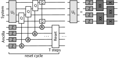
Figure 2: Scheme of our dissipative transverse field Ising realization, similar to Refs. [1, 8] and realistic to implement with a digital quantum computer. In this setup, the system’s qubits are coupled to ancillary ones. After every $T$ system-ancilla-coupling propagations, ancilla qubits are reset to the spin-down state.

We again use periodic boundary conditions for the system’s gates under which the system’s propagation operator factorizes over momenta

$$U_{S}=\prod_{q\geq 0}e^{-i\Phi_{q}^{\dagger}X_{q}\Phi_{q}}e^{-i\Phi^{\dagger}_{q}Z_{q}\Phi_{q}},$$ (22)

with $\Phi_{q}=\{c_{q},c_{-q}^{\dagger}\}^{T}$ representing the bispinor of fermionic operators in momentum space, Eq. (8). $X_{q}$ and $Z_{q}$ are 2x2 matrices, derived by representing the first and the second term in $U_{S}$, Eq. (17), with fermionic operators in the momentum space, using relations (7, 8). Explicit expressions for $X_{q},Z_{q}$ are given in App. A, where we also derive that Floquet quasi-energy dispersion $\tilde{\epsilon}_{q}$ takes the form

$$\cos(\tilde{\epsilon}_{q})=\cos(\pi J)\cos(\pi h)-\sin(\pi J)\sin(\pi h)\cos(q).$$ (23)

Coefficients $\tilde{u}_{q},\tilde{v}_{q}$, connecting fermionic operators to the Bogoliubov ones via relation $c_{q}=\tilde{u}_{q}d_{q}-\tilde{v}^{*}_{q}d_{-q}^{\dagger}$, are for the trotterized transverse field Ising model of the form

$$\tilde{u}_{q} =\frac{(\xi_{q}+\tilde{a}_{q})}{\sqrt{2\xi_{q}(\xi_{q}+\tilde{a}_{q})}},\ \tilde{v}_{q}=\frac{\tilde{b}_{q}}{\sqrt{2\xi_{q}(\xi_{q}+\tilde{a}_{q})}},$$ (24)

$$\tilde{a}_{q} =\sin(\pi J)\cos(\pi h)\cos(q)+\cos(\pi J)\sin(\pi h),$$

$$\tilde{b}_{q} =-e^{-i\pi h}\sin(\pi J)\sin(q),$$

$$\xi_{q} =\sqrt{\tilde{a}_{q}^{2}+|\tilde{b}_{q}}|^{2},$$

which is very similar to the original (9). See App. A for the derivation. Finally,

$$H_{\text{FTFI}}=\sum_{q}\tilde{\epsilon}_{q}\left(n_{q}-\frac{1}{2}\right),\ n_{q}=d_{q}^{\dagger}d_{q}.$$ (25)

Following Ref. [50], we derive the system’s density matrix evolution for one reset cycle, from cycle number $N_{c}$ to $N_{c}+1$. As in the previous section, we approximate the system’s density matrix with a generalized Gibbs ensemble, $\rho_{\bm{\mu}}(N_{c})=(1/Z)e^{-\sum_{q}\mu_{q}(N_{c})n_{q}}$, which should well approximate the exact density matrix time evolution for a weak system-ancilla coupling $\lambda_{\tau}\ll 1$, see also [16],

$$\rho_{\bm{\mu}}(N_{c}+1)-\rho_{\bm{\mu}}(N_{c})$$ (26)

$$\hskip 8.5359pt\approx\sum_{j,\omega,\omega^{\prime}}-i\,\rm{Im}(\mathcal{A}_{\omega,\omega^{\prime}})[Q_{j,\omega^{\prime}}^{\dagger}Q_{j,\omega},\rho_{\bm{\mu}}(N_{c})]$$

$$\hskip 11.38092pt+\mathfrak{a}_{\omega,\omega^{\prime}}\Big{(}Q_{j,\omega}\rho_{\bm{\mu}}(N_{c})Q_{j,\omega^{\prime}}^{\dagger}-\frac{1}{2}\{Q_{j,\omega^{\prime}}^{\dagger}Q_{j,\omega},\rho_{\bm{\mu}}(N_{c})\}\Big{)}.$$

Above we introduced

$$\mathfrak{a}_{\omega,\omega^{\prime}} =\sum_{\tau=1}^{T}\lambda_{\tau}e^{i\tau(\omega^{\prime}-\pi h_{A})}\sum_{\tau^{\prime}=1}^{T}\lambda_{\tau^{\prime}}e^{-i\tau^{\prime}(\omega-\pi h_{A})},$$ (27)

$$\mathcal{A}_{\omega,\omega^{\prime}} =\sum_{\tau=1}^{T}\sum_{\tau^{\prime}=1}^{\tau}\lambda_{\tau}\lambda_{\tau^{\prime}}e^{i(\omega^{\prime}\tau-\omega\tau^{\prime}+\pi h_{A}(-\tau+\tau^{\prime}))},$$

and $Q_{j,\omega}$, which represents $Q_{j}$ operator (20) projected between many-body eigenstates of $H_{\text{FTFI}}$ that differ in quasi-energy for $\omega$, $Q_{j,\omega}=\sum_{\alpha,\beta,\\ \tilde{E}_{\beta}-\tilde{E}_{\alpha}=\omega}\ket{\alpha}\bra{\alpha}Q_{j}\ket{\beta}\bra{\beta}$. A more detailed derivation of the system’s density matrix time evolution is given in App. B and C.

In the case of weak coupling to ancilla qubits, $\lambda_{\tau}\ll 1$, changes within one reset cycle are small. Therefore, one can still use the Euler propagation method to calculate the time-dependent Lagrange multipliers, parametrizing $\rho_{\bm{\mu}}(N_{c})$, from the rate equations for the $H_{\text{FTFI}}$ mode occupation operators. The latter obtains a compact and meaningful form, similar to the continuous model,

$$\langle n_{q}(N_{c}+1)\rangle-\langle n_{q}(N_{c})\rangle$$ (28)

$$=\frac{2}{N}\sum_{q^{\prime}}g_{q^{\prime},q}\big{(}\langle n_{q^{\prime}}\rangle\langle 1-n_{q}\rangle\mathfrak{a}_{\epsilon_{q^{\prime}}-\epsilon_{q}}-\langle n_{q}\rangle\langle 1-n_{q^{\prime}}\rangle\mathfrak{a}_{\epsilon_{q}-\epsilon_{q^{\prime}}}\big{)}$$

$$\hskip 8.5359pt+\tilde{g}_{q^{\prime},q}\big{(}\langle 1-n_{q^{\prime}}\rangle\langle 1-n_{q}\rangle\mathfrak{a}_{-\epsilon_{q^{\prime}}-\epsilon_{q}}-\langle n_{q}\rangle\langle n_{q^{\prime}}\rangle\mathfrak{a}_{\epsilon_{q^{\prime}}+\epsilon_{q}}\big{)}.$$

For a GGE form of the density matrix, Eq. (26) gets simplified in such a way that only the diagonal contributions $\mathfrak{a}_{\omega}\equiv\mathfrak{a}_{\omega,\omega}$ survive, while the term with $\mathcal{A}_{\omega,\omega^{\prime}}$ drops out completely. One should note that the periodicity $\mathfrak{a}_{\omega}=\mathfrak{a}_{\omega+n2\pi}$ is consistent with quasienergies $\tilde{\epsilon}_{q}$ being defined up to shift in multiples of $2\pi$. Transitions caused by the coupling to the ancillas are thus well behaved in the Floquet sense. While function $\mathfrak{a}_{\omega}$ captures the type of coupling to the ancilla qubits, positive real functions

$$g_{q^{\prime},q}=(1+\cos(q+q^{\prime}))|\tilde{u}_{q^{\prime}}\tilde{u}_{q}-\tilde{v}^{*}_{q^{\prime}}\tilde{v}_{q}|^{2},$$ (29)

$$\tilde{g}_{q^{\prime},q}=(1+\cos(q^{\prime}-q))|\tilde{u}_{q^{\prime}}\tilde{v}_{q}-\tilde{v}^{*}_{q^{\prime}}\tilde{u}_{q}|^{2},$$ (30)

take into account the transverse field Ising parameters.

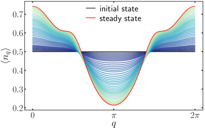
Figure 3: Time evolution of the mode occupation from an initial infinite temperature state. A highly non-thermal steady-state distribution is reached, which could be stabilized by the system-ancilla coupling in a digital quantum computer. Parameters: $J=0.8,h=0.45,h_{A}=0.8,T=6$, $L=500,\lambda_{\tau}=\sqrt{\epsilon}=0.1$.

We consider a time evolution from an initial infinite temperature state with $\mu_{q}=0$, which could be in the digital quantum computer prepared by applying a few layers of (translationally invariant) random two-site gates on some product state [32]. In Fig. 3, we show the (zeroth order) GGE evolution from this state for parameters $J=0.8$, $h=0.45$, $h_{A}=0.8$, $T=6$, $L=500$ and constant $\lambda_{\tau}=\sqrt{\epsilon}=0.1$ for which $\mathfrak{a}_{\omega}=\epsilon\sin^{2}(\frac{T}{2}(\omega-\pi h_{A}))/\sin^{2}(\frac{1}{2}(\omega-\pi h_{A}))$. If the exact density matrix was considered, subleading correction of order $\mathcal{O}(\epsilon^{2})$ would be present. We see that out of a featureless infinite temperature state, some non-thermal features quickly start to appear, and the steady state is reached after approximately $N_{c}\sim 100$ reset cycles for the above parameters. The steady-state itself has a clearly non-thermal occupation of eigenmodes, which depends on the system parameters $J,h$ via function $g_{q^{\prime},q}$, $\tilde{g}_{q^{\prime},q}$ and on the parameters of system-ancilla coupling $h_{A},T$ via function $\mathfrak{a}_{\omega}$. Our main observation is that without a careful shaping of the coupling strength done for the purpose of approximate cooling to the ground state [1, 16], weak constant coupling $\lambda_{\tau}=\sqrt{\epsilon}\ll 1$ of integrable evolution to the ancilla qubits stabilizes a highly non-thermal population of eigenmodes, which depends on the choice of model parameters $J,h,h_{A},T$.

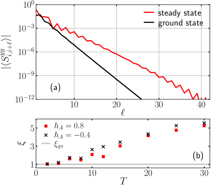
Figure 4: (a) Decay of correlations $|\langle S^{yy}_{i,i+\ell}\rangle|$, Eq. (31), as a function of $\ell$ in the steady-state GGE and the ground state for $h_{A}=0.8,T=6$. As a signature of the stabilized non-thermal GGE, operators that overlap with local conserved quantities of transverse field Ising models show a slower decay of spatial correlations compared to the ground state. (b) Different choices of system-ancilla coupling parameters (field $h_{A}$ and cycle duration $T$) yield different correlation lengths $\xi$. Quite generically, longer cycles lead to slower decay of spatial correlations and thus more non-thermal states. Parameters: $J=0.8,h=0.45,L=500$.

While mode occupation clearly exposes the non-thermal nature of the stabilized state, it cannot be measured directly in a digital quantum computer, which has access only to local observables in the spin language. Local observables, which can expose the non-thermal nature of the stabilized state, are observables that strongly overlap with the local conserved quantities of the transverse field Ising model in the spin language [17, 51],

$$C_{0} =H_{0}$$ (31)

$$C_{2} =\sum_{j}JS^{xx}_{{}_{j,j+2}}-hS^{yy}_{j,j+1}-hS^{xx}_{j,j+1}-J\sigma^{z}_{j}$$

$$C_{2\ell>2} =\sum_{j}JS^{xx}_{{}_{j,j+\ell+1}}-h_{x}S^{yy}_{{}_{j,j+\ell}}-h_{x}S^{xx}_{{}_{j,j+\ell}}+JS^{yy}_{{}_{j,j+\ell-1}}$$

$$C_{2\ell-1} =J\sum_{j}S^{yx}_{{}_{j,j+\ell}}-S^{xy}_{{}_{j,j+\ell}}.$$

where $S^{\alpha\beta}_{i,j}=\sigma^{\alpha}_{i}\sigma^{z}_{i+1}\dots\sigma^{z}_{j-1}\sigma^{\beta}_{j}$. Observables $S^{xx}_{i,j}$ and $S^{yy}_{i,j}$ are experimentally accesible and have been measured also in Ref. [1]. In Fig. 4(a), we plot $|\langle S^{yy}_{i,i+\ell}\rangle|$ in the GGE steady state as a function of $\ell$ and compare it to expectation values in the ground state ($\langle n_{q}\rangle=0$). Because we choose a non-critical set of system parameters, $J=0.8,h=0.45$, ground state and steady state correlations are decaying exponentially. The smoking gun for the GGE stabilization is a slow decay of spatial correlations in the steady state, $|\langle S_{i,i+\ell}^{yy}\rangle|\sim e^{-\ell/\xi}$, which is even slower than the ground state ones, $\xi>\xi_{gs}$. For the chosen Ising parameters $J$ and $h$, $\xi_{gs}\approx 1$, which is not true generically. In Fig. 4(b) we show that with different choices of system-ancilla coupling parameters, one can tune the correlation length $\xi$. Quite generically, a larger number of system-ancilla couplings $T$ induces slower (more non-thermal) decay of spatial correlations. However, this requires a larger number of gates and in total a longer circuit, which comes with a stronger influence of the inherent noise.

A slow decay of correlations in the steady-state for the operators that are overlapping with the conserved quantities of the transverse field Ising model is a direct consequence of reviving effects of integrability. In this case, the integrability is perturbed but also revived due to the dissipative coupling to ancilla qubits. Same would hold in the presence of weak additional unitary integrability breaking or additional native noise: while steady-state would change quantitatively, its non-thermal nature would persist. In that sense these results are rather stable.

V Comparison of approaches for steady-state calculation

Since different approaches to nearly integrable, weakly dissipative system are still rather new [28, 29, 30, 33, 36, 37, 38, 34, 39] and not necessarily fully optimal, we return to the continuous model in this more technical section and compare the performance and complexity of different approaches. A reader not interested in the technical aspects of thermodynamically large calculations for non-interacting models can skip this section and proceed to the Conclusions.

In addition to previously mentioned time evolution from a given initial state, there are other possible approaches to calculating steady-states.
(1) Direct steady-state calculation: If aiming directly for the steady state, one can find the steady state Lagrange parameters $\mu_{q}(t\to\infty)$ from the stationarity condition Eq. (4), $\langle\dot{n}_{q}\rangle=0$ for all momenta. If considering a system of $L$ sites with $L$ mode occupation operators, the complexity of such a root finding procedure is $\mathcal{O}(L^{b+1})$, where $\mathcal{O}(L)$ is the complexity of evaluating the expression $\langle\dot{n}_{q}\rangle$ and $\mathcal{O}(L^{b})$ is the complexity of finding the root for $L$ variables. For example, $b=2$ for Powell method [52].
(2) Iterative steady state calculation: In Ref. [33], we developed an alternative approach, which avoids considering the stationarity conditions for all $\sim L$ conserved quantities (or mode occupation operators) by iteratively constructing the conserved quantities $\tilde{C}_{k}$ which play the leading role in a truncated generalized Gibbs ensemble description of the steady state, $\rho_{\bm{\tilde{\lambda}}}^{(k)}\propto e^{-\sum_{k^{\prime}=0}^{k}\tilde{\lambda}_{k^{\prime}}^{(k)}\tilde{C}_{k^{\prime}}}$. As the zeroth approximation to the steady state a Gibbs ensemble is taken, $\rho_{\bm{\tilde{\lambda}}}^{(0)}\propto e^{-\tilde{\lambda}_{0}^{(0)}H_{0}}$, with the zeroth iterative conserved quantity being the Hamiltonian, $\tilde{C}_{0}=H_{0}$. In the next iterative steps, the $k$th iterative conserved quantity is constructed in some operator basis, which is for non-interacting systems most naturally the basis of mode occupation operators $n_{q}$,

$$\tilde{C}_{k}=\sum_{q}w^{(k)}_{q}n_{q},\ w^{(k)}_{q}\propto\text{Tr}[n_{q}\hat{\mathcal{D}}\rho_{\bm{\tilde{\lambda}}}^{(k-1)}],$$ (32)

see App. E for details. The approximation to the steady state is established by finding Lagrange parameters $\{\tilde{\lambda}_{k^{\prime}}^{(k)}\}$ for $\rho_{\bm{\tilde{\lambda}}}^{(k)}\propto e^{-\sum_{k^{\prime}=0}^{k}\tilde{\lambda}_{k^{\prime}}^{(k)}\tilde{C}_{k^{\prime}}}$ from the set of $k+1$ stationarity conditions $\langle\dot{\tilde{C}}_{k^{\prime}}\rangle=0$, Eq.(4), for $\{\tilde{C}_{k^{\prime}}\}_{k^{\prime}=0}^{k}$. The complexity of the procedure scales as $\mathcal{O}(k^{3}L)$ for the Powell method. If $k\sim\mathcal{O}(1)$ and small, for thermodynamically large systems, the iterative method is clearly advantageous to the previous approach.
(3) Truncated GGE (most local conserved quantities): In principle, another possibility is the truncation in the Fourier modes of $\langle n_{q}\rangle$ or in the number of local conserved quantities $C_{i}$ of the spin model that are considered [28, 30, 31, 53, 26, 17, 54]. $C_{i}$ are for the transverse field Ising model linearly related to the mode occupation operators as $C_{2\ell}=\sum_{q}\cos{(q\ell)}\epsilon_{q}n_{q}$ for even ones ($C_{0}=H_{0}$) and as $C_{2\ell-1}=2J\sum_{q}\sin{(q\ell)}n_{q}$ for odd ones [26]. If one includes only $N_{i}$ most local ones, $2\ell<N_{i}$, then the complexity of finding the truncated steady state GGE scales as $\mathcal{O}(LN_{i}^{2})$.
(4) Time propagation: As done in the previous sections, one can calculate the whole time evolution from some initial $\mu_{q}(0)$, using a discretized version of Eq. (5) and, for example, the Euler method. The complexity of such a calculation is $\mathcal{O}(N_{t}L)$, where $N_{t}$ is the number of steps needed to reach the steady state. If we aim to calculate the steady state, the initial $\mu_{q}(0)$ can be a guess for the steady state. On the other hand, if we aim to describe a realistic time evolution from a state $\ket{\psi_{0}}$, the initial $\mu_{q}(0)$ are given by the initial state through the condition $\langle\psi_{0}|n_{q}|\psi_{0}\rangle=\text{Tr}\left[n_{q}\frac{e^{-\sum_{q^{\prime}}\mu_{q^{\prime}}(0)n_{q^{\prime}}}}{\text{Tr}[e^{-\sum_{q^{\prime}}\mu_{q^{\prime}}(0)n_{q^{\prime}}}]}\right]$. However, this itself is a root-finding procedure which requires $\mathcal{O}(L^{b+1})$ steps.

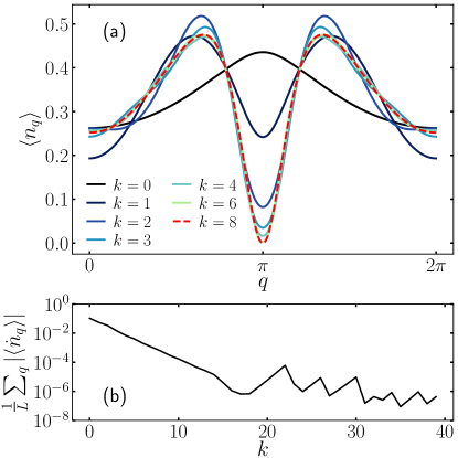
Figure 5: (a) Convergence to the steady state mode occupation at different iterative steps $k$. In the $k=0$ step, the steady state is approximated by a thermal state. In the following iterative steps, additional leading conserved operators are added to a truncated GGE. A decent convergence is obtained in finite number of steps. (b) After the initial improvement of results with increasing number of iterative steps, for chosen parameters, $k>18$ iterative steps fail to improve the results further. However, this happens in the regime where results are converged for all practical purposes. Parameters: $J=1,h=0.6,L=10^{5}$.

The approach (1) is clearly disadvantageous to others and will not be considered. Below we compare approach (4) to the iterative approach (2) from Ref. [33]. We perform the comparison for the model introduced in Sec. III, where the time-dependent calculation (4) has already been performed.

Fig. 5 shows results for the iterative steady-state calculation, Eq. (32). We start with an initial approximation in the form of a Gibbs ensemble, with Hamiltonian being the only conserved quantities. Then, we perform our iterative procedure for constructing a truncated GGE steady-state description. The leading conserved quantities $\tilde{C}_{k}$, Eq. (32), are a linear superposition of the basis mode occupation operators $n_{q}$ with weights selected by the dissipator. Fig. 5 shows momentum distributions obtained after $k$ iterative steps. The initial $k=0$ distribution corresponds to the thermal ensemble at a temperature that best represents the steady state, as obtained from a steady state rate equation for the energy. We observe that convergence to the steady state is obtained in a finite number of $k=8$ steps when we cannot discern this distribution from the ones of the following iterative steps. In Fig. 5(b), we push the number of iterative steps further, even though this is not needed for practical purposes. We observe that improvement is obtained only up to $k=18$ iterative steps. The reason might be that with further steps, we are not adding new direction to the GGE manifold or that we are dealing with extremely small weights in (32) that can be numerically unstable and prone to errors. However, this problematic behavior appears in, for all practical purposes, an irrelevant regime.

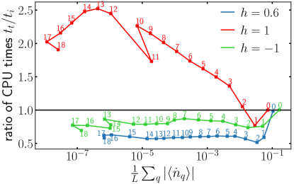
Figure 6: Ratio of computing times $t_{t}/t_{i}$, where $t_{t}$ corresponds to time evolution with $\epsilon\delta t=0.6$ and $t_{i}$ to calculation with the iterative scheme, as a function of $(1/L)\sum_{q}|\langle\dot{n}_{q}\rangle|$, characterizing the accuracy of steady state calculation. Points are labeled by the number of iterative step taken for $t_{i}$ calculation. The two methods are comparable. Which one is more efficient in absolute terms depends on parameters. Parameters: $J=1,L=10^{5}$.

In Fig. 6 we compare the efficiency of the direct time propagation, Eq. (4), and the iterative approach, Eq. (32) by plotting the ratio of CPU times for the former vs the latter. We show that as a function of the average remaining flow of the mode occupations, $(1/L)\sum_{q}|\langle\dot{n}_{q}\rangle|$, characterizing how far from the steady state is the approximate description at a given iterative or finite time step. Fig. 6 reveals that the two methods are comparable, as anticipated from the scaling arguments. Namely, the numerical complexity of time propagation scales as $\mathcal{O}(N_{t}L)$, where $N_{t}$ is the number of propagation steps, while the iterative method scales as $\mathcal{O}(k^{3}L)$, where $k$ is the number of needed iterative steps. For the case studied, direct propagation can be performed at rather large $\epsilon\delta t=0.6$ time steps, meaning that the direct propagation is rather efficient. We could have gained some efficiency for the iterative method by not converging the steady state equations at intermediate iterative steps, however, we did not play with that knob. Which approach is quantitatively advantageous depends on the choice of parameters $J,h$.

In Fig. 7, we plot the steady state expectation values of local conserved quantitites $\langle C_{i}\rangle$, Eq. (31). Since the steady state mode occupation is symmetric, $\langle n_{q}\rangle=\langle n_{-q}\rangle$, only parity-even conserved quantities have finite expectation values. Fig. 7 reveals exponentially decaying contribution with growing support, which indicates that also more standard truncation (3) using the most local conserved quantities is meaningful. If $N_{i}$ conserved quantities are used, the complexity of calculating the steady state scales as $\mathcal{O}(LN_{i}^{2})$. Because we expect that our iterative construction is more efficient, we do not perform a detailed comparison.

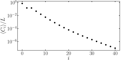
Figure 7: Steady state expectation values of local conserved quantities (31). With increasing support, the importance of even conserved quantities decays exponentially. Expectation values of odd observables are zero due to symmetry. Parameters: $J=1$, $h=0.6,$ $L=10^{5}$.

Our main conclusion from this analysis is that a direct, steady-state calculation (1) of all Lagrange parameters for all the mode occupation operators from the stationarity condition of Eq. (4) is the most costly ($\mathcal{O}(L^{3})$) and should be avoided. Other approaches are comparable; which one is the most efficient depends on the model parameters. Regardless of the method, our first important message is that a weak coupling to non-thermal (Lindblad) baths can stabilize a highly non-thermal steady-state mode occupation. Our second messages is that thermodynamically large calculations can be performed if the GGE ansatz is used as an approximation to the full density matrix description of non-interacting systems weakly coupled to baths.

VI Conclusions

We benchmarked different approaches to non-interacting integrable many-body systems that are weakly coupled to baths and discussed how they could be realized with digital quantum computers, such as superconducting circuits [1] or trapped ions [40].

After mapping the non-interacting model to free fermions, GGEs in terms of mode occupation operators offer a compact interpretation of time evolution and stabilized steady states. Namely, weak integrability breaking perturbations cause scattering between Bogoliubov quasiparticles, and we derived a generalized scattering theory, reminiscent of the Boltzmann equations, which yields the time-dependent eigenmode population, see also [34, 37, 38, 39, 16]. The non-thermal nature of the stabilized steady state can be inferred from the non-Gaussian, structured distribution over eigenmodes, which is related to the transition rates between different quasiparticles caused by the integrability-breaking bath coupling.

We discussed the numerical complexity of different approaches: (1) direct, steady-state calculation, (2) iterative steady-state truncated GGE construction, (3) traditional truncated GGE approximation, and (4) time evolution towards the steady state. We conclude that approach (1) is more expensive than others and should be avoided. We compare (2) and (4) on the example of transverse field Ising model coupled to non-thermal baths and find that they are comparable, in agreement with scaling argument expectations. Which of the two is quantitatively more efficient depends on the model and precise form of coupling to baths. A similar benchmarking for interacting integrable models remains a future challenge.

Notably, we proposed how to realize highly non-thermal GGEs due to proximity to integrability with a digital quantum computer. There, driven-dissipative effects can be implemented by weakly coupling system and ancilla qubits and resetting the latter at the end of every cycle [1]. We derived the effective system’s density matrix time evolution for such a Floquet-reset protocol. By shaping the system-ancilla coupling strength, Ref. [1] recently prepared nearly thermal ensembles with very low temperatures, pushing the system close to the ground state. With our work, we stress that in their case, stabilized states are actually generalized Gibbs ensembles where temperature dominates over other Lagrange parameters due to a particular choice of time-dependent system-ancilla coupling strength. Our example shows that integrable systems that are weakly but generically coupled to ancilla qubits are prone to relax to highly non-thermal GGEs. We comment on how such a highly non-thermal nature could be detected by measuring the decay of correlations that are slower than in the ground state. Additional native noise of the proposed platform should not be a problem and would only slightly alter the time evolution and the steady state while preserving its highly non-thermal nature. A digital quantum computer realization of our proposal would be the first to support a series of theory works [28, 29, 30, 31, 32, 33] revealing a peculiar nature of nearly integrable models that can show a strong non-linear response to weak coupling to non-thermal baths.

Note: During the preparation of this manuscript, a related work appeared on arXiv [16], interpreting the dissipative steady state preparation of Ref. [1] in terms of the scattering theory equivalent to ours.

Appendix A Floquet transverse field Ising model

In this section, we discuss the generalized Bogoliubov rotation for the Floquet transverse field Ising model,

$$U_{S}=e^{-i\frac{\pi J}{2}\sum_{j}\sigma^{x}_{j}\sigma^{x}_{j+1}}e^{-i\frac{\pi h}{2}\sum_{j}\sigma^{z}_{j}}=e^{-iH_{\text{FTFI}}},$$ (33)

relevant for a digital quantum computer realization, Sec. IV. Using the Jordan-Wigner transformation, Eq. (7), the Fourier transform, Eq. (8), and periodic boundary conditions, system’s time evolution factorizes over momenta as

$$U_{S}=\prod_{q\geq 0}e^{-i\Phi_{q}^{\dagger}X_{q}\Phi_{q}}e^{-i\Phi^{\dagger}_{q}Z_{q}\Phi_{q}},$$ (34)

with $\Phi_{q}=\{c_{q},c_{-q}^{\dagger}\}^{T}$ representing the bispinor of fermionic operators in momentum space, Eq. (8) and 2x2 matrices

$$X_{q}=\pi J\begin{bmatrix}\cos(q)&-\sin(q)\\ -\sin(q)&-\cos(q)\end{bmatrix},\quad Z_{q}=\pi h\begin{bmatrix}1&0\\ 0&-1\end{bmatrix}.$$ (35)

Factorization (34) is possible since $X_{q}$ commute amongst each other for positive momenta but not necessarily with their negative momenta counterparts. Dispersion relation $\tilde{\epsilon}_{q}$ and the Bogoliubov transformation are obtained by diagonalizing each $q$-block $e^{-iX_{q}}e^{-iZ_{q}}$ separately,

$$P^{-1}e^{-iX_{q}}e^{-iZ_{q}}P=\text{diag}[e^{-i\tilde{\epsilon}_{q}},e^{-i\tilde{\epsilon}_{-q}}],$$ (36)

yielding

$$\cos(\tilde{\epsilon}_{q})=\cos(\pi J)\cos(\pi h)-\sin(\pi J)\sin(\pi h)\cos(q).$$ (37)

The Bogoliubov transformation, $\Phi_{k}^{\dagger}P=(d_{k}^{\dagger},d_{-k})$, then takes a similar form as in the continuous-time propagation

$$c_{q} =\tilde{u}_{q}d_{q}-\tilde{v}^{*}_{q}d_{-q}^{\dagger},$$ (38)

$$\tilde{u}_{q} =\frac{(\xi_{q}+\tilde{a}_{q})}{\sqrt{2\xi_{q}(\xi_{q}+\tilde{a}_{q})}},\ \tilde{v}_{q}=\frac{\tilde{b}_{q}}{\sqrt{2\xi_{q}(\xi_{q}+\tilde{a}_{q})}},$$

$$\tilde{a}_{q} =\sin(\pi J)\cos(\pi h)\cos(q)+\cos(\pi J)\sin(\pi h),$$

$$\tilde{b}_{q} =-e^{-i\pi h}\sin(\pi J)\sin(q),$$

$$\xi_{q} =\sqrt{\tilde{a}_{q}^{2}+|\tilde{b}_{q}}|^{2}.$$

The system’s unitary time propagator in the diagonal form then equals

$$U_{S}=e^{-i\sum_{q}\tilde{\varepsilon}_{q}(d_{q}^{\dagger}d_{q}-\frac{1}{2})}.$$ (39)

Above we were able to consider the diagonalization of one $q$-block as a matrix, $e^{-iX_{q}}e^{-iZ_{q}}=e^{-iH_{q,\mathrm{FTFI}}}$ Eq. (36), and not as an operator, $e^{-i\Phi_{q}^{\dagger}X_{q}\Phi_{q}}e^{-i\Phi^{\dagger}_{q}Z_{q}\Phi_{q}}=e^{-i\hat{H}_{q,\mathrm{FTFI}}}$, since we can show that $\hat{H}_{q,\mathrm{FTFI}}=\Phi_{q}^{\dagger}H_{q,\mathrm{FTFI}}\Phi_{q}$. This is shown by realizing that for any matrices $\Phi_{q}^{\dagger}A\Phi_{q}$ and $\Phi_{q}^{\dagger}B\Phi_{q}$, where $\Phi_{q}=\{c_{q},c_{-q}^{\dagger}\}^{T}$ is the fermionic bispinor in momentum space, the following commutation relation holds: $[\Phi_{q}^{\dagger}A\Phi_{q},\Phi_{q}^{\dagger}B\Phi_{q}]=\Phi_{q}^{\dagger}[A,B]\Phi_{q}$. From this, it follows that finding the effective Floquet transverse field Ising Hamiltonian for momentum $q$ in the operator form is equivalent to finding it in the matrix form (e.g., via the Baker-Hausdorff-Campbell formula) and applying bispinor operator $\Phi_{q}^{\dagger}$ left and $\Phi_{q}$ right of the Floquet Hamiltonian matrix.

Appendix B Lindblad evolution of system’s density matrix in a digital quantum computer propagation

Here, we derive the discrete time evolution of the system’s density matrix, Eq. (26), for the trotterized gate propagation in a digital quantum computer, where dissipation is due to the coupling and reset of ancillary qubits.

As written in Sec. IV, the system’s time evolution is for one step given by

$$U_{S}=e^{-i\frac{\pi J}{2}\sum_{j}\sigma^{x}_{j}\sigma^{x}_{j+1}}e^{-i\frac{\pi h}{2}\sum_{j}\sigma^{z}_{j}}\equiv e^{-iH_{\text{FTFI}}}.$$ (40)

One step of ancilla qubits time propagation is given by

$$U_{A}=e^{-i\frac{\pi h_{A}}{2}\sum_{j}\tilde{\sigma}^{z}_{j}},$$ (41)

where $\tilde{\sigma}^{\alpha}_{j}$ denotes operators acting on ancilla qubits. This is always followed by a weak hermitian system-ancilla coupling

$$U_{SA,\tau} =\prod_{j}e^{-i\lambda_{\tau}Q_{j}\otimes A_{j}}$$ (42)

$$\approx e^{-i\lambda_{\tau}\sum_{j}Q_{j}\otimes A_{j}-\frac{1}{2}\lambda^{2}_{\tau}\sum_{j,j^{\prime}}[Q_{j},Q_{j^{\prime}}]\otimes A_{j}A_{j^{\prime}}}$$

$$\equiv e^{-iW_{\tau}},$$

where we have introduced $W_{\tau}$ to denote the first and second order of an effective coupling Hamiltonian at time step $\tau\leq T$ before the reset. One cycle contains $T$ system-ancilla-coupling propagations

$$U_{T}=U_{SA,T}U_{A}U_{S}\cdots U_{SA,1}U_{A}U_{S},$$ (43)

followed by a reset of ancilla qubits to spin down state

$$\tilde{P}_{\downarrow}=\hat{\mathbb{1}}\otimes\prod_{j}\frac{1}{2}\left(\tilde{\mathbb{1}}-\tilde{\sigma}_{j}^{z}\right).$$ (44)

Following Ref. [50], we derive the system’s density matrix time evolution in the interaction picture, which is slightly non-standard due to the trotterized nature of the setup. The interaction picture propagator for one cycle (before the reset) equals

$$\mathcal{U}_{T}\equiv U_{0}^{-T}U_{T}=\hat{\mathcal{T}}e^{-i\sum_{\tau=1}^{T}W_{I\tau}},\,U_{0}=U_{A}U_{S},$$ (45)

where $W_{I\tau}=U_{0}^{-\tau}W_{\tau}\,U_{0}^{\tau}$ is the first and second order of the effective coupling Hamiltonian (42) propagated in the interaction picture for $\tau$ steps and $\hat{\mathcal{T}}$ is the time ordering operator. In App. C, we prove Eq. (45).

Due to the projection (44), the whole density matrix operator has a product form at the end of each cycle,

$$\rho_{I}(N_{c})=\rho_{S,I}(N_{c})\otimes\prod_{j}\frac{1}{2}\big{(}\tilde{\mathbb{1}}-\tilde{\sigma}_{j}^{z}\big{)}.$$ (46)

One cycle evolution of the system’s density matrix $\rho_{S,I}$, obtained by tracing out the ancilla qubits, is approximated to second order in coupling strength $\lambda_{\tau}$ by

$$\rho_{S,I}(N_{c}+1)-\rho_{S,I}(N_{c})$$ (47)

$$=\text{Tr}_{A}\Big{(}\mathcal{U}_{T}\rho_{I}(N_{c})\,\mathcal{U}_{T}^{\dagger}\Big{)}-\rho_{S,I}(N_{c})$$

$$\approx-i\text{Tr}_{A}\Big{(}\sum_{\tau=1}^{T}[W_{I\tau},\rho]\Big{)}$$ (48)

$$\hskip 14.22636pt-\text{Tr}_{A}\Big{(}\sum_{\tau=1}^{T}\sum_{\tau^{\prime}=1}^{\tau}[\lambda_{\tau}V_{I\tau},[\lambda_{\tau^{\prime}}V_{I\tau^{\prime}},\rho_{I}(N_{c})]]\Big{)}$$ (49)

$$=\sum_{\tau=1}^{T}\sum_{\tau^{\prime}=1}^{\tau}\sum_{j}\lambda_{\tau}\lambda_{\tau^{\prime}}$$ (50)

$$\hskip 14.22636pt\times\Big{(}\big{(}Q_{j,I\tau}Q_{j,I\tau^{\prime}}\rho_{S,I}(N_{c})-Q_{j,I\tau^{\prime}}\rho_{S,I}(N_{c})Q_{j,I\tau}\big{)}\mathcal{A}_{\tau,\tau^{\prime}}$$

$$\hskip 19.91684pt+\big{(}\rho_{S,I}(N_{c})Q_{j,I\tau^{\prime}}Q_{j,I\tau}-Q_{j,I\tau}\rho_{S,I}(N_{c})Q_{j,I\tau^{\prime}}\big{)}\mathcal{A}^{*}_{\tau,\tau^{\prime}}\Big{)}.$$

The linear term (48) vanishes for our choice $A_{j}=\tilde{\sigma}_{j}^{x}$ since $\text{Tr}_{A}\big{(}U_{0}^{-\tau}A_{j}U_{0}^{\tau}(\tilde{\mathbb{1}}-\tilde{\sigma}_{j}^{z})\big{)}=0$. Generically, it can be set to zero by shifting the $A_{j}$ operators [50]. In a compact notation, the result of resetting and tracing over the ancilla qubits is represented by $\mathcal{A}_{\tau,\tau^{\prime}}$, which for our choice $A_{j}=\tilde{\sigma}_{j}^{x}$ simplifies to

$$\mathcal{A}_{\tau,\tau^{\prime}}\delta_{i,j} =\text{Tr}_{A}\Big{[}\prod_{k}\frac{1}{2}\big{(}\tilde{\mathbb{1}}-\tilde{\sigma}_{k}^{z}\big{)}A_{j,I\tau}A_{i,I\tau^{\prime}}\Big{]}$$

$$=e^{-i\pi h_{A}(\tau-\tau^{\prime})}\delta_{i,j}$$ (51)

Furthermore, we define

$$\mathcal{A}_{\omega,\omega^{\prime}} =\sum_{\tau=1}^{T}\sum_{\tau^{\prime}=1}^{\tau}\lambda_{\tau}\lambda_{\tau^{\prime}}e^{i\omega^{\prime}\tau-i\omega\tau^{\prime}}\mathcal{A}_{\tau,\tau^{\prime}}=\mathfrak{a}_{\omega,\omega^{\prime}}-\mathcal{A}^{*}_{\omega^{\prime},\omega}$$

$$\mathfrak{a}_{\omega,\omega^{\prime}} =\sum_{\tau=1}^{T}\lambda_{\tau}e^{i(\omega^{\prime}-\pi h_{A})\tau}\sum_{\tau^{\prime}=1}^{T}\lambda_{\tau^{\prime}}e^{-i(\omega-\pi h_{A})\tau^{\prime}}$$ (52)

and

$$Q_{j,\omega}=\sum_{\alpha,\beta,\\ \tilde{E}_{\beta}-\tilde{E}_{\alpha}=\omega}\ket{\alpha}\bra{\alpha}Q_{j}\ket{\beta}\bra{\beta},$$ (53)

which represents $Q_{j}$ operator projected between many-body eigenstates of $H_{\text{FTFI}}$ that differ in energy for $\omega$, such that

$$Q_{j,I\tau}=\sum_{\omega}U_{0}^{-\tau}Q_{j,\omega}U_{0}^{\tau},=\sum_{\omega}e^{-i\omega\tau}Q_{j,\omega},$$ (54)

Putting all these together, we derive a compact form

$$\rho_{S,I}(N_{c}+1)-\rho_{S,I}(N_{c})$$ (55)

$$\approx\sum_{j,\omega,\omega^{\prime}}-i\,{\rm Im}(\mathcal{A}_{\omega,\omega^{\prime}})[Q_{j,\omega^{\prime}}^{\dagger}Q_{j,\omega},\rho_{S,I}(N_{c})]$$

$$\hskip 2.84544pt+\mathfrak{a}_{\omega,\omega^{\prime}}\Big{(}Q_{j,\omega}\rho_{S,I}(N_{c})Q_{j,\omega^{\prime}}^{\dagger}-\frac{1}{2}\{Q_{j,\omega^{\prime}}^{\dagger}Q_{j,\omega},\rho_{S,I}(N_{c})\}\Big{)}.$$

To obtain the propagation equation (26) presented in the main text, we approximate the system’s density matrix with a GGE ansatz that, notably, does not evolve under $U_{0}$, making the transformation back to the Schrödinger picture trivial.

Appendix C Floquet interaction picture time propagator

In this section, we show that $\mathcal{U}_{T}$, Eq. (45), is really the interaction picture propagator for one cycle consisting of $T$ system-ancilla-coupling propagations.

The Schrödinger picture propagator (43) can be written as

$$U_{T} =U_{SA,T}U_{A}U_{S}\cdots U_{SA,1}U_{A}U_{S},$$ (56)

$$=U_{SA,T}U_{0}U_{SA,T-1}U_{0}\cdots U_{SA,1}U_{0}$$

$$=\mathbb{1}U_{SA,T}U_{0}\mathbb{1}U_{SA,T-1}U_{0}\cdots\mathbb{1}U_{SA,1}U_{0}$$

$$=U_{0}^{T}\prod_{\tau=1}^{T}U_{I,SA,\tau},$$

where the leftmost identity is $U_{0}^{T}U_{0}^{-T}$, next one $U_{0}^{T-1}U_{0}^{-(T-1)}$ and the rightmost $U_{0}U_{0}^{-1}$. Above we also introduce the interaction picture coupling propagator $U_{I,SA,\tau}=U_{0}^{-\tau}U_{SA,\tau}U_{0}^{\tau}\approx e^{-iW_{I\tau}}$ at step $\tau$. The interaction picture time propagator for one reset cycle of length $T$ is then

$$\mathcal{U}_{T}=U_{0}^{-T}U_{T}=\prod_{\tau=1}^{T}e^{-iW_{I\tau}}=\hat{\mathcal{T}}e^{-i\sum_{\tau=1}^{T}W_{I\tau}}$$ (57)

In the last step, we used the following property of the time ordering operator: $e^{-i\hat{O}(t_{2})}e^{-i\hat{O}(t_{1})}=\hat{\mathcal{T}}e^{-i(\hat{O}(t_{2})+\hat{O}(t_{1}))}$ for any operator $\hat{O}(t)$, if $t_{2}>t_{1}$. Thus, we have shown that Eq. (45) holds.

Appendix D Examples and symmetries in the trotterized setup

In order to illustrate the great variety of different non-thermal steady states stabilized, we show here a few examples of steady state mode occupations that were considered to demonstrate anomalously long spatial correlations in the main text, Fig. 4(b). In Fig. 8, we show the full time evolution of the mode occupation from the initial infinite temperature state, for $J=0.8,h=0.45,h_{A}=-0.4,T=6$. It is interesting to observe that even though these parameters yield a comparable correlation length $\xi$ for the decay of spatial correlations in Fig. 4(b) as $h_{A}=0.8$, the steady state distribution is completely different from the distribution at $h_{A}=0.8$ shown in the main text, Fig. 3.

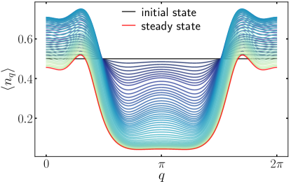
Figure 8: Time evolution of the mode occupation from an initial infinite temperature state. Evolution correspond to the system-ancilla coupling in a digital quantum computer at parameters: $J=0.8,h=0.45,h_{A}=-0.4,T=6$, $L=500,\lambda_{\tau}=\sqrt{\epsilon}=0.1$.

In Fig. 9, we show the steady state distributions of momentum occupations at three different lengths of the reset cycle, $T=2,6,30$, again for parameters $J=0.8,h=0.45,h_{A}=0.8,L=500,\lambda_{\tau}=\sqrt{\epsilon}=0.1$ shown in the main text in Fig. 4(b). Consistently with results from the main text, longer reset-cycles lead to more clearly non-thermal steady states yielding longer spatial correlations in $|\langle S_{i,i+\ell}^{yy}\rangle|$.

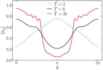
Figure 9: Steady state distributions of the mode occupation for different lengths of the reset cycle $T$. Parameters: $J=0.8,h=0.45,h_{A}=0.8,L=500,\lambda_{\tau}=\sqrt{\epsilon}=0.1$ and $T=2,6,30$.

The equations of motion for the mode occupation,

$$\langle n_{q}(N_{c}+1)\rangle-\langle n_{q}(N_{c})\rangle$$ (58)

$$=\frac{2}{N}\sum_{q^{\prime}}g_{q^{\prime},q}\big{(}\langle n_{q^{\prime}}\rangle\langle 1-n_{q}\rangle\mathfrak{a}_{\epsilon_{q^{\prime}}-\epsilon_{q}}-\langle n_{q}\rangle\langle 1-n_{q^{\prime}}\rangle\mathfrak{a}_{\epsilon_{q}-\epsilon_{q^{\prime}}}\big{)}$$

$$\hskip 8.5359pt+\tilde{g}_{q^{\prime},q}\big{(}\langle 1-n_{q^{\prime}}\rangle\langle 1-n_{q}\rangle\mathfrak{a}_{-\epsilon_{q^{\prime}}-\epsilon_{q}}-\langle n_{q}\rangle\langle n_{q^{\prime}}\rangle\mathfrak{a}_{\epsilon_{q^{\prime}}+\epsilon_{q}}\big{)},$$

have certain symmetries, which imply symmetric relations also for the steady state occupations. Since $\mathfrak{a}_{\omega}(-h_{A})=\mathfrak{a}_{-\omega}(h_{A})$, the steady state occupations at $-h_{A}$ are inverted around the infinite temperature value, $\langle n_{q}\rangle(-h_{A})=1/2-\langle n_{q}\rangle(h_{A})$, with respect to the occupations at $h_{A}$, see Fig. 10. This is a consequence of the exchanged roles of $\mathfrak{a}_{\omega}$ between the first and the second, as well as between the third and the fourth term in Eq. (58). Also, $\langle S_{i,i+\ell}^{yy}\rangle(-h_{A})=-\langle S_{i,i+\ell}^{yy}\rangle(h_{A})$. The second symmetry comes from reflecting the Ising parameter $h\rightarrow 1/2-h$. Taking into account the form of functions $g_{q^{\prime},q},\tilde{g}_{q^{\prime},q}$, Eq. (30), one gets $\langle n_{q}\rangle(1/2-h)=1/2-\langle n_{q+\pi}\rangle(h)$, see Fig. 10. Under this transformation only the correlations between even distances get a minus sign, $\langle S_{i,i+2\ell}^{yy}\rangle(1/2-h)=-\langle S_{i,i+2\ell}^{yy}\rangle(h)$. Same properties hold for the $J\rightarrow 1/2-J$ transformation. In addition to the symmetries discussed above, the equations of motion are invariant under shifting Ising parameters $J,h$ and bath field $h_{A}$ by multiples of $2$.

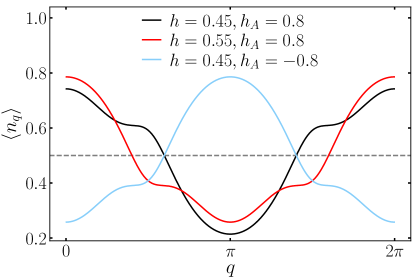
Figure 10: Steady-state mode occupations under different symmetry transformations of the model. Taking $h_{A}\rightarrow-h_{A}$ will invert the steady state population, whereas $h\rightarrow 1/2-h$ will invert the population and shift momentum by $\pi$. Parameters: $J=0.8,T=6,L=500$, $\lambda_{\tau}=\sqrt{\epsilon}=0.1$.

Appendix E Iterative construction of the leading conserved quantities

In Ref. [33], we developed an iterative approach for constructing the conserved quantities $\tilde{C}_{k}$, which play the leading role in a truncated generalized Gibbs ensemble description of the steady state, $\rho_{\bm{\tilde{\lambda}}}^{(k)}\propto e^{-\sum_{k^{\prime}=0}^{k}\tilde{\lambda}_{k^{\prime}}^{(k)}\tilde{C}_{k^{\prime}}}$. As the zeroth approximation to the steady state a Gibbs ensemble is taken, $\rho_{\bm{\tilde{\lambda}}}^{(0)}\propto e^{-\tilde{\lambda}_{0}^{(0)}H_{0}}$, with the zeroth iterative conserved quantity being the Hamiltonian, $\tilde{C}_{0}=H_{0}$. In next iterative steps, the $k$th iterative conserved quantity is constructed in the basis $Q_{m}$, $[H_{0},Q_{m}]=0$ as

$$\tilde{C}_{k} =\mathcal{N}_{k}^{-1}\sum_{m}w^{(k)}_{m}Q_{m},$$

$$w^{(k)}_{m} =-\sum_{n}\left(\chi_{(k-1)}^{-1}\right)_{mn}\text{Tr}[Q_{n}\hat{\mathcal{D}}\rho_{\bm{\tilde{\lambda}}}^{(k-1)}].$$ (59)

For the non-interacting $H_{0}$, a natural choice of basis is the basis of mode occupation operators, $Q_{m}=n_{m}$. In this case, the susceptibility matrix $(\chi_{(k)})_{m,n}=\langle Q_{m}Q_{n}\rangle_{\rho_{\bm{\tilde{\lambda}}}^{(k)}}-\langle Q_{m}\rangle_{\rho_{\bm{\tilde{\lambda}}}^{(k)}}\langle Q_{n}\rangle_{\rho_{\bm{\tilde{\lambda}}}^{(k)}}$ is diagonal $(\chi_{(k)})_{m,n}=e^{-\mu_{m}^{(k)}}/(1+e^{-\mu_{m}^{(k)}})^{2}\delta_{m,n}$ which further reduces the complexity of performing the iterative procedure. Here, $\mu_{m}^{(k)}$ is an effective Lagrange parameter associated to the mode occupation operator $n_{m}$ at $k$th iterative step, $\mu_{m}^{(k)}=\tilde{\lambda}_{0}^{(k)}\varepsilon_{m}+\sum_{k^{\prime}=1}^{k}\mathcal{N}_{k^{\prime}}^{-1}\tilde{\lambda}_{k^{\prime}}^{(k)}w^{(k^{\prime})}_{m}$, and $\varepsilon_{m}$ is the dispersion. The approximation to the steady state is established by finding $\{\tilde{\lambda}_{k^{\prime}}^{(k)}\}$ for $\rho_{\bm{\tilde{\lambda}}}^{(k)}\propto e^{-\sum_{k^{\prime}=0}^{k}\tilde{\lambda}_{k^{\prime}}^{(k)}\tilde{C}_{k^{\prime}}}$ from the set of $k+1$ conditions $\langle\dot{\tilde{C}}_{k^{\prime}}\rangle=0$, Eq.(4), for $\{\tilde{C}_{k^{\prime}}\}_{k^{\prime}=0}^{k}$. We set normalization $\mathcal{N}_{k}$ to be $1$, thereby absorbing it into the corresponding Lagrange parameters.