Quantum Geometry and Entanglement in Two-dimensional Insulators:
A View from the Corner Charge Fluctuation

Abstract

Measuring bipartite fluctuations of a conserved charge, such as the particle number, within a finite region is a powerful approach to characterizing quantum systems. When the measured region has sharp corners, the bipartite fluctuation receives an additional contribution known to exhibit universal angle-dependence in 2D isotropic and uniform systems. Here we establish that the corner charge fluctuation reveals universal information even for generic lattice systems of non-interacting electrons. We first prove that universal angle-dependence can be recovered in the small-angle limit for proper partitions of the lattice, from which the integrated Fubini-Study quantum metric can be extracted. A model of a compact obstructed atomic insulator is introduced to illustrate this effect analytically. Numerical verification is presented for various Chern insulator models, demonstrating the experimental relevance of the corner charge fluctuation in a finite-size quantum simulator as a probe of quantum geometry. Last but not least, we highlight a remarkable connection between quantum geometry and quantum information through the lens of corner entanglement entropies.

Introduction. Quantum geometry has emerged as a new theme in the study of quantum matter by characterizing the groundstate wavefunction through the quantum geometric tensor (QGT) Törmä (2023); Resta (2011); Provost and Vallee (1980). The imaginary part of the QGT is the well-known nonabelian Berry curvature whose trace gives the Chern number after integration Thouless et al. (1982), while the real part gives the quantum metric that determines localization properties of wavefunctions Kivelson (1982); Marzari and Vanderbilt (1997); Resta and Sorella (1999). The integrated Fubini-Study quantum metric of a band insulator is defined as

$$\mathcal{G}_{ij}\equiv\int_{BZ}[d{\bf k}]\;g_{ij}({\bf k}),$$ (1)

where the measure is $[d{\bf k}]\equiv d^{D}{\bf k}/(2\pi)^{D}$, with $D=2$ being the focus of this work, and the integral is over the first Brillouin zone. The integrand $g_{ij}({\bf k})=\frac{1}{2}\tr[\partial_{i}P({\bf k})\partial_{j}P({\bf k})]$ is the ${\bf k}$-space quantum metric tensor, with $\tr$ represents tracing over the orbital basis and $P({\bf k})$ the projector onto the occupied bands. The trace of the integrated metric $\mathcal{G}\equiv\sum_{i=1}^{D}\mathcal{G}_{ii}$ bears a precise meaning as the gauge-invariant part of the Wannier spread functional Marzari and Vanderbilt (1997), and is lower bounded by many kinds of band topology Roy (2014); Peotta and Törmä (2015); Xie et al. (2020); Yu et al. (2022); Herzog-Arbeitman et al. (2022a).

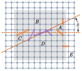
Figure 1: Partition of a square lattice defining the charge fluctuations and entanglement entropies. All quantities are constructed upon the shaded bulk region to eliminate edge effects. The corner charge fluctuation defined in Eq. (6) is a direct observable for quantum geometry of the band insulator on this lattice. Purple (orange) bonds represent the corner (boundary) contribution.

While ideas from quantum geometry have proved useful in understanding fractional Chern insulators Parameswaran et al. (2012); Dobardžić et al. (2013); Roy (2014); Jackson et al. (2015); Claassen et al. (2015); Wang et al. (2021a); Ledwith et al. (2023); Liu and Bergholtz (2024), flat-band superconductivity Peotta and Törmä (2015); Törmä et al. (2022); Huhtinen et al. (2022); Herzog-Arbeitman et al. (2022b); Chen and Law (2024) and electron-phonon coupling Yu et al. (2024), only a few kinds of direct observables have been known for the quantum metric in condensed matter Souza et al. (2000); Neupert et al. (2013); Gianfrate et al. (2020); Ahn et al. (2022); de Sousa et al. (2023); Onishi and Fu (2024a); Kruchkov and Ryu (2023a, b); Onishi and Fu (2024b). Furthermore, while one intuitively expects connections between quantum geometry and quantum entanglement due to their shared relation to wavefunction localization Ryu and Hatsugai (2006); Paul (2024), a precise and quantitative connection is yet to be established. Here we aim to address these issues by studying the bipartite fluctuation of particle number (henceforth referred to as “charge”). Charge fluctuation has shown great promise in revealing universal aspects of quantum critical systems Rachel et al. (2012); Song et al. (2012); Wu et al. (2021); Wang et al. (2021b); Estienne et al. (2022), as well as topology of metals Tam et al. (2022); Tam and Kane (2024). We now add the quantum geometry of two-dimensional (2D) band insulators to that list.

General considerations. For a region $A$ whose shape contains a corner of angle $\theta$, as depicted in Fig. 1, its bipartite charge fluctuation behaves in the continuum as

$$\langle Q^{2}_{A}\rangle_{c}\equiv\langle Q^{2}_{A}\rangle-\langle Q_{A}\rangle^{2}=\alpha\absolutevalue{\partial A}-b(\theta)+...,$$ (2)

where $Q_{A}$ is the particle number operator for $A$. The dominant term is the boundary-law contribution scaling with the length of the boundary $\partial A$, the subdominant constant term $b(\theta)$ is the corner contribution arising from the singular shape of $A$, and the ellipses represent terms vanishing in the thermodynamic limit. Since the boundary-law coefficient $\alpha$ is dimensionful, it is non-universal and not expected to capture the dimensionless integrated quantum metric in 2D. A natural place to hunt for the quantum geometric effect is thus the corner term. In the isotropic and uniform limit, it has been shown that the corner term exhibits a universal angle-dependence Wu et al. (2021); Wang et al. (2021b); Estienne et al. (2022):

$$b(\theta)=\gamma\beta(\theta),\quad\beta(\theta)=\frac{1+(\pi-\theta)\cot\theta}{4\pi^{2}}$$ (3)

where the corner coefficient $\gamma=\pi\nabla^{2}_{\bf q}S_{\bf q}|_{{\bf q}=0}$ is related to the quadratic coefficient of the static structure factor at wavevector ${\bf q}$ Estienne et al. (2022).

Separately, $\pi\nabla^{2}_{\bf q}S_{\bf q}|_{{\bf q}=0}$ has been recently advertised as the “quantum weight” of an insulator Onishi and Fu (2024b), in relation to the negative-first moment of optical conductivity Souza et al. (2000); Resta (2011) and universal bounds determined by material parameters such as the energy gap Kivelson (1982); Onishi and Fu (2024a). For band insulators, the quantum weight is known to be proportional to the integrated quantum metric . This can be appreciated by expressing the density operator as

$$\rho_{\bf q}=\sum_{{\bf k},\sigma mn}U^{\dagger}_{m,\sigma}({\bf k})U_{\sigma,n}({\bf k}+{\bf q})c^{\dagger}_{{\bf k},m}c_{{\bf k}+{\bf q},n},$$ (4)

where $c_{\mathbf{k},n}$ is the electron annihilation operator in the $n$-th band with eigenvector $U_{\sigma,n}(\mathbf{k})$, where $\sigma$ indexes the orbital. From Wick’s contraction, the connected correlator is $\braket{c^{\dagger}_{{\bf k},m}c_{{\bf k}+{\bf q},n}c^{\dagger}_{{\bf k}^{\prime},m^{\prime}}c_{{\bf k}^{\prime}-{\bf q},n^{\prime}}}_{c}=\delta_{{\bf k},{\bf k}^{\prime}-{\bf q}}\bar{\delta}_{m,n^{\prime}}(1-\bar{\delta}_{n,m^{\prime}})$, where $\bar{\delta}_{m,n^{\prime}}$ is the Kronecker delta when $m,n^{\prime}$ are occupied and zero otherwise. The structure factor is thus

$$\begin{split}S_{\bf q}&=\frac{1}{\mathcal{A}}\braket{\rho_{\bf q}\rho_{-{\bf q}}}_{c}=\int[d{\bf k}]\tr[P({\bf k})(1-P({\bf k}+{\bf q}))]\\ &=q^{i}q^{j}\int[d{\bf k}]\frac{1}{2}\tr[\partial_{i}P({\bf k})\partial_{j}P({\bf k})]+O(q^{3}),\end{split}$$ (5)

where $\mathcal{A}$ is the area of the system and $P_{\sigma,\sigma^{\prime}}({\bf k})=\sum_{n\in\text{occ.}}U_{\sigma,n}({\bf k})U^{\dagger}_{n,\sigma^{\prime}}({\bf k})$ is the projector onto the occupied bands. Hence $\pi\nabla^{2}_{\bf q}S_{\bf q}|_{{\bf q}=0}=2\pi\mathcal{G}$. Combined with Eq. (3), it is tempting to suggest a general equality between $2\pi\mathcal{G}$ and the corner coefficient $\gamma$. For Landau levels (LLs), this relation is hinted in Ref. Estienne et al. (2022) by noticing that $\gamma=2n+1$ for the $n$-th LL, which is recognized as $2\pi\mathcal{G}$ from the quantum geometric perspective Peotta and Törmä (2015); Ozawa and Mera (2021). Near a topological gap closing transition where the low-energy physics is captured by a Dirac fermion, it is known that the corner coefficient diverges logarithmically in the system size Herviou et al. (2019); Estienne et al. (2022); Wu (2024), which is again consistent with the quantum metric diverging logarithmically in the Dirac mass Thonhauser and Vanderbilt (2006); Onishi and Fu (2024a).

As we will show, the naive presumption of $\gamma=2\pi\mathcal{G}$ is incorrect in general. Nevertheless, we succeed in extending beyond the uniform, isotropic limit to establish a universal relation between the corner charge fluctuation and quantum geometry of a generic band insulator. While the angle-dependence in Eq. (3) no longer holds for all $\theta$, it can be recovered for $\theta\ll 1$ given a proper choice of partition. Importantly, the corner coefficient $\gamma$ is then determined by the integrated quantum metric.

Corner charge fluctuation. Since the partition boundary is intrinsically rough at the lattice scale, the corner term $b(\theta)$ defined via Eq. (2) is ambiguous on a lattice. Instead, we define the corner contribution by the following combination of bipartite charge fluctuations based on Fig. 1:

$$\begin{split}\mathcal{C}^{(Q)}(\theta)&\equiv\frac{1}{2}\Big{[}-\langle Q^{2}_{A}\rangle_{c}-\langle Q^{2}_{B}\rangle_{c}-\langle Q^{2}_{C}\rangle_{c}-\langle Q^{2}_{D}\rangle_{c}\\ &+\langle Q^{2}_{AB}\rangle_{c}+\langle Q^{2}_{CD}\rangle_{c}+\langle Q^{2}_{BC}\rangle_{c}+\langle Q^{2}_{AD}\rangle_{c}\\ &-\langle Q^{2}_{ABCD}\rangle_{c}\Big{]}.\end{split}$$ (6)

Any boundary contribution arising from the correlation of two sites in neighboring regions (i.e., the orange pairs in Fig. 1) is canceled exactly in the above combination, which leaves us with the correlated pairs that connect regions sharing only the “corner” (i.e., the purple pairs). We have judiciously chosen four bulk regions far away from the physical edge to suppress contribution from edge modes that may exist in a topological phase. Substituting the presumed analytical form in the continuum, we define the lattice corner coefficient

$$\gamma^{(Q)}(\theta)=\frac{\mathcal{C}^{(Q)}(\theta)}{\beta(\theta)+\beta(\pi-\theta)},$$ (7)

with $\beta(\theta)$ defined in Eq. (3). Note that the corner charge fluctuation is generally affected by the orientation of cuts. For the partition in Fig. 1 with one cut lying along the $x$-direction, the corresponding quantities are denoted as $\mathcal{C}^{(Q)}_{x}$ and $\gamma^{(Q)}_{x}$, respectively.

Unveiling quantum geometry. Next we prove the key result of this work:

$$4\pi\widetilde{\mathcal{G}}_{ii}=\lim_{\theta\rightarrow 0}\gamma^{(Q)}_{j}(\theta)\quad\;\;(\text{for}\;\;i\perp j)$$ (8)

where $\widetilde{\mathcal{G}}_{ii}$ is the integrated quantum metric evaluated with an origin orbital embedding (i.e., with all orbitals within a unit cell overlapping on a lattice site), whose physical significance will be explained below. We begin from the two-point correlator $\braket{c^{\dagger}_{{\bf R},\sigma}c_{{\bf R}^{\prime},\sigma^{\prime}}}=\mathcal{A}_{\text{cell}}\int[d{\bf k}]e^{-i{\bf k}\cdot({\bf R}_{\sigma}-{\bf R}^{\prime}_{\sigma^{\prime}})}P_{\sigma^{\prime},\sigma}({\bf k})$, with $\mathcal{A}_{\text{cell}}$ the area of a unit cell, and

$$\braket{Q^{2}_{A}}_{c}=\sum_{\sigma,\sigma^{\prime}}\sum_{\begin{subarray}{c}{\bf R}_{\sigma}\in A\\ {\bf R}^{\prime}_{\sigma^{\prime}}\in\bar{A}\end{subarray}}\mathcal{F}_{\sigma,\sigma^{\prime}}({\bf R}_{\sigma}-{\bf R}^{\prime}_{\sigma^{\prime}})$$ (9)

with

$$\begin{split}&\mathcal{F}_{\sigma,\sigma^{\prime}}({\bf R}_{\sigma}-{\bf R}^{\prime}_{\sigma^{\prime}})=\mathcal{A}_{\text{cell}}^{2}\;\times\\ &\int_{BZ}[d{\bf k}][d{\bf k}^{\prime}]e^{-i({\bf k}-{\bf k}^{\prime})\cdot({\bf R}_{\sigma}-{\bf R}^{\prime}_{\sigma^{\prime}})}P_{\sigma^{\prime},\sigma}({\bf k})P_{\sigma,\sigma^{\prime}}({\bf k}^{\prime}).\end{split}$$ (10)

Here ${\bf R}_{\sigma}$ is the position of the $\sigma$-orbital in the unit cell at ${\bf R}$, and $\bar{A}=BCDE$ is complementary to $A$ and we have used $\braket{Q^{2}_{A}}_{c}=-\braket{Q_{A}Q_{\bar{A}}}_{c}$ by the conservation of total charge. Equation (9) provides a precise interpretation of the boundary-law scaling of the bipartite fluctuation: $\braket{Q^{2}_{A}}_{c}$ is contributed by the correlation of pairs of orbitals, ${\bf R}_{\sigma}\in A$ and ${\bf R}^{\prime}_{\sigma^{\prime}}\in\bar{A}$, and due to the nature of short-range correlation in insulators, the dominant contribution comes from having ${\bf R}_{\sigma}$ and ${\bf R}^{\prime}_{\sigma^{\prime}}$ both in proximity to the boundary $\partial A$. Substituting Eq. (9) into Eq. (6) also makes clear why $\mathcal{C}^{(Q)}(\theta)$ should be attributed to the corner charge fluctuation: the contribution from a pair $\{{\bf R}_{\sigma},{\bf R}^{\prime}_{\sigma^{\prime}}\}$ residing in immediate neighboring regions is absent in Eq. (6). For instance, a term associated with $\{{\bf R}_{\sigma}\in A,{\bf R}^{\prime}_{\sigma^{\prime}}\in B\}$ contributes equally to $\braket{Q^{2}_{A}}_{c}$,$\braket{Q^{2}_{B}}_{c}$, $\braket{Q^{2}_{BC}}_{c}$ and $\braket{Q^{2}_{AD}}_{c}$, so the prescribed combination eliminates such a contribution. Altogether,

$$\mathcal{C}^{(Q)}(\theta)=\sum_{\sigma,\sigma^{\prime}}\Big{(}\sum_{\begin{subarray}{c}{\bf R}_{\sigma}\in B\\ {\bf R}^{\prime}_{\sigma^{\prime}}\in D\end{subarray}}+\sum_{\begin{subarray}{c}{\bf R}_{\sigma}\in A\\ {\bf R}^{\prime}_{\sigma^{\prime}}\in C\end{subarray}}\Big{)}\mathcal{F}_{\sigma,\sigma^{\prime}}({\bf R}_{\sigma}-{\bf R}^{\prime}_{\sigma^{\prime}}).$$ (11)

We now stipulate that the partition scheme does not divide any unit cell, i.e., if ${\bf R}\in A$ then ${\bf R}_{\sigma}$ is assigned to subsystem $A$ for all $\sigma$. From Fig. 1, the number of bonds contributing $\mathcal{F}_{\sigma,\sigma^{\prime}}({\bf R}_{\sigma}-{\bf R}^{\prime}_{\sigma^{\prime}})$ to the first sum is

$$\frac{1}{\mathcal{A}_{\text{cell}}}\big{[}({\bf R}-{\bf R}^{\prime})_{y}\cot{\theta}-({\bf R}-{\bf R}^{\prime})_{x}\big{]}({\bf R}-{\bf R}^{\prime})_{y},$$ (12)

where ${\bf R}_{x(y)}$ is the $x(y)$ coordinate of the unit cell position ${\bf R}$. This counting is exact on the square lattice provided that (i) the angle is chosen to satisfy $\cot{\theta}\in 2\mathbb{N}$ and (ii) all subregions are non-empty, containing at least one site. Taking the small angle limit, only the term proportional to the diverging $\cot{\theta}$ needs to be retained. For the second sum, the partition geometry with $\theta\ll 1$ dictates that ${\bf R}_{\sigma}\in A$ and ${\bf R}^{\prime}_{\sigma^{\prime}}\in C$ are far-separated, hence its contribution is suppressed by the short-range nature of insulators. Consequently, for small $\theta$:

$$\begin{split}\mathcal{C}^{(Q)}_{x}(\theta)&=\frac{\cot{\theta}}{2}\sum_{{\bf R}-{\bf R}^{\prime}}\frac{({\bf R}-{\bf R}^{\prime})_{y}^{2}}{\mathcal{A}_{\text{cell}}}\;\sum_{\sigma,\sigma^{\prime}}\mathcal{F}_{\sigma,\sigma^{\prime}}({\bf R}_{\sigma}-{\bf R}^{\prime}_{\sigma^{\prime}})\\ &=\cot{\theta}\int_{BZ}[d{\bf k}]\frac{1}{2}\tr[(\partial_{y}\widetilde{P}({\bf k}))^{2}],\end{split}$$ (13)

where $\widetilde{P}_{\sigma,\sigma^{\prime}}({\bf k})\equiv e^{i{\bf k}\cdot({\bf r}_{\sigma}-{\bf r}_{\sigma^{\prime}})}P_{\sigma,\sigma^{\prime}}({\bf k})$ is the projector evaluated with an origin orbital embedding where all sublattice positions ${\bf r}_{\sigma}=0$, in accordance with the stipulated partition. As $\theta\rightarrow 0$, $\beta(\theta)+\beta(\pi-\theta)\rightarrow(4\pi\theta)^{-1}$, thus

$$\gamma_{x}^{(Q)}(\theta)=4\pi\int_{BZ}[d{\bf k}]\;\widetilde{g}_{yy}({\bf k}).$$ (14)

The same argument applies to any two-dimensional Bravais lattice, and for partition oriented along any crystal axis, hence we arrive at the main result in Eq. (8) for generic band insulators. In the Supplementary sup , we elaborate on the case of triangular lattice, and in light of the embedding-dependence of quantum geometry Haldane (2014); Lim et al. (2015); Simon and Rudner (2020), we also discuss how $\mathcal{G}_{ii}$ of the physical embedding can be extracted in certain cases.

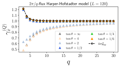
Figure 2: Corner coefficient $\gamma_{x}^{(Q)}$ in the Harper-Hofstadter model, and comparison with the integrated quantum metric $\mathcal{G}_{yy}$.

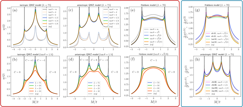
Figure 3: Corner charge fluctuation (left panel) and corner entanglement entropies (right panel) in various Chern insulator models, with the Chern number $C$ indicated in each phase. For charge fluctuation, a universal angle-dependence arises for small $\theta$, where the average corner coefficient $\overline{\gamma}^{(Q)}\equiv\frac{1}{2}(\gamma^{(Q)}_{x}+\gamma^{(Q)}_{y})$ equals to the trace of integrated quantum metric $2\pi\mathcal{G}$. For both the von-Neumann and second Rényi EEs, upon rescaling based on the cumulant expansion, the corresponding average corner coefficients closely follow $2\pi\mathcal{G}$.

Before numerical verifications, let us discuss an analytically solvable model of a compact obstructed atomic insulator on a square lattice Bradlyn et al. (2017); Herzog-Arbeitman et al. (2023), where $\mathcal{C}^{(Q)}(\theta)$ can be evaluated beyond the small-angle-limit (details provided in sup ). This model is constructed with four orbitals on each square lattice site, and the occupied groundstate wavefunction is specified as

$$U({\bf k})=\frac{1}{4}\sum_{m=0}^{3}e^{i\frac{{\bf k}}{2}\cdot(1-C_{4}^{m})(\hat{x}+\hat{y})}\mathcal{D}[C_{4}]^{m}\begin{pmatrix}1\\ 1\\ 1\\ 1\end{pmatrix},$$ (15)

where $C_{4}^{m}$ represents a counter-clockwise rotation by $m\pi/2$, and $\mathcal{D}[C_{4}]=\text{diag}(1,-1,-i,i)$ is the rotation operator in the orbital space. The physical orbital embedding equals to the origin orbital embedding in this model, with $\mathcal{G}_{xx}=\mathcal{G}_{yy}=1/4$. The Wannier orbitals are compactly supported on the four corners of each plaquette, leaving very few terms to include in Eq. (11). As detailed in the Supplementary sup , we find exactly that $\mathcal{C}^{(Q)}(\theta)=\cot{\theta}/4$ for $\cot{\theta}\in 2\mathbb{N}$, and $\mathcal{C}^{(Q)}(\theta)=1/8$ for $\tan{\theta}\in 2\mathbb{N}$. Hence $\gamma^{(Q)}(\theta\ll 1)=\pi$ as promised, while in the opposite limit $\gamma^{(Q)}(\pi/2)=\pi^{2}/4$.

Lattice simulation. We now substantiate our main result, Eq. (8), by simulation of Chern insulator models on lattices of $L\times L$ sites with open boundary conditions. Technical details, including the model Hamiltonians, are provided in sup . To make connection with the Landau-level (LL) physics, we first study the Harper-Hofstadter (HH) model on the square lattice with $2\pi/q$-flux ($q\in\mathbb{Z}$) per plaquette Harper (1955); Hofstadter (1976). The ground state corresponds to occupying the lowest band. As $q\rightarrow\infty$, the lowest band gets flattened and effectively becomes the lowest LL with a uniform quantum geometry and $4\pi\mathcal{G}_{ii}=1$ Peotta and Törmä (2015); Ozawa and Mera (2021). The isotropic and uniform result, Eq. (3), should then hold for all angles, which is confirmed in Fig. 2 where $\gamma_{x}^{(Q)}(\theta)\rightarrow 1$ for all $\theta$. In the lattice regime of small $q$, the continuum result is clearly violated for large angles, but recovered as $\theta\rightarrow 0$ with a corner coefficient matching $4\pi\mathcal{G}_{yy}$. Note that the partition implemented for the HH model (faithfully represented in Fig. 1) may divide the magnetic unit cell, so the argument presented before does not immediately apply. In specific cases with $\tan\theta=1/q$, the unit cell can remain undivided by the partition, and furthermore $\widetilde{\mathcal{G}}_{yy}=\mathcal{G}_{yy}$ as the differences in orbital embeddings are then along $x$, hence the observed match is well explained via Eq. (14). A more general proof of $\gamma^{(Q)}_{x}(\theta\rightarrow 0)=4\pi\mathcal{G}_{yy}$ for the HH model is presented in the Supplementary sup .

To test our theory with a greater variation of quantum geometry, we next study the square-lattice Qi-Wu-Zhang (QWZ) model Qi et al. (2006) and the triangular-lattice Haldane model Haldane (1988). For simplicity, orbitals are located on Bravais lattice sites, hence the physical orbital embedding coincides with the origin orbital embedding. The average corner coefficient $\overline{\gamma}^{(Q)}\equiv\frac{1}{2}(\gamma^{(Q)}_{x}+\gamma^{(Q)}_{y})$ is calculated and compared with the trace of integrated metric $\mathcal{G}=\mathcal{G}_{xx}+\mathcal{G}_{yy}$ in the left panel of Fig. 3. For the QWZ model, we have investigated the isotropic case with hoppings $t_{x}=t_{y}=t$ in Fig. 3(a,b), and the anisotropic case with $t_{x}=2t_{y}=t$ in Fig. 3(c,d). For the Haldane model, we consider nearest-neighbor hopping $t$ and next-nearest-neighbor hopping $t_{2}=0.3t$ with the phase parameter $\phi=\pi/2$ in Fig. 3(e,f). Varying the sublattice mass $M$ we access both trivial and topological phases with varying quantum geometry and $2\pi\mathcal{G}$ lower bounded by the Chern number. While our prediction is made for $\theta\ll 1$, the numerics show an exceptional match between $\overline{\gamma}^{(Q)}$ and $2\pi\mathcal{G}$ already for intermediate $\theta$. Noticeably, a close match can be attained for systems as small as $L=10$. In Supplementary sup , we further demonstrate how $\mathcal{G}$ can be extracted in Haldane’s honeycomb model, where orbitals within a unit cell do not overlap. Given recent realizations of these models in ultracold Fermi gases Jotzu et al. (2014); Liang et al. (2023), our results encourage near-term experimental observation of quantum geometry with the aid of quantum gas microscopy, which offers site-resolved imaging for measuring $\mathcal{C}^{(Q)}$ Cheuk et al. (2015); Haller et al. (2015); Parsons et al. (2015); Edge et al. (2015); Omran et al. (2015); Gross and Bakr (2021).

Corner entanglement entropies. Motivated by the established connection between quantum geometry and corner charge fluctuation, we now explore quantum geometric effects in quantum entanglement. For free fermions concerned in this work, it is well known that the entanglement entropies (EEs) are determined by the full counting statistics composed of charge cumulants Klich and Levitov (2009); Song et al. (2012); Calabrese et al. (2012). We focus on the von-Neumann (vN) and the second Rényi entropies, which satisfy

$$\begin{split}S^{(vN)}_{A}&=\frac{\pi^{2}}{3}\braket{Q^{2}_{A}}_{c}+\frac{\pi^{4}}{45}\braket{Q^{4}_{A}}_{c}+\frac{2\pi^{6}}{945}\braket{Q^{6}_{A}}_{c}+...\\ S^{(2)}_{A}&=\frac{\pi^{2}}{4}\braket{Q^{2}_{A}}_{c}-\frac{\pi^{4}}{192}\braket{Q^{4}_{A}}_{c}+\frac{\pi^{6}}{23040}\braket{Q^{6}_{A}}_{c}+...\end{split}$$ (16)

The EEs are also known to scale generically as Eq. (2), and their corner terms have been studied extensively in conformal field theories Bueno et al. (2015); Hayward Sierens et al. (2017); Bednik et al. (2019); Crépel et al. (2021), and in connection to holographic duality Bueno and Myers (2015); Seminara et al. (2017). Here we discover new connections for non-interacting gapped insulators. The corner entanglement entropies $\mathcal{C}^{(vN,2)}$ are defined similar to Eq. (6), and the corner coefficients $\gamma^{(vN,2)}$ are defined as in Eq. (7). The right panel of Fig. 3 shows the comparison between the average corner EE coefficients $\overline{\gamma}^{(vN,2)}\equiv\frac{1}{2}(\gamma^{(vN,2)}_{x}+\gamma^{(vN,2)}_{y})$ and $2\pi\mathcal{G}$ for small $\theta$, with EEs computed using the standard method of correlation matrix Chung and Peschel (2001); Peschel (2003); Cheong and Henley (2004); sup . The corner EEs are found to closely follow the trend of variation in quantum geometry. Particularly, they peak at gap-closing transitions where the corner EEs are known to diverge logarithmically with the system size Bueno et al. (2015), in consonance with the logarithmic divergence of 2D quantum metric Thonhauser and Vanderbilt (2006); Onishi and Fu (2024a).

Rescaling $\overline{\gamma}^{(vN,2)}$ by the leading coefficient of the cumulant expansion in Eq. (16), a close quantitative match with $2\pi\mathcal{G}$ is observed, though not as accurate as in the case of charge fluctuation. This is understandable because higher-order cumulants have their own corner terms Berthiere et al. (2023). Their quantum geometrical effects are yet to be clarified, which are left for future investigations.

Conclusion. We have demonstrated, both analytically and numerically, that the bipartite charge fluctuation contains a corner term that universally captures the quantum geometry of band insulators on a 2D lattice. We propose a new observable for quantum geometry, which is readily measurable under quantum gas microscopes, and further unveil an intimate relation between quantum geometry and quantum entanglement. Important future directions include extension of our studies to higher dimensions and/or interacting systems. For fractional quantum Hall states, the corner coefficient is known to reflect the fractional filling Estienne et al. (2022); Berthiere et al. (2023), and it would be interesting to explore the corresponding relation to quantum geometry in fractional Chern insulators. This may pave the way to elucidating the role of quantum geometry for the stability of these exotic states, and more broadly speaking, for a finer characterization of interacting topological phases.

Supplementary Materials for “Quantum Geometry and Entanglement in Two-dimensional Insulators: A View from the Corner Charge Fluctuation”
Pok Man Tam, Jonah Herzog-Arbeitman, and Jiabin Yu

The supplemental information consists of four sections. In Sec. I we discuss in detail how to analytically and exactly calculate the corner charge fluctuation in an obstructed atomic insulator with non-trivial quantum geometry. In Sec. II, we explain why our key result in Eq. (8) applies to the triangular lattice, and more generally to any Bravais lattices. In Sec. III, we address subtleties that arise when the physical orbital embedding is different from the origin orbital embedding, with the Harper-Hofstadter model and the Haldane model as our focus. Particularly, we explain how to extract $\mathcal{G}$ of Haldane’s honeycomb model from corner charge fluctuation. In Sec. IV, we first briefly review the correlation matrix method for numerically computing the bipartite fluctuation and entanglement entropies exactly, and collect all the real-space Hamiltonians as well as representative partition configurations used in our numerical studies.

I Compact obstructed atomic insulator

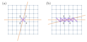
Figure I.1: Corner charge fluctuation in OAI. (a) Partition scheme with $\tan\theta=4$. This is representative for all $\tan\theta\in 2\mathbb{N}$, where only two diagonal bonds contribute to Eq. (I.7). (b) Partition scheme with $\cot\theta=4$. For small angle, the number of bonds contributing to Eq. (I.7) is proportional to $\cot\theta$.

In this section, we study a compact obstructed atomic insulator (OAI) to compute the corner contribution to the charge fluctuation analytically. This analysis complements the other solvable models, the Dirac fermion and Landau levels, where the corner contribution can be analytically calculated by virtue of isotropy as in Ref. Estienne et al. (2022). We build a compact OAI following Ref. Herzog-Arbeitman et al. (2023) using a four-orbital model on the square lattice (with primitive vectors $\hat{x}$ and $\hat{y}$), where $s,d,p_{x},p_{y}$ orbitals are placed at each site with $C_{4}$ representation $D[C_{4}]=\text{diag}(1,-1,-i,i)$. The orthonormal eigenstates ($j=1,2,3,4$) are introduced as follows,

$$U_{j}(\mathbf{k})=\frac{1}{4}\begin{pmatrix}1\\ 1\\ 1\\ 1\end{pmatrix}+\frac{e^{-i\frac{2\pi}{4}j}}{4}\begin{pmatrix}1\\ -1\\ -i\\ i\end{pmatrix}e^{i\mathbf{k}\cdot\hat{x}}+\frac{e^{-i\frac{2\pi}{4}2j}}{4}\begin{pmatrix}1\\ 1\\ -1\\ -1\end{pmatrix}e^{i\mathbf{k}\cdot(\hat{x}+\hat{y})}+\frac{e^{-i\frac{2\pi}{4}3j}}{4}\begin{pmatrix}1\\ -1\\ i\\ -i\end{pmatrix}e^{i\mathbf{k}\cdot\hat{y}}.$$ (I.1)

Each has a Berry connection

$$\mathbf{A}_{j}(\mathbf{k})=U_{j}^{\dagger}(i\boldsymbol{\nabla})U_{j}=-\frac{1}{2}\hat{x}-\frac{1}{2}\hat{y}$$ (I.2)

indicating that the Wannier states built from $U_{j}(\mathbf{k})$ are centered on the plaquette, where there are no atoms. This is a defining feature of an obstructed atomic insulator Bradlyn et al. (2017). Below, we consider a ground state with the $j=0$ band completely occupied and all other bands empty. The parent Hamiltonian of this state can be constructed as $H({\bf k})=-P_{0}({\bf k})=-U_{0}({\bf k})U_{0}^{\dagger}({\bf k})$, and it is easy to check that it describes a tight-binding model with up to second nearest neighbor hoppings. One also easily sees that $g_{xx}({\bf k})=g_{yy}({\bf k})=\frac{1}{2}\tr[(\partial_{i}P_{0}({\bf k}))^{2}]=\frac{1}{4}$. The trace of integrated quantum metric is $\mathcal{G}=\frac{1}{2}$.

To compute the bipartite charge fluctuation, we first construct the Wannier states for the $j$-th band:

$$w^{\dagger}_{{\bf R},j}=\frac{1}{\sqrt{N}}\sum_{{\bf k},\sigma}e^{i{\bf k}\cdot{\bf R}}[U_{j}({\bf k})]_{\sigma}c^{\dagger}_{{\bf k},\sigma}=\sum_{{\bf d},\sigma}[W_{j}({\bf d})]_{\sigma}c^{\dagger}_{{\bf R}+{\bf d},\sigma}\;,\quad\text{with }W_{j}({\bf d})=\frac{1}{N}\sum_{\bf k}e^{-i{\bf k}\cdot{\bf d}}U_{j}({\bf k}).$$ (I.3)

Here $c^{\dagger}_{{\bf k},\sigma}$ and $c^{\dagger}_{{\bf R},\sigma}$ are the fermionic creation operators in the momentum and real spaces, respectively, and $N$ is the number of sites. The inverse transform that we need is

$$c^{\dagger}_{{\bf R},\sigma}=\sum_{{\bf d},j}[V_{j}({\bf d})]_{\sigma}w^{\dagger}_{{\bf R}-{\bf d},j}\;,\quad\text{with }V_{j}({\bf d})=\frac{1}{N}\sum_{\bf k}e^{i{\bf k}\cdot{\bf d}}U^{*}_{j}({\bf k}).$$ (I.4)

It is clear from our construction of the compact OAI that $V_{j}({\bf d})$ and $W_{j}({\bf d})$ are non-zero only for ${\bf d}=0,\hat{x},\hat{y},\hat{x}+\hat{y}$, so each Wannier orbital is compactly supported on four corners of a plaquette. The many-body ground state of our choice corresponds to filling up all Wannier orbitals of the $j=0$ band:

$$\ket{GS}=\prod_{\text{all }{\bf R}}w^{\dagger}_{{\bf R},0}\ket{0},$$ (I.5)

and hence

$$\braket{c^{\dagger}_{{\bf R},\sigma}c_{{\bf R}^{\prime},\sigma^{\prime}}}=\sum_{{\bf d}}[V_{0}({\bf d})]_{\sigma}[V_{0}({\bf d}-{\bf R}+{\bf R}^{\prime})]^{*}_{\sigma^{\prime}}.$$ (I.6)

Now, noting that the bipartite fluctuation can be computed as $\braket{Q^{2}_{A}}_{c}=-\braket{Q_{A}Q_{\bar{A}}}$, so upon substituting into the definition of corner charge fluctuation in Eq. (6), we find

$$\mathcal{C}^{(Q)}(\theta)=\Big{(}\sum_{\begin{subarray}{c}{\bf R}\in B\\ {\bf R}^{\prime}\in D\end{subarray}}+\sum_{\begin{subarray}{c}{\bf R}\in A\\ {\bf R}^{\prime}\in C\end{subarray}}\Big{)}\sum_{\sigma,\sigma^{\prime}}\sum_{{\bf d},{\bf d}^{\prime}}\;[V_{0}({\bf d})]_{\sigma}[V_{0}({\bf d}-{\bf R}+{\bf R}^{\prime})]^{*}_{\sigma^{\prime}}[V_{0}({\bf d}^{\prime})]^{*}_{\sigma}[V_{0}({\bf d}^{\prime}-{\bf R}+{\bf R}^{\prime})]_{\sigma^{\prime}}.$$ (I.7)

This is equivalent to Eq. (11) in the main text, but just written in a convenient form ready for direct evaluation for the OAI model.

Let us now compute $\mathcal{C}^{(Q)}(\theta)$ in two cases: (I) for large angles with $\tan\theta\in 2\mathbb{N}$, and (II) for small angles with $\cot\theta\in 2\mathbb{N}$. For case (I), it is obvious from Fig. I.1(a) that only the two diagonal bonds crossing in the center of the figure contribute. Bond $\{13\}$ corresponds to ${\bf R}-{\bf R}^{\prime}=\hat{x}+\hat{y}$ and ${\bf d}={\bf d}^{\prime}=\hat{x}+\hat{y}$, and contributes $1/16$ to $\mathcal{C}^{(Q)}(\theta)$. By $C_{4}$, one deduces that bond $\{24\}$ also contributes $1/16$, so altogether $\mathcal{C}^{(Q)}=1/8$ in case (I). For case (II), it is obvious from Fig. I.1(b) that three types of bonds contribute: the vertical ones like bond $\{14\}$ and bond $\{23\}$ (altogether $\cot\theta$ of these), the diagonal ones like bond $\{24\}$ (altogether $\cot\theta+1$ of these), and the diagonal ones like bond $\{13\}$ (altogether $\cot\theta-1$ of these). Here, bond $\{14\}$ (and its alike) contributes $1/8$ (as one can choose ${\bf d}={\bf d}^{\prime}=\hat{y}$ and ${\bf d}={\bf d}^{\prime}=\hat{x}+\hat{y}$), and the diagonal bonds again just contribute $1/16$. Altogether we conclude $\mathcal{C}^{(Q)}=\frac{1}{4}\cot\theta$.

II Lattice partition scheme

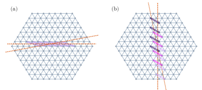
Figure II.1: Partition scheme for the triangular lattice with $\tan\theta=\sqrt{3}/9$. The small angle limit of (a) and (b) gives $\int_{BZ}[d{\bf k}]g_{yy}$ and $\int_{BZ}[d{\bf k}]g_{xx}$, respectively.

In this section, we elaborate on how the argument presented in the main text to establish Eq. (8) can be applied to a generic Bravias lattice. For simplicity we focus on band insulators on a generic Bravais lattice where orbitals of each unit cell overlap on the lattice site. Thus the so-called “origin orbital embedding” is the same as the physical orbital embedding (${\bf r}_{\sigma}=0$, hence ${\bf R}_{\sigma}={\bf R}$). Note also that we do not attempt to provide the most generic lattice partition scheme for extracting the integrated quantum metric $\mathcal{G}_{ii}$. We only provide a sufficient scheme of partition, which is applicable to any Bravais lattice (with the set of angles depending on the microscopic lattice geometry).

II.1 Triangular lattice: a two-orientation scheme

Here we first specify the partition scheme used to extract $2\pi\mathcal{G}$ on a triangular lattice, and later generalize to arbitrary oblique lattices. In particular, we explain why we have chosen the set of angles $\tan\theta=\infty,\sqrt{3},\sqrt{3}/3,\sqrt{3}/9,\sqrt{3}/15$ in our numerics for the Haldane model presented in Fig. 3. In short, just like in the case of a square lattice, they are so chosen such that the partition boundary never intersect any lattice site and that an exact counting similar to Eq. (12) can be attained.

As seen in the main text, we need to consider two kinds of partitions to extract $\mathcal{G}=\mathcal{G}_{xx}+\mathcal{G}_{yy}$: (I) one kind is oriented such that one of the partition boundary is pointing along $\hat{x}$, and (II) another kind is oriented such that one of the partition boundary is pointing along $\hat{y}$. For (I)/(II), we first put the horizontal/vertical boundary in the middle of two central rows/columns, and then lay down the slanted boundary such that it intersects these two central rows/columns at the mid-point of some edges. The “central” rows/columns are picked for convenience, so that after the partition we can specify four bulk subregions that are far away enough from the physical edge of the total system to suppress spurious edge contributions. Cases (I) and (II) are illustrated in Fig. II.1 (a) and (b), respectively, for $\tan\theta=\sqrt{3}/9$. One can appreciate that this is the exact same rationale we used to partition the square lattice in Fig. 1. For (I), it can be seen that the allowed $\theta$ satisfies $\tan\theta=\frac{\sqrt{3}}{2n+1}$ with $n\in\mathbb{Z}$, while for (II) we require $\tan\theta=\frac{\sqrt{3}}{3(2m+1)}$ with $m\in\mathbb{Z}$. The common solutions thus give $\tan\theta=\sqrt{3}/3,\sqrt{3}/9,\sqrt{3}/15$, etc. . Notice also that whenever $\theta$ gives an unambiguous partition, $\pi/2-\theta$ also gives an unambiguous partition, thus we have also considered $\tan\theta=\infty,\sqrt{3}$ in our simulation.

Now let us perform the same analytic argument as in the main text to evaluate Eq. (11) for the triangular lattice given the aforementioned partition scheme. For illustration, focus on Fig. II.1(a) for case (I): given any fixed ${\bf R}-{\bf R}^{\prime}$ on the triangular lattice, the number of such bonds are counted as

$$[\frac{({\bf R}-{\bf R}^{\prime})_{y}}{a}\cot\theta-\frac{({\bf R}-{\bf R}^{\prime})_{x}}{a}]\cdot\frac{({\bf R}-{\bf R}^{\prime})_{y}}{a\sqrt{3}/2},$$ (II.1)

which is the same as Eq. (12) upon recognizing $a^{2}\sqrt{3}/4=\mathcal{A}_{\text{cell}}$. For case (II) in Fig. II.1(b), one again obtain the same expression with $x\leftrightarrow y$, $a\sqrt{3}/2\mapsto a/2$ and $a\mapsto a\sqrt{3}$, which is again Eq. (12). In Fig. IV.1 of the next section, we show some representative partition configurations that we used for producing Fig. 3 of the main text.

The above two-orientation partition scheme works for extracting the trace of integrated metric, $\mathcal{G}=\mathcal{G}_{xx}+\mathcal{G}_{yy}$, as long as the Bravais lattice contains two orthogonal lattice vectors. This, however, is not true for a generic oblique lattice, which requires a three-orientation partition scheme as described next.

II.2 General oblique lattice: a three-orientation scheme

Now consider a generic oblique Bravais lattice with primitive vectors ${\bf a}_{1}$, ${\bf a}_{2}$ and ${\bf a}_{3}=-{\bf a}_{1}-{\bf a}_{2}$. Along each crystal axis ${\bf a}_{i}$, we extract the small-angle corner coefficient based on the partition described above, which gives us

$$\mathcal{C}^{(Q)}_{i}(\theta)=\frac{\cot\theta}{2}\sum_{\Delta{\bf R}}[\Delta{\bf R}\cdot\hat{{\bf b}}_{i}]^{2}\mathcal{F}(\Delta{\bf R}),$$ (II.2)

where $\hat{{\bf b}}_{i}\perp{\bf a}_{i}$ is a unit vector. Denote the angle between $\hat{{\bf b}}_{i}$ and $\hat{{\bf b}}_{j}$ by $\phi_{ij}$. Without loss of generality, assume $\hat{{\bf b}}_{1}=\hat{x}$, then

$$[\Delta{\bf R}\cdot\hat{{\bf b}}_{1}]^{2} =\Delta{\bf R}_{x}^{2}$$ (II.3a)

$$[\Delta{\bf R}\cdot\hat{{\bf b}}_{2}]^{2} =\Delta{\bf R}_{x}^{2}\cos^{2}\phi_{12}+\Delta{\bf R}_{y}^{2}\sin^{2}\phi_{12}+\Delta{\bf R}_{x}\Delta{\bf R}_{y}\sin{2\phi_{12}}$$ (II.3b)

$$[\Delta{\bf R}\cdot\hat{{\bf b}}_{3}]^{2} =\Delta{\bf R}_{x}^{2}\cos^{2}\phi_{13}+\Delta{\bf R}_{y}^{2}\sin^{2}\phi_{13}-\Delta{\bf R}_{x}\Delta{\bf R}_{y}\sin{2\phi_{13}}$$ (II.3c)

It is straighforward to check that

$$\Delta{\bf R}^{2}=\frac{\cos\phi_{23}}{\sin\phi_{12}\sin\phi_{13}}[\Delta{\bf R}\cdot\hat{{\bf b}}_{1}]^{2}+(\text{cyclic permutations of 123}).$$ (II.4)

For the case when the physical orbital embedding is the same as the origin orbital embedding, the trace of the integrated Fubini-Study metric can be extracted as $2\pi\mathcal{G}=\lim_{\theta\rightarrow 0}\overline{\gamma}^{(Q)}(\theta)$ with

$$\overline{\gamma}^{(Q)}=\frac{1}{2}\Big{[}\frac{\cos\phi_{23}}{\sin\phi_{12}\sin\phi_{13}}\gamma^{(Q)}_{1}+(\text{cyclic permutations of 123})\Big{]}.$$ (II.5)

III Orbital Embedding: Physical vs Origin

In this section we address subtleties that arise when the physical orbital embedding is different from the origin orbital embedding. The examples we focus on are the Harper-Hoftstadter model and the Haldane honeycomb model, and their Hamiltonians are provided in Sec. IV.

III.1 Harper-Hofstadter model

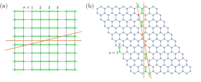
Figure III.1: (a) Partition of the square lattice which supports the Harper-Hofstadter model, with $2\pi/q$-flux per plaquette. For $q=4$, the magnetic unit cell (colored in green) remain undivided by the partition scheme with a corner angle $\tan\theta=1/4$. (b) Partition of the honeycomb lattice which supports the Haldane model. The depicted partition corresponds to a corner with $\tan\theta=\sqrt{3}/9$, and importantly, the partition preserves the unit cell (colored in green) without dividing it.

In the main text, we have used Eq. (14) to explain why for the specific case of $\tan\theta=1/q$ we find $\gamma^{(Q)}_{x}=4\pi\mathcal{G}_{yy}$. We first supplement this argument by referring readers to Fig. III.1(a), where it clearly shows that the chosen magnetic unit cell containing $q$ orbitals are not divided by the partition with corner angle $\theta=\arctan{q^{-1}}$. Notice that the sublattice position difference $({\bf r}_{\sigma}-{\bf r}_{\sigma^{\prime}})\parallel\hat{x}$, hence the physical embedding projector $P_{\sigma,\sigma^{\prime}}({\bf k})$ and the origin orbital embedding projector $\widetilde{P}_{\sigma,\sigma^{\prime}}({\bf k})=e^{i{\bf k}\cdot({\bf r}_{\sigma}-{\bf r}_{\sigma^{\prime}})}P_{\sigma,\sigma^{\prime}}({\bf k})$ differ only by a $k_{y}$-independent unitary transformation. Thus,

$$\widetilde{g}_{yy}=\frac{1}{2}\tr[(\partial_{y}\widetilde{P}({\bf k}))^{2}]=\frac{1}{2}\tr[(\partial_{y}P({\bf k}))^{2}]=g_{yy}.$$ (III.1)

As we have noted in the main text, this argument suffices to explain the match in Fig. 2 for the specific cases with $\tan\theta=1/q$, but it is clear that the exceedingly nice match between $\gamma^{(Q)}_{x}$ and $4\pi\mathcal{G}_{yy}$ holds even more generally when the partition of square lattice can divide the magnetic unit cell. Below we explain this generic phenomenon by adapting the counting argument around Eq. (12) to the generic partition situation.

For readers’ convenience, let us recollect from the main text that the corner charge fluctuation can be expressed as

$$\mathcal{C}^{(Q)}(\theta)=\sum_{\sigma,\sigma^{\prime}}\Big{(}\sum_{\begin{subarray}{c}{\bf R}_{\sigma}\in B\\ {\bf R}^{\prime}_{\sigma^{\prime}}\in D\end{subarray}}+\sum_{\begin{subarray}{c}{\bf R}_{\sigma}\in A\\ {\bf R}^{\prime}_{\sigma^{\prime}}\in C\end{subarray}}\Big{)}\mathcal{F}_{\sigma,\sigma^{\prime}}({\bf R}_{\sigma}-{\bf R}^{\prime}_{\sigma^{\prime}}),$$ (III.2)

with

$$\mathcal{F}_{\sigma,\sigma^{\prime}}({\bf R}_{\sigma}-{\bf R}^{\prime}_{\sigma^{\prime}})=\mathcal{A}_{\text{cell}}^{2}\int_{BZ}[d{\bf k}][d{\bf k}^{\prime}]e^{-i({\bf k}-{\bf k}^{\prime})\cdot({\bf R}_{\sigma}-{\bf R}^{\prime}_{\sigma^{\prime}})}P_{\sigma^{\prime},\sigma}({\bf k})P_{\sigma,\sigma^{\prime}}({\bf k}^{\prime}).$$ (III.3)

To be generally consistent with the implementation of partition we used for the numerics, here we do not invoke the stipulation mentioned just below Eq. (11). Whether ${\bf R}_{\sigma}$ is within a subregion is solely determined by its physical position, making no reference to the unit cell position. Notice that translation symmetry in the Harper-Hofstadter model implies that $\mathcal{F}_{\sigma,\sigma^{\prime}}({\bf R}_{\sigma}-{\bf R}^{\prime}_{\sigma^{\prime}})$ is only explicitly dependent on the positional displacement ${\bf R}_{\sigma}-{\bf R}^{\prime}_{\sigma^{\prime}}$, but not on the sublattice indices, hence for the moment we can write $\mathcal{F}_{\sigma,\sigma^{\prime}}({\bf R}_{\sigma}-{\bf R}^{\prime}_{\sigma^{\prime}})\equiv f({\bf r}-{\bf r}^{\prime})$. Let us also replace $\sum_{\sigma,\sigma^{\prime}}\sum_{{\bf R}_{\sigma}\in B,{\bf R}^{\prime}_{\sigma^{\prime}}\in D}$ by $\sum_{{\bf r}\in B,{\bf r}^{\prime}\in D}$, with ${\bf r}\;({\bf r}^{\prime})$ summed over square lattice sites in region $B$ ($D$). We remark that the above replacement cannot be generalized to an arbitrary multi-orbital model, which is why for an arbitrary model we need to stipulate a special kind of partition, as mentioned below Eq. (11), to arrive at a simple universal result. With our focus on the Harper-Hofstadter model, we realize that given a fixed ${\bf r}-{\bf r}^{\prime}$, the number of terms that contribute to the first sum in Eq. (III.2) is

$$\frac{1}{\mathcal{A}_{\text{plaq.}}}\big{[}({\bf r}-{\bf r}^{\prime})_{y}\cot{\theta}-({\bf r}-{\bf r}^{\prime})_{x}\big{]}({\bf r}-{\bf r}^{\prime})_{y},$$ (III.4)

where $\mathcal{A}_{\text{plaq.}}=\mathcal{A}_{\text{cell}}/q$ is the area of an elementary plaquette on the square lattice. As in the main text, we take the small-angle-limit ($\theta\rightarrow 0$), only retain the $\cot\theta$-term and neglect all of the rest, we obtain

$$\begin{split}\mathcal{C}^{(Q)}_{x}(\theta\rightarrow 0)&=\frac{\cot\theta}{2}\sum_{{\bf r}-{\bf r}^{\prime}}\frac{({\bf r}-{\bf r}^{\prime})_{y}^{2}}{\mathcal{A}_{\text{plaq.}}}f({\bf r}-{\bf r}^{\prime})\\ &=\frac{\cot\theta}{2}\mathcal{A}_{\text{cell}}\sum_{\sigma,\sigma^{\prime}}\sum_{\begin{subarray}{c}{\bf R}_{\sigma}-{\bf R}^{\prime}_{\sigma^{\prime}}\end{subarray}}({\bf R}_{\sigma}-{\bf R}^{\prime}_{\sigma^{\prime}})_{y}^{2}\;\int_{BZ}[d{\bf k}][d{\bf k}^{\prime}]e^{-i({\bf k}-{\bf k}^{\prime})\cdot({\bf R}_{\sigma}-{\bf R}^{\prime}_{\sigma^{\prime}})}P_{\sigma^{\prime},\sigma}({\bf k})P_{\sigma,\sigma^{\prime}}({\bf k}^{\prime})\\ &=\cot{\theta}\int_{BZ}[d{\bf k}]\frac{1}{2}\tr[(\partial_{y}P({\bf k}))^{2}].\end{split}$$ (III.5)

In the second equality, we have replaced $\sum_{{\bf r}-{\bf r}^{\prime}}$ by $\frac{1}{q}\sum_{\sigma,\sigma^{\prime}}\sum_{{\bf R}_{\sigma}-{\bf R}^{\prime}_{\sigma^{\prime}}}$. In the third equality, we have used $({\bf R}_{\sigma}-{\bf R}^{\prime}_{\sigma^{\prime}})_{y}^{2}e^{-i({\bf k}-{\bf k}^{\prime})\cdot({\bf R}_{\sigma}-{\bf R}^{\prime}_{\sigma^{\prime}})}=\partial_{y}\partial_{y^{\prime}}e^{-i({\bf k}-{\bf k}^{\prime})\cdot({\bf R}_{\sigma}-{\bf R}^{\prime}_{\sigma^{\prime}})}$, and subsequently integrated by parts. Note that in the final expression we have the projector $P({\bf k})$ for the physical orbital embedding. We have thus explained the general match between the corner coefficient $\gamma^{(Q)}_{x}$ and $4\pi\mathcal{G}_{yy}$ in Fig. 2.

III.2 Haldane’s honeycomb model

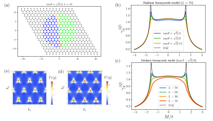
Figure III.2: Extracting $\mathcal{G}$ of the Haldane honeycomb model ($t^{\prime}=0.3t$, $\phi=\pi/2$). (a) shows an example of spatial partition used in our simulation to extract the corner charge fluctuation coefficient $\gamma^{(Q)}_{y}$. (b,c) show the comparison between $2\pi\mathcal{G}$ and $\gamma^{(Q)}_{y}$ for various partition angles and total system sizes. Notice that the trace of integrated metric $\mathcal{G}$ is different for the honeycomb lattice model and the triangular lattice model, by comparing (b,c) here with Fig. 3(e,f). The momentum-space distribution of $\text{Tr}[g]\equiv g_{xx}+g_{yy}$ (for $M=t$) is shown in (d) for the honeycomb lattice model, showing the presence of $C_{3}$ symmetry, and in (e) for the triangular lattice model which lacks $C_{3}$.

In the main text when we studied the Haldane model, we put two overlapping orbitals on each triangular lattice site. From the corner charge fluctuation we are able to extract the trace of integrated quantum metric $\mathcal{G}$, as shown in Fig. 3. For the sake of completeness, and also for convenience of potential quantum gas microscopy endeavor (which may find it challenging to image on-site double occupation), here we demonstrate how $\mathcal{G}$ of the honeycomb model, with spatially displaced sublattices, can be extracted.

Our goal can be achieved by the kind of partition depicted in Fig. III.1(b), which does not divide the unit cell (labeled in green). According to our key result in the main text, Eq. (8), the corner coefficient gives the integrated quantum metric evaluated with the origin orbital embedding. But notice, just like in the above analysis of the Harper-Hofstadter model, here $\widetilde{P}_{\sigma,\sigma^{\prime}}({\bf k})=e^{i{\bf k}\cdot({\bf r}_{\sigma}-{\bf r}_{\sigma^{\prime}})}P_{\sigma,\sigma^{\prime}}({\bf k})$ differ from the physical embedding projector $P({\bf k})$ only by a $k_{x}$-independent unitary transformation, as $({\bf r}_{2}-{\bf r}_{1})\parallel\hat{y}$. Consequently, with small $\theta$, we obtain $\gamma^{(Q)}_{y}=4\pi\widetilde{\mathcal{G}}_{xx}=4\pi\mathcal{G}_{xx}$. To obtain the trace of integrated metric $\mathcal{G}=\mathcal{G}_{xx}+\mathcal{G}_{yy}$, one should not attempt to compute $\gamma^{(Q)}_{x}$ by partitioning the honeycomb lattice along $x$, as that would not give the correct $\mathcal{G}_{yy}$ (one should appreciate from Fig. III.1 that $\widetilde{\mathcal{G}}_{yy}\neq\mathcal{G}_{yy}$). Instead, we can make use of the $C_{3}$ symmetry of the honeycomb Haldane model together with the three-orientation partition scheme based on Eqs. (II.4). With $\phi_{12}=\phi_{23}=\phi_{13}=2\pi/3$, we expect

$$2\pi\mathcal{G}=\frac{4\pi(\mathcal{G}_{xx}+\mathcal{G}_{C_{3}x,C_{3}x}+\mathcal{G}_{C_{3}^{2}x,C_{3}^{2}x})}{3}=4\pi\mathcal{G}_{xx}=\gamma^{(Q)}_{y}.$$ (III.6)

This is confirmed in Fig. III.2.

IV Additional information for numerical studies

IV.1 Correlation matrix method

The central quantity we compute for a subsystem $A$ is its two-point correlation matrix $(C_{A})_{ij}=\langle c^{\dagger}_{i}c_{j}\rangle$, where $i,j\in A$ label all the orbitals inside this subsystem. From this we calculate the bipartite particle-number fluctuation as

$$\braket{Q^{2}_{A}}_{c}=\sum_{i,j\in A}\braket{c^{\dagger}_{i}c_{i}c^{\dagger}_{j}c_{j}}_{c}=\sum_{i\in A}\braket{c^{\dagger}_{i}c_{i}}-\sum_{i,j\in A}\braket{c^{\dagger}_{i}c_{j}}\braket{c^{\dagger}_{j}c_{i}}=\text{Tr}[C_{A}-C_{A}^{2}],$$ (IV.1)

where Tr represents tracing over the orbitals in subsystem $A$. The subscript $c$ means connected correlation. More generally,

$$\langle Q_{A}Q_{B}\rangle_{c}\equiv\langle Q_{A}Q_{B}\rangle-\langle Q_{A}\rangle\langle Q_{B}\rangle=\delta_{AB}\langle Q_{A}\rangle-\sum_{i\in A}\sum_{j\in B}\langle c^{\dagger}_{i}c_{j}\rangle\langle c^{\dagger}_{j}c_{i}\rangle.$$ (IV.2)

The correlation matrix also allows us to compute entanglement entropies (EEs) for free-fermion systems Chung and Peschel (2001); Peschel (2003); Cheong and Henley (2004). In this work we have focused on the von-Neumann EE $S^{(vN)}_{A}=-\text{Tr}[\rho_{A}\log\rho_{A}]$, and the second Rényi EE $S^{(2)}_{A}=-\log\text{Tr}[\rho^{2}_{A}]$. The key idea of the method is to express the reduced density matrix $\rho_{A}$ in an exponential form,

$$\rho_{A}=\frac{e^{-\mathcal{H}_{A}}}{Z_{A}}$$ (IV.3)

with $Z_{A}=\text{Tr}[e^{-\mathcal{H}_{A}}]$, and the entanglement Hamiltonian $\mathcal{H}_{A}$ is chosen as a free-fermion operator

$$\mathcal{H}_{A}=\sum_{i,j\in A}(h_{A})_{ij}c^{\dagger}_{i}c_{j}.$$ (IV.4)

As such, $n$-point correlation functions would factorize due to Wick’s theorem, as appropriate for free-fermionic systems under our study. Matrices $h_{A}$ and $C_{A}$ are related as follows,

$$(C_{A})_{ij}=\text{Tr}[\rho_{A}c^{\dagger}_{i}c_{j}]=\Big{(}\frac{1}{1+e^{h_{A}}}\Big{)}_{ji},$$ (IV.5)

which can be shown easily by first transforming to the basis that diagonalizes $h_{A}$. Next, we define a generating function

$$\begin{split}Z_{A}(\beta)&\equiv\text{Tr}[e^{-\beta\mathcal{H}_{A}}]\\ &=\det[1+(C_{A}^{-1}-1)^{-\beta}],\end{split}$$ (IV.6)

which relates to the von Neumann EE by

$$S^{(vN)}_{A}=(1-\partial_{\beta})\log Z_{A}(\beta)\rvert_{\beta=1}=-\text{Tr}[C_{A}\log C_{A}+(1-C_{A})\log(1-C_{A})],$$ (IV.7)

and relates to the second Rényi EE by

$$S^{(2)}_{A}=-\log[\frac{Z_{A}(2)}{Z_{A}(1)^{2}}\big{]}=-\text{Tr}\log[C_{A}^{2}+(1-C_{A})^{2}].$$ (IV.8)

(IV.1),(IV.7) and (IV.8) are the central equations used in our numerical calculation.

IV.2 Details on lattice simulation

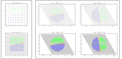
Figure IV.1: Depiction of representative real-space partitions used in our lattice simulation to produce Fig. 3 in the main text. Left panel for the square lattice, and right panel for the triangular lattice with both $x$- and $y$-partition shown. Sites colored in gray belong to region $E$, which are not used in the computation. The remaining four colored regions $A,B,C,D$ are used, with total linear size $2L/3$. This strategy allows us to suppress unwanted contribution from gapless boundary modes which exist in a topological phase. One-dimensional gapless modes generally contribute a logarithmic divergence (in the size of the boundary interval where it lives in), and cannot be properly canceled out in the combination in Eq. (6).

For convenience of interested readers, here we specify explicitly the real-space lattice Hamiltonian and illustrate some representative real-space partition configurations we use for obtaining the results shown in Fig. 3 of the main text. In this work we have studied three lattice models with open boundary conditions. For the Harper-Hofstadter (HH) model with $2\pi/q$-flux per plaquette Harper (1955); Hofstadter (1976), we have

$$H_{HH}=\sum_{{\bf R}}\big{(}e^{i\frac{2\pi{\bf R}_{x}}{q}}c^{\dagger}_{{\bf R}+\hat{y}}c_{\bf R}+c^{\dagger}_{{\bf R}+\hat{x}}c_{\bf R}\big{)}+\text{H.c.},$$ (IV.9)

where $c^{\dagger}_{\bf R}$ is the fermionic creation operator at site ${\bf R}$ on a square lattice. For the Qi-Wu-Zhang (QWZ) model Qi et al. (2006) on a square lattice with two orbitals (labeled $1$ and $2$) per site, we have

$$\begin{split}H_{QWZ}=\sum_{\bf R}\Big{\{}&-\frac{t_{y}}{2}(c^{\dagger}_{{\bf R}+\hat{y},2}c_{{\bf R},1}-c^{\dagger}_{{\bf R}+\hat{y},1}c_{{\bf R},2}+c^{\dagger}_{{\bf R}+\hat{y},1}c_{{\bf R},1}-c^{\dagger}_{{\bf R}+\hat{y},2}c_{{\bf R},2})\\ &-\frac{t_{x}}{2}(c^{\dagger}_{{\bf R}+\hat{x},1}c_{{\bf R},1}-c^{\dagger}_{{\bf R}+\hat{x},2}c_{{\bf R},2}-ic^{\dagger}_{{\bf R}+\hat{x},2}c_{{\bf R},1}-ic^{\dagger}_{{\bf R}+\hat{x},1}c_{{\bf R},2})\\ &+\frac{M}{2}(c^{\dagger}_{{\bf R},1}c_{{\bf R},1}-c^{\dagger}_{{\bf R},2}c_{{\bf R},2})\Big{\}}+\text{H.c.}.\end{split}$$ (IV.10)

We have studied both the isotropic case with $t_{x}=t_{y}=t$ and the anisotropic case with $t_{x}=2t_{y}=t$ in the main text. Lastly, we have the Haldane model Haldane (1988) on the triangular lattice with two orbitals (labeled $1$ and $2$) per site. Notice the orbital-embedding we use here is different from the honeycomb model that Haldane proposed originally. The difference is in the real-space position of orbitals, which does not affect the energy spectrum but would indeed affect the quantum geometry of bands. We thus remark on this point here, as it is the quantum geometry that concerns us in this work. Denoting the three $C_{3}$-related primitive vectors as ${\bf a}_{i=1,2,3}$, we have

$$\begin{split}H_{H}=&\sum_{{\bf R}}\Big{\{}\;t(c^{\dagger}_{{\bf R},2}c_{{\bf R},1}+c^{\dagger}_{{\bf R}-{\bf a}_{3},2}c_{{\bf R},1}+c^{\dagger}_{{\bf R}+{\bf a}_{2},2}c_{{\bf R},1})\\ &+t^{\prime}\Big{[}\big{(}e^{-i\phi}\sum_{i=1}^{3}c^{\dagger}_{{\bf R}+{\bf a}_{i},1}c_{{\bf R},1}\big{)}+\big{(}1\rightarrow 2,\;\phi\rightarrow-\phi\big{)}\Big{]}+\frac{M}{2}(c^{\dagger}_{{\bf R},1}c_{{\bf R},1}-c^{\dagger}_{{\bf R},2}c_{{\bf R},2})\;\Big{\}}+\text{H.c.}.\end{split}$$ (IV.11)

In the main text, we have focused on $t^{\prime}=0.3t$ and $\phi=\pi/2$. In Sec. III we have also studied the Haldane honeycomb model (which is the original version proposed in Ref. Haldane (1988)), with the same form of Hamiltonian but now orbitals 1 and 2 are spatially separated on the sites of the honeycomb lattice, as depicted in Fig. III.1(b).

Finally, we have shown in Fig. IV.1 some of the real-space partition configurations that we have used for the numerical simulation of corner fluctuation and corner entanglement entropies.