1 Introduction

A promising strategy for understanding fundamental interactions relies on studying the consistency conditions of scattering amplitudes. This approach seeks to determine which theories adhere to foundational principles that are stringent enough to filter out most candidates, yet permissive enough to accommodate a few (or unique) viable scattering amplitudes. This line of reasoning has proven very fruitful in the context of relativistic quantum scattering in Minkowski space, particularly for massless particles with spin.

For instance, it is well-established that any theory describing massless spin-1 particles must be a gauge theory while the theory of a massless spin-2 particle is unique in its infrared limit, corresponding to general relativity (GR) [1, 2]. Similarly, the theory of massless spin-3/2 particles must be a supergravity theory [3], while massless particles with spins greater than 2 have a trivial $S$-matrix [4], a result extending the Weinberg-Witten constraints on massless particles [5]. In recent years, positivity bounds and $S$-matrix bootstrap constraints have further shaped the landscape of consistent theories, extending some of the previous results to massive spinning particles, see e.g. [6, 7, 8, 9].

In a sense, these constraints can be viewed as modern selection rules derived directly from the fundamental principles of quantum mechanics and relativity.

However, amidst this well-explored landscape, there exists a class of massless particles that has received considerably less attention: continuous-spin particles (CSPs). CSPs are massless irreducible unitary representations (irreps) of the Poincaré group, classified long ago by Wigner [10]. As the associated little group (LG) is non-compact and faithfully represented, a CSP carries infinitely many degrees of freedom even at fixed momentum.

The theory of CSPs has been found incompatible with the stringent axioms of local field theory, see e.g. [11, 12, 13]. However, it was realized years later that the assumptions could be significantly relaxed, as the axiomatic approach would otherwise reject ordinary gauge and gravity theories. A free Lagrangian gauge-theory formulation emerged [14, 15, 16, 17] along with some encouraging results extracted from soft limits of the scattering amplitudes. This progress triggered further investigations, such as e.g. [19, 20, 21, 22, 23], and an interacting Lagrangian theory, formulated in terms of gauge fields coupled to matter worldlines, has been recently proposed [18, 24].

Stimulated by these intriguing advances, the purpose of this paper is twofold: (i) to understand the properties of CSPs directly through the lens of consistency conditions of on-shell scattering amplitudes; (ii) to explore which principles — if any — need to be relaxed for non-trivial solutions of the constraints to exist. A vital part of both points is also the derivation of explicit amplitudes that bear direct physical implications of underlying principles.

This on-shell approach is particularly well-suited to analyze CSP dynamics and scrutinize its unusual features in a very transparent way. Indeed, it allows us to classify all three-point one-shell amplitudes consistent with LG-covariance, analyticity, and well-defined high-energy behavior. We characterize as well the structure of all on-shell $n-$point amplitudes, and analyse their properties concerning on-shell factorisation —extended unitarity—, analyticity, crossing symmetry, and high-energy limits. We illustrate our findings through several examples. We finally critically discuss possible ways to relax these constraints and their implications for gravity and electromagnetism.

The paper is structured as follows: Section 2 introduces basic kinematic concepts and defines CSPs. In Section 3, we present the primary findings of this study, bootstrapping amplitudes for CSPs from foundational principles. Section 4 showcases non-trivial examples that highlight key features of CSPs amplitudes, while Section 5 explores the relaxation of certain constraints and their resulting physical implications. Finally, we summarize our findings and explore future directions in Section 6.

2 Kinematics and Poincaré

We consider a relativistic quantum theory of particles scattering in four-dimensional Minkowski space. We assume the dynamics is invariant under the inhomogeneous proper Lorentz group. In particular asymptotic in- and out-going scattering states not only cover the entire positive Hilbert space —unitarity— but also transform as the tensor product of single particle states which carry themselves a unitary irrep. Each particle $i=1,2,\ldots$ is thus associated to a pair of real numbers $(m^{2}_{i},\mu^{2}_{i})$ which are the values taken by the two Casimir operators —the mass-squared and the Pauli-Lubanski squared—

$$P_{\mu}P^{\mu}=m^{2}\ ,\qquad W_{\mu}W^{\mu}=-\mu^{2}\ .$$ (2.1)

The Casimirs are written in terms of the group generator $P^{\mu}$ and $J^{\mu\nu}$, and the so-called Pauli-Lubanski pseudo-vector

$$W_{\mu}\equiv\frac{1}{2}\epsilon_{\mu\nu\rho\sigma}J^{\nu\rho}P^{\sigma}\ ,\qquad[W_{\mu},P_{\mu}]=0\ ,\qquad[W_{\mu},W_{\nu}]=-i\epsilon_{\mu\nu\rho\sigma}W^{\rho}P^{\sigma}\ .$$ (2.2)

On a subspace spanned by definite-momentum states with $p^{\mu}\neq 0$, the (2.2) imply that the Pauli-Lubanski is the generator of the “little group” $H^{p}$ of $p^{\mu}$, that is the Lorentz subgroup that leaves that definite-$p^{\mu}$ subspace invariant.

For a null momentum $p^{2}=0$, the $H^{p}\sim ISO(2)$, which is the group of isometries of 2D euclidean plane made of rotations $\mathbb{H}$ around the direction of motion —the helicity— and translations $\mathbb{W}^{\pm}$

$$[\mathbb{H},\mathbb{W}^{\pm}]=\pm\mathbb{W}^{\pm}\ ,\qquad[\mathbb{W}^{+},\mathbb{W}^{-}]=0\ .$$ (2.3)

For instance, the $ISO(2)=H^{\widehat{p}}$ generators associated to $p=\widehat{p}=(1,0,0,1)$ are $\mathbb{H}=J_{3}=-W_{3}$ and $\mathbb{W}^{\pm}=-(W_{1}\pm iW_{2})$. The latter are lowering and raising operators within the complexified Lorentz algebra $sl(2,\mathbb{C})\times sl(2,\mathbb{C})$. For a massive momentum $p^{2}>0$, the little group is the familiar rotation group $SU(2)$.

The little group $H^{p}$ is relevant because unitary irreps $D(g)$ of its universal cover, $|p\,h\rangle\to|p\,h^{\prime}\rangle D_{h^{\prime}}^{\,\,h}(g)$, induce unitary irreps of the $SL(2,\mathbb{C})$, on generic momentum state

$$|k\,h\rangle\to|\Lambda k\,h^{\prime}\rangle D^{h^{\prime}}_{\,\,h}(W(\Lambda,p,k))\ ,\qquad W(\Lambda,p,k)\in H^{p}$$ (2.4)

where the Wigner transformation $W(\Lambda,p,k)$ depends in some complicated way on the chosen reference momentum $p$, the momentum $k$ of the state, and the conventional choice of Lorentz transformation $L(p,k):p\to k$ used to define the state $|k\,h\rangle\equiv U(L(p,k))|p\,h\rangle$. Different choices of $p$ or $L(p,k)$ correspond to redefining the states by a little-group transformation in $H^{p}$, $H^{k}$, or their intersection (pairwise helicity transformations). These ambiguities, which reflect the freedom of choosing the basis for each one-particle state independently, manifest themselves in the little-group covariance of scattering amplitudes with respect to each $H^{p_{i}}$. Then, in the following, we assume that amplitudes provide a linear space where the tensor product representation $\bigotimes_{i}D_{i}$ acts, where the sub-index $i$ distinguishes the irreps for the $i-th$ particle.

The states of definite $p$ for a single CSP can be labelled by diagonalising the helicity $\mathbb{H}$ — the $h$-basis — where

$$\mathbb{H}|p\,h\rangle=h|p\,h\rangle\ ,\qquad\mathbb{W}^{\pm}|p\,h\rangle=\mu|p\,h\pm 1\rangle$$ (2.5)

so that rotations multiply by a phase whereas translations mix all helicity by a Bessel function $D\sim J_{h-h^{\prime}}$. Notice that the helicity is no longer Lorentz invariant as $\mathbb{W}_{\pm}$ can raise/lower it. It is still taking nevertheless (all) integers or (all) half-integers values.

In the rest of the paper we find it easier to work in a basis that diagonalises both $\mathbb{W}^{\pm}$ — the $\theta$ basis —

$$\mathbb{W}^{\pm}|p\,\theta\rangle=\mu^{\pm}|p\,\theta\rangle\ ,\qquad\mathbb{H}|p\,\theta\rangle=i\frac{\partial}{\partial\theta}|p\,\theta\rangle\ ,\qquad\mu^{\pm}\equiv\mu e^{\pm i\theta}$$ (2.6)

where the state is defined by an angle $\theta$ with $2\pi$ ($4\pi$) periodicity for bosons (fermions). The $ISO(2)$-translations act multiplicatively, whereas the helicity is rotating $\theta$

$$e^{i\alpha^{+}\mathbb{W}^{-}+i\alpha^{-}\mathbb{W}^{+}}|p\,\theta\rangle=e^{i\alpha^{+}\mu^{-}+i\alpha^{-}\mu^{+}}|p\,\theta\rangle\ ,\qquad e^{-i\omega\mathbb{H}}|p\,\theta\rangle=|p\,\theta+\omega\rangle\ .$$ (2.7)

The $\theta$ and helicity-basis are connected by a simple Fourier transform:

$$\begin{split}|p\,h\rangle=\int_{0}^{2\pi}\!\frac{\differential\theta}{2\pi}\,e^{+i\theta h}\,|p\,\theta\rangle=\int_{0}^{2\pi}\!\frac{\differential\theta}{2\pi}\,e^{+i\theta h}\sum_{\bar{h}=-\infty}^{+\infty}e^{-i\theta\bar{h}}|p^{\mu}\,\bar{h}\rangle\ .\end{split}$$ (2.8)

In the following, we assume the S-matrix operator commutes with translations and Lorentz generators, $[S,P^{\mu}]=0=[S,J^{\mu\nu}]$. The first equality implies momentum conservation in the form of an overall Dirac-delta in the scattering amplitudes

$$i(2\pi)^{4}\delta^{4}(\sum k_{i})\mathcal{M}_{h_{1}\ldots h_{n}}(k_{1},\ldots k_{n})=\langle\mathrm{out}|S-\mathbb{I}|\mathrm{in}\rangle\ .$$ (2.9)

Moreover, Lorentz invariance demands the following relation

$$\mathcal{M}_{h_{1}\ldots h_{n}}(k_{1},\ldots k_{n})=\mathcal{M}_{h^{\prime}_{1}\ldots h^{\prime}_{n}}(\Lambda k_{1},\ldots\Lambda k_{n}){D_{1}}^{h^{\prime}_{1}}_{\,\,h_{1}}(W(\Lambda,p,k_{1}))\cdots{D_{n}}^{h^{\prime}_{n}}_{\,\,h_{n}}(W(\Lambda,p,k_{1}))\ .$$ (2.10)

In particular, $D_{i}=D^{(\mu_{i})}$ for a in-state CSP, and its complex conjugate irrep $D_{i}=D^{*(\mu_{i})}$ for a out-state CSP instead. The distinction between incoming and outgoing irreps is in fact artificial. For instance, ordinary massless particles in the out-state transform like in-states of opposite helicity. CSPs in the out-state transform as in-state CSPs up to the replacement $\theta\to\theta+\pi$, schematically $\langle p\,\,\theta|\sim|p\,\,\theta+\pi\rangle$ (or $\langle p\,\,h|\to(-1)^{h}|p\,\,-\!h\rangle$). Analogous story for massive particles.

Without loss of generality, we thus adopt an all-in convention where particles transform as if they were all in-states.

3 Bootstrapping Amplitudes

3.1 $ISO(2)$ functionals

Little group covariance and Lorentz invariance (2.10) are the kinematic constraints on amplitudes studied in this section. Ordinary massless and massive amplitudes solve these constraints because they are $SL(2,\mathbb{C})\times SL(2,\mathbb{C})$-invariant functions of spinors. Indeed, given a particle of null momentum, the associated spinors

$$|p\rangle[p|=\lambda_{\alpha}\lambda_{\dot{\alpha}}=p_{\alpha\dot{\alpha}}\ ,\qquad p^{2}=0$$ (3.1)

are defined only up to (complexified) little group transformations, as rescaling $\lambda(p)\to w\lambda(p)_{\alpha}$ and $\lambda_{\dot{\alpha}}(p)\to w^{-1}\lambda(p)_{\alpha}$ preserves the momentum. They are elements of an equivalence class $(p^{\mu},p^{2}=0)\leftrightarrow(|p\rangle,|p])/U(1)$. Acting with a $SL(2,\mathbb{C})\times SL(2,\mathbb{C})$ transformation on a conventionally chosen representative of the element class maps into another choice

$$\Lambda_{\alpha}^{\,\,\beta}\lambda_{\beta}(p)=w\lambda_{\beta}(\Lambda p)\ ,\qquad\Lambda_{\dot{\alpha}}^{\,\,\dot{\beta}}\lambda_{\dot{\beta}}(p)=w^{-1}\lambda_{\dot{\beta}}(\Lambda p)\ .$$ (3.2)

Therefore, amplitudes of the form $\mathcal{M}_{h_{1}\ldots h_{n}}(\{|i\rangle,|i]\})=\mathcal{M}\left(\langle ij\rangle,[ij]\right)$ satisfy the Lorentz invariant constraint (2.10) if

$$\mathcal{M}_{h_{1}\ldots h_{n}}(\{w_{i}|i\rangle,w_{i}^{-1}|i]\})=\left(w_{i}\right)^{2h_{i}}\times\mathcal{M}_{h_{1}\ldots h_{n}}(\{|i\rangle,|i]\})\qquad\forall i=1,\ldots n\ .$$ (3.3)

But this is precisely the $U(1)$ little-group covariant constraint, the only one left to enforce for ordinary massless particles. It is rather simple because it amounts to counting left-handed and right-handed spinors for each particle. This counting can be translated into an equivalent differential problem

$$\mathbb{H}_{i}\mathcal{M}_{h_{1}\ldots h_{n}}=h_{i}\mathcal{M}_{h_{1}\ldots h_{n}}\qquad\mathbb{H}_{i}=-\frac{1}{2}\left(|i\rangle\frac{\partial}{\partial|i\rangle}-|i]\frac{\partial}{\partial|i]}\right)\ .$$ (3.4)

The main lesson is that Lorentz invariant amplitudes are solutions of a linear differential problem defined by the little group of each particle. A completely analogous story can be told for massive spinors, see e.g. [25].

We apply now the same logic to CSPs. We need to find three differential operators $\mathbb{H}$, $\mathbb{W}^{\pm}$ that realise the $ISO(2)$ algebra (2.3) on the space of functions of spinors.

The space should be larger than the one considered above, or else $W_{\mu}^{2}=0$. Indeed, the translations operators act multiplicatively on it via $P_{\alpha\dot{\alpha}}=\lambda_{\alpha}\lambda_{\dot{\alpha}}$, while the little group is a Lorentz subgroup generated for each particle spinor by $J_{\alpha\beta}=i\lambda_{(\alpha}\frac{\partial}{\partial\lambda^{\beta)}}$ and $J_{\dot{\alpha}\dot{\beta}}=i\lambda_{(\dot{\alpha}}\frac{\partial}{\partial\lambda^{\dot{\beta})}}$. Using these expressions in the definition (2.2) of Pauli-Lubanski (in spinorial form) returns vanishing Casimirs

$$W_{\alpha\alpha}=\frac{-i}{2}\left(J_{\alpha}^{\,\,\beta}P_{\beta\dot{\alpha}}-J^{\dot{\beta}}_{\,\,\dot{\alpha}}P_{\alpha\dot{\beta}}\right)\longrightarrow W_{\alpha\beta}=P_{\alpha\dot{\alpha}}\mathbb{H}\longrightarrow W_{\alpha\dot{\alpha}}W^{\alpha\dot{\alpha}}=0\ ,$$ (3.5)

so that a functions of $(\lambda_{\alpha},\lambda_{\dot{\alpha}})$-only can’t describe a CSP.

A large enough space of functions of spinors is instead the one that acts on spinors $\lambda_{\alpha}$ and $\lambda_{\dot{\alpha}}$ defined by (3.1) as well as on linearly independent spinors denoted by $\rho_{\alpha}$ and $\rho_{\dot{\alpha}}$

$$\langle\lambda^{i}\rho^{i}\rangle=\langle i\mathmybb{i}\rangle\neq 0\ ,\qquad[\lambda^{i}\rho^{i}]=[i\mathmybb{j}]\neq 0\ .$$ (3.6)

We refer to these linear independent spinors as “black-board” angle (square) spinors $|\mathmybb{i}\rangle$ ($|\mathmybb{i}]$). They always exist because the space of spinors $\mathbb{C}^{2}$ is two-dimensional. Notice that the spinors are now nicely defined up to $ISO(2)$ transformations

$$|i\rangle\to w|i\rangle\ ,\quad|\mathmybb{i}\rangle\to w^{-1}|\mathmybb{i}\rangle+a|i\rangle\ ,\quad|i]\to w^{-1}|i]\ ,\quad|\mathmybb{i}]\to w|\mathmybb{i}]+b|i]\ ,$$ (3.7)

which leave invariant (3.1) and (3.6).

While translations are still realized by multiplication $P_{\alpha\dot{\alpha}}=\lambda_{\alpha}\lambda_{\dot{\alpha}}$ on this space, the Lorentz generators (for each particle) are

$$J_{\alpha\beta}=i\lambda_{(\alpha}\frac{\partial}{\partial\lambda^{\beta)}}+i\rho_{(\alpha}\frac{\partial}{\partial\rho^{\beta)}}\ ,\quad J_{\dot{\alpha}\dot{\beta}}=i\lambda_{(\dot{\alpha}}\frac{\partial}{\partial\lambda^{\dot{\beta})}}+i\rho_{(\dot{\alpha}}\frac{\partial}{\partial\rho^{\dot{\beta})}}\ ,$$ (3.8)

so that Pauli-Lubanski squared is the following functional:

$$\left(W_{\mu}W^{\mu}\right)_{i}=\frac{1}{2}\left(W_{\alpha\dot{\alpha}}W^{\alpha\dot{\alpha}}\right)_{i}=-\langle\lambda^{i}\rho^{i}\rangle[\lambda^{i}\rho^{i}]\lambda^{i}_{\alpha}\frac{\partial}{\partial\rho^{i}_{\alpha}}\lambda^{i}_{\dot{\alpha}}\frac{\partial}{\partial\rho^{i}_{\dot{\alpha}}}=-\langle i\mathmybb{i}\rangle[i\mathmybb{i}]\,|i\rangle\frac{\partial}{\partial|\mathmybb{i}\rangle}|i]\frac{\partial}{\partial|\mathmybb{i}]}\ ,$$ (3.9)

acting on the space of functions of bi-spinors. We recall that $W_{\mu}^{2}=-\mathbb{W}_{+}\mathbb{W}_{-}$. Thus, the differential operators $\mathbb{W}_{\pm}$, $\mathbb{H}$ acting on this space are easily extracted

$$\mathbb{W}^{-}_{i}=\langle i\mathmybb{i}\rangle|i\rangle\frac{\partial}{\partial|\mathmybb{i}\rangle}\ ,\qquad\mathbb{W}^{+}_{i}=[i\mathmybb{i}]|i]\frac{\partial}{\partial|\mathmybb{i}]}\ ,\qquad\mathbb{H}_{i}=-\frac{1}{2}\left(|i\rangle\frac{\partial}{\partial|i\rangle}-|\mathmybb{i}\rangle\frac{\partial}{\partial|\mathmybb{i}\rangle}-|i]\frac{\partial}{\partial|i]}+|\mathmybb{i}]\frac{\partial}{\partial|\mathmybb{i}]}\right)\ .$$ (3.10)

Indeed, they satisfy the $ISO(2)$ algebra (2.3). The $\mathbb{W}^{-}$ lowers $\rho_{\alpha}\to\propto\lambda_{\alpha}$, whereas $W^{+}$ raises $\rho^{\dot{\alpha}}\to\propto\lambda^{\dot{\alpha}}$, and have helicity $\mp$ respectively. Labelling explicitly the amplitudes by $\theta_{i}$-angles associated with the states, the amplitudes must solve

$$\mathbb{W^{\pm}}_{i}\mathcal{M}_{\theta_{1}\ldots\theta_{n}}=\mu_{i}^{\pm}\mathcal{M}_{\theta_{1}\ldots\theta_{n}}\ ,\qquad\mathbb{H}_{i}\mathcal{M}_{\theta_{1}\ldots\theta_{n}}=i\frac{\partial}{\partial\theta_{i}}\mathcal{M}_{\theta_{1}\ldots\theta_{n}}\ ,\qquad\forall i=1,\dots,n\ .$$ (3.11)

Finally, since amplitudes are functions of invariant contractions only, these equations are equivalent to the following set of differential equations:

$$\langle i\mathmybb{i}\rangle\sum_{j=1}^{n}\left(\langle ji\rangle\frac{\partial}{\partial\langle j\mathmybb{i}\rangle}+\langle\mathmybb{j}i\rangle\frac{\partial}{\partial\langle\mathmybb{j}\mathmybb{i}\rangle}+\ldots\right)\log\mathcal{M}_{\theta_{1}\ldots\theta_{n}}=\mu^{-}_{i}\ ,$$ (3.12a)

$$[i\mathmybb{i}]\sum_{j=1}^{n}\left([ji]\frac{\partial}{\partial[j\mathmybb{i}]}+[\mathmybb{j}i]\frac{\partial}{\partial[\mathmybb{j}\mathmybb{i}]}+\ldots\right)\log\mathcal{M}_{\theta_{1}\ldots\theta_{n}}=\mu^{+}_{i}\ ,$$ (3.12b)

$$\mathrm{Exp}\left(-i\omega\mathbb{H}_{i}\right)\mathcal{M}_{\theta_{1}\ldots\theta_{n}}=\mathcal{M}_{\theta_{1}\ldots(\theta_{i}+\omega)\ldots\theta_{n}}\ ,$$ (3.12c)

where we explicitly display differentiation w.r.t. massless spinors while ellipsis contain as well derivatives w.r.t. massive spinors, such as e.g. $\langle\boldsymbol{j}^{I}i\rangle\frac{\partial}{\partial\langle\boldsymbol{j}^{I}\mathmybb{i}\rangle}$ for $\mathbb{W}_{-}$, whenever present. The amplitudes in these differential equations are functions of massless and massive spinors that may appear in the problem

$$\mathcal{M}_{\theta_{1}\ldots\theta_{n}}=\mathcal{M}_{\theta_{1}\ldots\theta_{n}}\left(\langle ij\rangle,\langle i\mathmybb{j}\rangle,\langle\mathmybb{i}\mathmybb{j}\rangle,\langle\boldsymbol{i}j\rangle,\langle\boldsymbol{i}\mathmybb{j}\rangle,\langle\boldsymbol{i}{j}\rangle,[ij],[\mathmybb{i}j],\ldots\right)\ ,$$ (3.13)

but typically momentum conservation, on-shell conditions, and Schouten identities reduce the number of independent contractions to be considered.

We observe that the space of functions of spinors can actually be larger than the one we considered so far. It can contain as well complex conjugate spinors that carry complex conjugate irreps, within the complexified Lorentz group $SL(2,\mathbb{C})\times SL(2,\mathbb{C})$. We study amplitudes resulting from this extended space of functions in Section 5.5. Until then, we restrict to functions that are analytic in the spinors.

3.2 Three-point Amplitudes

In this section, we present first some simple fully worked-out solutions to the kinematic constraints (3.12) for three-point amplitudes involving CSPs, in preparation for the general $n$-point amplitude presented in the next sections.

3.2.1 2-CSP and 1 massive spin-$j$

This simple example covers several of the interesting general features that CSP amplitudes display. It is moreover interesting on its own to extract the partial-wave (PW) expansion [26] of a general 4-CSP amplitude, as it can be interpreted as the Poincaré Clebsh-Gordan coefficients (CGCs) for amplitudes with external CSPs, following [25, 27, 28]. This is discussed in Section 4.4.

We assign particles $i=1,2$ to be CSPs, and $i=3$ the particle of mass $m=m_{3}$. Momentum conservation $|\mathbf{3}^{I}\rangle[\mathbf{3}_{I}|=-|1\rangle[1|-|2\rangle[2|$, on-shell conditions $\langle 12\rangle[21]=m_{3}^{2}$, and the Schouten identities tell that the only non-trivial and independent contractions transforming under $ISO(2)$ are $\langle\mathmybb{1}2\rangle$, $\langle\mathmybb{2}1\rangle$, $[\mathmybb{1}2]$, $[\mathmybb{2}1]$, and either one between $\langle ij\rangle$ and $[ij]$. Therefore, the first two differential equations $W^{\pm}_{i}\mathcal{M}=\mu^{\pm}_{i}$ for $i=1,2$ in (3.12a) and (3.12b) greatly simplify to

$$\langle 21\rangle\frac{\partial}{\partial\langle 2\mathmybb{1}\rangle}\log\mathcal{M}_{\theta_{1}\theta_{2}}=\frac{\mu^{-}_{1}}{\langle 1\mathmybb{1}\rangle}\ ,\qquad[21]\frac{\partial}{\partial[2\mathmybb{1}]}\log\mathcal{M}_{\theta_{1}\theta_{2}}=\frac{\mu^{+}_{1}}{[1\mathmybb{1}]}\ ,$$ (3.14a)

$$\langle 12\rangle\frac{\partial}{\partial\langle 1\mathmybb{2}\rangle}\log\mathcal{M}_{\theta_{1}\theta_{2}}=\frac{\mu^{-}_{2}}{\langle 2\mathmybb{2}\rangle}\ ,\qquad[12]\frac{\partial}{\partial[1\mathmybb{2}]}\log\mathcal{M}_{\theta_{1}\theta_{2}}=\frac{\mu^{+}_{2}}{[2\mathmybb{2}]}\ .$$ (3.14b)

Their solutions are

$$\begin{split}\mathcal{M}_{\theta_{1}\theta_{2}}=\exp\left(\frac{\mu_{1}^{-}}{\langle 1\mathmybb{1}\rangle}\frac{\langle 2\mathmybb{1}\rangle}{\langle 21\rangle}+\frac{\mu_{1}^{+}}{[1\mathmybb{1}]}\frac{[2\mathmybb{1}]}{[21]}\right)\exp\left(\frac{\mu_{2}^{-}}{\langle 2\mathmybb{2}\rangle}\frac{\langle 1\mathmybb{2}\rangle}{\langle 12\rangle}+\frac{\mu_{2}^{+}}{[2\mathmybb{2}]}\frac{[1\mathmybb{2}]}{[12]}\right)\widetilde{\mathcal{M}}_{\theta_{1}\theta_{2}}\ ,\end{split}$$ (3.15)

where $\widetilde{\mathcal{M}}_{\theta_{1}\theta_{2}}$ is a function of ordinary massless and massive spinors, dependent on $\theta_{i=1,2}$ (and possibly on the $\mu_{i}$ and/or other constants).

The final constraint from the helicity equation (3.12c) is trivially solved by the exponential prefactors in (3.15), e.g. $\mu e^{-i\theta_{1}}\langle 2\mathmybb{1}\rangle/\langle 21\rangle\to\mu e^{-i(\theta_{1}+\omega)}\langle 2\mathmybb{1}\rangle/\langle 21\rangle$ under $\mathrm{Exp(-i\omega\mathbb{H}_{1})}$, because $|\mathmybb{i}\rangle$ and $|i\rangle$ have helicities $+1/2$ and $-1/2$, respectively. The remaining non-trivial constraint imposed by (3.12c) on $\widetilde{\mathcal{M}}_{\theta_{1}\theta_{2}}$ can be solved in a similar vein, namely

$$\widetilde{\mathcal{M}}_{\theta_{1}\theta_{2}}=\sum_{\{h_{i}\}}\mathcal{M}_{h_{1}h_{2}}e^{-ih_{1}\theta_{1}-ih_{2}\theta_{2}}\ ,$$ (3.16)

where $\mathcal{M}_{h_{1}h_{2}}=\mathcal{M}_{h_{1}h_{2}}(|i\rangle,|j],|\mathbb{3}\rangle,|\mathbb{3}])$ are ordinary three-point amplitudes between two (ordinary) massless particles of helicity $h_{i=1,2}$ and a massive particle of spin-$j$. These are completely classified, see e.g. [25], and therefore the problem is fully solved, see (3.19).

Finally, we highlight two features that are discussed in full generality in the following: i) the massless limit $m\to 0$ where all particles are degenerate is singular because $\langle 12\rangle[21]=m^{2}$; ii) the high-energy limit of CSPs just returns $\mathcal{M}_{\theta_{1}\theta_{2}}\to\widetilde{\mathcal{M}}_{\theta_{1}\theta_{2}}$, which Fourier-transformed back to helicity-basis gives the ordinary amplitudes $\mathcal{M}_{h_{1}h_{2}}$ in (3.16). Therefore, one can think of the three-point amplitude (3.15) as the IR deformation of a UV theory that had only ordinary massless particles of helicity $h_{i}$ in the three-point amplitude, with infinitely many helicities recoupling-in as the momenta are lowered down to $\mu$. For instance, choosing

$$\mathcal{M}_{h_{1}h_{2}}=\delta_{h_{1}}^{-1}\delta_{h_{2}}^{-1}\langle 12\rangle^{2}/f_{-}+\delta_{h_{1}}^{1}\delta_{h_{2}}^{1}[12]^{2}/f_{+}$$ (3.17)

corresponds to two CSPs coupled to a massive scalar $j=0$, in a way that at high energy only helicities $\pm 1$ remain coupled, with strenght set by decay constants $f_{\pm}$. That is the high-energy limit is the same as produced by (a linear combination of) field theory interactions $F_{\mu\nu}F^{\mu\nu}\phi$ and $F_{\mu\nu}\widetilde{F}^{\mu\nu}\phi$ for higgs-like and/or axion-like particles.

Another example is the coupling of two CSPs that in the high-energy limit reduces to the “minimal coupling” of $\pm 1$-helicity photons coupled to a massive $j=2$ particle, corresponding to the choice

$$\mathcal{M}_{h_{1}h_{2}}=\delta_{h_{1}}^{-1}\delta_{h_{2}}^{+1}\frac{\langle 1\boldsymbol{3}\rangle^{4}}{\langle 12\rangle^{2}}/f_{-}+\delta_{h_{1}}^{+1}\delta_{h_{2}}^{-1}\frac{[1\boldsymbol{3}]^{4}}{[12]^{2}}/f_{+}\ ,$$ (3.18)

where the interaction strength is set by decay constants $f_{\pm}$. In a parity preserving theory $f_{-}=f_{+}$ and this is what it is obtained by coupling a massive spin-2 particle to the photon energy-momentum tensor.

The resulting general amplitude that is useful e.g. for the PW-decomposition is reported here for later convenience:

$$\mathcal{M}_{\theta_{1}\theta_{2}}= \exp\left(\frac{\mu_{1}^{-}}{\langle 1\mathmybb{1}\rangle}\frac{\langle 2\mathmybb{1}\rangle}{\langle 21\rangle}+\frac{\mu_{1}^{+}}{[1\mathmybb{1}]}\frac{[2\mathmybb{1}]}{[21]}\right)\exp\left(\frac{\mu_{2}^{-}}{\langle 2\mathmybb{2}\rangle}\frac{\langle 1\mathmybb{2}\rangle}{\langle 12\rangle}+\frac{\mu_{2}^{+}}{[2\mathmybb{2}]}\frac{[1\mathmybb{2}]}{[12]}\right)\widetilde{M}_{\theta_{1}\theta_{2}}\ ,$$ (3.19a)

$$\widetilde{M}_{\theta_{1}\theta_{2}}= c_{j}\sum_{h_{1}h_{2}}\frac{e^{-i\theta_{1}h_{1}-ih_{2}\theta_{2}}}{m^{2j+h_{1}+h_{2}-1}}\langle 1\boldsymbol{j}\rangle^{j+h_{2}-h_{1}}\langle 2\boldsymbol{j}\rangle^{j+h_{1}-h_{2}}[12]^{j+h_{1}+h_{2}}\ .$$ (3.19b)

3.2.2 1-CSP, 1 massless particle and 1 massive spin-$j$

This example is a simple variation of the case study in previous Section 3.2.1 where now one of the two $\mu_{i}$ is set to zero, for instance $\mu_{2}=0$. For this reason, we highlight only its main steps.

Particle 1 is the CSP, particle 2 is the ordinary massless particle of helicity $h_{2}$, while particle 3 has mass $m=m_{3}$. We can choose the non-trivial contractions with the black-board spinors to be $\langle\mathmybb{1}2\rangle$ and $[\mathmybb{1}2]$. The differential equations (3.12a) and (3.12b) for $\mathbb{W}^{\pm}$ reduce again to just (3.14a). Mutatis mutandis the solution is

$$\mathcal{M}_{\theta_{1}}=\exp\left(\frac{\mu_{1}^{-}}{\langle 1\mathmybb{1}\rangle}\frac{\langle 2\mathmybb{1}\rangle}{\langle 21\rangle}+\frac{\mu_{1}^{+}}{[1\mathmybb{1}]}\frac{[2\mathmybb{1}]}{[21]}\right)\left(\sum_{h_{i}}\mathcal{M}_{h_{1}h_{2}}e^{-ih_{1}\theta_{1}}\right)$$ (3.20)

where again $\mathcal{M}_{h_{1}h_{2}}=\mathcal{M}_{h_{1}h_{2}}(|i\rangle,|j],|\mathbb{3}\rangle,|\mathbb{3}])$ are ordinary three-point amplitudes between two (ordinary) massless particles of helicity $h_{i=1,2}$ and a massive particle of spin-$j$. These are classified and the problem is fully solved. Notice again that the high-energy limit is trivially set by $\mathcal{M}_{h_{1}h_{2}}$, and the massless limit $m_{3}\to 0$ is singular because momentum conservation and on-shell conditions demand $\langle 12\rangle[21]=m^{2}_{3}$.

We note that adding black-board spinors $|\mathmybb{2}\rangle$ and $|\mathmybb{2}]$ for ordinary massless particle 2 is just equivalent to repeat the example in Section 3.2.1 and take $\mu_{2}=0$. The solution collapses to (3.20) after Fourier transforming, effectively setting $\theta_{2}=0$. This is actually a general fact: adding black-board spinors to ordinary massless particles $j$ can not enlarge (non-trivially) the space of solutions. The reason is that from $\mathbb{W}^{\pm}_{j}\mathcal{M}=0$ it follows that the amplitude can at most carry the dependence on black-board spinors only via the choice of normalizations $\langle j\mathmybb{j}\rangle$ and $|j\mathmybb{j}]$.

3.2.3 1-CSP and 2 massive spin $j_{1}$, $j_{2}$

We choose for this example particle 3 as the CSP, while particles 1 and 2 carry spin $j_{1}$, $j_{2}$ and masses $m_{1}$, $m_{2}$. From playing with previous examples, it is not hard to guess the solution to the $ISO(2)$ functional problem (3.12), namely

$$\begin{split}\mathcal{M}_{\theta_{3}}=\exp\left(\frac{\mu^{+}_{3}}{[3\mathmybb{3}]}\frac{\langle 3|p_{1}|\mathmybb{3}]}{\langle 3|p_{1}|3]}+\frac{\mu^{-}_{3}}{\langle 3\mathmybb{3}\rangle}\frac{\langle\mathmybb{3}|p_{1}|3]}{\langle 3|p_{1}|3]}\right)\left(\sum_{h_{3}}\mathcal{M}_{h_{3}}e^{-ih_{3}\theta_{3}}\right)\ ,\end{split}$$ (3.21)

where $\mathcal{M}_{h_{3}}$ is again an ordinary amplitude between one massless particle of helicity $\{h_{3}\}$ and the two massive spinning particles. Its choice fixes the high-energy limit of the CSP to be the same as the one of a massless particle of helicity $h_{3}$ coupled to those spins. Finally, the limit where two particles are degenerate in mass is again singular because momentum conservation and on-shell condition enforce $m_{2}^{2}-m_{1}^{2}=\langle 3|p_{1}|3]\to 0$ and the amplitude has an essential singularity. We checked that there are no other solutions to the equations (3.12a) and (3.12b) in the case $m_{1}=m_{2}$ because the only independent contraction is $\langle\mathmybb{3}|p_{1}|\mathmybb{3}]$.

This amplitude may be used to describe the excitation of a composite particle or extended system that has more energy levels, through the absorption or the emission of CSPs.

3.2.4 3-CSP and the mass-splitting selection rule

The most striking observation of this subsection is that three-massless interactions with at least one CSP are always kinematically forbidden.

We remind the reader that three-point massless kinematics requires the vanishing of all Mandelstam invariants

$$s_{ij}=\langle ij\rangle[ji]=0\quad\forall(i,j)\ .$$ (3.22)

Complex momenta allow for a solution of this constraint where either

$$[ij]=0\quad\forall(i,j)\ ,\quad\text{or}\quad\langle ij\rangle=0\quad\forall(i,j)\ ,$$ (3.23)

to which we usually refer as holomorphic and anti-holomorphic configurations, respectively. While complex kinematics is enough for ordinary massless particles to admit non-trivial three-point amplitudes, this is not the case for CSPs. In order to show this, we consider a holomorphic configuration, such that the only non-vanishing square brackets are $[i\mathmybb{j}]$. Therefore, the $\mathbb{W}^{+}$-differential equations (3.12b) demand

$$\sum_{j\neq i}^{3}[\mathmybb{j}i]\frac{\partial}{\partial[\mathmybb{j}\mathmybb{i}]}\mathcal{M}_{\theta_{1}\ldots\theta_{n}}=\frac{\mu^{+}_{i}}{[i\mathmybb{i}]}\mathcal{M}_{\theta_{1}\theta_{2}\theta_{3}}\ ,\quad\forall i=1,2,3\ .$$ (3.24)

Enforcing momentum conservation and using $\langle ki\rangle[i\mathmybb{j}]+\langle kj\rangle[j\mathmybb{j}]=0$ for $i\neq j\neq k$, we can express $[i\mathmybb{j}]$ in terms of angle bracket and constant $[j\mathmybb{j}]$. The resulting system has no solutions unless all $\mu_{i}=0$. An equivalent argument applies to the anti-holomorphic configuration.

The same conclusion can be reached by guessing the solution (see also (3.27))

$$\prod_{i=1}^{3}\exp\left(\frac{\mu_{i}^{-}}{\langle i\mathmybb{i}\rangle}\frac{\langle\xi\mathmybb{i}\rangle}{\langle\xi i\rangle}+\frac{\mu_{i}^{+}}{[i\mathmybb{i}]}\frac{[\xi\mathmybb{i}]}{[\xi i]}\right)\widetilde{\mathcal{M}}\ ,$$ (3.25)

for some pair of spinors $|\xi\rangle$ and $|\xi]$. As soon as one requires these auxiliary spinors to be a non-vanishing linear combination of the spinors of the problem, and demand momentum conservation, either one between $[\xi i]$ or $\langle\xi i\rangle$ has to vanish, and so the solution diverges unless all $\mu_{i}=0$.

Taken at face value, this conclusion, along with the results of previous subsections, implies that no on-shell three-point amplitude exists (within the assumptions made) among at least one CSP and two other particles of degenerate mass. We refer to this condition as the “mass-splitting selection rule”.

The mass-splitting selection rule has interesting consequences:

1. No on-shell coupling of CSP to (massless) gravitons is possible. Similarly, CSPs cannot be coupled on-shell to photons.

2. CSPs have no on-shell three-point self-interactions, e.g. no CSP-like gravitons nor non-abelian (massless) gauge theory can be recovered, on-shell, in the high-energy limit.

3. Mass-preserving on-shell coupling to matter fields is forbidden and the CSP can’t reduce to an on-shell graviton in the UV limit.

The only on-shell three-point configurations that are consistent with all assumptions are those that we discussed in previous subsections.

However, we emphasise that in certain higher-point amplitudes, that satisfy factorisation into consistent three-point amplitude (hence respecting the mass-splitting selection rule), the limit of degenerate masses does actually exist. This arises typically when one of the would-be degenerate particles appears off-shell in some higher n-point amplitude, see e.g. Section 5.2 where we couple CSPs to massive gravitons and take the limit of massless gravitons at the end. Moreover, even though some three-point amplitudes may vanish on-shell because of the mass-splitting selection rule, some of them admit a mass deformation which is suggestive that off-shell observables, such as expectation values of certain operators, may exist. We provide an example in Section 5.2, where the massive spin-2 particle can be thought of as an insertion of a stress-energy tensor.

3.3 $n$-point Amplitudes

We have seen in the previous sections that amplitudes are solutions of a linear differential problem defined by the little-group of each particle as realized in the space of spinors, (3.12). Solving these constraints for $n$-point amplitudes is simplified by the existence of the following family of solutions

$$X_{j}^{+}(p^{+}_{j})=e^{\frac{\mu^{+}_{j}}{[j\mathmybb{j}]}\frac{\langle j|p^{+}_{j}|\mathmybb{j}]}{\langle j|p^{+}_{j}|j]}}\ ,\qquad X_{j}^{-}(p^{-}_{j})=e^{\frac{\mu_{j}^{-}}{\langle j\mathmybb{j}\rangle}\frac{\langle\mathmybb{j}|p^{-}_{j}|j]}{\langle j|p^{-}_{j}|j]}}\ ,\qquad\mathbb{W}^{\pm}_{j}X^{\pm}_{j}=\mu^{\pm}_{j}X^{\pm}_{j}\ ,\qquad\mathbb{H}_{j}X^{\pm}_{j}=i\frac{\partial}{\partial\theta_{j}}X_{j}^{\pm}\ ,$$ (3.26)

for any (non-singular) choice of $p^{+\mu}_{j}$ (space-, light- or time-like vector). Thus, if such a choice exists, we can write

$$\mathcal{M}_{n}=\sum_{p_{j}^{\pm}}\exp\left(\sum\limits_{j=1}^{C}\frac{\mu_{j}^{+}}{[j\mathmybb{j}]}\frac{\langle j|p^{+}_{j}|\mathmybb{j}]}{\langle j|p^{+}_{j}|j]}+\frac{\mu_{j}^{-}}{\langle j\mathmybb{j}\rangle}\frac{\langle\mathmybb{j}|p^{-}_{j}|j]}{\langle j|p^{-}_{j}|j]}\right)\widetilde{\mathcal{M}}^{n}_{\theta_{1}\ldots\theta_{C}}\ ,$$ (3.27)

with $C$ the number of continuous-spin particles, and $p^{\pm}_{i}$ are analytic functions of bi-spinors such that on real kinematic $p^{-}_{i}\to p^{+\,*}_{i}$, and

$$\mathbb{W}^{\pm}_{j}\widetilde{\mathcal{M}}^{n}_{\theta_{1}\ldots\theta_{C}}=0\ ,\qquad\mathbb{H}_{j}\widetilde{\mathcal{M}}^{n}_{\theta_{1}\ldots\theta_{C}}=i\frac{\partial}{\partial\theta_{j}}\widetilde{\mathcal{M}}^{n}_{\theta_{1}\ldots\theta_{C}}\ .$$ (3.28)

Occasionally, we do not display all labels and indices of this expression.

First, we enforce the $\mathbb{H}_{j}$-constraint in (3.28). It is promptly solved by a sum of harmonics weighed by amplitudes of assigned helicities $h_{i}$ (and possibly other particles whose quantum numbers are not displayed):

$$\widetilde{\mathcal{M}}_{n}=\sum_{\{h_{i}\}}e^{-i\sum_{i}\theta_{i}h_{i}}\mathcal{M}^{n}_{h_{1}\dots h_{C}}\qquad\text{with}\quad\mathbb{H}_{j}\mathcal{M}^{n}_{h_{1}\dots h_{C}}=h_{j}\,\mathcal{M}^{n}_{h_{1}\dots h_{C}}\ .$$ (3.29)

Therefore, the $\mathbb{W}^{\pm}_{j}$-constraints in (3.28) tell us that $\mathcal{M}^{n}_{h_{1}\dots h_{C}}$ solves literally the same constraints that apply for ordinary massless particles. For this reason, it is possible to show that the $\mathcal{M}^{n}_{h_{1}\dots h_{C}}$ can depend on all spinors but the black-board spinors $\rho$’s, with the exception of $\langle i\mathmybb{i}\rangle$ and $[i\mathmybb{i}]$, which are instead allowed. As discussed in footnote 6, they are just constants set by the choice of normalization, and their dependence in $\mathcal{M}^{n}_{h_{1}\dots h_{C}}$ is left understood in the following.

As explained in Section 3.4, the high-energy limit of the $n$-point amplitude is fully determined by the ordinary amplitudes $\mathcal{M}^{n}_{h_{1},\dots,h_{C}}$.

3.4 High-energy limit and spin-statistics for CSP

We have mentioned already a few times that the high-energy limit of amplitudes with CSPs is determined by the ordinary $\mathcal{M}^{n}_{h_{1}\ldots h_{C}}$ amplitudes which are found inside the $\widetilde{\mathcal{M}}^{n}_{\theta_{1}\ldots\theta_{C}}$ that multiplies the exponential solutions of the $ISO(2)$ differential equations, see e.g. (3.15), (3.16), (3.27) and (3.29).

The form of the exponential factors suggests that the limit in which the energy of the CSP is larger than $\mu_{i}$ is effectively equivalent to $\mu_{i}\to 0$. By Fourier transforming back to the helicity basis, in this limit one recovers the amplitudes $\mathcal{M}^{n}_{h_{1}\ldots h_{C}}$ for ordinary massless particles of helicities determined by the support of the sum (3.29).

For $E_{i}\gg\mu_{i}$, all helicities $h_{i}$ disappear from the amplitude except for those contained in $\widetilde{\mathcal{M}}$. We will see this phenomenon in an explicit computation in Section 5.2. Whenever $\widetilde{\mathcal{M}}$ contains only amplitudes that correspond to a sensible massless particle of helicity $h$, we refer to it as “mostly-helicity-$h$” CSP.

In the opposite —soft— limit $E_{i}\lesssim\mu_{i}$ all helicities re-couple and the exponential prefactor is wildly oscillating, greatly changing the soft behaviour of a mostly-$h$ CSP w.r.t. its exact $\mu_{i}=0$ counterpart.

An interesting observation is that the exponential prefactors for the three-point function in (3.15) are even w.r.t. the exchange of the two identical CSPs in the same $\theta_{i}$ configuration. Since the solution of these three-point amplitudes is unique and even w.r.t. the exchange of the label of the two identical CSPs, the fermionic or bosonic statistics is determined by the UV behaviour of this amplitude. That is, CSPs in three-point amplitudes are bosons or fermions depending on whether the UV amplitude associated —$\mathcal{M}_{h_{1}h_{2}}$— is even or odd w.r.t. the exchange of $1\leftrightarrow 2$, respectively.

4 Examples

In this section, we discuss some paradigmatic examples of four-point amplitudes involving CSPs —both on-shell and off-shell— that respect several welcome properties: i) Lorentz invariance and little-group covariance, ii) factorisation in three-point-amplitudes, iii) good high-energy behaviour at $E_{i}\gg\mu_{i}$ such that only one $\pm h_{i}$-helicity remains interacting, iv) crossing symmetry.

Examples that relax these properties are discussed in Section 5.

4.1 CSPs and Euler-Heisenberg

We consider the theory of a mostly-$(|h|=1)$ CSP coupled to a spin-$j=0$ particle. We later integrate the latter to obtain an Euler-Heisenberg-like theory of CSPs.

The fundamental building block is the three-point amplitude for 2 CSPs and one massive particle we discussed in Section 3.2.1. The only helicity structures allowed in the UV for the mostly $|h|=1$- CSP is the “helicity-flipping” ones, namely $h_{1}=h_{2}=+1$ or $h_{1}=h_{2}=-1$, as reported in (3.17). Restricting for simplicity to a parity-preserving theory, $f_{+}=f_{-}\equiv f$, we thus have:

$$\begin{split}\mathcal{M}(1^{\theta_{1}}2^{\theta_{2}}3^{j=0})&=\frac{1}{f}\exp{\frac{\mu}{\langle 1\mathmybb{1}\rangle}e^{i\theta_{1}}\frac{\langle\mathmybb{1}2\rangle}{\langle 12\rangle}+\frac{\mu}{[1\mathmybb{1}]}e^{-i\theta_{1}}\frac{[\mathmybb{1}2]}{[12]}}\exp{\frac{\mu}{\langle 2\mathmybb{2}\rangle}e^{i\theta_{2}}\frac{\langle\mathmybb{2}1\rangle}{\langle 21\rangle}+\frac{\mu}{[2\mathmybb{2}]}e^{-i\theta_{2}}\frac{[\mathmybb{2}1]}{[21]}}\cdot\\ &\cdot\left[\langle 12\rangle^{2}e^{i(\theta_{1}+\theta_{2})}+[12]^{2}e^{-i(\theta_{1}+\theta_{2})}\right]\ .\end{split}$$ (4.1)

We can then write an ansatz for the 4-point amplitude with external CSPs satisfying factorisation in the $s_{12}$-, $s_{13}$- and $s_{14}$-channel:

$$\begin{split}\mathcal{M}(1^{\theta_{1}}2^{\theta_{2}}3^{\theta_{3}}4^{\theta_{4}})&=-\frac{1}{f^{2}(s_{12}-m^{2})}e^{i\mu\frac{\epsilon_{1}\cdot p_{2}+\epsilon_{2}\cdot p_{1}}{p_{1}\cdot p_{2}}}e^{i\mu\frac{\epsilon_{3}\cdot p_{4}+\epsilon_{4}\cdot p_{3}}{p_{3}\cdot p_{4}}}\cdot\\ &\cdot\left[\langle 12\rangle^{2}e^{i(\theta_{1}+\theta_{2})}+[12]^{2}e^{-i(\theta_{1}+\theta_{2})}\right]\cdot\left[\langle 34\rangle^{2}e^{i(\theta_{3}+\theta_{4})}+[34]^{2}e^{-i(\theta_{3}+\theta_{4})}\right]+\\ &+(2\leftrightarrow 3)+(2\leftrightarrow 4)\ .\end{split}$$ (4.2)

Figure 1: Euler-Heisenberg-like amplitude ($s$-channel).

By construction the UV behaviour matches a standard theory of photons: when $s,t,u\gg\mu^{2}$ the exponentials are negligible and the trasformation to helicity basis allows to select separately each of the helicity structures.

Integrating out the massive particle we get the amplitude in the EFT for mostly-photon CSP-version of Euler-Heisenberg:

$$\begin{split}\mathcal{M}_{\rm EFT}(1^{\theta_{1}}2^{\theta_{2}}3^{\theta_{3}}4^{\theta_{4}})&=\frac{1}{f^{2}m^{2}}e^{i\mu\frac{\epsilon_{1}\cdot p_{2}+\epsilon_{2}\cdot p_{1}}{p_{1}\cdot p_{2}}}e^{i\mu\frac{\epsilon_{3}\cdot p_{4}+\epsilon_{4}\cdot p_{3}}{p_{3}\cdot p_{4}}}\cdot\\ &\cdot\left[\langle 12\rangle^{2}e^{i(\theta_{1}+\theta_{2})}+[12]^{2}e^{-i(\theta_{1}+\theta_{2})}\right]\cdot\left[\langle 34\rangle^{2}e^{i(\theta_{3}+\theta_{4})}+[34]^{2}e^{-i(\theta_{3}+\theta_{4})}\right]+\\ &+(2\leftrightarrow 3)+(2\leftrightarrow 4)\ ,\end{split}$$ (4.3)

which is valid for $s_{ij}\ll m^{2}$.

4.2 CSP exchange at tree-level

In this subsection, we are interested in exploring the behaviour of amplitudes where interactions are mediated by an intermediate CSP.

Since three-point interactions are subject to the mass-splitting selection rule discussed in Section 3.2.4, we consider a mass-changing interaction through the exchange of a mostly-scalar CSP at tree level. We may think of it as a two-level system with masses $m_{i}$ and $m^{\prime}_{i}$, $i=1,2$, that are coupled via a CSP with three-point amplitude:

$$\mathcal{M}_{3}(1\,1^{\prime}\,k^{\theta})=\Lambda\exp\left(\frac{\mu^{+}}{[k\mathmybb{k}]}\frac{\langle k|p_{1}|\mathmybb{k}]}{\Delta m_{1}^{2}}+\frac{\mu^{-}}{\langle k\mathmybb{k}\rangle}\frac{\langle\mathmybb{k}|p_{1}|k]}{\Delta m_{1}^{2}}\right)\ ,$$ (4.4)

where the mass splittings are $\Delta m_{i}^{2}=m_{i}^{\prime\,2}-m_{i}^{2}$. We consider the process $12\to 1^{\prime}2^{\prime}$. The four-point amplitude is computed by making an ansatz and probing it on its factorisation channels. In particular, this process admits only an $t$-channel exchange, and therefore we have

$$\begin{split}\underset{t=0}{\text{Res}}\,\mathcal{M}(1\,1^{\prime}\,2\,2^{\prime})&=-\int_{0}^{2\pi}\frac{\differential\theta}{2\pi}\mathcal{M}_{3}(1\,1^{\prime}\,k^{\theta})\mathcal{M}_{3}(2\,2^{\prime}\,(-k)^{\theta+\pi})\\ &=-\Lambda^{2}\int_{0}^{2\pi}\frac{\differential\theta}{2\pi}\exp\left(\frac{\mu^{+}}{[k\mathmybb{k}]}\langle k|q|\mathmybb{k}]+\frac{\mu^{-}}{\langle k\mathmybb{k}\rangle}\langle\mathmybb{k}|q|k]\right)\ ,\end{split}$$ (4.5)

where $k^{\mu}=-p_{1}^{\mu}-p_{1}^{\prime\mu}=p_{2}^{\mu}+p_{2}^{\prime\mu}$ and

$$q^{\mu}=\frac{p_{1}^{\mu}}{\Delta m_{1}^{2}}+\frac{p_{2}^{\mu}}{\Delta m_{2}^{2}}\ ,\qquad k\cdot q=0\ .$$ (4.6)

Integration over $\theta$ takes the following form and returns Bessel functions of the first kind:

$$\int_{0}^{2\pi}\frac{\differential\theta}{2\pi}\,e^{ze^{i\theta}-\bar{z}e^{-i\theta}}e^{ih\theta}=\frac{(-\bar{z})^{h}}{(z\bar{z})^{h/2}}J_{h}(2\sqrt{z\bar{z}})\ .$$ (4.7)

In particular, recalling $k\cdot q=0$ (and after performing algebraic manipulations of the spinors) we obtain

$$\mathcal{M}(1\,1^{\prime}\,2\,2^{\prime})=-\frac{\Lambda^{2}}{t}J_{0}(2\mu\sqrt{-q^{2}})+\mathcal{O}(s)\ .$$ (4.8)

Figure 2: The $t$-channel exchange of a CSP.

Restricting to the instructive case $\Delta m_{1}^{2}=\Delta m_{2}^{2}=\Delta m^{2}$, we have $q^{2}=\frac{s}{(\Delta m^{2})^{2}}$ and therefore

$$\mathcal{M}(1\,1^{\prime}\,2\,2^{\prime})=-\frac{\Lambda^{2}}{t}J_{0}\left(\frac{2\mu\sqrt{-s}}{\Delta m^{2}}\right)+\mathcal{O}(s)\ .$$ (4.9)

In particular, we may also consider $m_{1}=m_{2}$. In this case, we must take into account the Bose symmetry of the scalar and we can provide a class of four-point functions which satisfies the correct factorisation properties:

$$\mathcal{M}(1\,1^{\prime}\,2\,2^{\prime})=-\frac{\Lambda^{2}}{t}J_{0}\!\left(\frac{2\mu\sqrt{-s}}{\alpha t+\Delta m^{2}}\right)-\frac{\Lambda^{2}}{u}J_{0}\!\left(\frac{2\mu\sqrt{-s}}{\alpha u+\Delta m^{2}}\right)\ ,$$ (4.10)

with $\alpha$ a generic parameter. One can even integrate these amplitudes over $\alpha$ against some measure. A simple example could be:

$$\mathcal{M}(1\,1^{\prime}\,2\,2^{\prime})=-\frac{\Lambda^{2}}{2t}\left[J_{0}\!\left(\frac{2\mu\sqrt{-s}}{it+\Delta m^{2}}\right)+J_{0}\!\left(\frac{2\mu\sqrt{-s}}{-it+\Delta m^{2}}\right)\right]+\text{$u$-channel}\ ,$$ (4.11)

where we summed over $\alpha=\pm i$. While these are not the most generic class of functions that satisfy the correct factorisation properties and are well-behaved in the high-energy limit, they provide nevertheless simple examples of amplitudes showing the main features of internal CSP exchange. We highlight three notable examples.

1. $\alpha=0$. There is no additional singularity in the Mandelstam variables, but the limit $\Delta m^{2}\to 0$ is ill-defined. We can think of the mass difference as a regulator that cannot be completely removed. In this case, the high-energy limit is good (as the amplitude decays fast enough) but it does not match the $\mu\to 0$ result.

2. $\alpha\neq 0$ and $\alpha\in\mathbb{R}$. The Bessel function introduces essential singularities at real values for the Mandelstam invariants: $t,u=-\frac{\Delta m^{2}}{\alpha}$. This is inconsistent with (analytically extended) unitarity.

3. $\alpha\neq 0$ and $\alpha\in i\mathbb{R}$. As shown in equation (4.11), the Bessel function introduces essential singularities in $t,u=-i\frac{\Delta m^{2}}{\alpha}$ on the imaginary axis. Since analyticity in the upper-half plane is correlated to causality, these amplitudes may be at odd with the latter.

Notice that the latter two cases admit at the level of the amplitude a well-defined $\Delta m^{2}\to 0$ limit. Naively, this would suggest this limit as a prescription to define amplitudes in the equal-mass case. Nevertheless, these amplitudes exhibit pathological behaviours, as discussed in Section 5.1.3.

The example discussed in this subsection is instructive at the technical level.

1. As expected, the explicit dependence on the black-board spinors of the intermediate CS disappears (the result cannot depend on the LG phase of the internal particles). In particular, we notice that the kinematic exponents of the in- and out-states combine to give $\frac{\langle k|q|\mathmybb{k}]}{[k\mathmybb{k}]}$ (and its complex conjugate). It is easy to prove that such a term does not depend on $|\mathmybb{k}]$, as long as $q\cdot k=0$ holds. This is a generic feature of sewing internal CSPs. For generic amplitudes, we have always:

   $$q^{\mu}=\frac{p_{L}^{\mu}}{\langle k|p_{L}|k]}-\frac{p_{R}^{\mu}}{\langle k|p_{R}|k]}\ ,$$ (4.12)

   where the respective minus sign comes from mapping the incoming CSP to an outgoing one ($\theta\to\theta+\pi$), and $L$ and $R$ stand for left and right, respectively.

2. We pinpoint the appearance of Bessel-$J$ functions as an essential feature of the exchange of a CSP in a channel at tree level.

3. Finally, we can combine the tree-level amplitudes computed in this subsection (and those in the following) to bootstrap the corresponding one-loop amplitudes from dispersion relations. Checking the conditions for the one-loop amplitudes to be crossing-symmetric, may give constraints on $\alpha$. In particular, it would be interesting to understand whether the loop amplitudes develop IR divergences. Indeed, from the study of three-point amplitudes, we should expect it to be free of soft and collinear divergences. IR divergences would put at stake the well-definiteness of perturbative scattering amplitudes for CSPs.

4.3 The Rayleigh-like amplitude

The closest example of a Compton-like amplitude is the absorption and emission of a mostly-scalar CS particle mediated by the excitation of a non-elementary particle with two scalar energy levels $m$ and $m^{\prime}$.

We start again from the three-point amplitude in equation (4.4), with $\Delta m^{2}=m^{\prime 2}-m^{2}$. The contribution to the 4-point amplitude is:

$$\begin{split}\mathcal{M}(1^{\theta_{1}}2\,3^{\theta_{3}}4)=-e^{i\mu\frac{\epsilon_{1}\cdot p_{2}+\epsilon_{3}\cdot p_{4}}{s-m^{2}}}\frac{\Lambda^{2}}{s-m^{\prime 2}}-e^{i\mu\frac{\epsilon_{1}\cdot p_{4}+\epsilon_{3}\cdot p_{2}}{u-m^{2}}}\frac{\Lambda^{2}}{u-m^{\prime 2}}\ .\end{split}$$ (4.13)

where for the sake of compactness we expressed the CSPs exponentials in terms of 4-vectors, see footnote 12.

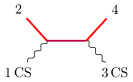
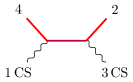
Figure 3: The $s$- and $u$-channel exchanges of excitations mediating a Compoton-like scattering of CSPs.

Contrary to the previous examples, this result is uniquely fixed by matching an ansatz to its factorisation channels. For instance, any deformation of the denominators in the exponentials, e.g.

$$\frac{1}{s-m^{2}}\to\frac{1}{(1+\alpha)s-m^{2}-\alpha m^{\prime 2}}\ ,$$ (4.14)

and likewise for the $u$-channel, returns identical residues on the factorisation channels, but it would not be compatible with the general covariant properties under LG transformations, fixed in equation (3.27). The latter crucially demands the denominator to be $\langle 1|p_{2}|1]=\langle 3|p_{1}|3]=s-m^{2}$ and analogously for the $u-$channel.

4.4 The partial-wave decomposition of CSPs

In this section, we present the PW decomposition of four (identical) CSPs scattering, following the strategy of reference [25, 27]. We decompose the Poincaré-reducible 2-CSP state into a sum of irreps of definite angular momentum $j$ at the mass $s=m^{2}=2p_{1}\cdot p_{2}=2p_{3}\cdot p_{4}$. That is, we glue two effective three-point amplitudes (3.19) studied in Section 3.2:

$$\mathcal{M}(1^{\theta_{1}}2^{\theta_{2}}\to 3^{\theta_{3}}4^{\theta_{4}})= 16\pi\sum_{\{h_{i}\}}e^{-i(h_{1}\theta_{1}+\ldots+h_{4}\theta_{4})}(-1)^{h_{3}+h_{4}}e^{-i(h_{12}-h_{34})\phi}\times$$ (4.15)

$$\times\sum_{j\geq|h_{12}|\ ,\,|h_{34}|}(2j+1)d^{j}_{h_{12}\,h_{34}}(\theta)\mathcal{M}^{j}_{h_{1}\ldots h_{4}}(s)\times e^{2i\mu\frac{\epsilon_{1}\cdot p_{2}+\epsilon_{2}\cdot p_{1}}{s}}e^{-2i\mu\frac{\epsilon_{3}\cdot p_{4}+\epsilon_{4}\cdot p_{3}}{s}}\ ,$$

where $d^{j}_{h\,h^{\prime}}(\theta)$ are Wigner $d$-matrices, $\theta$ the scattering angle, $\phi$ the rotation of the scattering plane, $h_{ij}\equiv h_{i}-h_{j}$, and $\mathcal{M}^{j}_{h_{1}\ldots h_{4}}$ the ordinary $j$-wave amplitude among massless particles of helicity $h_{i}$. The $(-1)^{h_{3}+h_{4}}$-factor results from crossing particles 3 and 4 to the out-going state, corresponding to work with all-ingoing three-point amplitudes of previous sections and send $\theta_{3,4}\to\theta_{3,4}+\pi$, which also flips the sign of one of the little-group exponentials.

The PW decomposition (4.15) can be inverted to extract the partial waves. This is done by striping off from the amplitude the little-group exponential factors that appear in (4.15), then Fourier transforming the $\theta_{i}$, and at this point project with Wigner-$d$ matrices, as in the familiar case, thanks to their orthogonality.

In the particular example of identical external CSPs (e.g. equation (1)), inverting the PW decomposition partially cancels the LG exponentials on both sides of (4.15). The leftover LG exponential factors on the left-hand side of (4.15) are associated with the $t$ and $u$ channels, while the PW is an expansion in s-channel intermediate states.

4.5 Analytic structure and unitarity

The examples that we have explored allow us to infer some general lessons about the structure of four-point amplitudes involving CSPs.

First, by construction, the pole structure is consistent with (extended) unitarity because we used well-defined three-point amplitudes that respect LG scaling and the mass-splitting selection rule. The amplitudes are also crossing-symmetric and satisfy hermitian analyticity.

Second, the presence of CSPs among initial or final states introduces essential singularities in the Mandelstam variables. Crucially, the latter appear only outside or at the border of the physical region. Their significance w.r.t. extended unitarity deserves further investigation, in connection to the they enter the PW expansion (see Section 4.4).

Third, the exchange of an intermediate — off-shell — CSP is connected to the presence of Bessel functions, although the result is less universal as a family of solutions exists. In particular, tree-level factorisation is not enough to uniquely fix the argument of the Bessel and, due to the intrinsic non-polynomial structure, EFT arguments can not be invoked.

We notice the possibility of a choice without additional singularities in the Mandelstam variables ($\alpha=0$ in equation (4.10)), but singular in the equal-mass limit. In this case the mass-splitting acts as a regulator that cannot be removed. Conversely, the choice $\alpha\neq 0$ introduces essential singularities in the Mandelstam variables at generic values in the complex plane. This seems to violate either (extended) unitarity if the singularity falls on the real axis. Instead, when the singularities appear at imaginary values we should probably observe a violation of causality.

5 Weakening the Assumptions

We have seen in previous sections that requiring factorisation in well-defined on-shell three-point amplitudes is heavily constraining, allowing only a limited set of interactions. For instance, taken at face value, the mass-splitting selection rule together with exact factorisation, would forbid Compton-like scattering among matter particles of the same mass and CSPs. In this section, we therefore explore whether it is possible — and what consequences carries— weakening some of the assumptions.

We consider the possibility of starting directly from the four-point amplitudes, according to the general structure given by (3.27). Notice that, without the input of factorisation, there are not enough constraints to bootstrap the amplitudes, since the four-point kinematics is less stringent. In particular, there are several allowed and inequivalent choices of the vectors $p^{\pm}_{j}$ appearing in the exponential LG prefactors, even though different choices correspond to assigning a different overall (kinematically-dependent) phase to the amplitude. In the following, we explore — with a critical eye but an open mind — some possible strategies to fix these amplitudes.

5.1 Massless and degenerate limits

A first possibility is to consider amplitudes that can be built up using factorisation and then take the massless or equal-mass limit. We explore this possibility in instructive examples.

5.1.1 Compton-like scattering

We consider the process described by the amplitude in equation (4.13). Taking now the equal-mass limit $\Delta m^{2}\to 0$ we get

$$\mathcal{M}(1^{\theta_{1}}2\,3^{\theta_{3}}4)=-e^{i\mu\frac{\epsilon_{1}\cdot p_{2}+\epsilon_{3}\cdot p_{4}}{s-m^{2}}}\frac{\Lambda^{2}}{s-m^{2}}-e^{i\mu\frac{\epsilon_{1}\cdot p_{4}+\epsilon_{3}\cdot p_{2}}{u-m^{2}}}\frac{\Lambda^{2}}{u-m^{2}}$$ (5.1)

This amplitude describes a Compton-like scattering of a mostly-scalar CSP and a massless scalar.

Notice that the essential singularities coming from the exponentials, which before appeared outside the physical region, now overlap with the simple poles at the boundary of the latter. This reflects the absence of the corresponding equal-mass three-point amplitude. The same situation persists if we further take $m\to 0$.

Figure 4: The $s$- and $u$-channel Compoton-like scattering of CSPs in the equal-mass limit.

5.1.2 What about factorisation?

The previous example highlights a crucial feature of amplitudes with CSPs that cannot be obtained via factorisation in three-point amplitudes: the poles that would be related to an on-shell exchange of single particles overlap with the essential singularities that are imposed by little-group covariance. This is directly correlated to the absence of three-point amplitudes violating the mass-splitting selection rule. Are the resulting amplitudes healthy?

First, we observe that we can always imagine these amplitudes to be actually regulated by an infinitesimal mass difference. This allows us to disentangle the poles dictated by unitarity from the kinematical essential singularities. It forces us, however, to work in a regime where all the other mass scales or momenta are larger than the regulator, preventing us from lowering them to zero. For example, this would be an obstruction in taking an exact soft limit. Another example is when the momenta are integrated over, including a region where they are smaller than the mass splitting, see next section. In some cases, one can take a double scaling limit where the momentum is softer than all other scales except for the IR regulator that controls the violation of the mass-splitting selection rule (see the discussion in Section 5.3).

Another possibility is to just define amplitudes as the result of the equal-mass limits, as a prescription. The absence of exact factorisation may not necessarily be a fatal pathology after all, since factorisation is anyway recovered in an approximate sense in the high-energy limit. Indeed, as discussed in Section 3.4, the kinematical LG exponential factors become negligible in the high-energy limit, and the exchange of an on-shell state can be resolved.

To understand if the presence of essential singularities, dictated by this prescription, is pathological, we consider further examples of amplitudes and extract physical observables.

5.1.3 Mostly-scalar CS potential

We study the potential generated by the internal exchange of a mostly-scalar CSP. To this purpose we consider the class of amplitudes described in equation (4.10), now keeping $m_{1}\neq m_{2}$ to remove the $u$-channel, and look at the $s$-channel process:

$$\mathcal{M}(1\,1^{\prime}\,2\,2^{\prime})=-\frac{\Lambda^{2}}{t}J_{0}\!\left(\frac{2\mu\sqrt{-s}}{\alpha t+\Delta m^{2}}\right)\ ,$$ (5.2)

As we discussed, requiring factorisation is not sufficient to fix the amplitude, hence we will discuss some paradigmatic examples.

First, we can consider the case $\alpha=0$:

$$\mathcal{M}(1\,1^{\prime}\,2\,2^{\prime})=-\frac{\Lambda^{2}}{t}J_{0}\!\left(\frac{2\mu\sqrt{-s}}{\Delta m^{2}}\right)\ ,$$ (5.3)

The amplitude has the analytic structure dictated by unitarity, nevertheless it is singular in the equal-mass limit. Therefore, we will keep $\Delta m^{2}$ as a regulator, that cannot be completely removed, and keep track of it only where necessary. In order to extract the potential induced by this exchange we evaluate the amplitude in the center-of-mass (CoM) kinematics:

$$\begin{split}&p_{1}=(\omega_{1},\vec{p}+\frac{\vec{q}}{2})\ ,\quad p^{\prime}_{1}=(\omega_{1},\vec{p}-\frac{\vec{q}}{2})\ ,\quad p_{2}=(\omega_{2},-\vec{p}-\frac{\vec{q}}{2})\ ,\quad p^{\prime}_{2}=(\omega_{2},-\vec{p}+\frac{\vec{q}}{2})\ ,\end{split}$$ (5.4)

with $\vec{p}\cdot\vec{q}=0$, $\omega_{1,2}^{2}=p^{2}+\frac{q^{2}}{4}+m_{1,2}^{2}$, $s=(\omega_{1}+\omega_{2})^{2}$ and $t=-\vec{q}^{2}$. In the static limit $s\sim(m_{1}+m_{2})^{2}$, we find

$$\mathcal{M}(1\,1^{\prime}\,2\,2^{\prime})\simeq\frac{\Lambda^{2}}{q^{2}}I_{0}\!\left(\frac{2\mu(m_{1}+m_{2})}{\Delta m^{2}}\right)\ ,$$ (5.5)

where $I_{0}$ is the modified Bessel function of the first kind. The potential is obtained from a three-dimensional Fourier transform:

$$V(\vec{x})=\frac{-1}{4m_{1}m_{2}}\int\frac{d^{3}q}{(2\pi)^{3}}e^{i\vec{q}\cdot\vec{x}}\mathcal{M}(1\,1^{\prime}\,2\,2^{\prime})\ .$$ (5.6)

The $\vec{q}$ integral is then trivial and yields:

$$V(\vec{x})=-\frac{\Lambda^{2}}{16\pi m_{1}m_{2}}\frac{1}{r}I_{0}\!\left(\frac{2\mu(m_{1}+m_{2})}{\Delta m^{2}}\right)\ ,$$ (5.7)

where $r$ is the radius in the spherical coordinates. The potential has a standard $\frac{1}{r}$ scaling, but a non-trivial dependence on the masses. Even at short distances the scale $\mu$ cannot be neglected and all the helicities are exchanged, unless we take $\Delta m^{2}\gg\mu^{2}$ as well. In this case, only $h=0$ is effectively exchanged.

Then, we consider the case with $\alpha\neq 0$. The analytic structure of this amplitude presents several singular points, as discussed. Moreover, if the regulator is removed at the level of the amplitude sending $\Delta m^{2}\to 0$ we lose manifest factorisation, since the essential singularity overlaps with the simple pole at $t=0$. We just report the results obtained for the potential, keeping a finite mass-splitting until the very end of the computation. A general feature is that at short distance $r\mu\ll 1$ we recover the standard scalar potential:

$$V(\vec{x})\overset{r\mu\ll 1}{\sim}-\frac{\Lambda^{2}}{16\pi m^{2}}\frac{1}{r}\ ,$$ (5.8)

as a consequence of the good UV behaviour. Then we can distinguish two cases:

1. When the singularities are on the real axis (e.g. $\alpha=1$ in equation (5.2)), at intermediate distances $\frac{1}{\mu}\ll r\ll\frac{1}{\Delta m^{2}}$ the potential oscillates around $0$ with exponentially growing amplitude, while for distances $r\gg\frac{1}{\Delta m^{2}}$ the mass-splitting acts as a regulator and the potential tends to equation (5.7). If the regulator is removed, the intermediate regime with exponentially large oscillations extends up to infinite distances.

2. When the singularities are on the imaginary axis, e.g. choosing:

   $$\mathcal{M}(1\,1^{\prime}\,2\,2^{\prime})=-\frac{\Lambda^{2}}{2t}\left[J_{0}\!\left(\frac{2\mu\sqrt{-s}}{it+\Delta m^{2}}\right)+J_{0}\!\left(\frac{2\mu\sqrt{-s}}{-it+\Delta m^{2}}\right)\right]\ ,$$ (5.9)

   at intermediate distances $\frac{1}{\mu}\ll r\ll\frac{1}{\Delta m^{2}}$ the potential oscillates around $0$ with an exponential amplitude decaying as $r^{-\frac{5}{3}}$, while for distances $r\gg\frac{1}{\Delta m^{2}}$ the mass-splitting acts as a regulator and the potential tends to equation (5.7). If the regulator is removed, the intermediate regime with polynomially small oscillations extends up to infinite distance.

Figure 5: The $t$-channel exchange of a CSP in the equal-mass limit.

5.2 How do CS photons gravitate?

In this section, we would like to address the question of whether we can couple CSPs to standard gravity and compute the momentum kick from the gravitational coupling. To this end, we consider the coupling to a massive spin-2 particle, the contribution to the amplitude from its exchange and its massless limit. To single out only the graviton in the massless limit, we will consider mostly-vectors CSPs in the external states.

The relevant three-point amplitudes are

$$\mathcal{M}(1^{\theta_{1}}2^{\theta_{2}}3^{j=2})=\frac{\kappa}{2}e^{i\mu\frac{\epsilon_{1}\cdot p_{2}+\epsilon_{2}\cdot p_{1}}{p_{1}\cdot p_{2}}}\cdot\left[\frac{\langle 1\boldsymbol{3}\rangle^{4}}{\langle 12\rangle^{2}}e^{i(\theta_{1}-\theta_{2})}+\frac{\langle 2\boldsymbol{3}\rangle^{4}}{\langle 12\rangle^{2}}e^{-i(\theta_{1}-\theta_{2})}\right]\ ,$$ (5.10)

and

$$\mathcal{M}(123^{j=2})=\frac{\kappa}{2}\frac{\langle\boldsymbol{3}|p_{1}|\boldsymbol{3}]^{2}}{M^{2}}\ ,$$ (5.11)

where $M$ is the mass of the graviton. The resulting contribution to the four-point amplitude is

$$\mathcal{M}_{4}(1^{\theta_{1}}\phi\,\phi\,4^{\theta_{4}})=-\left(\frac{\kappa}{2}\right)^{2}e^{2i\mu\frac{\epsilon_{1}\cdot p_{4}+\epsilon_{4}\cdot p_{1}}{t}}\left[\frac{\langle 1|p_{2}|4]^{2}}{t-M^{2}}e^{i(\theta_{1}-\theta_{4})}+\frac{\langle 4|p_{2}|1]^{2}}{t-M^{2}}e^{i(\theta_{4}-\theta_{1})}\right]\ .$$ (5.12)

We could have obtained the amplitude, with $M=0$, simply by dressing the gravitational amplitude of a photon-scalar scattering with the proper exponential factor. In principle, we may consider this as the defining procedure for mostly-$h$ CSP-scalar amplitudes, for $h\neq 1$. We leave this exploration for future works.

We can now compute the momentum kick to the CSP scattering off the gravitational potential generated by the scalar $\phi$, after taking $M\to 0$. Following the discussion in reference [29]: we consider an initial state which is a superposition of two-particle (the CSP and the scalar) states

$$|\psi\rangle_{\rm in}=\int_{0}^{2\pi}\!\differential\theta\int\!\differential\Phi(p_{1})\differential\Phi(p_{2})\,\Psi(\theta)\Psi(p_{1})\Psi(p_{2})\,e^{i(p_{1}+p_{2})\cdot b}\,|p_{1}\,\theta,p_{2}\rangle\ ,$$ (5.13)

where $\differential\Phi(p_{i})$ is the Lorentz-invariant phase-space measure for the particle $p_{i}$, $\Psi(p_{i})$ and $\Psi(\theta)$ are the wavefunctions describing the momenta of the incoming particles and the helicity distribution of the CSP, respectively. $b^{\mu}$ is the impact parameter between the two incoming wavepackets.

Figure 6: The $t$-channel exchanges of massive graviton.

Then, the momentum kick is given by the difference of the expectation values of the momentum operator in out and in states:

$$\Delta p^{\mu}_{\rm CS}=\,_{\rm in}\langle\psi|S^{\dagger}[P_{1}^{\mu},S]|\psi\rangle_{\rm in}\ .$$ (5.14)

Expanding the $S$-matrix in perturbation theory, at leading order we find

$$\Delta p^{\mu}_{\rm CS}=\left\langle\int\!\frac{\differential^{4}q}{(2\pi)^{2}}\,\delta(2p_{1}\cdot q)\delta(2p_{2}\cdot q)e^{ib\cdot q}\,iq^{\mu}\left.\mathcal{M}_{4}(\text{CS}^{h=-1}\phi\,\phi\,\text{CS}^{h=+1})\right|_{\begin{subarray}{c}p_{3}=-p_{2}-q\\ p_{4}=-p_{1}+q\end{subarray}}+\dots\right\rangle\ ,$$ (5.15)

where the dots stand for radiative contributions, $q$ measures the momentum mismatches of the two wavepackets [29] and $\langle\cdot\rangle$ is a short-hand notation for the integration of the result against the chosen wavepackets in $\theta$. Indeed, since we are interested in the large-impact-parameter limit, the wavepackets $\Psi(p_{1})$ have been chosen such that the characteristic lengths of the particles are much smaller than the impact parameter. This is equivalent to taking the limit of large orbital angular momentum, i.e. the eikonal limit. This will keep only the leading terms in the small-$t$ expansion. Thus, the four-point amplitude must be truncated to the leading order in $t=q^{2}$. It is advantageous to rewrite the Fourier integrals using the parametrisation introduced in reference [30]:

$$q^{\mu}=z_{1}\,\frac{p_{1}^{\mu}}{\sqrt{s-m^{2}}}+z_{2}\,\frac{p_{2}^{\mu}}{\sqrt{s-m^{2}}}+z_{b}\frac{b^{\mu}}{\sqrt{-b^{2}}}+z_{v}\frac{v^{\mu}}{\sqrt{-v^{2}}}\ ,$$ (5.16)

where $v^{\mu}=\epsilon^{\mu\nu\rho\sigma}p_{1\nu}p_{2\rho}b_{\sigma}$, the $z$’s are the new integration variables and $m$ is the mass of the scalar $\phi$. The delta functions fix $z_{1}=0$ and $z_{2}=0$. The spinors can be rewritten in terms of Mandelstams:

$$\begin{split}\langle 1|p_{2}|4]^{2}&=-e^{-i\Delta\phi}\left[(s-m^{2})^{2}+st\right]=-(s-m^{2})^{2}+\mathcal{O}(q^{2})\ ,\\ \langle 4|p_{2}|1]^{2}&=-e^{+i\Delta\phi}\left[(s-m^{2})^{2}+st\right]=-(s-m^{2})^{2}+\mathcal{O}(q^{2})\ .\end{split}$$ (5.17)

Thus, we find

$$\begin{split}\Delta p^{\mu}_{\rm CS}=\left\langle-\frac{i\,\kappa^{2}}{(4\pi)^{2}}\int\!\differential^{2}z\,e^{-i\sqrt{-b^{2}}z_{b}}e^{-2i\mu\frac{z_{b}\frac{(\epsilon_{1}+\epsilon_{4})\cdot b}{\sqrt{-b^{2}}}+z_{v}\frac{(\epsilon_{1}+\epsilon_{4})\cdot v}{\sqrt{-v^{2}}}}{z_{v}^{2}+z_{b}^{2}}}\left(z_{b}\frac{b^{\mu}}{\sqrt{-b^{2}}}+z_{v}\frac{v^{\mu}}{\sqrt{-v^{2}}}\right)\times\right.\\ \left.\times\frac{(s-m^{2})\cos\delta\theta}{z_{v}^{2}+z_{b}^{2}+M^{2}}\right\rangle\ ,\end{split}$$ (5.18)

where $\delta\theta=\theta_{1}-\theta_{4}$ is a measure of the LG-phase mismatch of the two wavefunctions used to compute the expectation value. We can now introduce polar coordinates on the $\vec{z}$-plane, rescale the radial coordinate with $\sqrt{-b^{2}}$ and integrate over the angle:

$$\begin{split}\Delta p^{\mu}_{\rm CS}=\left\langle\frac{\kappa^{2}\cos\delta\theta}{8\pi\sqrt{-b^{2}}}\int_{0}^{\infty}\!\differential q\,q^{2}\,\frac{|\mathrm{B}_{q}|\frac{b^{\mu}}{\sqrt{-b^{2}}}+\mathrm{V}\frac{v^{\mu}}{\sqrt{-v^{2}}}}{\sqrt{\mathrm{B}_{q}^{2}+\mathrm{V}^{2}}}J_{1}\!\left(\frac{2\sqrt{-b^{2}}\mu}{q}\sqrt{\mathrm{B}_{q}^{2}+\mathrm{V}^{2}}\right)\,\frac{(s-m^{2})}{q^{2}-b^{2}M^{2}}\right\rangle\ ,\end{split}$$ (5.19)

where

$$\mathrm{B}_{q^{2}}=\frac{(\epsilon_{1}+\epsilon_{4})\cdot b}{\sqrt{-b^{2}}}+\frac{q^{2}}{2\sqrt{-b^{2}}\mu}\ ,\quad\text{and}\quad\mathrm{V}=\frac{(\epsilon_{1}+\epsilon_{4})\cdot v}{\sqrt{-v^{2}}}\ .$$ (5.20)

Now we can set $M=0$ and consider two limiting cases:

$$\begin{split}\Delta p^{\mu}_{\rm CS}&\overset{\sqrt{-b^{2}}\mu\ll 1}{\sim}\frac{\kappa^{2}(s-m^{2})}{8\pi}\frac{b^{\mu}}{(-b^{2})}\left\langle\cos\delta\theta\right\rangle\ ,\\ \Delta p^{\mu}_{\rm CS}&\overset{\sqrt{-b^{2}}\mu\gg 1}{\sim}\frac{\kappa^{2}(s-m^{2})}{8\pi}\frac{b^{\mu}}{(-b^{2})}\left\langle\cos\delta\theta\,J_{0}\!\left(2(-b^{2}\mu^{2})^{\frac{1}{4}}\sqrt{\mathrm{B}_{0}+\sqrt{\mathrm{B}_{0}^{2}+\mathrm{V}^{2}}}\right)\right\rangle\ .\end{split}$$ (5.21)

We notice that we recover the usual result from Einstein-Hilbert gravity in the UV, as expected. For intermediate impact parameters $\sqrt{-b^{2}}\mu\sim 1$, the momentum is deflected outside the scattering plane, by spin-orbit-like contributions. At large distances, the scattering happens in the scattering plane (the spin-orbit interactions are averaged away), and the deflection oscillates rapidly and decays as $(\sqrt{-b^{2}}\mu)^{-1/4}$:

$$J_{0}(x)\overset{x\gg 1}{\sim}\sqrt{\frac{2}{\pi}}\frac{\cos\left(\frac{\pi}{4}-x\right)}{\sqrt{x}}\ .$$ (5.22)

It is now interesting to study two limiting cases for the wavepackets for the helicity configuration of the CSP. We choose the wavefunctions in the helicity basis because it makes the physics clearer, and then consider the Fourier transform to the $\theta$ basis. We consider a Gaussian and a single-helicity distribution:

$$\Psi_{\Delta h}(h)=\mathcal{N}_{\Delta h}\,e^{-\frac{(h-\bar{h})^{2}}{\Delta h^{2}}}\ ,\qquad\Psi_{\hat{h}}(h)=\delta_{h\hat{h}}\ ,$$

where $\mathcal{N}_{\Delta h}$ is a proper normalisation such that $\sum_{h=-\infty}^{+\infty}|\Psi(h)|^{2}=1$. In the $\theta$ basis, the wavepackets become

$$\Psi_{\Delta h}(\theta)=\mathcal{N}_{\theta}\,\Delta h\,e^{-\frac{1}{4}\theta^{2}\Delta h^{2}-i\bar{h}\theta}\,\vartheta_{3}\!\left(-\pi\bar{h}+\frac{1}{2}i\pi\Delta h^{2}\theta,e^{-\pi^{2}\Delta h^{2}}\right)\ ,\qquad\Psi_{\hat{h}}(\theta)=\frac{e^{-i\hat{h}\theta}}{2\pi}\ ,$$

where $\vartheta_{3}$ is a Jacobi elliptic theta function. For flat helicities distributions $\Delta h\gg 1$, $\Psi_{\Delta h}(\theta)$ becomes sharply peaked around $\theta\sim 0$, i.e. we can take $\Psi_{\Delta h}(\theta)=\delta(\theta)$.

Computing the expectation value in equation (5.19) with a flat distribution is equivalent to taking $\delta\theta\to 0$. Then the integral simplifies drastically. Indeed, the polarisations are fixed as in footnote 12:

$$\begin{split}\epsilon_{4}=-\left.\epsilon_{1}\right|_{\theta_{1}\to\theta_{1}+\delta\theta}+\mathcal{O}(q^{2})\sim-\epsilon_{1}\ ,\end{split}$$ (5.23)

and the scattering angle recovers the GR result for any value of $\sqrt{-b^{2}}\mu$.

On the other hand, in case we consider the initial state to be building out of a single helicity state $\hat{h}$, we find two qualitatively different results.

1. In the UV, only one helicity state is coupled and we have a non-zero deflection iff $\hat{h}=\pm 1$, as expected. The scattering angle is the same as in GR.

2. In the IR, all the helicity states are coupled and we will have a non-trivial contribution from all of them. The scattering angle is analytically similar to the result in GR, up to a $(\sqrt{-b^{2}}\mu)$-dependent factor, coming from the non-trivial angular integration in the second line of equation (5.21).

5.3 Soft limits

An important property of scattering amplitudes is their behaviour when an external massless particle is given soft momentum. In the following, we study this regime amplitudes obtained via the prescription described in the previous section.

5.3.1 Soft CS radiation

As a first example, we consider the limit of soft CSPs. For this purpose, we consider the following five-point amplitude with three external CSPs and two massive particles of equal mass:

$$\mathcal{M}(1^{\theta_{1}}2\,3^{\theta_{3}}4\,5^{\theta_{5}})=e^{i\mu\frac{\epsilon_{1}\cdot p_{2}}{p_{1}\cdot p_{2}}}e^{i\mu\frac{\epsilon_{3}\cdot(p_{4}+p_{5})}{p_{3}\cdot(p_{4}+p_{5})}}e^{i\mu\frac{\epsilon_{5}\cdot p_{4}}{p_{5}\cdot p_{4}}}\frac{\Lambda^{2}}{(p_{1}+p_{2})^{2}-m^{2}}\frac{\Lambda}{(p_{4}+p_{5})^{2}-m^{2}}+\text{(permutations)}\ .$$ (5.24)

Figure 7: One of the diagrams contributing to the 5-point amplitude.

We consider the amplitude in the soft limit $p_{5}\ll p_{i}$:

$$\mathcal{M}(1^{\theta_{1}}2\,3^{\theta_{3}}4\,5^{\theta_{5}})\sim\left[-e^{i\mu\frac{\epsilon_{1}\cdot p_{2}}{p_{1}\cdot p_{2}}}e^{i\mu\frac{\epsilon_{3}\cdot p_{4}}{p_{3}\cdot p_{5}}}\frac{\Lambda^{2}}{(p_{1}+p_{2})^{2}-m^{2}}\right]\cdot\frac{1}{2p_{4}\cdot p_{5}}\left[-\Lambda e^{i\mu\frac{\epsilon_{5}\cdot p_{4}}{p_{5}\cdot p_{4}}}\right]+\text{(permutations)}\ .$$ (5.25)

The other orderings are analogous and, as usual, the soft insertions on internal lines are negligible. Summing all the leading contributions we get

$$\mathcal{M}(1^{\theta_{1}}2\,3^{\theta_{3}}4\,5^{\theta_{5}})\sim\mathcal{M}(1^{\theta_{1}}2\,3^{\theta_{3}}4)\cdot\sum_{i=2,4}\frac{1}{2p_{i}\cdot p_{5}}S_{i}(5^{\theta_{5}})\ ,$$ (5.26)

where we defined the mostly-scalar CS soft factor:

$$S_{i}(5^{\theta_{5}})=-\Lambda e^{i\mu\frac{\epsilon_{5}\cdot p_{i}}{p_{5}\cdot p_{i}}}\ .$$ (5.27)

Thus, the amplitude satisfies factorisation for soft external CSPs. The soft factor has the correct transformation properties under Lorentz and little group and agrees with the results of [14, 15]. This result is easily generalized to any amplitude (at least tree-level) built via factorisation and using the prescription for the equal-mass limit:

$$\mathcal{M}(1...n-1\,n^{\theta_{n}})\sim\mathcal{M}(1...n-1)\cdot\sum_{i}\frac{1}{2p_{i}\cdot p_{n}}S_{i}(n^{\theta_{n}})\ ,$$ (5.28)

where index $i$ runs over all the external scalar legs of the hard amplitude. Notice that this statement comes with a caveat: if we are implicitly assuming the amplitude to be regulated by an infinitesimal mass, then the factorisation in the soft limit should be understood in an approximate sense, that is in the regime in which the soft momentum is larger than the regulator but much smaller than the other external momenta.

5.3.2 Soft non-CS radiation

We consider now the case of non-CS soft external massless legs, in the presence of external CSPs. In particular, we start from the three-point amplitude for two mostly-scalar CSPs and a massive scalar:

$$\mathcal{M}(1^{\theta_{1}}2^{\theta_{2}}3)=\Lambda e^{i\mu\frac{\epsilon_{1}\cdot p_{2}}{p_{1}\cdot p_{2}}}e^{i\mu\frac{\epsilon_{2}\cdot p_{1}}{p_{2}\cdot p_{1}}}\ .$$ (5.29)

We can build the five-point amplitude via factorisation and then take the massless limit. Taking the limit in which particle $5$ is soft, we find

$$\begin{split}\mathcal{M}(1^{\theta_{1}}2^{\theta_{2}}3^{\theta_{3}}4^{\theta_{4}}5)\sim&\frac{\Lambda^{3}}{(p_{1}+p_{2})^{2}}e^{i\mu\frac{\epsilon_{1}\cdot p_{2}}{p_{1}\cdot p_{2}}}e^{i\mu\frac{\epsilon_{2}\cdot p_{1}}{p_{2}\cdot p_{1}}}e^{i\mu\frac{\epsilon_{3}\cdot p_{4}}{p_{3}\cdot p_{4}}}\cdot\\ &\frac{1}{2p_{4}\cdot p_{5}}\int_{0}^{2\pi}\frac{d\theta^{\prime}_{4}}{2\pi}e^{i\mu\frac{\epsilon^{\prime}_{4}\cdot p_{3}}{p_{4}\cdot p_{3}}}e^{-i\mu\frac{\epsilon^{\prime}_{4}\cdot p_{5}}{p_{4}\cdot p_{5}}\frac{p_{3}\cdot p_{4}}{p_{3}\cdot p_{5}}}e^{i\mu\frac{\epsilon_{4}\cdot p_{5}}{p_{4}\cdot p_{5}}}+(\text{permutations})\ ,\end{split}$$ (5.30)

where we have expressed the Bessel function in its integral form. Including permutations, we get

$$\mathcal{M}(1^{\theta_{1}}2^{\theta_{2}}3^{\theta_{3}}4^{\theta_{4}}5)=\sum_{i=1}^{4}\int_{0}^{2\pi}\frac{d\theta^{\prime}_{i}}{2\pi}\mathcal{M}_{4}(...i^{\theta^{\prime}_{i}}...)\frac{1}{2p_{i}\cdot p_{5}}S_{i}(5)\ ,$$ (5.31)

with

$$S_{i}(5)=-\Lambda e^{-i\mu\frac{\epsilon^{\prime}_{i}\cdot p_{5}}{p_{i}\cdot p_{5}}\frac{q_{i}\cdot p_{i}}{q_{i}\cdot p_{5}}}e^{i\mu\frac{\epsilon_{i}\cdot p_{5}}{p_{i}\cdot p_{5}}}\ ,$$ (5.32)

where $q_{i}$ is the momentum of the CS leg attached to the same vertex as the soft particle. Hence, the soft factor depends conformally on another momentum of the hard amplitude and loses in this sense its key feature of universality.

5.4 Backgrounds and pair-wise helicity

As we have seen in Section 3, the main obstruction to building generic three-point amplitudes is the mass-splitting selection rule that emerges from the absence of four-vectors $p^{\pm}_{i}$ in (3.27), when we restrict to (complex) on-shell kinematics where the three particles’ momenta are conserved. Nevertheless, a general feature of $p^{\pm}_{i}$ is that they enter always in a scale-invariant combination, see (3.27). This suggests that we may look at the on-shell three-point amplitude in the presence of a non-trivial background.

Indeed, in presence of an external four-vector $\xi^{\mu}$ we could easily write a three-point amplitude by setting $p^{\pm}_{i}=\xi$ for every CS particle:

$$\mathcal{M}_{3}(\xi)=\prod_{i}\exp\left(\frac{\mu_{i}^{+}}{[i\mathmybb{i}]}\frac{\langle i|\xi|\mathmybb{i}]}{\langle i|\xi|i]}+\frac{\mu_{i}^{-}}{\langle i\mathmybb{i}\rangle}\frac{\langle\mathmybb{i}|\xi|i]}{\langle i|\xi|i]}\right)\widetilde{\mathcal{M}}_{3}\ .$$ (5.33)

This background may e.g. be a plane wave of momentum $\xi^{\mu}$. If now we try to remove the background sending $\xi\to 0$ we notice that the amplitude does not have a well-defined limit, in the sense that it conserves a dependence on the spatial direction.This is effectively an ordinary four-point amplitude in the soft $\xi$-limit of the fourth (spin-0) leg.

This “memory” of arbitrarily soft momenta suggests that CSPs are quite sensitive to infrared boundary conditions at infinity. For instance, it would be interesting to study CSPs amplitudes in the presence of extended objects, such as e.g. strings and monopoles, and possibly uncover a non-trivial interplay between CSPs and topological properties of the environment. We leave this investigation to future work.

In connection with this discussion, we may consider the coupling of CSPs to generic multi-particle states with non-vanishing pair-wise helicity [31]. These states can describe e.g. monopole scattering and the amplitudes can be described as well using spinor-helicity variables [32]. It is unclear whether introducing such states can bring non-trivial kinematics to the three-point amplitudes, and this connection deserves a closer study.

5.5 Non-analytic amplitudes

Up to now we considered the amplitude as an analytic function of the (complex) spinors $|i\rangle$, $|\mathmybb{i}\rangle$, $|i],\ldots$. The physical value of the amplitude is then recovered as a boundary value. This property is correlated to the notion of causality. Nevertheless, from the mathematical point of view, we observe that if we allow the amplitude to depend as well on the complex-conjugate spinors $|i\rangle^{*}$, $|\mathmybb{i}\rangle^{*}$, $|i]^{*},\ldots$, we can construct three-point amplitudes consistent with the little-group constraints. In fact we require the weaker condition that the little group scaling is satisfied only under the real section of the complexified Lorentz group. Hence, we impose

$$(\alpha_{-}\mathbb{W}^{+}_{i}+\alpha_{+}\mathbb{W}^{-}_{i})\mathcal{M}_{\theta_{1}\ldots\theta_{n}}=(\alpha_{-}\mu_{i}^{+}+\alpha_{+}\mu_{i}^{-})\mathcal{M}_{\theta_{1}\ldots\theta_{n}}\ ,$$ (5.34)

for generic complex $\alpha_{-}=(\alpha_{+})^{*}$. Indeed, in the presence of complex-conjugate spinors the representation of the complexified Lorentz algebra is no more complex-linear (but only real-linear). To obtain a linear representation we need to restrict to the real Lorentz algebra. In particular, $W_{\mu}^{2}$ must be expressed as $-W_{1}^{2}-W_{2}^{2}$.

We consider the example of a three-point amplitude with two standard massless (1,2) and one CSP (3). In previous sections, we have seen that analytic solutions to the little-group constraints do not exist. So we start by considering kinematics with $[ij]=0$ and look for non-analytic cases. The only non-trivial brackets under $ISO(2)$ translations are then $\langle\mathmybb{3}1\rangle$ and $\langle\mathmybb{3}1\rangle$, but only a linear combination of the two is independent, thanks to the Schouten identity. Then, consider the following ansatz:

$$\mathcal{M}_{\theta_{3}}=\exp\left(\frac{\mu_{3}^{-}}{\langle 3\mathmybb{3}\rangle}\frac{\langle 1\mathmybb{3}\rangle}{\langle 13\rangle}-\frac{\mu_{3}^{+}}{\langle 3\mathmybb{3}\rangle^{*}}\frac{\langle 1\mathmybb{3}\rangle^{*}}{\langle 13\rangle^{*}}\right)\left(\sum_{h_{3}}\mathcal{M}_{h_{3}}e^{-ih_{3}\theta_{3}}\right)\ ,$$ (5.35)

which satisfies equation (5.34) and the helicity constraint. It is manifest why we cannot look at the complexified LG algebra: indeed, the amplitude is still annihilated by $\mathbb{W^{+}}$, while the transformation under $\mathbb{W^{-}}$ is such that the real generators $W_{1}$ and $W_{2}$ have independent real eigenvalues proportional to $\mu\cos\theta$ and $\mu\sin\theta$. Therefore, we see that imposing LG constraints provides us with a prescription to extend the amplitude to complex kinematics, as an alternative to the analytic continuation. This amounts to a different choice of the $i\epsilon$ prescription, corresponding, in our understanding, to the one of [18]. We remark that the non-analyticity is restricted to the exponential factor, hence in the high-energy limit we recover an analytic amplitude.

We can push this example further and try to build a four-point amplitude. In particular, we consider a mostly-scalar CSP with a coupling to massless scalars. We can take the three-point amplitude in the holomorphic and anti-holomorphic kinematics to be

$$\begin{split}\mathcal{M}^{H}(1\,2\,3^{\theta_{3}})&=\Lambda\exp\left(\frac{\mu_{3}^{-}}{\langle 3\mathmybb{3}\rangle}\frac{\langle 1\mathmybb{3}\rangle}{\langle 13\rangle}-\frac{\mu_{3}^{+}}{\langle 3\mathmybb{3}\rangle^{*}}\frac{\langle 1\mathmybb{3}\rangle^{*}}{\langle 13\rangle^{*}}\right)\ ,\\ \mathcal{M}^{AH}(1\,2\,3^{\theta_{3}})&=\Lambda\exp\left(\frac{\mu_{3}^{+}}{[3\mathmybb{3}]}\frac{[1\mathmybb{3}]}{[13]}-\frac{\mu_{3}^{-}}{[3\mathmybb{3}]^{*}}\frac{[1\mathmybb{3}]^{*}}{[13]^{*}}\right)\ ,\end{split}$$ (5.36)

and a natural ansatz for the Compton scattering is

$$\begin{split}\mathcal{M}(1^{\theta_{1}}2\,3^{\theta_{4}}4)=&-\frac{\Lambda^{2}}{s_{12}}\exp\left(\frac{\mu_{1}^{-}}{\langle 1\mathmybb{1}\rangle}\frac{\langle 2\mathmybb{1}\rangle}{\langle 21\rangle}-\frac{\mu_{1}^{+}}{\langle 1\mathmybb{1}\rangle^{*}}\frac{\langle 2\mathmybb{1}\rangle^{*}}{\langle 21\rangle^{*}}\right)\exp\left(\frac{\mu_{3}^{+}}{[3\mathmybb{3}]}\frac{[4\mathmybb{3}]}{[43]}-\frac{\mu_{3}^{-}}{[3\mathmybb{3}]^{*}}\frac{[4\mathmybb{3}]^{*}}{[43]^{*}}\right)+\\ &-\frac{\Lambda^{2}}{s_{12}}\exp\left(\frac{\mu_{1}^{+}}{[1\mathmybb{1}]}\frac{[2\mathmybb{1}]}{[21]}-\frac{\mu_{1}^{-}}{[1\mathmybb{1}]^{*}}\frac{[2\mathmybb{1}]^{*}}{[21]^{*}}\right)\exp\left(\frac{\mu_{3}^{-}}{\langle 3\mathmybb{3}\rangle}\frac{\langle 4\mathmybb{3}\rangle}{\langle 43\rangle}-\frac{\mu_{3}^{+}}{\langle 3\mathmybb{3}\rangle^{*}}\frac{\langle 4\mathmybb{3}\rangle^{*}}{\langle 43\rangle^{*}}\right)+(2\leftrightarrow 4)\ .\end{split}$$ (5.37)

A weak form of factorisation can be checked by looking at the limits:

$$\begin{split}&\lim_{\langle 12\rangle,[34]\to 0}s_{12}\cdot\mathcal{M}(1^{\theta_{1}}2\,3^{\theta_{4}}4)\ ,\\ &\lim_{[12],\langle 34\rangle\to 0}s_{12}\cdot\mathcal{M}(1^{\theta_{1}}2\,3^{\theta_{4}}4)\ ,\end{split}$$ (5.38)

and analogously for $s_{14}$. Taking the first limit we observe that the second line on equation (5.37) would factorize correctly in the product of three-point amplitudes, nevertheless the first line has essential singularities. Taking the second limit the role of the two lines is just reversed. Even if we included only one of the two lines in the amplitude, there would always be a direction in complex kinematics along which the limit is ill-defined.

This example illustrates the difficulty of defining a non-analytic continuation of the scattering amplitude to complex kinematics satisfying even a weak form of factorisation. We leave for future study the investigation of this problem. Furthermore, even when successfully constructing unitary amplitudes, it would be crucial to understand whether they can be consistent with causality, computing an observable such as e.g. the time delay.

6 Discussion and future directions

In this paper, we initiated the study of continuous-spin particles (CSPs) from the perspective of on-shell consistency conditions. Poincaré invariance, little-group covariance, analyticity, and good high-energy behaviour impose stringent constraints, more so than for ordinary massless particles. We found unique solutions for three-point on-shell amplitudes in the space of functions of bi-spinors, reminiscent of the massive ones, whenever the mass-splitting selection rule is obeyed. In essence, CSPs cannot couple (on-shell, under the given assumptions) to any other pair of particles unless those are non-degenerate in mass. This implies, among other things, that 3-CSPs on-shell amplitudes vanish, as do CSP-particle-antiparticle amplitudes and 2-CSPs-1-graviton amplitudes.

We also classified higher on-shell $n$-point amplitudes and showed that they can be uniquely fixed under favourable conditions. In particular, we bootstrapped on-shell four-point amplitudes for CSPs (with or without ordinary particles) via on-shell factorisation—unitarity—whenever the resulting three-point amplitudes exist. We illustrated these findings through several examples, including the case of intermediate off-shell CSPs. In all cases, the UV amplitudes for CSPs match those of ordinary massless $|h|$-only helicity amplitudes. Infinitely many helicities decouple at short distances, making CSPs a new IR deformation of UV theories, with infinitely many seemingly free degrees of freedom that recouple at low energy.

We also explored various strategies to fix four-point amplitudes when the on-shell three-point function does not exist in a strict sense. Specifically, we examined the consequences of approximate on-shell factorisation, where same-mass particle scattering with CSPs is obtained via a limit of nearly degenerate masses.

Some results obtained this way are ambiguous, depending on whether certain integrations are performed before or after the mass-degenerate limit is taken. For instance, the potential generated by a CSP exchange between ordinary particles of finite spin or helicity falls into this category. If the mass-splitting is removed initially, the results are divergent. Likewise, the soft emission of CSPs among same-mass particles is only approximate, with the soft factors from [14, 15] arising for CSPs momenta softer than any other scales except for the mass splitting of the emitting/absorbing particles.

Conversely, this loose sense of on-shell factorisation works for CSPs coupled to a graviton. By giving the graviton a finite mass during intermediate steps and eventually removing it (along with all longitudinal polarizations) at the level of physical observables, we obtain well-defined results, such as the momentum-kick (equivalently, the scattering angle) calculated in Section 5.2. This suggests that matrix elements for the momentum tensor and two CSPs, $\langle T(q)|p_{1}\,\theta_{1};\,p_{2}\,\theta_{2}\rangle$, indeed exist.

How do our results align with the intriguing findings of [18, 24]? One possibility is that the explicit model presented there—a gauge theory coupled with worldline matter—relaxes some of the basic assumptions about S-matrix theory that we have made in this work. This prompted us to investigate further departures from these assumptions in Section 5.5, where we relaxed strict analyticity (recovered whenever the Pauli-Lubanski scale vanishes and in the high-energy limit). This would allow keeping the little-group exponential factors carried by CSPs real even for complex kinematics, as done in [18, 24] to claim unitarity. However, we have not yet reconciled non-analyticity with on-shell factorisation within the framework of on-shell scattering amplitudes pursued in this manuscript. We believe this important point warrants further analysis, which we leave for future investigations.

Finally, we highlight a couple of directions for further study. While we focused on some consistency conditions, an entire class of stress tests remains, i.e. loop corrections. Are cross-sections for CSPs finite or IR divergent? Do we need to discuss inclusive observables rather than exclusive scattering amplitudes?

Another interesting direction, briefly touched upon in Section 5.4, involves the IR sensitivity of CSPs. Studying CSP theory in the environment of extended objects, such as topological defects, could be insightful.

An obvious question is whether one can construct recursive relations, similar to BCFW, to efficiently reconstruct high $n$-point amplitudes from lower ones. This is a non-trivial task due to the essential singularity appearing in the LG factors of CSPs.

Besides these formal investigations, it would be phenomenologically interesting to calculate how many effective thermalized degrees of freedom $g_{*}(T)$ contribute to the entropy density of our universe at any given temperature, given stringent experimental constraints. Although we have firmly established that scattering amplitudes for CSPs make sense, experiments may have already strongly constrained them.

Acknowledgments

We thank Alfredo Glioti and Pablo Sesma for discussions and early participation. We thank Donal O’Connell for the interesting discussions. SDA is supported by the European Research Council, under grant ERC–AdG–88541.

References

- [1] S. Weinberg, “Infrared Photons and Gravitons,” Phys. Rev. 140 (1965) B516–B524.
- [2] S. Weinberg, “Photons and Gravitons in -Matrix Theory: Derivation of Charge Conservation and Equality of Gravitational and Inertial Mass,” Phys. Rev. 135 (1964) B1049–B1056.
- [3] M. T. Grisaru and H. N. Pendleton, “Soft Spin 3/2 Fermions Require Gravity and Supersymmetry,” Phys. Lett. B 67 (1977) 323–326.
- [4] M. Porrati, “Universal Limits on Massless High-Spin Particles,” Phys. Rev. D 78 (2008) 065016, 0804.4672.
- [5] S. Weinberg and E. Witten, “Limits on Massless Particles,” Phys. Lett. B 96 (1980) 59–62.
- [6] B. Bellazzini, G. Isabella, S. Ricossa, and F. Riva, “Massive gravity is not positive,” Phys. Rev. D 109 (2024), no. 2 024051, 2304.02550.
- [7] B. Bellazzini, F. Riva, J. Serra, and F. Sgarlata, “Massive Higher Spins: Effective Theory and Consistency,” JHEP 10 (2019) 189, 1903.08664.
- [8] F. Bertucci, J. Henriksson, B. McPeak, S. Ricossa, F. Riva, and A. Vichi, “Positivity Bounds on Massive Vectors,” 2402.13327.
- [9] J. Davighi, S. Melville, and T. You, “Natural selection rules: new positivity bounds for massive spinning particles,” JHEP 02 (2022) 167, 2108.06334.
- [10] E. P. Wigner, “On Unitary Representations of the Inhomogeneous Lorentz Group,” Annals Math. 40 (1939) 149–204.
- [11] J. Yngvason, “Zero-Mass Infinite Spin Representations of the Poincare Group and Quantum Field Theory,” Commun. Math. Phys. 18 (1970) 195–203.
- [12] G. J. Iverson and G. Mack, “Quantum Fields and Interactions of Massless Particles - the Continuous Spin Case,” Annals Phys. 64 (1971) 211–253.
- [13] L. F. Abbott and H. J. Schnitzer, “Semiclassical Bound State Methods in Four-Dimensional Field Theory: Trace Identities, Mode Sums, and Renormalization for Scalar Theories,” Phys. Rev. D 14 (1976) 1977.
- [14] P. Schuster and N. Toro, “On the Theory of Continuous-Spin Particles: Wavefunctions and Soft-Factor Scattering Amplitudes,” JHEP 09 (2013) 104, 1302.1198.
- [15] P. Schuster and N. Toro, “On the Theory of Continuous-Spin Particles: Helicity Correspondence in Radiation and Forces,” JHEP 09 (2013) 105, 1302.1577.
- [16] P. Schuster and N. Toro, “A Gauge Field Theory of Continuous-Spin Particles,” JHEP 10 (2013) 061, 1302.3225.
- [17] P. Schuster and N. Toro, “Continuous-Spin Particle Field Theory with Helicity Correspondence,” Phys. Rev. D 91 (2015) 025023, 1404.0675.
- [18] P. Schuster and N. Toro, “Quantum Electrodynamics Mediated by a Photon with Continuous Spin,” Phys. Rev. D 109 (2024), no. 9 096008, 2308.16218.
- [19] V. O. Rivelles, “Gauge Theory Formulations for Continuous and Higher Spin Fields,” Phys. Rev. D 91 (2015), no. 12 125035, 1408.3576.
- [20] V. O. Rivelles, “Remarks on a Gauge Theory for Continuous Spin Particles,” Eur. Phys. J. C 77 (2017), no. 7 433, 1607.01316.
- [21] R. R. Metsaev, “Continuous spin gauge field in (A)dS space,” Phys. Lett. B 767 (2017) 458–464, 1610.00657.
- [22] R. R. Metsaev, “Cubic interaction vertices for continuous-spin fields and arbitrary spin massive fields,” JHEP 11 (2017) 197, 1709.08596.
- [23] I. L. Buchbinder, S. Fedoruk, A. P. Isaev, and A. Rusnak, “Model of Massless Relativistic Particle with Continuous Spin and Its Twistorial Description,” JHEP 07 (2018) 031, 1805.09706.
- [24] P. Schuster, N. Toro, and K. Zhou, “Interactions of Particles with “Continuous Spin” Fields,” JHEP 04 (2023) 010, 2303.04816.
- [25] N. Arkani-Hamed, T.-C. Huang, and Y.-t. Huang, “Scattering Amplitudes for All Masses and Spins,” 1709.04891.
- [26] M. Jacob and G. C. Wick, “On the General Theory of Collisions for Particles with Spin,” Annals Phys. 7 (1959) 404–428.
- [27] M. Jiang, J. Shu, M.-L. Xiao, and Y.-H. Zheng, “Partial Wave Amplitude Basis and Selection Rules in Effective Field Theories,” Phys. Rev. Lett. 126 (2021), no. 1 011601, 2001.04481.
- [28] J. Shu, M.-L. Xiao, and Y.-H. Zheng, “Constructing the general partial wave and renormalization in effective field theory,” Phys. Rev. D 107 (2023), no. 9 095040, 2111.08019.
- [29] D. A. Kosower, B. Maybee, and D. O’Connell, “Amplitudes, Observables, and Classical Scattering,” JHEP 02 (2019) 137, 1811.10950.
- [30] A. Cristofoli, R. Gonzo, D. A. Kosower, and D. O’Connell, “Waveforms from amplitudes,” Phys. Rev. D 106 (2022), no. 5 056007, 2107.10193.
- [31] C. Csáki, S. Hong, Y. Shirman, O. Telem, and J. Terning, “Completing Multiparticle Representations of the Poincaré Group,” Phys. Rev. Lett. 127 (2021), no. 4 041601, 2010.13794.
- [32] C. Csaki, S. Hong, Y. Shirman, O. Telem, J. Terning, and M. Waterbury, “Scattering amplitudes for monopoles: pairwise little group and pairwise helicity,” JHEP 08 (2021) 029, 2009.14213.