Recurrent Stochastic Configuration Networks for Temporal Data Analytics

Abstract

Temporal data modelling techniques with neural networks are useful in many domain applications, including time-series forecasting and control engineering. This paper aims at developing a recurrent version of stochastic configuration networks (RSCNs) for problem solving, where we have no underlying assumption on the dynamic orders of the input variables. Given a collection of historical data, we first build an initial RSCN model in the light of a supervisory mechanism, followed by an online update of the output weights by using a projection algorithm. Some theoretical results are established, including the echo state property, the universal approximation property of RSCNs for both the offline and online learnings, and the convergence of the output weights. The proposed RSCN model is remarkably distinguished from the well-known echo state networks (ESNs) in terms of the way of assigning the input random weight matrix and a special structure of the random feedback matrix. A comprehensive comparison study among the long short-term memory (LSTM) network, the original ESN, and several state-of-the-art ESN methods such as the simple cycle reservoir (SCR), the polynomial ESN (PESN), the leaky-integrator ESN (LIESN) and RSCN is carried out. Numerical results clearly indicate that the proposed RSCN performs favourably over all of the datasets.

Keywords Recurrent stochastic configuration networks, echo state property, universal approximation property, temporal data analytics, nonlinear system modelling.

1 Introduction

Modelling complex dynamics is crucial for industrial process control. Neural networks (NNs) possess the ability to capture intricate nonlinear relationships within dynamic systems, making them effective for problem-solving [1, 2]. As a class of data-driven techniques, the model performance of NNs is significantly influenced by input variables. In real industrial processes, however, system inputs are typically multivariable, with each variable exhibiting a certain delay. The impact of the current input on the system may not be immediately apparent and can evolve over time. These time-varying delays resulting from changes in the controlled plant and external disturbances may lead to systems with unknown or uncertain dynamic orders, posing challenges to both modelling and control tasks [3, 4]. Therefore, developing advanced NN-based strategies is crucial for modelling nonlinear systems with order uncertainty.

Early in [5, 6], variable selection methods had been applied to identify the system order. Among them, multivariate statistical analysis examined the relationships between variables to synthesize their statistical patterns, with principal component analysis (PCA) and partial least squares (PLS) emerging as the most used algorithms for identifying important input information. Moreover, scholars have presented various techniques, such as Bayesian methods, piecewise linearization, conditional probability and mutual information analysis, to extract significant order variables [7, 8, 9]. Unfortunately, identifying the relevant variables can be intricate and time-consuming, and these approaches cannot guarantee real-time tracking within the sampling period. On the other hand, the valuable order and delay information is often embedded in the historical data. In [10], the autoregressive moving average (ARMA) model was proposed to predict the output sequence utilizing historical information. Subsequently, a nonlinear autoregressive moving average (NARMAX) framework incorporating exogenous inputs was introduced for nonlinear dynamic processes in [11]. Nonetheless, both approaches rely on stringent assumptions and exhibit subpar performance when faced with data containing intricate long-term dependencies. Recurrent neural networks (RNNs) have feedback connections between neurons, which can handle the uncertainty caused by the selected input variables that are fed into a learner model. However, training RNNs based on the back-propagation algorithm suffers from the drawbacks of learning parameter setting, slow convergence, and local minima. With such a background, randomized methods for training RNNs have received considerable attention and some extensions have been reported, for instance, echo state networks (ESNs) [12] and liquid state machines [13]. Unfortunately, these methods lack a basic understanding on both the structure design and the random parameters assignment [14]. Our findings reported in [15, 16] motivate us to further investigate modelling complex dynamics using an advanced randomized learner model, termed stochastic configuration networks (SCNs), which are constructed incrementally by assigning the random parameters in the light of a supervisory mechanism.

This paper presents a recurrent version of SCNs (RSCNs) for modelling nonlinear systems with uncertain dynamic orders. The RSCN can be regarded as an incrementally built ESN that inherits the echo state property (ESP) while focusing on addressing the issues of parameter selection and structure setting. Given a collection of historical data, the initial model is trained using the recurrent stochastic configuration (RSC) algorithm. Then, the output weights are dynamically adjusted according to the real-time data. This hybrid learning scheme guarantees the network’s universal approximation performance for both the offline and online learnings, and the detailed theoretical proofs are provided in this paper. Experimental results demonstrate that RSCNs outperform other classical models in terms of learning and generalization performance, indicating their effectiveness in handling nonlinear complex dynamics. Thus, the proposed approach has the following advantages.

• RSCNs operate with partial orders derived from the prior knowledge, eliminating the necessity for explicit order identification. By leveraging the historical process information, RSCNs can accurately predict current outputs, highlighting their ability to capture temporal dependencies and dynamics.

• RSCNs utilize an adaptive and data-dependent parameter scope and construct a special structure of the random feedback matrix in the light of a supervisory mechanism, which allows them to hold the universal approximation property and echo state property, resulting in superior nonlinear processing and temporal data analysis capability.

• An online update of output weights is carried out by using the projection algorithm. This online learning process enables the model to rapidly adjust to dynamic system changes and ensures the convergence of learning parameters, which is crucial for improving the model’s adaptability and maintaining its stability.

The arrangement of this paper is as follows. Section 2 presents the problem formulation and reviews related knowledge of ESNs and SCNs. Section 3 details RSCNs and provides some theoretical analysis. Section 4 reports our experiment results with several comparisons. Finally, Section 5 concludes this paper.

2 Related work

2.1 Problem formulation

Consider a discrete unknown nonlinear system

$$\begin{array}[]{l}y\left({n+1}\right)={f_{\rm{p}}}\left({y\left(n\right),\ldots,y\left({n-{d_{A}}+1}\right),u\left(n\right),}\right.\left.{\ldots,u\left({n-{d_{B}}+1}\right)}\right)+e\left(n\right),\end{array}$$ (1)

where $y,u,e$ are the plant output, control input and process error, respectively, ${{d}_{A}},{{d}_{B}}$ are the systems orders for $y$ and $u$, ${{f}_{\text{p}}}$ is a nonlinear function. Due to external disturbances and changes in the process environment, time-varying delays and unknown orders may occur in the system, leading to poor model performance. However, order identification will inevitably increase computational complexity. This paper aims to tackle the challenges of modelling nonlinear systems with uncertain dynamic orders. By collecting the historical order information, the previous plant output and control input are used to calculate the current output, that is, $y\left(n+1\right)={{f}_{\text{p}}}\left(y\left(n\right),u\left(n\right)\right)+e\left(n\right)$.

2.2 Echo state networks

ESNs exploit the reservoir to map the input signal to a high-dimensional and intricate state space. Unlike RNNs, ESNs randomly assign the input weights and biases, with output weights determined using the least squares method instead of iterative optimization. This helps to avoid the drawbacks of slow convergence and easily falling into local minima. Moreover, ESNs have the echo state property [12], where the reservoir state $\mathbf{x}\left(n\right)$ is the echo of the input and $\mathbf{x}\left(n\right)$ should asymptotically depend on the driving input signal. Recent research on ESNs has focused on investigating the dynamic properties of the reservoir [17, 18], optimizing reservoir parameters [19, 20], and designing reservoir topology [21, 22, 23].

Consider an ESN model with $N$ reservoir nodes

$${\bf{x}}(n)=g({{\bf{W}}_{{\rm{in,}}N}}{\bf{u}}(n)+{{\bf{W}}_{{\mathop{\rm r}\nolimits}{\rm{,}}N}}{\bf{x}}(n-1)+{{\bf{b}}_{N}}),$$ (2)

$${\bf{y}}(n)={{\bf{W}}_{{\mathop{\rm out}\nolimits}{\rm{,}}N}}\left({{\bf{x}}(n),{\bf{u}}(n)}\right),$$ (3)

where $\mathbf{u}(n)\in{{\mathbb{R}}^{K}}$ is the input signal, $\mathbf{x}(n)\in{{\mathbb{R}}^{N}}$ is the internal state vector of the reservoir, ${{\mathbf{b}}_{N}}$ is the bias, ${{\bf{W}}_{{\mathop{\rm out}\nolimits}{\rm{,}}N}}\in{{\mathbb{R}}^{L\times\left(N+K\right)}}$ is the output weight matrix, $K$ and $L$ are the dimensions of input and output, respectively, and $g\left(x\right)$ is the activation function. The input weight matrix ${{\mathbf{W}}_{\operatorname{in},N}}$ and feedback matrix ${{\bf{W}}_{{\mathop{\rm r}\nolimits}{\rm{,}}N}}$ can be defined as follows

$$\begin{array}[]{l}{{\bf{W}}_{{\mathop{\rm in}\nolimits},N}}=\left[{\begin{array}[]{*{20}{c}}{w_{{\mathop{\rm in}\nolimits}}^{1,1}}&{w_{{\mathop{\rm in}\nolimits}}^{1,2}}&\cdots&{w_{{\mathop{\rm in}\nolimits}}^{1,K}}\\ {w_{{\mathop{\rm in}\nolimits}}^{2,1}}&{w_{{\mathop{\rm in}\nolimits}}^{2,2}}&\cdots&{w_{{\mathop{\rm in}\nolimits}}^{2,K}}\\ \vdots&\vdots&\vdots&\vdots\\ {w_{{\mathop{\rm in}\nolimits}}^{N,1}}&{w_{{\mathop{\rm in}\nolimits}}^{N,2}}&\cdots&{w_{{\mathop{\rm in}\nolimits}}^{N,K}}\end{array}}\right]\in{{}^{N\times K}},\\ {\kern 1.0pt}{\kern 1.0pt}{\kern 1.0pt}{{\bf{W}}_{{\mathop{\rm r}\nolimits}{\rm{,}}N}}{\kern 1.0pt}{\kern 1.0pt}{\rm{=}}{\kern 1.0pt}{\kern 1.0pt}{\kern 1.0pt}{\kern 1.0pt}\left[{\begin{array}[]{*{20}{c}}{w_{\mathop{\rm r}\nolimits}^{1,1}}&{w_{\mathop{\rm r}\nolimits}^{1,2}}&\cdots&{w_{\mathop{\rm r}\nolimits}^{1,N}}\\ {w_{\mathop{\rm r}\nolimits}^{2,1}}&{w_{\mathop{\rm r}\nolimits}^{2,2}}&\cdots&{w_{\mathop{\rm r}\nolimits}^{2,N}}\\ \vdots&\vdots&\vdots&\vdots\\ {w_{\mathop{\rm r}\nolimits}^{N,1}}&{w_{\mathop{\rm r}\nolimits}^{N,2}}&\cdots&{w_{\mathop{\rm r}\nolimits}^{N,N}}\end{array}}\right]\in{{}^{N\times N}}.\end{array}$$ (4)

$w_{\operatorname{in}}^{i,j}$ and $w_{\operatorname{r}}^{i,j}$ are generated from a uniform distribution over $\left[-\lambda,\lambda\right]$, and they remain fixed once initialized. Define $\mathbf{X}\text{=}\left[\left(\mathbf{x}(1),\mathbf{u}(1)\right),\ldots,\left(\mathbf{x}({{n}_{\max}}),\mathbf{u}({{n}_{\max}})\right)\right]$, where ${{n}_{\max}}$ is the number of samples, the model output is

$${\bf{Y}}=\left[{{\bf{y}}\left(1\right),{\bf{y}}\left(2\right),...,{\bf{y}}\left({{n_{max}}}\right)}\right]={\bf{W}}_{{\mathop{\rm out}\nolimits},N}{\bf{X}}.$$ (5)

The output weight matrix ${{\mathbf{W}}_{\rm out}}$ can be obtained by the least square method

$$\mathop{\min}\limits_{{\bf{W}}_{{\mathop{\rm out}\nolimits},N}}\left\|{{\bf{W}}_{{\mathop{\rm out}\nolimits},N}{\bf{X}}-{\bf{T}}}\right\|^{2},$$ (6)

$${\bf{W}}_{{\mathop{\rm out}\nolimits},N}^{\top}={\left({{\bf{X}}{{\bf{X}}^{\top}}}\right)^{-1}}{\bf{X}}{{\bf{T}}^{\top}},$$ (7)

where $\mathbf{T}=\left[\mathbf{t}\left(1\right),\mathbf{t}\left(2\right),...,\mathbf{t}\left({{n}_{max}}\right)\right]$ is the desired output signal. In the training process, the initial reservoir state $\mathbf{x}\left(0\right)$ is initialized as a zero matrix and a few warm-up samples are washed out to minimize the impact of the initial zero states.

Remark 1

The scaling factor $\lambda$ is important for adjusting the input data to an appropriate range and converting them to a reasonable interval for the activation function. Original ESNs set a fixed $\lambda$ without constraints on its size, leading to ill-posedness. To address this issue, scholars have suggested various optimization strategies [19, 21, 24]. However, the optimization process will add complexity to the algorithm, creating a trade-off between achieving higher prediction accuracy and maintaining computational efficiency. Therefore, it is crucial to choose a data-dependent and adjustable $\lambda$.

2.3 Stochastic configuration networks

As a class of randomized learner models, SCNs innovatively introduce a supervisory mechanism to assign random parameters in an adaptive interval, ensuring the universal approximation property of the network. SCN construction can be easily implemented, and the resulting model has sound performance for both learning and generalization, which are important to complex dynamic modelling [25, 26, 27]. For more details about SCNs, readers can refer to [16].

Given the objective function $f$, assume that a single-layer feedforward network with $N-1$ hidden layer nodes has been constructed,

$${f_{N-1}}=\sum\limits_{j=1}^{N-1}{{{\bf{\beta}}_{j}}{g_{j}}\left({{\bf{w}}_{j}^{\top}{\bf{u}}+{{\bf{b}}_{j}}}\right)}\left({{f_{0}}=0,N=1,2,3...}\right),$$ (8)

where ${{\mathbf{\beta}}_{j}}={{\left[{{\beta}_{j,1}},{{\beta}_{j,2}},...{{\beta}_{j,L}}\right]}^{\top}}$ is the output weight of the $j$th hidden layer node, $L$ is the number of output layer nodes, ${{g}_{j}}$ is the activation function, ${{\mathbf{w}}_{j}}$ and ${{\mathbf{b}}_{j}}$ are the input weight and bias, respectively. The residual error between the current model output ${{f}_{N-1}}$ and the expected output ${{f}_{\text{exp}}}$ is expressed as

$${e_{N-1}}={f_{{\rm{exp}}}}-{f_{N-1}}=\left[{{e_{N-1,1}},{e_{N-1,2}},...{e_{N-1,L}}}\right].$$ (9)

If ${{\left\|{{e}_{N-1}}\right\|}_{F}}$ does not reach a pre-defined tolerance level, it is necessary to generate a new random basis function ${{g}_{N}}$ under the supervisory mechanism, where ${{\left\|\bullet\right\|}_{F}}$ represents the F norm. The incremental construction process of SCNs can be summarized as follows.

Step 1: Initialize the parameter scalars $\mathbf{\gamma}\text{=}\left\{{{\lambda}_{\min}}:\Delta\lambda:{{\lambda}_{\max}}\right\}$, error tolerance $\varepsilon$, the maximum number of stochastic configurations ${{G}_{\max}}$, the maximum hidden layer size ${{N}_{\max}}$, and residual error ${{e}_{0}}={{e}_{N-1}}$.

Step 2: Assign ${{\mathbf{w}}_{N}}$ and ${{\mathbf{b}}_{N}}$ stochastically in ${{G}_{\max}}$ times from the adjustable uniform distribution $\left[-{{\lambda}_{i}},{{\lambda}_{i}}\right]$ to obtain the candidates of basis function ${{g}_{N}}\left(\mathbf{w}_{N}^{\top}\mathbf{u}+{{\mathbf{b}}_{N}}\right)$, which needs to satisfy the inequality constraint

$${\left\langle{{e_{N-1,q}},{g_{N}}}\right\rangle^{2}}\geq b_{g}^{2}(1-r-{\mu_{N}})\left\|{{e_{N-1,q}}}\right\|^{2},q=1,2,...L$$ (10)

where ${{\lambda}_{i}}\in\mathbf{\gamma}$, $0<r<1$, and $\left\{{{\mu}_{N}}\right\}$ is a nonnegative real sequence that satisfies $\underset{N\to\infty}{\mathop{\lim}}\,{{\mu}_{N}}=0$ and ${{\mu}_{N}}\leq(1-r)$, $0<\left\|g\right\|<{{b}_{g}}$.

Step 3: A set of variables ${{\xi}_{N}}\text{=}\left[{{\xi}_{N,1}},{{\xi}_{N,2}},...,{{\xi}_{N,L}}\right]$ is given to seek the node making the training error converge as soon as possible

$${\xi_{N,q}}=\frac{{{{\left({e_{N-1,q}^{\top}{g_{N}}}\right)}^{2}}}}{{g_{N}^{\top}{g_{N}}}}-\left({1-{\mu_{N}}-r}\right)e_{N-1,q}^{\top}e_{N-1,q}.$$ (11)

A larger positive value $\xi_{N}\text{=}\sum\limits_{q=1}^{L}{{{\xi}_{N,q}}}$ means that the new node is better configured.

Step 4: Update the output weights based on the global least square method

$$\left[{{\bf{\beta}}_{1}^{*},{\bf{\beta}}_{2}^{*},...,{\bf{\beta}}_{N}^{*}}\right]=\mathop{\arg\min}\limits_{\bf{\beta}}{\left\|{{f_{{\rm{exp}}}}-\sum\limits_{j=1}^{N}{{{\bf{\beta}}_{j}}{g_{j}}}}\right\|^{2}}.$$ (12)

Step 5: Calculate the current residual error ${{e}_{N}}$ and renew ${{e}_{0}}:={{e}_{N}}$. Next, update $N:=N+1$, and repeat Step 2-4 until ${{\left\|{{e}_{0}}\right\|}_{F}}\leq\varepsilon$ or $N\geq{{N}_{\max}}$.

At last, we have $\underset{N\to\infty}{\mathop{\lim}}\,\left\|{{f}_{\text{exp}}}-{{f}_{N}}\right\|=0.$

3 Recurrent stochastic configuration networks

3.1 Algorithm description

Given an RSCN model

$${\bf{x}}(n)=g({{\bf{W}}_{{\rm{in}}}}{\bf{u}}(n)+{{\bf{W}}_{\mathop{\rm r}\nolimits}}{\bf{x}}(n-1){\rm{+}}{\bf{b}}),$$ (13)

$${\bf{y}}(n)={{\bf{W}}_{\rm{out}}}\left({{\bf{x}}(n),{\bf{u}}(n)}\right),$$ (14)

randomly assign the input weight matrix and biases for the first reservoir node, ${{\mathbf{W}}_{\operatorname{in},1}}=\left[\begin{matrix}w_{\operatorname{i}\operatorname{n}}^{1,1}&w_{\operatorname{i}\operatorname{n}}^{1,2}&\cdots&w_{\operatorname{i}\operatorname{n}}^{1,K}\\ \end{matrix}\right],$ ${{\mathbf{W}}_{\text{r},1}}\text{=}w_{\operatorname{r}}^{1,1}$, ${{\mathbf{b}}_{1}}={{b}_{1}},$ $w_{\operatorname{in}}^{1,j},w_{\operatorname{r}}^{1,1},{{b}_{1}}\in\left[-\lambda,\lambda\right]$. Then, we add nodes in the light of a supervisory mechanism. As shown in Figure 1, a special reservoir structure is introduced, where only the weights of the new node to the original nodes and itself are assigned, and the weights of other nodes to the new node are set to zero. The feedback matrix can be rewritten as

$$\begin{array}[]{l}{{\bf{W}}_{\rm{r},2}}{\rm{=}}\left[{\begin{array}[]{*{20}{c}}{w_{\mathop{\rm r}\nolimits}^{1,1}}&0\\ {w_{\mathop{\rm r}\nolimits}^{2,1}}&{w_{\mathop{\rm r}\nolimits}^{2,2}}\end{array}}\right],\\ {{\bf{W}}_{\rm{r},3}}{\rm{=}}\left[{\begin{array}[]{*{20}{c}}{w_{\mathop{\rm r}\nolimits}^{1,1}}&0&0\\ {w_{\mathop{\rm r}\nolimits}^{2,1}}&{w_{\mathop{\rm r}\nolimits}^{2,2}}&0\\ {w_{\mathop{\rm r}\nolimits}^{3,1}}&{w_{\mathop{\rm r}\nolimits}^{3,2}}&{w_{\mathop{\rm r}\nolimits}^{3,3}}\end{array}}\right],\\ \ldots\\ {{\bf{W}}_{{\mathop{\rm r}\nolimits}{\rm{,}}N+1}}{\rm{=}}\left[{\begin{array}[]{*{20}{c}}{w_{\mathop{\rm r}\nolimits}^{1,1}}&0&\cdots&0&0\\ {w_{\mathop{\rm r}\nolimits}^{2,1}}&{w_{\mathop{\rm r}\nolimits}^{2,2}}&\cdots&0&0\\ \vdots&\vdots&\vdots&\vdots&\vdots\\ {w_{\mathop{\rm r}\nolimits}^{N,1}}&{w_{\mathop{\rm r}\nolimits}^{N,2}}&\cdots&{w_{\mathop{\rm r}\nolimits}^{N,N}}&0\\ {w_{\mathop{\rm r}\nolimits}^{N{\rm{+1,1}}}}&{w_{\mathop{\rm r}\nolimits}^{N{\rm{+1,2}}}}&\cdots&{w_{\mathop{\rm r}\nolimits}^{N{\rm{+}}1,N}}&{w_{\mathop{\rm r}\nolimits}^{N{\rm{+}}1,N+1}}\end{array}}\right].\end{array}$$ (15)

The input weight matrix and biases are denoted as

$$\begin{array}[]{l}{{\bf{W}}_{{\rm{in}},2}}{\rm{=}}\left[{\begin{array}[]{*{20}{l}}{w_{{\mathop{\rm i}\nolimits}{\mathop{\rm n}\nolimits}}^{1,1}}&{w_{{\mathop{\rm i}\nolimits}{\mathop{\rm n}\nolimits}}^{1,2}}&\cdots&{w_{{\mathop{\rm i}\nolimits}{\mathop{\rm n}\nolimits}}^{1,K}}\\ {w_{{\mathop{\rm i}\nolimits}{\mathop{\rm n}\nolimits}}^{2,1}}&{w_{{\mathop{\rm i}\nolimits}{\mathop{\rm n}\nolimits}}^{2,2}}&\cdots&{w_{{\mathop{\rm i}\nolimits}{\mathop{\rm n}\nolimits}}^{2,K}}\end{array}}\right],\\ \ldots\\ {{\bf{W}}_{{\rm{in}},N+1}}{\rm{=}}\left[{\begin{array}[]{*{20}{c}}{w_{{\mathop{\rm i}\nolimits}{\mathop{\rm n}\nolimits}}^{1,1}}&{w_{{\mathop{\rm i}\nolimits}{\mathop{\rm n}\nolimits}}^{1,2}}&\cdots&{w_{{\mathop{\rm i}\nolimits}{\mathop{\rm n}\nolimits}}^{1,K}}\\ {w_{{\mathop{\rm i}\nolimits}{\mathop{\rm n}\nolimits}}^{2,1}}&{w_{{\mathop{\rm i}\nolimits}{\mathop{\rm n}\nolimits}}^{2,2}}&\cdots&{w_{{\mathop{\rm i}\nolimits}{\mathop{\rm n}\nolimits}}^{2,K}}\\ \vdots&\vdots&\vdots&\vdots\\ {w_{{\mathop{\rm i}\nolimits}{\mathop{\rm n}\nolimits}}^{N,1}}&{w_{{\mathop{\rm i}\nolimits}{\mathop{\rm n}\nolimits}}^{N,2}}&\cdots&{w_{{\mathop{\rm i}\nolimits}{\mathop{\rm n}\nolimits}}^{N,K}}\\ {w_{{\mathop{\rm i}\nolimits}{\mathop{\rm n}\nolimits}}^{N+1,1}}&{w_{{\mathop{\rm i}\nolimits}{\mathop{\rm n}\nolimits}}^{N+1,2}}&\cdots&{w_{{\mathop{\rm i}\nolimits}{\mathop{\rm n}\nolimits}}^{N+1,K}}\end{array}}\right],\\ {{\bf{b}}_{2}}={\left[{{b_{1}},{b_{2}}}\right]^{\top}},\ldots,{{\bf{b}}_{N+1}}={\left[{{b_{1}},\ldots{b_{N+1}}}\right]^{\top}}.\end{array}$$ (16)

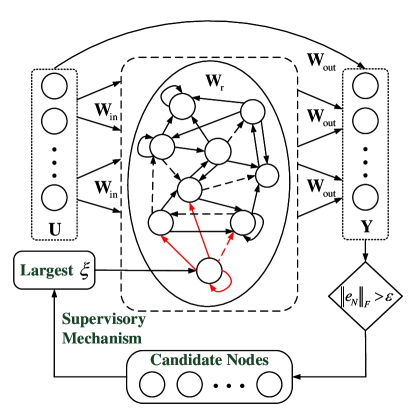
Figure 1: Architecture of the recurrent stochastic configuration network.

Suppose we have built an RSCN with $N$ reservoir nodes, when adding a new node, set the initial state of the new node to zero, ${{\mathbf{x}}_{N+1}}(n-1)=$${{\left[{{x}_{1}}(n-1),\ldots,{{x}_{N}}(n-1),0\right]}^{\top}}$. The reservoir state is

$${{\bf{x}}_{N{\rm{+}}1}}(n)=g\left({{{\bf{W}}_{{\mathop{\rm in}\nolimits},N+1}}{\bf{u}}(n)}\right.+\left.{{{\bf{W}}_{{\mathop{\rm r}\nolimits},N+1}}{{\bf{x}}_{N+1}}(n-1)+{{\bf{b}}_{N+1}}}\right)=g({\bf{x}}_{{\mathop{\rm in}\nolimits},N+1}(n-1)+{\bf{x}}_{{\rm{r}},N+1}(n-1)),$$ (17)

where

$$\begin{array}[]{l}{\bf{W}}_{{\mathop{\rm i}\nolimits}{\mathop{\rm n}\nolimits},N+1}{\bf{u}}(n){\rm{+}}{{\bf{b}}_{N+1}}=\\ \left[{\begin{array}[]{*{20}{c}}{w_{{\mathop{\rm i}\nolimits}{\mathop{\rm n}\nolimits}}^{1,1}}&{w_{{\mathop{\rm i}\nolimits}{\mathop{\rm n}\nolimits}}^{1,2}}&\cdots&{w_{{\mathop{\rm i}\nolimits}{\mathop{\rm n}\nolimits}}^{1,K}}\\ {w_{{\mathop{\rm i}\nolimits}{\mathop{\rm n}\nolimits}}^{2,1}}&{w_{{\mathop{\rm i}\nolimits}{\mathop{\rm n}\nolimits}}^{2,2}}&\cdots&{w_{{\mathop{\rm i}\nolimits}{\mathop{\rm n}\nolimits}}^{2,K}}\\ \vdots&\vdots&\vdots&\vdots\\ {w_{{\mathop{\rm i}\nolimits}{\mathop{\rm n}\nolimits}}^{N,1}}&{w_{{\mathop{\rm i}\nolimits}{\mathop{\rm n}\nolimits}}^{N,2}}&\cdots&{w_{{\mathop{\rm i}\nolimits}{\mathop{\rm n}\nolimits}}^{N,K}}\\ {w_{{\mathop{\rm i}\nolimits}{\mathop{\rm n}\nolimits}}^{N+1,1}}&{w_{{\mathop{\rm i}\nolimits}{\mathop{\rm n}\nolimits}}^{N+1,2}}&\cdots&{w_{{\mathop{\rm i}\nolimits}{\mathop{\rm n}\nolimits}}^{N+1,K}}\end{array}}\right]{\bf{u}}(n)+\left[{\begin{array}[]{*{20}{c}}{{b_{1}}}\\ {{b_{2}}}\\ \vdots\\ {{b_{N}}}\\ {{b_{N+1}}}\end{array}}\right]\\ {\kern 1.0pt}{\rm{=}}{\kern 1.0pt}{\kern 1.0pt}{\bf{x}}_{{\mathop{\rm in}\nolimits},N+1}(n-1)\in{{\mathbb{R}}^{N+1}},\end{array}$$ (18)

$$\begin{array}[]{l}{{\bf{W}}_{{\mathop{\rm r}\nolimits},N+1}}{{\bf{x}}_{N+1}}(n-1){\rm{=}}\\ \left[{\begin{array}[]{*{20}{c}}{w_{\mathop{\rm r}\nolimits}^{1,1}}&0&\cdots&0&0\\ {w_{\mathop{\rm r}\nolimits}^{2,1}}&{w_{\mathop{\rm r}\nolimits}^{2,2}}&\cdots&0&0\\ \vdots&\vdots&\vdots&\vdots&\vdots\\ {w_{\mathop{\rm r}\nolimits}^{N,1}}&{w_{\mathop{\rm r}\nolimits}^{N,2}}&\cdots&{w_{\mathop{\rm r}\nolimits}^{N,N}}&0\\ {w_{\mathop{\rm r}\nolimits}^{N{\rm{+1,1}}}}&{w_{\mathop{\rm r}\nolimits}^{N{\rm{+1,2}}}}&\cdots&{w_{\mathop{\rm r}\nolimits}^{N{\rm{+}}1,N}}&{w_{\mathop{\rm r}\nolimits}^{N{\rm{+}}1,N+1}}\end{array}}\right]\left[{\begin{array}[]{*{20}{c}}{{x_{1}}(n-1)}\\ {{x_{2}}(n-1)}\\ \vdots\\ {{x_{N}}(n-1)}\\ 0\end{array}}\right]\\ {\kern 1.0pt}{\rm{=}}{\left[{x_{1}\left({n-1}\right),...,x_{N}\left({n-1}\right),x_{N+1}\left({n-1}\right)}\right]^{\top}}{\rm{=}}{\kern 1.0pt}{\kern 1.0pt}{\kern 1.0pt}{\kern 1.0pt}{\bf{x}}_{{\rm{r}},N+1}(n-1)\in{{\mathbb{R}}^{N+1}}.\end{array}$$ (19)

Given the input signals $\mathbf{U}\text{=}\left[\mathbf{u}(1),\mathbf{u}(2),\ldots,\mathbf{u}({{n}_{\max}})\right]$, the error between the model output and the desired output is $e_{N}=\mathbf{Y}-\mathbf{T}$. When ${{\left\|{{e}_{N}}\right\|}_{F}}$ does not meet the preset threshold, it is necessary to add nodes under the supervisory mechanism. Seek the random basis function ${g_{N{\rm{+}}1}}$ satisfying the following inequality

$${\left\langle{e_{N,q},{g_{N{\rm{+}}1}}}\right\rangle^{2}}\geq b_{g}^{2}(1-r-{\mu_{N+1}})\left\|{{e_{N,q}}}\right\|^{2},q=1,2,...L,$$ (20)

where $\left\{{{\mu}_{N+1}}\right\}$ is a nonnegative real sequence that satisfies $\underset{N\to\infty}{\mathop{\lim}}\,{{\mu}_{N+1}}=0$ and ${{\mu}_{N+1}}\leq(1-r)$, $0<\left\|g\right\|<{{b}_{g}}$. In addition, to facilitate the implementation of RSCNs, ${\xi_{N+1,q}}$ is calculated for each candidate node according to Eq. (11). And the candidate node with the largest ${{\xi}_{N+1}}=\sum\limits_{q=1}^{L}{{{\xi}_{N+1,q}}}$ is determined as the optimal adding node. Then, the output weight is determined by the global least square method

$${{\bf{W}}_{{\rm{out}},N{\rm{+}}1}{\rm{=}}\left[{{\bf{w}}_{{\rm{out}},1},{\bf{w}}_{{\rm{out}},2},...,{\bf{w}}_{{\rm{out}},N+1+K}}\right]=\mathop{\arg\min}\limits_{{\bf{W}}_{{\rm{out}},N+1}}\left\|{{\bf{T}}-{\bf{W}}_{{\rm{out}},N+1}{{\bf{X}}_{N+1}}}\right\|^{2},}$$ (21)

where ${{\mathbf{X}}_{N+1}}\text{=}\left[\left({{\mathbf{x}}_{N+1}}\left(1\right),\mathbf{u}\left(1\right)\right),\ldots,\left({{\mathbf{x}}_{N+1}}\left({{n}_{\max}}\right),\mathbf{u}\left({{n}_{\max}}\right)\right)\right]$. Calculate the residual error ${{e}_{N+1}}$ and update $N=N+1$. Continue to add nodes until ${{\left\|e\right\|}_{F}}<\varepsilon$ or $N\geq{{N}_{\max}}$, where ${{N}_{\max}}$ is the maximum reservoir size. Finally, we have $\underset{N\to\infty}{\mathop{\lim}}\,{{\left\|{{e}_{N}}\right\|}_{F}}=0$. The construction process of RSCNs is summarized in Algorithm 1.

Input: Given inputs $\mathbf{U}\text{=}\left[\mathbf{u}(1),\mathbf{u}(2),\ldots,\mathbf{u}({{n}_{\max}})\right]$, outputs ${\bf{T}}={\left[{{\bf{t}}\left(1\right),\ldots,{\bf{t}}\left({{n_{max}}}\right)}\right]}$, initial reservoir size $N$, the maximum reservoir size ${N_{\max}}$, training error threshold $\varepsilon$, positive scalars $\mathbf{\gamma}\text{=}\left\{{{\lambda}_{\min}},{{\lambda}_{\min}}+\Delta\lambda,...,{{\lambda}_{\max}}\right\}$, and the maximum number of stochastic configurations ${{G}_{\max}}$.

1 Initialization: Randomly assign ${{\mathbf{W}}_{\operatorname{in},N}}$, ${{\bf{b}}_{N}}$, and ${{\mathbf{W}}_{\rm r,N}}$ according to the sparsity of the reservoir from $\left[-\lambda,\lambda\right]$, and calculate the model output $\mathbf{Y}$ and current error ${e}_{N}$, let ${{e}_{0}}={{e}_{N}}$, $0<r<1$, $\mathbf{\Omega},\mathbf{D}:=\left[{\kern 1.0pt}{\kern 1.0pt}{\kern 1.0pt}\right]$.

2 while $N\leq{{N}_{\text{max}}}$ AND ${{\left\|e_{0}\right\|}_{F}}>\varepsilon$, do

3       Phase 1: Reservoir Parameter Configuration (Step 4-26)

4       for $\lambda\in\mathbf{\gamma}$ do

5             for $k=1,2,...,{{G}_{\max}}$ do

6                   Randomly assign ${b_{N+1}}$, ${\bf{w}}_{{\mathop{\rm i}\nolimits}{\mathop{\rm n}\nolimits}}^{N+1}=\left[\begin{matrix}w_{\operatorname{i}\operatorname{n}}^{N+1,1}&\cdots&w_{\operatorname{i}\operatorname{n}}^{N+1,K}\end{matrix}\right],$ and ${\bf{w}}_{{\mathop{\rm r}\nolimits}}^{N+1}=\left[\begin{matrix}w_{\operatorname{r}}^{N+1,1}&\cdots&w_{\operatorname{r}}^{N+1,N+1}\end{matrix}\right]$ from $\left[-\lambda,\lambda\right]$;

7                   Construct $\mathbf{W}_{\operatorname{i}\operatorname{n},N+1}$ and $\mathbf{W}_{\text{r},N+1}$;

8                   Calculate $\mathbf{x}_{\operatorname{in},N+1}(n-1)$ and $\mathbf{x}_{\text{r},N+1}(n-1)$ based on Eq. (18) and Eq. (19);

9                   Calculate ${{g}_{N+1}}$ and ${{\xi}_{N\text{+}1,q}}$;

10                   Set ${{\mu}_{N\text{+}1}}\text{=}(1-r)/\left(N\text{+}K\right)$;

11                   if $\min\left\{{{\xi}_{N\text{+}1,1}},{{\xi}_{N\text{+}1,2}},...,{{\xi}_{N\text{+1},L}}\right\}\geq 0$ then

12                         Save $\mathbf{w}_{\operatorname{i}\operatorname{n}}^{N+1},$ ${{b}_{N+1}}$ and $\mathbf{w}_{\text{r}}^{N+1}$ in $\mathbf{D}$, $\xi_{N\text{+}1}\text{=}\sum\limits_{q=1}^{L}{{{\xi}_{N\text{+}1,q}}}$ in $\mathbf{\Omega}$;

13                         else

14                              go back to Step 5

15                         end if

16                        

17                   end if

18                  

19             end for

20            if $\mathbf{D}$ is not empty then

21                   Find $\mathbf{w}_{\operatorname{i}\operatorname{n}}^{\left(N+1\right)*}$, $b_{N+1}^{*}$, and $\mathbf{w}_{\text{r}}^{\left(N+1\right)*}$ that maximize $\xi_{N\text{+}1}$ in $\mathbf{\Omega}$, construct $\mathbf{W}_{\text{in},N+1}^{*}$, $\mathbf{W}_{\text{r},N+1}^{*}$, and $\mathbf{b}_{N+1}^{*}$, calculate $g_{N+1}^{*}$, and get ${{\mathbf{X}}_{N\text{+}1}}$;

22                   Break (go to Step 28)

23                   else

24                        randomly take $\tau\in\left(0,1-r\right)$, update $r=r+\tau$;

25                   end if

26                  return to Step 5；

27             end if

28            

29       end for

30      Phase 2: Output Weights Determination

31       Calculate $\mathbf{W}_{\operatorname{out},N\text{+}1}^{*}$ according to Eq. (21);

32       Calculate $e_{N\text{+}1}\text{=}e_{N}-\mathbf{w}_{\operatorname{out},N+1}^{*}g_{N+1}^{*}$;

33       Update ${{e}_{0}}:=e_{N+1}$, $N:=N+1$;

34 end while

Return: $\mathbf{W}_{\text{in},N}^{*}=\left\{\mathbf{w}_{\text{in}}^{\left(1\right)*},\ldots,\mathbf{w}_{\text{in}}^{\left(N\right)*}\right\}$, $\mathbf{b}_{N}^{*}=\left\{b_{1}^{*},\ldots,b_{N}^{*}\right\}$, $\mathbf{W}_{\text{r},N}^{*}$, and $\mathbf{W}_{\text{out},N}^{*}$.

Algorithm 1 Recurrent stochastic configuration (RSC)

Remark 2

The model output can be regarded as a linear combination of reservoir output and input direct link. We can obtain the globally optimal $\mathbf{W}_{\text{out}}$ using the least squares method. Further research is necessary for the system that requires precise calculation of the individual weights corresponding to two components.

3.2 The echo state property of RSCN

The echo state property is an intrinsic characteristic that distinguishes ESN from other networks. As the length of the input sequence approaches infinity, the error between two reservoir states ${\bf{x}}^{1}\left(n\right)$ and ${\bf{x}}^{2}\left(n\right)$, driven by the same input sequence but starting from different initial conditions, tends to zero. And the dependence of ${\bf{x}}\left(n\right)$ on the initial state ${\bf{x}}\left(0\right)$ diminishes over time, indicating that the current state only relies on historical inputs and is independent of the initial state.

Let ${{\sigma}_{\max}}\left({{\mathbf{W}}_{\text{r}}}\right)$ denote the maximal singular value of ${{\mathbf{W}}_{\text{r}}}$. The spectral radius of ${{\mathbf{W}}_{\text{r}}}$ is set to $\rho\left({{\mathbf{W}}_{\text{r}}}\right)=\max\left(\left|{{\theta}_{1}}\right|,\left|{{\theta}_{2}}\right|,\ldots\right)$, where ${{\theta}_{i}}$ is the eigenvalue of ${{\mathbf{W}}_{\text{r}}}$. Observe that the largest singular value of ${{\mathbf{W}}_{\text{r}}}$ can be scaled with $\alpha$, that is, ${{\sigma}_{\max}}\left(\alpha{{\mathbf{W}}_{\text{r}}}\right)=\alpha{{\sigma}_{\max}}\left({{\mathbf{W}}_{\text{r}}}\right)$. It can be further inferred that for each square matrix ${{\mathbf{W}}_{\text{r}}}$, and $\rho\left({{\mathbf{W}}_{\text{r}}}\right)\leq{{\sigma}_{\max}}\left({{\mathbf{W}}_{\text{r}}}\right)$. The feedback matrix can be rewritten as

$${{\bf{W}}_{{\rm{r}},{{N+1}}}}\leftarrow\frac{\alpha}{{\rho\left({{{\bf{W}}_{{\rm{r}},{{N+1}}}}}\right)}}{{\bf{W}}_{{\rm{r}},{{N+1}}}},$$ (22)

where $0<\alpha<1$ represents the scaling factor. Substitute ${{\bf{W}}_{{{r,N+1}}}}$ obtained from Eq. (15) into Eq. (22) and seek for the nodes that satisfy the inequality constraints in Eq. (20). The echo state property of RSCN is guaranteed if $\alpha$ is chosen as

$$0<\alpha<\frac{{\rho\left({{{\bf{W}}_{{\rm{r}},{{N+1}}}}}\right)}}{{{\sigma_{\max}}\left({{{\bf{W}}_{{\rm{r}},{{N+1}}}}}\right)}}.$$ (23)

Proof. Randomly assign two initial states ${\bf{x}}_{N+1}^{1}\left(0\right)$ and ${\bf{x}}_{N+1}^{2}\left(0\right)$. After the system evolves for a period of time, the difference between the reservoir states is

$$\begin{array}[]{l}{\left\|{{\bf{x}}_{N+1}^{1}\left(n\right)-{\bf{x}}_{N+1}^{2}\left(n\right)}\right\|^{2}}=\left\|{g({{\bf{W}}_{{\rm{in}},N+1}}{\bf{u}}(n)+{{\bf{W}}_{{\rm{r}},N+1}}{\bf{x}}_{N+1}^{1}(n-1)+{{\bf{b}}_{N+1}})}\right.\\ {\kern 1.0pt}{\kern 1.0pt}{\kern 1.0pt}{\kern 1.0pt}{\kern 1.0pt}{\kern 1.0pt}{\kern 1.0pt}{\kern 1.0pt}{\kern 1.0pt}{\kern 1.0pt}{\kern 1.0pt}{\kern 1.0pt}{\kern 1.0pt}{\kern 1.0pt}{\kern 1.0pt}{\kern 1.0pt}{\kern 1.0pt}{\kern 1.0pt}{\kern 1.0pt}{\kern 1.0pt}{\kern 1.0pt}{\kern 1.0pt}{\kern 1.0pt}{\kern 1.0pt}{\kern 1.0pt}{\kern 1.0pt}{\kern 1.0pt}{\kern 1.0pt}{\kern 1.0pt}{\kern 1.0pt}{\kern 1.0pt}{\kern 1.0pt}{\kern 1.0pt}{\kern 1.0pt}{\kern 1.0pt}{\kern 1.0pt}{\kern 1.0pt}{\kern 1.0pt}{\kern 1.0pt}{\kern 1.0pt}{\kern 1.0pt}{\kern 1.0pt}{\kern 1.0pt}{\kern 1.0pt}{\kern 1.0pt}{\kern 1.0pt}{\kern 1.0pt}{\kern 1.0pt}{\kern 1.0pt}{\kern 1.0pt}{\kern 1.0pt}{\kern 1.0pt}{\kern 1.0pt}{\kern 1.0pt}{\kern 1.0pt}{\kern 1.0pt}{\kern 1.0pt}{\kern 1.0pt}{\kern 1.0pt}{\kern 1.0pt}{\kern 1.0pt}{\kern 1.0pt}{\kern 1.0pt}{\kern 1.0pt}{\kern 1.0pt}{\kern 1.0pt}{\kern 1.0pt}{\kern 1.0pt}{\kern 1.0pt}{\kern 1.0pt}{\kern 1.0pt}{\kern 1.0pt}{\kern 1.0pt}{\kern 1.0pt}{\kern 1.0pt}{\kern 1.0pt}{\kern 1.0pt}{\kern 1.0pt}{\kern 1.0pt}{\kern 1.0pt}{\kern 1.0pt}{\kern 1.0pt}{\kern 1.0pt}{\kern 1.0pt}{\kern 1.0pt}{\kern 1.0pt}{\kern 1.0pt}{\kern 1.0pt}{\kern 1.0pt}{\kern 1.0pt}{\kern 1.0pt}{\kern 1.0pt}{\kern 1.0pt}{\kern 1.0pt}{\kern 1.0pt}{\kern 1.0pt}{\kern 1.0pt}{\kern 1.0pt}{\kern 1.0pt}{\kern 1.0pt}{\kern 1.0pt}{\kern 1.0pt}{\kern 1.0pt}{\kern 1.0pt}{\kern 1.0pt}{\kern 1.0pt}{\kern 1.0pt}{\kern 1.0pt}{\kern 1.0pt}{\kern 1.0pt}{\kern 1.0pt}-{\left.{g({{\bf{W}}_{{\rm{in}},N+1}}{\bf{u}}(n)+{{\bf{W}}_{{\rm{r}},N+1}}{\bf{x}}_{N+1}^{2}(n-1)+{{\bf{b}}_{N+1}})}\right\|^{2}},\end{array}$$ (24)

where $g$ is the sigmoid or tanh function. According to the Lipschitz condition, we have

$$\begin{array}[]{l}{\left\|{{\bf{x}}_{N+1}^{1}\left(n\right)-{\bf{x}}_{N+1}^{2}\left(n\right)}\right\|^{2}}\leq\max\left({\left|{g^{\prime}}\right|}\right){\left\|{{{\bf{W}}_{{\rm{r}},N+1}}{\bf{x}}_{N+1}^{1}(n-1)-{{\bf{W}}_{{\rm{r}},N+1}}{\bf{x}}_{N+1}^{2}(n-1)}\right\|^{2}}\\ \leq\left\|{{{\bf{W}}_{{\rm{r}},N+1}}}\right\|{\left\|{{\bf{x}}_{N+1}^{1}\left({n-1}\right)-{\bf{x}}_{N+1}^{2}\left({n-1}\right)}\right\|^{2}}\leq\left\|{{{\bf{W}}_{{\rm{r}},N+1}}}\right\|^{2}{\left\|{{\bf{x}}_{N+1}^{1}\left({n-2}\right)-{\bf{x}}_{N+1}^{2}\left({n-2}\right)}\right\|^{2}}\\ \leq\ldots\leq\left\|{{{\bf{W}}_{{\rm{r}},N+1}}}\right\|^{n}{\left\|{{\bf{x}}_{N+1}^{1}\left(0\right)-{\bf{x}}_{N+1}^{2}\left(0\right)}\right\|^{2}},\end{array}$$ (25)

where ${g^{\prime}}$ is the first order derivative of $g$. Observe that

$$\begin{array}[]{l}{\sigma_{\max}}\left({\frac{\alpha}{{\rho\left({{{\bf{W}}_{{\rm{r}},N{\rm{+1}}}}}\right)}}{{\bf{W}}_{{\rm{r}},N{\rm{+1}}}}}\right)=\frac{\alpha}{{\rho\left({{{\bf{W}}_{{\rm{r}},N{\rm{+1}}}}}\right)}}{\sigma_{\max}}\left({{{\bf{W}}_{{\rm{r}},N{\rm{+1}}}}}\right)<\frac{{\rho\left({{{\bf{W}}_{{\rm{r}},N{\rm{+1}}}}}\right)}}{{{\sigma_{\max}}\left({{{\bf{W}}_{{\rm{r}},N{\rm{+1}}}}}\right)}}\times\frac{1}{{\rho\left({{{\bf{W}}_{{\rm{r}},N{\rm{+1}}}}}\right)}}{\sigma_{\max}}\left({{{\bf{W}}_{{\rm{r}},N{\rm{+1}}}}}\right)=1.\end{array}$$ (26)

Since the Euclidean norm of the matrix is equal to the maximum singular value, we have $\left\|{{\mathbf{W}}_{\text{r},N+1}}\right\|<1$ and $\underset{n\to\infty}{\mathop{\lim}}\,\left\|{{\mathbf{W}}_{\operatorname{r},N+1}}\right\|^{n}=0$. It can be easily obtained that $\underset{n\to\infty}{\mathop{\lim}}\,\left\|\mathbf{x}_{N+1}^{1}\left(n\right)-\mathbf{x}_{N+1}^{2}\left(n\right)\right\|=0,$ which completes the proof.

3.3 Online learning of parameters

Due to the dynamic changes in the actual industrial process, it is essential to update the model parameters online. The network model is known to be

$${\bf{\hat{x}}}(n)=g({{\bf{\hat{W}}}_{{\rm{in}}}}{\bf{u}}(n)+{{\bf{\hat{W}}}_{\mathop{\rm r}\nolimits}}{\bf{\hat{x}}}(n-1){\rm{+}}{\bf{\hat{b}}}),$$ (27)

$${\bf{\hat{y}}}(n)={{\bf{\hat{W}}}_{\rm{out}}}\left({{\bf{\hat{x}}}(n),{\bf{u}}(n)}\right),$$ (28)

where $\mathbf{\hat{x}}(n),\mathbf{\hat{y}}(n)$ are the predicted state vectors and output. ${{\mathbf{\hat{W}}}_{\text{in}}},{{\mathbf{\hat{W}}}_{\operatorname{r}}}$ are the trained input weight matrix and feedback matrix, respectively, which do not adjust anymore. Let $\mathbf{\hat{g}}(n)=\left(\mathbf{\hat{x}}(n),\mathbf{u}(n)\right)$, and the projection algorithm is used to update the output weights ${{\mathbf{\hat{W}}}_{\rm{out}}}$.

Theorem 1 [28]. In the hyperplane ${\rm{H}}=\left\{{{{\mathbf{\hat{W}}}}_{\rm{out}}}:\mathbf{\hat{y}}(n)={{{\mathbf{\hat{W}}}}_{\rm{out}}}\mathbf{\hat{g}}(n)\right\}$, choose the weight closest to ${{\mathbf{\hat{W}}}_{\rm{out}}}\left(n-1\right)$ as ${{\mathbf{\hat{W}}}_{\rm{out}}}\left(n\right)$. Given ${{\mathbf{\hat{W}}}_{\rm{out}}}\left(n-1\right)$ and $\mathbf{y}\left(n\right)$, determine ${{\mathbf{\hat{W}}}_{\rm{out}}}\left(n\right)$ to minimize the cost function

$$\begin{array}[]{*{20}{c}}{J=\frac{1}{2}{{\left\|{{{{\bf{\hat{W}}}}_{\rm{out}}}\left(n\right)-{{{\bf{\hat{W}}}}_{\rm{out}}}\left({n-1}\right)}\right\|}^{2}}}\\ {s.t.{\kern 1.0pt}{\kern 1.0pt}{\kern 1.0pt}{\kern 1.0pt}{\kern 1.0pt}{\kern 1.0pt}{\kern 1.0pt}{\kern 1.0pt}{\kern 1.0pt}{\kern 1.0pt}{\bf{y}}\left(n\right)={{{\bf{\hat{W}}}}_{\rm{out}}}\left(n\right){\bf{\hat{g}}}(n)}\end{array}.$$ (29)

By introducing the Lagrange operator ${{\lambda}_{\text{p}}}$, we can obtain

$${J_{e}}=\frac{1}{2}{\left\|{{{{\bf{\hat{W}}}}_{\rm{out}}}\left(n\right)-{{{\bf{\hat{W}}}}_{\rm{out}}}\left({n-1}\right)}\right\|^{2}}+{\lambda_{\rm{p}}}\left({{\bf{y}}\left(n\right)-{{{\bf{\hat{W}}}}_{\rm{out}}}\left(n\right){\bf{\hat{g}}}(n)}\right).$$ (30)

The necessary conditions for ${{J}_{e}}$ to be minimal are

$$\left\{{\begin{array}[]{*{20}{c}}{\frac{{\partial{J_{e}}}}{{\partial{{{\bf{\hat{W}}}}_{\rm{out}}}\left(n\right)}}=0}\\ {\frac{{\partial{J_{e}}}}{{\partial{\lambda_{\rm{p}}}}}=0}\end{array}}\right..$$ (31)

Then, we have

$$\left\{{\begin{array}[]{*{20}{c}}{{{{\bf{\hat{W}}}}_{\rm{out}}}\left(n\right)-{{{\bf{\hat{W}}}}_{\rm{out}}}\left({n-1}\right)-{\lambda_{\rm{p}}}{{{\bf{\hat{g}}}}^{\top}}(n)=0}\\ {{\bf{y}}\left(n\right)-{{{\bf{\hat{W}}}}_{\rm{out}}}\left(n\right){\bf{\hat{g}}}(n)=0}\end{array}}\right.,$$ (32)

$${\lambda_{\rm{p}}}=\frac{{{\bf{y}}\left(n\right)-{{{\bf{\hat{W}}}}_{\rm{out}}}\left({n-1}\right){\bf{\hat{g}}}(n)}}{{{\bf{\hat{g}}}{{(n)}^{\top}}{\bf{\hat{g}}}(n)}}.$$ (33)

Substituting Eq. (33) into Eq. (32), yields

$${{\bf{\hat{W}}}_{\rm{out}}}(n)={{\bf{\hat{W}}}_{\rm{out}}}(n-1)+\frac{{{\bf{\hat{g}}}{{(n)}^{\top}}}}{{{\bf{\hat{g}}}{{(n)}^{\top}}{\bf{\hat{g}}}(n)}}\left({{\bf{y}}\left(n\right)-{{{\bf{\hat{W}}}}_{\rm{out}}}\left({n-1}\right){\bf{\hat{g}}}(n)}\right).$$ (34)

To avoid division by zero, a small constant $c$ is added to the denominator. Moreover, a coefficient $a$ is multiplied by the numerator to obtain the improved projection algorithm

$${{\bf{\hat{W}}}_{\rm{out}}}(n)={{\bf{\hat{W}}}_{\rm{out}}}(n-1)+\frac{{a{\bf{\hat{g}}}{{(n)}^{\top}}}}{{c+{\bf{\hat{g}}}{{(n)}^{\top}}{\bf{\hat{g}}}(n)}}\left({{\bf{y}}\left(n\right)-{{{\bf{\hat{W}}}}_{\rm{out}}}\left({n-1}\right){\bf{\hat{g}}}(n)}\right),$$ (35)

where $0<a\leq 1$ and $c>0$.

Input: Given the input $\left[\mathbf{u}(1),\mathbf{u}(2),\ldots,\mathbf{u}(n)\right]$, the output $\left[\mathbf{y}\left(1\right),\ldots,\mathbf{y}\left(n\right)\right]$, initial state $\mathbf{\hat{x}}(0)$, offline trained input weight matrix ${{\mathbf{\hat{W}}}_{\text{in}}}$, feedback matrix ${{\mathbf{\hat{W}}}_{\operatorname{r}}}$, output weights ${{\mathbf{\hat{W}}}_{\text{out}}}$, and constants $a,c.$

1 Initialization: Assign output weights for the initial moment ${{\mathbf{\hat{W}}}_{\rm{out}}}(1)\text{=}{{\mathbf{\hat{W}}}_{\text{out}}};$

2 Input the samples sequentially into Eq. (27) and obtain $\left[\mathbf{\hat{x}}(1),\ldots,\mathbf{\hat{x}}(n)\right],$ $\left[\mathbf{\hat{g}}(1),\ldots,\mathbf{\hat{g}}(n)\right]$;

3 Calculate the output of the first step $\mathbf{\hat{y}}(1)={{\mathbf{\hat{W}}}_{\rm{out}}}\left(1\right)\mathbf{\hat{g}}(1)$;

4 for $i=2,3,\ldots,n,$ do

5       Update ${{\mathbf{\hat{W}}}_{\rm{out}}}(i)$ according to Eq. (35);

6       Calculate $\mathbf{\hat{y}}(i)={{\mathbf{\hat{W}}}_{\rm{out}}}\left(i\right)\mathbf{\hat{g}}(i)$;

7 end for

Return: $\left[{{{\mathbf{\hat{W}}}}_{\rm{out}}}\left(1\right),\ldots,{{{\mathbf{\hat{W}}}}_{\rm{out}}}\left(n\right)\right]$.

Algorithm 2 Projection algorithm for updating output weights

3.4 The universal approximation property for offline learning

Theorem 2. Suppose that span($\Gamma$) is dense in ${{L}_{2}}$ space, for $b_{g}\in{{\mathbb{R}}^{+}}$ , $\forall g\in\Gamma,0<\left\|g\right\|<{{b}_{g}}$. Given $0<r<1$ and a nonnegative real sequence $\left\{{{\mu}_{N+1}}\right\}$ satisfies $\underset{N\to\infty}{\mathop{\lim}}\,{{\mu}_{N\text{+}1}}=0$ and ${{\mu}_{N\text{+}1}}\leq(1-r)$. For $N=1,2...$, $q=1,2,...,L$, define

$${\delta_{N{\rm{+1}}}}=\sum\limits_{q=1}^{L}{\delta_{N{\rm{+}}1,q}}{\kern 1.0pt}{\kern 1.0pt}{\kern 1.0pt}{\kern 1.0pt},{\kern 1.0pt}{\kern 1.0pt}{\kern 1.0pt}\delta_{N{\rm{+}}1,q}=(1-r-{\mu_{N{\rm{+}}1}})\left\|{e_{N,q}}\right\|^{2}.$$ (36)

If $g_{N\text{+}1}$ satisfies the following inequality constraints

$${\left\langle{e_{N,q},{g_{N{\rm{+}}1}}}\right\rangle^{2}}\geq b_{g}^{2}\delta_{N{\rm{+}}1,q},q=1,2,...L,$$ (37)

and the output weight is constructively evaluated by

$${\bf{w}}_{{\mathop{\rm out}\nolimits},N+1,q}^{*}=\frac{{\left\langle{e_{N,q},g_{N{\rm{+}}1}}\right\rangle}}{{\left\|{g_{N{\rm{+}}1}}\right\|^{2}}},q=1,2,...,L,$$ (38)

we have ${{\lim}_{N\to\infty}}\left\|e_{N\text{+}1}\right\|=0$.

Proof. With simple computation, we have

$$\begin{array}[]{l}\left\|{e_{N{\rm{+}}1}}\right\|^{2}-\left({r+{\mu_{N{\rm{+}}1}}}\right)\left\|{e_{N}}\right\|^{2}{\kern 1.0pt}=\sum\limits_{q=1}^{L}{\left\langle{e_{N,q}-{\bf{w}}_{{\mathop{\rm out}\nolimits},N+1}^{*}g_{N+1},e_{N,q}-{\bf{w}}_{{\mathop{\rm out}\nolimits},N+1}^{*}g_{N+1}}\right\rangle}\\ {\kern 1.0pt}{\kern 1.0pt}{\kern 1.0pt}{\kern 1.0pt}{\kern 1.0pt}{\kern 1.0pt}{\kern 1.0pt}{\kern 1.0pt}{\kern 1.0pt}{\kern 1.0pt}{\kern 1.0pt}{\kern 1.0pt}{\kern 1.0pt}{\kern 1.0pt}{\kern 1.0pt}{\kern 1.0pt}{\kern 1.0pt}{\kern 1.0pt}{\kern 1.0pt}{\kern 1.0pt}{\kern 1.0pt}{\kern 1.0pt}{\kern 1.0pt}{\kern 1.0pt}{\kern 1.0pt}{\kern 1.0pt}{\kern 1.0pt}{\kern 1.0pt}{\kern 1.0pt}{\kern 1.0pt}{\kern 1.0pt}{\kern 1.0pt}{\kern 1.0pt}{\kern 1.0pt}{\kern 1.0pt}{\kern 1.0pt}{\kern 1.0pt}{\kern 1.0pt}{\kern 1.0pt}{\kern 1.0pt}{\kern 1.0pt}{\kern 1.0pt}{\kern 1.0pt}{\kern 1.0pt}{\kern 1.0pt}{\kern 1.0pt}{\kern 1.0pt}{\kern 1.0pt}{\kern 1.0pt}{\kern 1.0pt}{\kern 1.0pt}{\kern 1.0pt}{\kern 1.0pt}{\kern 1.0pt}{\kern 1.0pt}{\kern 1.0pt}{\kern 1.0pt}{\kern 1.0pt}{\kern 1.0pt}{\kern 1.0pt}{\kern 1.0pt}{\kern 1.0pt}{\kern 1.0pt}{\kern 1.0pt}{\kern 1.0pt}{\kern 1.0pt}{\kern 1.0pt}{\kern 1.0pt}{\kern 1.0pt}{\kern 1.0pt}{\kern 1.0pt}{\kern 1.0pt}{\kern 1.0pt}{\kern 1.0pt}{\kern 1.0pt}{\kern 1.0pt}{\kern 1.0pt}{\kern 1.0pt}{\kern 1.0pt}{\kern 1.0pt}{\kern 1.0pt}{\kern 1.0pt}{\kern 1.0pt}{\kern 1.0pt}{\kern 1.0pt}{\kern 1.0pt}{\kern 1.0pt}{\kern 1.0pt}{\kern 1.0pt}{\kern 1.0pt}{\kern 1.0pt}{\kern 1.0pt}{\kern 1.0pt}{\kern 1.0pt}{\kern 1.0pt}{\kern 1.0pt}{\kern 1.0pt}{\kern 1.0pt}{\kern 1.0pt}{\kern 1.0pt}{\kern 1.0pt}{\kern 1.0pt}{\kern 1.0pt}{\kern 1.0pt}{\kern 1.0pt}{\kern 1.0pt}{\kern 1.0pt}{\kern 1.0pt}{\kern 1.0pt}{\kern 1.0pt}{\kern 1.0pt}{\kern 1.0pt}{\kern 1.0pt}{\kern 1.0pt}{\kern 1.0pt}{\kern 1.0pt}{\kern 1.0pt}{\kern 1.0pt}{\kern 1.0pt}{\kern 1.0pt}{\kern 1.0pt}{\kern 1.0pt}{\kern 1.0pt}{\kern 1.0pt}{\kern 1.0pt}{\kern 1.0pt}{\kern 1.0pt}{\kern 1.0pt}{\kern 1.0pt}{\kern 1.0pt}{\kern 1.0pt}{\kern 1.0pt}{\kern 1.0pt}{\kern 1.0pt}-\sum\limits_{q=1}^{L}{\left({r+{\mu_{N{\rm{+}}1}}}\right)\left\langle{e_{N,q},e_{N,q}}\right\rangle}\\ {\kern 1.0pt}{\kern 1.0pt}{\kern 1.0pt}{\kern 1.0pt}{\kern 1.0pt}{\kern 1.0pt}{\kern 1.0pt}{\kern 1.0pt}{\kern 1.0pt}{\kern 1.0pt}{\kern 1.0pt}{\kern 1.0pt}{\kern 1.0pt}{\kern 1.0pt}{\kern 1.0pt}{\kern 1.0pt}{\kern 1.0pt}{\kern 1.0pt}{\kern 1.0pt}{\kern 1.0pt}{\kern 1.0pt}{\kern 1.0pt}{\kern 1.0pt}{\kern 1.0pt}{\kern 1.0pt}{\kern 1.0pt}{\kern 1.0pt}{\kern 1.0pt}{\kern 1.0pt}{\kern 1.0pt}{\kern 1.0pt}{\kern 1.0pt}{\kern 1.0pt}{\kern 1.0pt}{\kern 1.0pt}{\kern 1.0pt}{\kern 1.0pt}{\kern 1.0pt}{\kern 1.0pt}{\kern 1.0pt}{\kern 1.0pt}{\kern 1.0pt}{\kern 1.0pt}{\kern 1.0pt}{\kern 1.0pt}{\kern 1.0pt}{\kern 1.0pt}{\kern 1.0pt}{\kern 1.0pt}{\kern 1.0pt}{\kern 1.0pt}{\kern 1.0pt}{\kern 1.0pt}{\kern 1.0pt}{\kern 1.0pt}{\kern 1.0pt}{\kern 1.0pt}{\kern 1.0pt}{\kern 1.0pt}{\kern 1.0pt}{\kern 1.0pt}{\kern 1.0pt}{\kern 1.0pt}{\kern 1.0pt}{\kern 1.0pt}{\kern 1.0pt}{\kern 1.0pt}{\kern 1.0pt}{\kern 1.0pt}{\kern 1.0pt}{\kern 1.0pt}{\kern 1.0pt}{\kern 1.0pt}{\kern 1.0pt}{\kern 1.0pt}{\kern 1.0pt}{\kern 1.0pt}{\kern 1.0pt}{\kern 1.0pt}{\kern 1.0pt}{\kern 1.0pt}{\kern 1.0pt}{\kern 1.0pt}{\kern 1.0pt}{\kern 1.0pt}{\kern 1.0pt}{\kern 1.0pt}{\kern 1.0pt}{\kern 1.0pt}{\kern 1.0pt}{\kern 1.0pt}{\kern 1.0pt}{\kern 1.0pt}{\kern 1.0pt}{\kern 1.0pt}{\kern 1.0pt}{\kern 1.0pt}{\kern 1.0pt}{\kern 1.0pt}{\kern 1.0pt}{\kern 1.0pt}{\kern 1.0pt}{\kern 1.0pt}{\kern 1.0pt}{\kern 1.0pt}{\kern 1.0pt}{\kern 1.0pt}{\kern 1.0pt}{\kern 1.0pt}{\kern 1.0pt}{\kern 1.0pt}{\kern 1.0pt}{\kern 1.0pt}{\kern 1.0pt}{\kern 1.0pt}{\kern 1.0pt}{\kern 1.0pt}{\kern 1.0pt}{\kern 1.0pt}{\kern 1.0pt}{\kern 1.0pt}{\kern 1.0pt}{\kern 1.0pt}{\kern 1.0pt}{\kern 1.0pt}{\kern 1.0pt}{\kern 1.0pt}{\kern 1.0pt}{\kern 1.0pt}=\left({1-r-{\mu_{N{\rm{+}}1}}}\right)\left\|{e_{N}}\right\|^{2}-\frac{{\sum\limits_{q=1}^{L}{{{\left\langle{e_{N,q},g_{N+1}}\right\rangle}^{2}}}}}{{\left\|{g_{N+1}}\right\|^{2}}}\\ {\kern 1.0pt}{\kern 1.0pt}{\kern 1.0pt}{\kern 1.0pt}{\kern 1.0pt}{\kern 1.0pt}{\kern 1.0pt}{\kern 1.0pt}{\kern 1.0pt}{\kern 1.0pt}{\kern 1.0pt}{\kern 1.0pt}{\kern 1.0pt}{\kern 1.0pt}{\kern 1.0pt}{\kern 1.0pt}{\kern 1.0pt}{\kern 1.0pt}{\kern 1.0pt}{\kern 1.0pt}{\kern 1.0pt}{\kern 1.0pt}{\kern 1.0pt}{\kern 1.0pt}{\kern 1.0pt}{\kern 1.0pt}{\kern 1.0pt}{\kern 1.0pt}{\kern 1.0pt}{\kern 1.0pt}{\kern 1.0pt}{\kern 1.0pt}{\kern 1.0pt}{\kern 1.0pt}{\kern 1.0pt}{\kern 1.0pt}{\kern 1.0pt}{\kern 1.0pt}{\kern 1.0pt}{\kern 1.0pt}{\kern 1.0pt}{\kern 1.0pt}{\kern 1.0pt}{\kern 1.0pt}{\kern 1.0pt}{\kern 1.0pt}{\kern 1.0pt}{\kern 1.0pt}{\kern 1.0pt}{\kern 1.0pt}{\kern 1.0pt}{\kern 1.0pt}{\kern 1.0pt}{\kern 1.0pt}{\kern 1.0pt}{\kern 1.0pt}{\kern 1.0pt}{\kern 1.0pt}{\kern 1.0pt}{\kern 1.0pt}{\kern 1.0pt}{\kern 1.0pt}{\kern 1.0pt}{\kern 1.0pt}{\kern 1.0pt}{\kern 1.0pt}{\kern 1.0pt}{\kern 1.0pt}{\kern 1.0pt}{\kern 1.0pt}{\kern 1.0pt}{\kern 1.0pt}{\kern 1.0pt}{\kern 1.0pt}{\kern 1.0pt}{\kern 1.0pt}{\kern 1.0pt}{\kern 1.0pt}{\kern 1.0pt}{\kern 1.0pt}{\kern 1.0pt}{\kern 1.0pt}{\kern 1.0pt}{\kern 1.0pt}{\kern 1.0pt}{\kern 1.0pt}{\kern 1.0pt}{\kern 1.0pt}{\kern 1.0pt}{\kern 1.0pt}{\kern 1.0pt}{\kern 1.0pt}{\kern 1.0pt}{\kern 1.0pt}{\kern 1.0pt}{\kern 1.0pt}{\kern 1.0pt}{\kern 1.0pt}{\kern 1.0pt}{\kern 1.0pt}{\kern 1.0pt}{\kern 1.0pt}{\kern 1.0pt}{\kern 1.0pt}{\kern 1.0pt}{\kern 1.0pt}{\kern 1.0pt}{\kern 1.0pt}{\kern 1.0pt}{\kern 1.0pt}{\kern 1.0pt}{\kern 1.0pt}{\kern 1.0pt}{\kern 1.0pt}{\kern 1.0pt}{\kern 1.0pt}{\kern 1.0pt}{\kern 1.0pt}{\kern 1.0pt}{\kern 1.0pt}{\kern 1.0pt}{\kern 1.0pt}{\kern 1.0pt}{\kern 1.0pt}{\kern 1.0pt}{\kern 1.0pt}{\kern 1.0pt}{\kern 1.0pt}{\kern 1.0pt}{\kern 1.0pt}={\delta_{N{\rm{+1}}}}-\frac{{\sum\limits_{q=1}^{L}{{{\left\langle{e_{N,q},g_{N+1}}\right\rangle}^{2}}}}}{{\left\|{g_{N+1}}\right\|^{2}}}\\ {\kern 1.0pt}{\kern 1.0pt}{\kern 1.0pt}{\kern 1.0pt}{\kern 1.0pt}{\kern 1.0pt}{\kern 1.0pt}{\kern 1.0pt}{\kern 1.0pt}{\kern 1.0pt}{\kern 1.0pt}{\kern 1.0pt}{\kern 1.0pt}{\kern 1.0pt}{\kern 1.0pt}{\kern 1.0pt}{\kern 1.0pt}{\kern 1.0pt}{\kern 1.0pt}{\kern 1.0pt}{\kern 1.0pt}{\kern 1.0pt}{\kern 1.0pt}{\kern 1.0pt}{\kern 1.0pt}{\kern 1.0pt}{\kern 1.0pt}{\kern 1.0pt}{\kern 1.0pt}{\kern 1.0pt}{\kern 1.0pt}{\kern 1.0pt}{\kern 1.0pt}{\kern 1.0pt}{\kern 1.0pt}{\kern 1.0pt}{\kern 1.0pt}{\kern 1.0pt}{\kern 1.0pt}{\kern 1.0pt}{\kern 1.0pt}{\kern 1.0pt}{\kern 1.0pt}{\kern 1.0pt}{\kern 1.0pt}{\kern 1.0pt}{\kern 1.0pt}{\kern 1.0pt}{\kern 1.0pt}{\kern 1.0pt}{\kern 1.0pt}{\kern 1.0pt}{\kern 1.0pt}{\kern 1.0pt}{\kern 1.0pt}{\kern 1.0pt}{\kern 1.0pt}{\kern 1.0pt}{\kern 1.0pt}{\kern 1.0pt}{\kern 1.0pt}{\kern 1.0pt}{\kern 1.0pt}{\kern 1.0pt}{\kern 1.0pt}{\kern 1.0pt}{\kern 1.0pt}{\kern 1.0pt}{\kern 1.0pt}{\kern 1.0pt}{\kern 1.0pt}{\kern 1.0pt}{\kern 1.0pt}{\kern 1.0pt}{\kern 1.0pt}{\kern 1.0pt}{\kern 1.0pt}{\kern 1.0pt}{\kern 1.0pt}{\kern 1.0pt}{\kern 1.0pt}{\kern 1.0pt}{\kern 1.0pt}{\kern 1.0pt}{\kern 1.0pt}{\kern 1.0pt}{\kern 1.0pt}{\kern 1.0pt}{\kern 1.0pt}{\kern 1.0pt}{\kern 1.0pt}{\kern 1.0pt}{\kern 1.0pt}{\kern 1.0pt}{\kern 1.0pt}{\kern 1.0pt}{\kern 1.0pt}{\kern 1.0pt}{\kern 1.0pt}{\kern 1.0pt}{\kern 1.0pt}{\kern 1.0pt}{\kern 1.0pt}{\kern 1.0pt}{\kern 1.0pt}{\kern 1.0pt}{\kern 1.0pt}{\kern 1.0pt}{\kern 1.0pt}{\kern 1.0pt}{\kern 1.0pt}{\kern 1.0pt}{\kern 1.0pt}{\kern 1.0pt}{\kern 1.0pt}{\kern 1.0pt}{\kern 1.0pt}{\kern 1.0pt}{\kern 1.0pt}{\kern 1.0pt}{\kern 1.0pt}{\kern 1.0pt}{\kern 1.0pt}{\kern 1.0pt}{\kern 1.0pt}{\kern 1.0pt}{\kern 1.0pt}{\kern 1.0pt}{\kern 1.0pt}{\kern 1.0pt}\leq{\delta_{N{\rm{+1}}}}-\frac{{\sum\limits_{q=1}^{L}{{{\left\langle{e_{N,q},g_{N+1}}\right\rangle}^{2}}}}}{{b_{g}^{2}}}\leq 0.\end{array}$$ (39)

Therefore, the following inequalities can be established

$$\left\|{e_{N{\rm{+}}1}}\right\|^{2}\leq r\left\|{e_{N}}\right\|^{2}+{\gamma_{N+1}},{\kern 1.0pt}{\kern 1.0pt}{\kern 1.0pt}{\kern 1.0pt}{\kern 1.0pt}\left({{\gamma_{N+1}}={\mu_{N{\rm{+}}1}}\left\|{e_{N}}\right\|^{2}\geq 0}\right)$$ (40)

Note that ${{\lim}_{N\to\infty}}{{\gamma}_{N+1}}=0$. By Eq.(40), we can easily obtain $\underset{N\to\infty}{\mathop{\lim}}\,\left\|{{e}_{N\text{+}1}}\right\|^{2}=0$, which completes the proof.

Remark 3

In this paper, the global least squares method is used to evaluate the output weight based on Eq. (21). We can obtain the optimum output weight and the residual error ${{\tilde{e}}_{N}}$. Obviously, $\left\|{{{\tilde{e}}}_{N}}\right\|^{2}\leq\left\|{{e}_{N}}\right\|^{2}$, which indicates $\underset{N\to\infty}{\mathop{\lim}}\,\left\|{{{\tilde{e}}}_{N}}\right\|=0$. Therefore, the resulting model holds the universal approximation property.

Remark 4

The universal approximation performance of RSCN involves a condition,

$$e_{N{\rm{+}}1}{\rm{=}}e_{N}-{\bf{w}}_{{\rm{out}},N+1}^{*}g_{N+1}.$$ (41)

This implies that when adding a new node, the model output of the first $N$ nodes remains unchanged. If we construct the feedback matrix in a general way,

$${\bf{W}}_{{\rm{r}},N+1}^{*}{{\bf{x}}_{N+1}}(n){\rm{=}}\left[{\begin{array}[]{*{20}{c}}{w_{\rm{r}}^{1,1}}&{w_{\rm{r}}^{1,2}}&\cdots&{w_{\rm{r}}^{1,N}}&{w_{\rm{r}}^{1,N{\rm{+}}1}}\\ {w_{\rm{r}}^{2,1}}&{w_{\rm{r}}^{2,2}}&\cdots&{w_{\rm{r}}^{2,N}}&{w_{\rm{r}}^{2,N{\rm{+}}1}}\\ \vdots&\vdots&\vdots&\vdots&\vdots\\ {w_{\rm{r}}^{N,1}}&{w_{\rm{r}}^{N,2}}&\cdots&{w_{\rm{r}}^{N,N}}&{w_{\rm{r}}^{N,N{\rm{+}}1}}\\ {w_{\rm{r}}^{N{\rm{+1}},{\rm{1}}}}&{w_{\rm{r}}^{N{\rm{+1}},{\rm{2}}}}&\cdots&{w_{\rm{r}}^{N{\rm{+}}1,N}}&{w_{\rm{r}}^{N{\rm{+}}1,N{\rm{+}}1}}\end{array}}\right]\left[{\begin{array}[]{*{20}{c}}{{x_{1}}(n)}\\ {{x_{2}}(n)}\\ \vdots\\ {{x_{N}}(n)}\\ 0\end{array}}\right]=\left[{\begin{array}[]{*{20}{c}}{x_{1}^{*}\left(n\right)}\\ {x_{2}^{*}\left(n\right)}\\ \vdots\\ {x_{N}^{*}\left(n\right)}\\ {x_{N+1}^{*}\left(n\right)}\end{array}}\right],$$ (42)

$x_{p}^{*}\left(n\right)\neq{{x}_{p}}\left(n\right)\left(p=1,2,...,N\right)$. The reservoir state of the initial nodes is altered, which verifies the definition of the feedback matrix in Eq. (15).

3.5 The universal approximation property for online learning

Define

$${e_{\rm{p}}}\left({n-1}\right)={{\bf{\hat{W}}}_{0}}{\bf{\hat{g}}}(n-1)-{{\bf{\hat{W}}}_{\rm{out}}}(n-1){\bf{\hat{g}}}(n-1){\rm{=}}\left({{{{\bf{\hat{W}}}}_{0}}-{{{\bf{\hat{W}}}}_{\rm{out}}}(n-1)}\right){\bf{\hat{g}}}(n-1),$$ (43)

$${e_{\rm{p}}}\left(n\right)={{\bf{\hat{W}}}_{0}}{\bf{\hat{g}}}(n)-{{\bf{\hat{W}}}_{\rm{out}}}(n){\bf{\hat{g}}}(n){\rm{=}}\left({{{{\bf{\hat{W}}}}_{0}}-{{{\bf{\hat{W}}}}_{\rm{out}}}(n)}\right){\bf{\hat{g}}}(n),$$ (44)

$${\tilde{e}_{\rm{p}}}\left(n\right)={{\bf{\hat{W}}}_{0}}{\bf{\hat{g}}}(n)-{{\bf{\hat{W}}}_{\rm{out}}}(n-1){\bf{\hat{g}}}(n){\rm{=}}\left({{{{\bf{\hat{W}}}}_{0}}-{{{\bf{\hat{W}}}}_{\rm{out}}}(n-1)}\right){\bf{\hat{g}}}(n).$$ (45)

For the online learning, it needs to prove that $\left|{{e}_{\text{p}}}\left(n\right)\right|<\left|{{e}_{\text{p}}}\left(n-1\right)\right|$. From the assumption in [28] and use an optimal output weight ${{\mathbf{\hat{W}}}_{0}}$ to replace ${{\mathbf{\hat{W}}}_{\rm{out}}}(n)$ in Eq. (29), that is, $\mathbf{y}\left(n\right)\approx{{\mathbf{\hat{W}}}_{0}}\mathbf{\hat{g}}(n)$, we have the following result.

Theorem 3. Let $\Delta\mathbf{\hat{g}}(n-1)=\mathbf{\hat{g}}(n)-\mathbf{\hat{g}}(n-1)$, ${{\eta}_{a}}={{e}_{\text{p}}}\left(n-1\right)$, ${{\eta}_{b}}=\left({{{\mathbf{\hat{W}}}}_{0}}-{{{\mathbf{\hat{W}}}}_{\rm{out}}}(n-1)\right)\Delta\mathbf{\hat{g}}(n-1)$. The resulting model has the universal approximation property in the online learning process, if

$${\eta_{a}}{\eta_{b}}<0{\kern 1.0pt}{\kern 1.0pt}{\kern 1.0pt}{\kern 1.0pt}{\kern 1.0pt}{\kern 1.0pt}{\kern 1.0pt}and{\kern 1.0pt}{\kern 1.0pt}{\kern 1.0pt}{\kern 1.0pt}{\kern 1.0pt}{\kern 1.0pt}\left|{{\eta_{b}}}\right|\leq 2\left|{{\eta_{a}}}\right|.$$ (46)

Proof. Subtract ${{\mathbf{\hat{W}}}_{0}}$ on both sides of Eq. (35),

$$\begin{array}[]{l}{{{\bf{\hat{W}}}}_{\rm{out}}}(n)-{{{\bf{\hat{W}}}}_{0}}=\left({{{{\bf{\hat{W}}}}_{\rm{out}}}(n-1)-{{{\bf{\hat{W}}}}_{0}}}\right)+\frac{{a{\bf{\hat{g}}}{{(n)}^{\top}}}}{{c+{\bf{\hat{g}}}{{(n)}^{\top}}{\bf{\hat{g}}}(n)}}\left({{\bf{y}}\left(n\right)-{{{\bf{\hat{W}}}}_{\rm{out}}}\left({n-1}\right){\bf{\hat{g}}}(n)}\right)\\ {\kern 1.0pt}{\kern 1.0pt}{\kern 1.0pt}{\kern 1.0pt}{\kern 1.0pt}{\kern 1.0pt}{\kern 1.0pt}{\kern 1.0pt}{\kern 1.0pt}{\kern 1.0pt}{\kern 1.0pt}{\kern 1.0pt}{\kern 1.0pt}{\kern 1.0pt}{\kern 1.0pt}{\kern 1.0pt}{\kern 1.0pt}{\kern 1.0pt}{\kern 1.0pt}{\kern 1.0pt}{\kern 1.0pt}{\kern 1.0pt}{\kern 1.0pt}{\kern 1.0pt}{\kern 1.0pt}{\kern 1.0pt}{\kern 1.0pt}{\kern 1.0pt}{\kern 1.0pt}{\kern 1.0pt}{\kern 1.0pt}{\kern 1.0pt}{\kern 1.0pt}{\kern 1.0pt}{\kern 1.0pt}{\kern 1.0pt}{\kern 1.0pt}{\kern 1.0pt}{\kern 1.0pt}{\kern 1.0pt}{\kern 1.0pt}{\kern 1.0pt}{\kern 1.0pt}{\kern 1.0pt}{\kern 1.0pt}{\kern 1.0pt}{\kern 1.0pt}{\kern 1.0pt}{\kern 1.0pt}{\kern 1.0pt}{\kern 1.0pt}{\kern 1.0pt}{\kern 1.0pt}{\kern 1.0pt}{\kern 1.0pt}{\kern 1.0pt}{\kern 1.0pt}{\kern 1.0pt}{\kern 1.0pt}{\kern 1.0pt}{\kern 1.0pt}{\kern 1.0pt}{\kern 1.0pt}{\kern 1.0pt}{\kern 1.0pt}{\kern 1.0pt}=\left({{{{\bf{\hat{W}}}}_{\rm{out}}}(n-1)-{{{\bf{\hat{W}}}}_{0}}}\right)-\frac{{a\left({{{{\bf{\hat{W}}}}_{\rm{out}}}(n-1)-{{{\bf{\hat{W}}}}_{0}}}\right){\bf{\hat{g}}}{{(n)}^{\top}}{\bf{\hat{g}}}(n)}}{{c+{\bf{\hat{g}}}{{(n)}^{\top}}{\bf{\hat{g}}}(n)}}\\ {\kern 1.0pt}{\kern 1.0pt}{\kern 1.0pt}{\kern 1.0pt}{\kern 1.0pt}{\kern 1.0pt}{\kern 1.0pt}{\kern 1.0pt}{\kern 1.0pt}{\kern 1.0pt}{\kern 1.0pt}{\kern 1.0pt}{\kern 1.0pt}{\kern 1.0pt}{\kern 1.0pt}{\kern 1.0pt}{\kern 1.0pt}{\kern 1.0pt}{\kern 1.0pt}{\kern 1.0pt}{\kern 1.0pt}{\kern 1.0pt}{\kern 1.0pt}{\kern 1.0pt}{\kern 1.0pt}{\kern 1.0pt}{\kern 1.0pt}{\kern 1.0pt}{\kern 1.0pt}{\kern 1.0pt}{\kern 1.0pt}{\kern 1.0pt}{\kern 1.0pt}{\kern 1.0pt}{\kern 1.0pt}{\kern 1.0pt}{\kern 1.0pt}{\kern 1.0pt}{\kern 1.0pt}{\kern 1.0pt}{\kern 1.0pt}{\kern 1.0pt}{\kern 1.0pt}{\kern 1.0pt}{\kern 1.0pt}{\kern 1.0pt}{\kern 1.0pt}{\kern 1.0pt}{\kern 1.0pt}{\kern 1.0pt}{\kern 1.0pt}{\kern 1.0pt}{\kern 1.0pt}{\kern 1.0pt}{\kern 1.0pt}{\kern 1.0pt}{\kern 1.0pt}{\kern 1.0pt}{\kern 1.0pt}{\kern 1.0pt}{\kern 1.0pt}{\kern 1.0pt}{\kern 1.0pt}{\kern 1.0pt}{\kern 1.0pt}{\kern 1.0pt}=\left({{{{\bf{\hat{W}}}}_{\rm{out}}}(n-1)-{{{\bf{\hat{W}}}}_{0}}}\right)\hat{\lambda}\left(n\right),\end{array}$$ (47)

where $\hat{\lambda}(n)=1-\frac{a\mathbf{\hat{g}}{{(n)}^{\top}}\mathbf{\hat{g}}(n)}{c+\mathbf{\hat{g}}{{(n)}^{\top}}\mathbf{\hat{g}}(n)}$. Then, $\left|{{e}_{\text{p}}}\left(n\right)\right|$ can be written as

$$\begin{array}[]{l}\left|{{e_{\rm{p}}}\left(n\right)}\right|=\left|{\left({{{{\bf{\hat{W}}}}_{0}}-{{{\bf{\hat{W}}}}_{\rm{out}}}(n)}\right){\bf{\hat{g}}}(n)}\right|=\left|{\left({1-\frac{{a{\bf{\hat{g}}}{{(n)}^{\top}}{\bf{\hat{g}}}(n)}}{{c+{\bf{\hat{g}}}{{(n)}^{\top}}{\bf{\hat{g}}}(n)}}}\right)\left({{{{\bf{\hat{W}}}}_{0}}-{{{\bf{\hat{W}}}}_{\rm{out}}}(n-1)}\right){\bf{\hat{g}}}(n)}\right|\\ {\kern 1.0pt}{\kern 1.0pt}{\kern 1.0pt}{\kern 1.0pt}{\kern 1.0pt}{\kern 1.0pt}{\kern 1.0pt}{\kern 1.0pt}{\kern 1.0pt}{\kern 1.0pt}{\kern 1.0pt}{\kern 1.0pt}{\kern 1.0pt}{\kern 1.0pt}{\kern 1.0pt}{\kern 1.0pt}{\kern 1.0pt}{\kern 1.0pt}{\kern 1.0pt}{\kern 1.0pt}{\kern 1.0pt}{\kern 1.0pt}{\kern 1.0pt}{\kern 1.0pt}{\kern 1.0pt}{\kern 1.0pt}{\kern 1.0pt}{\kern 1.0pt}{\kern 1.0pt}{\kern 1.0pt}{\kern 1.0pt}=\hat{\lambda}(n)\left|{\left({{{{\bf{\hat{W}}}}_{0}}-{{{\bf{\hat{W}}}}_{\rm{out}}}(n-1)}\right){\bf{\hat{g}}}(n)}\right|\\ {\kern 1.0pt}{\kern 1.0pt}{\kern 1.0pt}{\kern 1.0pt}{\kern 1.0pt}{\kern 1.0pt}{\kern 1.0pt}{\kern 1.0pt}{\kern 1.0pt}{\kern 1.0pt}{\kern 1.0pt}{\kern 1.0pt}{\kern 1.0pt}{\kern 1.0pt}{\kern 1.0pt}{\kern 1.0pt}{\kern 1.0pt}{\kern 1.0pt}{\kern 1.0pt}{\kern 1.0pt}{\kern 1.0pt}{\kern 1.0pt}{\kern 1.0pt}{\kern 1.0pt}{\kern 1.0pt}{\kern 1.0pt}{\kern 1.0pt}{\kern 1.0pt}{\kern 1.0pt}{\kern 1.0pt}{\kern 1.0pt}=\hat{\lambda}(n)\left|{{{\tilde{e}}_{\rm{p}}}\left(n\right)}\right|.\end{array}$$ (48)

For $0<a\leq 1$, $c>0$, it is easy to infer that $0<\hat{\lambda}(n-1)<1$, so $\left|{{e}_{\text{p}}}\left(n\right)\right|<\left|{{{\tilde{e}}}_{\text{p}}}\left(n\right)\right|.$ For ${{\tilde{e}}_{\text{p}}}\left(n\right)$, we can rewrite it as

$$\begin{array}[]{l}{{\tilde{e}}_{\rm{p}}}\left(n\right)={{{\bf{\hat{W}}}}_{0}}{\bf{\hat{g}}}(n)-{{{\bf{\hat{W}}}}_{\rm{out}}}(n-1){\bf{\hat{g}}}(n)\\ {\kern 1.0pt}{\kern 1.0pt}{\kern 1.0pt}{\kern 1.0pt}{\kern 1.0pt}{\kern 1.0pt}{\kern 1.0pt}{\kern 1.0pt}{\kern 1.0pt}{\kern 1.0pt}{\kern 1.0pt}{\kern 1.0pt}{\kern 1.0pt}{\kern 1.0pt}{\kern 1.0pt}{\kern 1.0pt}{\kern 1.0pt}{\kern 1.0pt}{\kern 1.0pt}{\kern 1.0pt}{\kern 1.0pt}{\kern 1.0pt}{\kern 1.0pt}{\kern 1.0pt}{\kern 1.0pt}{\kern 1.0pt}{\kern 1.0pt}{\rm{=}}{{{\bf{\hat{W}}}}_{0}}\left({{\bf{\hat{g}}}(n-1)+\Delta{\bf{\hat{g}}}(n-1)}\right)-{{{\bf{\hat{W}}}}_{\rm{out}}}(n-1)\left({{\bf{\hat{g}}}(n-1)+\Delta{\bf{\hat{g}}}(n-1)}\right)\\ {\kern 1.0pt}{\kern 1.0pt}{\kern 1.0pt}{\kern 1.0pt}{\kern 1.0pt}{\kern 1.0pt}{\kern 1.0pt}{\kern 1.0pt}{\kern 1.0pt}{\kern 1.0pt}{\kern 1.0pt}{\kern 1.0pt}{\kern 1.0pt}{\kern 1.0pt}{\kern 1.0pt}{\kern 1.0pt}{\kern 1.0pt}{\kern 1.0pt}{\kern 1.0pt}{\kern 1.0pt}{\kern 1.0pt}{\kern 1.0pt}{\kern 1.0pt}{\kern 1.0pt}{\kern 1.0pt}=\left({{{{\bf{\hat{W}}}}_{0}}-{{{\bf{\hat{W}}}}_{\rm{out}}}(n-1)}\right){\bf{\hat{g}}}(n-1)+\left({{{{\bf{\hat{W}}}}_{0}}-{{{\bf{\hat{W}}}}_{\rm{out}}}(n-1)}\right)\Delta{\bf{\hat{g}}}(n-1)\\ {\kern 1.0pt}{\kern 1.0pt}{\kern 1.0pt}{\kern 1.0pt}{\kern 1.0pt}{\kern 1.0pt}{\kern 1.0pt}{\kern 1.0pt}{\kern 1.0pt}{\kern 1.0pt}{\kern 1.0pt}{\kern 1.0pt}{\kern 1.0pt}{\kern 1.0pt}{\kern 1.0pt}{\kern 1.0pt}{\kern 1.0pt}{\kern 1.0pt}{\kern 1.0pt}{\kern 1.0pt}{\kern 1.0pt}{\kern 1.0pt}{\kern 1.0pt}{\kern 1.0pt}{\kern 1.0pt}={\eta_{a}}+{\eta_{b}}.\end{array}$$ (49)

Because ${{\eta}_{a}}$ and ${{\eta}_{b}}$ satisfy the constraints in Eq. (46), that is

$$\left\{{\begin{array}[]{*{20}{c}}{-2{\eta_{a}}\leq{\eta_{b}}<0,{\kern 1.0pt}{\kern 1.0pt}{\kern 1.0pt}{\kern 1.0pt}{\kern 1.0pt}{\kern 1.0pt}{\kern 1.0pt}{\kern 1.0pt}{\eta_{a}}>0}\\ {0<{\eta_{b}}\leq-2{\eta_{a}},{\kern 1.0pt}{\kern 1.0pt}{\kern 1.0pt}{\kern 1.0pt}{\kern 1.0pt}{\kern 1.0pt}{\kern 1.0pt}{\kern 1.0pt}{\eta_{a}}<0}\end{array}}\right..$$ (50)

Observe that $\left|{{\eta}_{a}}+{{\eta}_{b}}\right|\leq\left|{{\eta}_{a}}\right|$. We can obtain $\left|{{{\tilde{e}}}_{\text{p}}}\left(n\right)\right|\leq\left|{{e}_{\text{p}}}\left(n-1\right)\right|$. Combining Eq. (47) and Eq. (48), we obtain $\left|{{e}_{\text{p}}}\left(n\right)\right|<\left|{{{\tilde{e}}}_{\text{p}}}\left(n\right)\right|\leq\left|{{e}_{\text{p}}}\left(n-1\right)\right|.$ This completes the proof.

Remark 5

According to Eq. (47), it can be shown that

$$\left|{{{{\bf{\hat{W}}}}_{\rm{out}}}(n)-{{{\bf{\hat{W}}}}_{0}}}\right|\leq\left|{{{{\bf{\hat{W}}}}_{\rm{out}}}(n-1)-{{{\bf{\hat{W}}}}_{0}}}\right|\leq\ldots\left|{{{{\bf{\hat{W}}}}_{\rm{out}}}(0)-{{{\bf{\hat{W}}}}_{0}}}\right|.$$ (51)

Obviously, we cannot conclude that ${{\mathbf{\hat{W}}}_{\rm{out}}}(n)$ must converge to ${{\mathbf{\hat{W}}}_{0}}$. It only guarantees that ${{\mathbf{\hat{W}}}_{\rm{out}}}(n)$ does not deviate further from ${{\mathbf{\hat{W}}}_{0}}$ than ${{\mathbf{\hat{W}}}_{\rm{out}}}(0)$.

Specifically, we can employ the orthogonal projection algorithm in [28] to update the output weights,

$${{\bf{\hat{W}}}_{\rm{out}}}(n)={{\bf{\hat{W}}}_{\rm{out}}}(n-1)+\frac{{{\bf{\hat{g}}}{{(n)}^{\top}}{\bf{P}}(n-2)}}{{{\bf{\hat{g}}}{{(n)}^{\top}}{\bf{P}}(n-2){\bf{\hat{g}}}(n)}}\left({{\bf{y}}\left(n\right)-{{{\bf{\hat{W}}}}_{\rm{out}}}\left({n-1}\right){\bf{\hat{g}}}(n)}\right),$$ (52)

$${\bf{P}}(n-1)={\bf{P}}(n-2)-\frac{{{\bf{P}}(n-2){\bf{\hat{g}}}(n){\bf{\hat{g}}}{{(n)}^{\top}}{\bf{P}}(n-2)}}{{{\bf{\hat{g}}}{{(n)}^{\top}}{\bf{P}}(n-2){\bf{\hat{g}}}(n)}},$$ (53)

where $\mathbf{P}(0)=\mathbf{I}$. If $\text{rank}\left[\mathbf{\hat{g}}(1)\cdots\mathbf{\hat{g}}({{n}_{d}})\right]={{\tilde{d}}_{0}}$, ${{\mathbf{\hat{W}}}_{\rm{out}}}(n)$ converges to ${{\mathbf{\hat{W}}}_{0}}$ in ${{n}_{d}}$ steps, where ${{\tilde{d}}_{0}}$ is the dimension of ${{\mathbf{\hat{W}}}_{0}}$. The detailed proof can be found in [28]. Then, we have

$${e_{\rm{p}}}\left({{n_{d}}}\right)={{\bf{\hat{W}}}_{0}}{\bf{\hat{g}}}({n_{d}})-{{\bf{\hat{W}}}_{\rm{out}}}({n_{d}}){\bf{\hat{g}}}({n_{d}})=0.$$ (54)

The model still holds the universal approximation property.

4 Experimental results

In this section, the performance of the proposed RSCNs is evaluated on six tasks: Mackey-Glass time-series prediction, Lorenz time-series prediction, two nonlinear system identification problems, and two industry cases. The experimental results are compared with those obtained from LSTM, the original ESN, and several state-of-the-art ESN methods, including simple cycle reservoir (SCR) [21], polynomial ESN (PESN) [23], and leaky-integrator ESN (LIESN) [17].

4.1 Evaluation metric and parameter settings

In our simulations, the normalized root means square error (NRMSE) is used to evaluate the model performance,

$$NRMSE=\sqrt{\frac{{\sum\limits_{n=1}^{{n_{max}}}{{{\left({{\bf{y}}\left(n\right)-{\bf{t}}\left(n\right)}\right)}^{2}}}}}{{{n_{max}}{\mathop{\rm var}}\left({\bf{t}}\right)}}},$$ (55)

where $\operatorname{var}\left(\mathbf{t}\right)$ is the variance of the desired output $\mathbf{t}$.

The key parameters are taken as: the scaling factor of spectral radius varies from 0.5 to 1, and the sparsity of the feedback matrix is set to 0.03. The scope setting of input weight and feedback matrix for the ESN, SCR, PESN, and LIESN is $\lambda=1$. For LSTM, the number of iterations is set to 1000. And the weights and biases are initialized in $\left[-1,1\right]$. The online learning rate varies from 0.01 to 0.1. The error tolerance is ${{\varepsilon}_{LSTM}}={{10}^{-6}}$. RSCN is set with the following parameters: the maximum number of stochastic configurations ${{G}_{\max}}=100$, weights scale sequence $\left\{0.5,1,5,10,30,50,100\right\}$, contractive sequence $r=\left[0.9,0.99,0.999,0.9999,0.99999\right]$, training tolerance ${{\varepsilon}}=0.0000001$, and the initial reservoir size is set to 5. In addition, the grid search method is utilized to find the optimal hyper-parameters. Once the network structure is determined, the number of iterations for LSTM is set to 1000. The parameters are chosen by identifying the iteration before the validation error increases six times consecutively. RSCNs can trace back to find the optimal parameters by selecting the model with the lowest validation error. Each experiment is conducted with 50 independent trials under the same conditions. The model performance is evaluated based on the means and standard deviations of training and testing NRMSE, as well as training time.

4.2 Mackey-Glass time-series forecasting

Mackey-Glass (MG) time-series can be generated by the following differential equation with time delay

$$\frac{{du}}{{dn}}=\upsilon u\left(n\right)+\frac{{\alpha u\left({n-\tau}\right)}}{{1+u{{\left({n-\tau}\right)}^{10}}}}.$$ (56)

When $\tau>16.8$, the whole sequence is chaotic, aperiodic, nonconvergent, and divergent. The input is $\mathbf{u}\left(n\right)=\left[u\left(n\right),u\left(n-\delta\right),\right.$${{\left.u\left(n-2\delta\right),u\left(n-3\delta\right)\right]}^{\top}}$, where $\delta\text{=}6$. The output is ${y}\left(n\right)=u\left({n+6}\right)$. In [24], Jaeger conducted an 84-step cyclic prediction of MG time-series using an ESN model with output feedback, where the parameters were set to $\upsilon\text{=}-0.1$, $\alpha\text{=}0.2$ and $\tau=17$. The second-order Runge-Kutta method was employed to generate 1177 sequence points. In our simulation, samples from steps 1 to 500 are selected to train the network, steps 501 to 800 for validation, and the remaining samples for testing. The first 20 samples of each set are washed out. In particular, considering the order uncertainty, we assume that $u\left(n\right)$ is unknown, that is, ${{\mathbf{u}}_{1}}\left(n\right)={{\left[u\left(n-\delta\right),u\left(n-2\delta\right),u\left(n-3\delta\right)\right]}^{\top}}$, as the MG1 task. And assume that $u\left(n\right),u\left(n-\delta\right)$ are unknown, that is, ${{\mathbf{u}}_{2}}\left(n\right)={{\left[u\left(n-2\delta\right),u\left(n-3\delta\right)\right]}^{\top}}$, as the MG2 task.

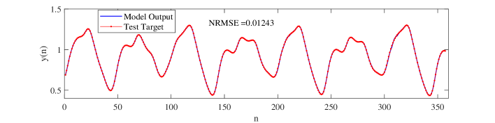
(a) MG

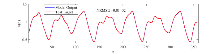
(b) MG1

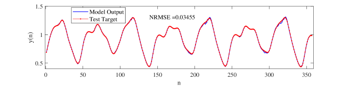
(c) MG2

Figure 2: Prediction fitting curves of the RSCN for MG tasks.

Table 1: Performance comparison of different models on MG tasks.

Datasets	Models	Reservoir size ($N$)	Training time	Training NRMSE	Testing NRMSE
MG	LSTM	6	6.23161±1.44186	0.03270±0.00485	0.03896±0.00379
	ESN	98	0.14388±0.03782	0.01151±0.00216	0.02606±0.00837
	SCR	79	0.13085±0.06283	0.00701±0.00049	0.01538±0.00763
	PESN	83	0.58094±0.18571	0.00582±0.00073	0.01811±0.01029
	LIESN	102	0.41375±0.10283	0.00516±0.00018	0.01374±0.00516
	RSCN	67	0.95787±0.20713	0.00341±0.00037	0.01211±0.00572
MG1	LSTM	7	6.14221±1.17424	0.03119±0.00804	0.03757±0.00771
	ESN	124	0.16983±0.05084	0.01572±0.00679	0.03983±0.01130
	SCR	103	0.13054±0.08291	0.00905±0.00073	0.03550±0.00920
	PESN	109	0.49868±0.10932	0.00881±0.00029	0.03037±0.00525
	LIESN	121	0.66995±0.20232	0.00783±0.00036	0.02559±0.00834
	RSCN	79	0.88928±0.57240	0.00511±0.00032	0.01467±0.00353
MG2	LSTM	5	6.00682±1.10651	0.03586±0.00451	0.08892±0.02503
	ESN	135	0.15339±0.07362	0.03091±0.01927	0.08309±0.01122
	SCR	111	0.12683±0.04328	0.02136±0.00988	0.07661±0.00282
	PESN	113	0.63029±0.14296	0.02493±0.00932	0.08222±0.00631
	LIESN	126	0.45970±0.08371	0.01608±0.00636	0.06525±0.00293
	RSCN	105	1.19886±0.28293	0.00719±0.00589	0.03431±0.00278

Figure 2 illustrates the prediction results of RSCN on three MG tasks, where RSCN exhibits superior performance on the MG task compared to MG1 and MG2, indicating that each input variable contributes to the model output. To comprehensively compare the performance of different models in MG time-series prediction tasks, we summarize the results in Table 1. From Table 1, it can be seen that the NRMSE of each model (excluding LSTM) for MG, MG1, and MG2 increases progressively, suggesting a significant influence of order uncertainty on model performance. The training and testing NRMSE of RSCN are notably lower than other methods. Specifically, compared with the original ESN, the training and testing NRMSE of RSCN are significantly reduced by more than 50% while using fewer reservoir nodes. These results validate the effectiveness of the proposed RSCNs in constructing a concise reservoir with strong learning capabilities for MG time-series prediction. It is worth noting that LSTM exhibits the longest training time, highlighting the potential of randomized learning algorithms in developing efficient models with reduced computational costs. The training time of RSCN is extended as it involves identifying nodes that meet inequality constraints during incremental construction, resulting in higher time consumption.

Figure 3 depicts the errors between the output weights updated by the projection algorithm and the weights trained offline for MG tasks. The gradual reduction in error demonstrates the convergence of the output weights, indicating the stability of the built model.

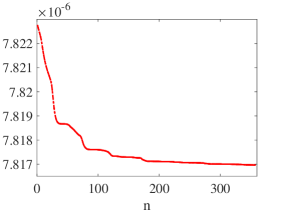
(a) MG

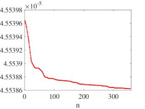
(b) MG1

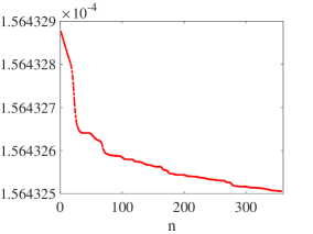
(c) MG2

Figure 3: Errors between the output weights updated by the projection algorithm and the weights trained offline on the three MG tasks.

4.3 Lorenz time-series forecasting

Lorenz chaotic time-series is given by

$$\left\{{\begin{array}[]{*{20}{l}}{\frac{{dx}}{{dn}}{\rm{=}}{a_{1}}\left({y-x}\right)}\\ {\frac{{dy}}{{dn}}{\rm{=}}-xz+{a_{2}}x-y.}\\ {\frac{{dz}}{{dn}}{\rm{=}}xy-{a_{3}}z}\end{array}}\right.$$ (57)

When ${{a}_{1}}=10,{{a}_{2}}=28,{{a}_{3}}=8/3$, and ${{a}_{3}}=8/3$, the Lorenz system exhibits chaotic characteristics. $x\left(n\right)$, $y\left(n\right)$, and $z\left(n\right)$ are the three-dimensional space variables. The input is $\mathbf{u}\left(n\right)={{\left[y\left(n-2\right),y\left(n-1\right),y\left(n\right)\right]}^{\top}}$ and the output is $y\left(n\text{+}1\right)$. In the simulation, the fourth-order Runge-Kutta method is utilized to generate 5000 samples. The first 2500 samples from 1-2500 steps are selected to train the network, 1000 samples from 2501-3500 steps are selected as validation data, and the remaining 1500 samples from 2501-3500 steps are used for testing. For order uncertainty analysis, we assume that $y\left(n\right)$ is unknown, that is, ${{\mathbf{u}}_{1}}\left(n\right)={{\left[y\left(n-2\right),y\left(n-1\right)\right]}^{\top}}$, as the Lorenz1 task.

The performance comparisons of the Lorenz tasks are presented in Table 2. It is evident that all models exhibit better performance on the Lorenz task compared to the Lorenz1 task, highlighting the significance of order information in enhancing the model’s learning capability. Furthermore, our proposed RSCN outperforms other models in terms of reservoir size, training and testing NRMSE, indicating that RSCN can provide a more compact network while achieving superior performance in both learning and generalization.

Figure 4 illustrates the prediction results of RSCN for Lorenz tasks, demonstrating that the model outputs can accurately track the desired output and RSCN performs slightly better on the Lorenz task than the Lorenz1 task. Figure 5 presents the errors between the output weights updated by the projection algorithm and the weights trained offline for the two Lorenz tasks, suggesting the convergence of the output weights and the stability of the model output for a given input.

Table 2: Performance comparison of different models on Lorenz tasks.

Datasets	Models	Reservoir size ($N$)	Training time	Training NRMSE	Testing NRMSE
Lorenz	LSTM	13	16.87905±5.11624	2.97821×10-4±9.93821×10-5	0.00283±0.00107
	ESN	137	0.12775±0.06822	2.72096×10-4±8.29315×10-5	0.00251±0.00098
	SCR	78	0.11309±0.07463	1.07686×10-4±6.98202×10-5	0.00276±0.00037
	PESN	103	1.13184±0.37932	9.92016×10-5±6.30017×10-5	0.00252±0.00021
	LIESN	81	0.64107±0.11282	8.73680×10-5±4.39285×10-5	0.00258±0.00018
	RSCN	66	2.69206±0.39018	5.85655×10-5±2.23991×10-5	0.00213±0.00022
Lorenz1	LSTM	10	12.25693±3.00982	3.67115×10-4±7.36251×10-5	0.00680±0.00155
	ESN	128	0.10230±0.07933	1.60328×10-4±5.28398×10-5	0.00362±0.00128
	SCR	93	0.10822±0.05295	1.95997×10-4±6.18327×10-5	0.00312±0.00067
	PESN	102	1.31079±0.40938	1.46814×10-4±2.39830×10-5	0.00296±0.00034
	LIESN	85	0.54391±0.09363	1.16619×10-4±3.39677×10-5	0.00278±0.00031
	RSCN	81	3.28813±0.23825	8.92229×10-5±2.59028×10-5	0.00237±0.00026

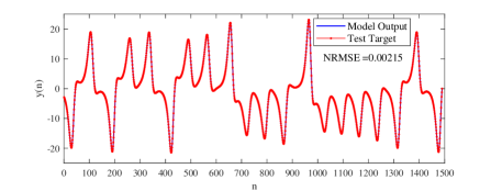
(a) Lorenz

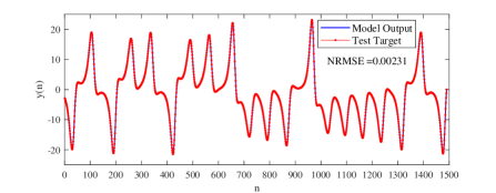
(b) Lorenz1

Figure 4: Prediction fitting curves of the RSCN for Lorenz tasks.

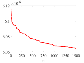
(a) Lorenz

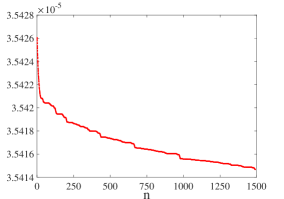
(b) Lorenz1

Figure 5: Errors between the output weights updated by the projection algorithm and the weights trained offline on the Lorenz tasks.

4.4 Nonlinear system identification

In this experiment, two nonlinear system identification tasks are considered. The first dynamic nonlinear plant is as follows

$$y\left({n+1}\right)=0.72y\left(n\right)+0.025y\left({n-1}\right)u\left({n-1}\right)+0.01{u^{2}}\left({n-2}\right)+0.2u\left({n-3}\right).$$ (58)

In the training phase, $u\left(n\right)$ is generated from the uniform distribution $\left[{-1,1}\right]$, and the initial output $y\left(1\right)=y\left(2\right)=y\left(3\right)=0,y\left(4\right)=0.1.$ In the testing phase, the input is

$$u\left(n\right)=\left\{{\begin{array}[]{*{20}{l}}{\sin\left({\frac{{\pi n}}{{25}}}\right),{\kern 1.0pt}{\kern 1.0pt}{\kern 1.0pt}{\kern 1.0pt}{\kern 1.0pt}{\kern 1.0pt}{\kern 1.0pt}{\kern 1.0pt}{\kern 1.0pt}{\kern 1.0pt}{\kern 1.0pt}{\kern 1.0pt}{\kern 1.0pt}{\kern 1.0pt}{\kern 1.0pt}{\kern 1.0pt}{\kern 1.0pt}{\kern 1.0pt}{\kern 1.0pt}{\kern 1.0pt}{\kern 1.0pt}{\kern 1.0pt}{\kern 1.0pt}{\kern 1.0pt}{\kern 1.0pt}{\kern 1.0pt}{\kern 1.0pt}{\kern 1.0pt}{\kern 1.0pt}{\kern 1.0pt}{\kern 1.0pt}{\kern 1.0pt}{\kern 1.0pt}{\kern 1.0pt}{\kern 1.0pt}{\kern 1.0pt}{\kern 1.0pt}{\kern 1.0pt}{\kern 1.0pt}{\kern 1.0pt}{\kern 1.0pt}{\kern 1.0pt}{\kern 1.0pt}{\kern 1.0pt}{\kern 1.0pt}{\kern 1.0pt}{\kern 1.0pt}{\kern 1.0pt}{\kern 1.0pt}{\kern 1.0pt}{\kern 1.0pt}{\kern 1.0pt}{\kern 1.0pt}{\kern 1.0pt}{\kern 1.0pt}{\kern 1.0pt}{\kern 1.0pt}{\kern 1.0pt}{\kern 1.0pt}{\kern 1.0pt}{\kern 1.0pt}{\kern 1.0pt}{\kern 1.0pt}{\kern 1.0pt}{\kern 1.0pt}{\kern 1.0pt}{\kern 1.0pt}{\kern 1.0pt}{\kern 1.0pt}{\kern 1.0pt}{\kern 1.0pt}{\kern 1.0pt}{\kern 1.0pt}{\kern 1.0pt}{\kern 1.0pt}{\kern 1.0pt}{\kern 1.0pt}{\kern 1.0pt}{\kern 1.0pt}{\kern 1.0pt}{\kern 1.0pt}{\kern 1.0pt}{\kern 1.0pt}{\kern 1.0pt}{\kern 1.0pt}{\kern 1.0pt}{\kern 1.0pt}{\kern 1.0pt}{\kern 1.0pt}{\kern 1.0pt}{\kern 1.0pt}{\kern 1.0pt}{\kern 1.0pt}{\kern 1.0pt}{\kern 1.0pt}{\kern 1.0pt}{\kern 1.0pt}{\kern 1.0pt}{\kern 1.0pt}{\kern 1.0pt}{\kern 1.0pt}{\kern 1.0pt}{\kern 1.0pt}{\kern 1.0pt}{\kern 1.0pt}{\kern 1.0pt}{\kern 1.0pt}{\kern 1.0pt}{\kern 1.0pt}{\kern 1.0pt}{\kern 1.0pt}0<n<250}\\ {1,{\kern 1.0pt}{\kern 1.0pt}{\kern 1.0pt}{\kern 1.0pt}{\kern 1.0pt}{\kern 1.0pt}{\kern 1.0pt}{\kern 1.0pt}{\kern 1.0pt}{\kern 1.0pt}{\kern 1.0pt}{\kern 1.0pt}{\kern 1.0pt}{\kern 1.0pt}{\kern 1.0pt}{\kern 1.0pt}{\kern 1.0pt}{\kern 1.0pt}{\kern 1.0pt}{\kern 1.0pt}{\kern 1.0pt}{\kern 1.0pt}{\kern 1.0pt}{\kern 1.0pt}{\kern 1.0pt}{\kern 1.0pt}{\kern 1.0pt}{\kern 1.0pt}{\kern 1.0pt}{\kern 1.0pt}{\kern 1.0pt}{\kern 1.0pt}{\kern 1.0pt}{\kern 1.0pt}{\kern 1.0pt}{\kern 1.0pt}{\kern 1.0pt}{\kern 1.0pt}{\kern 1.0pt}{\kern 1.0pt}{\kern 1.0pt}{\kern 1.0pt}{\kern 1.0pt}{\kern 1.0pt}{\kern 1.0pt}{\kern 1.0pt}{\kern 1.0pt}{\kern 1.0pt}{\kern 1.0pt}{\kern 1.0pt}{\kern 1.0pt}{\kern 1.0pt}{\kern 1.0pt}{\kern 1.0pt}{\kern 1.0pt}{\kern 1.0pt}{\kern 1.0pt}{\kern 1.0pt}{\kern 1.0pt}{\kern 1.0pt}{\kern 1.0pt}{\kern 1.0pt}{\kern 1.0pt}{\kern 1.0pt}{\kern 1.0pt}{\kern 1.0pt}{\kern 1.0pt}{\kern 1.0pt}{\kern 1.0pt}{\kern 1.0pt}{\kern 1.0pt}{\kern 1.0pt}{\kern 1.0pt}{\kern 1.0pt}{\kern 1.0pt}{\kern 1.0pt}{\kern 1.0pt}{\kern 1.0pt}{\kern 1.0pt}{\kern 1.0pt}{\kern 1.0pt}{\kern 1.0pt}{\kern 1.0pt}{\kern 1.0pt}{\kern 1.0pt}{\kern 1.0pt}{\kern 1.0pt}{\kern 1.0pt}{\kern 1.0pt}{\kern 1.0pt}{\kern 1.0pt}{\kern 1.0pt}{\kern 1.0pt}{\kern 1.0pt}{\kern 1.0pt}{\kern 1.0pt}{\kern 1.0pt}{\kern 1.0pt}{\kern 1.0pt}{\kern 1.0pt}{\kern 1.0pt}{\kern 1.0pt}{\kern 1.0pt}{\kern 1.0pt}{\kern 1.0pt}{\kern 1.0pt}{\kern 1.0pt}{\kern 1.0pt}{\kern 1.0pt}{\kern 1.0pt}{\kern 1.0pt}{\kern 1.0pt}{\kern 1.0pt}{\kern 1.0pt}{\kern 1.0pt}{\kern 1.0pt}{\kern 1.0pt}{\kern 1.0pt}{\kern 1.0pt}{\kern 1.0pt}{\kern 1.0pt}{\kern 1.0pt}{\kern 1.0pt}{\kern 1.0pt}{\kern 1.0pt}{\kern 1.0pt}{\kern 1.0pt}{\kern 1.0pt}{\kern 1.0pt}{\kern 1.0pt}{\kern 1.0pt}{\kern 1.0pt}{\kern 1.0pt}{\kern 1.0pt}{\kern 1.0pt}{\kern 1.0pt}{\kern 1.0pt}{\kern 1.0pt}{\kern 1.0pt}{\kern 1.0pt}{\kern 1.0pt}{\kern 1.0pt}250\leq n<500}\\ {-1,{\kern 1.0pt}{\kern 1.0pt}{\kern 1.0pt}{\kern 1.0pt}{\kern 1.0pt}{\kern 1.0pt}{\kern 1.0pt}{\kern 1.0pt}{\kern 1.0pt}{\kern 1.0pt}{\kern 1.0pt}{\kern 1.0pt}{\kern 1.0pt}{\kern 1.0pt}{\kern 1.0pt}{\kern 1.0pt}{\kern 1.0pt}{\kern 1.0pt}{\kern 1.0pt}{\kern 1.0pt}{\kern 1.0pt}{\kern 1.0pt}{\kern 1.0pt}{\kern 1.0pt}{\kern 1.0pt}{\kern 1.0pt}{\kern 1.0pt}{\kern 1.0pt}{\kern 1.0pt}{\kern 1.0pt}{\kern 1.0pt}{\kern 1.0pt}{\kern 1.0pt}{\kern 1.0pt}{\kern 1.0pt}{\kern 1.0pt}{\kern 1.0pt}{\kern 1.0pt}{\kern 1.0pt}{\kern 1.0pt}{\kern 1.0pt}{\kern 1.0pt}{\kern 1.0pt}{\kern 1.0pt}{\kern 1.0pt}{\kern 1.0pt}{\kern 1.0pt}{\kern 1.0pt}{\kern 1.0pt}{\kern 1.0pt}{\kern 1.0pt}{\kern 1.0pt}{\kern 1.0pt}{\kern 1.0pt}{\kern 1.0pt}{\kern 1.0pt}{\kern 1.0pt}{\kern 1.0pt}{\kern 1.0pt}{\kern 1.0pt}{\kern 1.0pt}{\kern 1.0pt}{\kern 1.0pt}{\kern 1.0pt}{\kern 1.0pt}{\kern 1.0pt}{\kern 1.0pt}{\kern 1.0pt}{\kern 1.0pt}{\kern 1.0pt}{\kern 1.0pt}{\kern 1.0pt}{\kern 1.0pt}{\kern 1.0pt}{\kern 1.0pt}{\kern 1.0pt}{\kern 1.0pt}{\kern 1.0pt}{\kern 1.0pt}{\kern 1.0pt}{\kern 1.0pt}{\kern 1.0pt}{\kern 1.0pt}{\kern 1.0pt}{\kern 1.0pt}{\kern 1.0pt}{\kern 1.0pt}{\kern 1.0pt}{\kern 1.0pt}{\kern 1.0pt}{\kern 1.0pt}{\kern 1.0pt}{\kern 1.0pt}{\kern 1.0pt}{\kern 1.0pt}{\kern 1.0pt}{\kern 1.0pt}{\kern 1.0pt}{\kern 1.0pt}{\kern 1.0pt}{\kern 1.0pt}{\kern 1.0pt}{\kern 1.0pt}{\kern 1.0pt}{\kern 1.0pt}{\kern 1.0pt}{\kern 1.0pt}{\kern 1.0pt}{\kern 1.0pt}{\kern 1.0pt}{\kern 1.0pt}{\kern 1.0pt}{\kern 1.0pt}{\kern 1.0pt}{\kern 1.0pt}{\kern 1.0pt}{\kern 1.0pt}{\kern 1.0pt}{\kern 1.0pt}{\kern 1.0pt}{\kern 1.0pt}{\kern 1.0pt}{\kern 1.0pt}{\kern 1.0pt}{\kern 1.0pt}{\kern 1.0pt}{\kern 1.0pt}{\kern 1.0pt}{\kern 1.0pt}{\kern 1.0pt}{\kern 1.0pt}{\kern 1.0pt}{\kern 1.0pt}{\kern 1.0pt}500\leq n<750}\\ \begin{array}[]{l}0.6\cos\left({\frac{{\pi n}}{{10}}}\right)+0.1\cos\left({\frac{{\pi n}}{{32}}}\right)+\\ {\kern 1.0pt}{\kern 1.0pt}{\kern 1.0pt}{\kern 1.0pt}{\kern 1.0pt}{\kern 1.0pt}{\kern 1.0pt}{\kern 1.0pt}{\kern 1.0pt}{\kern 1.0pt}{\kern 1.0pt}{\kern 1.0pt}{\kern 1.0pt}{\kern 1.0pt}{\kern 1.0pt}{\kern 1.0pt}{\kern 1.0pt}{\kern 1.0pt}{\kern 1.0pt}{\kern 1.0pt}{\kern 1.0pt}{\kern 1.0pt}{\kern 1.0pt}{\kern 1.0pt}0.3\sin\left({\frac{{\pi n}}{{25}}}\right),{\kern 1.0pt}{\kern 1.0pt}{\kern 1.0pt}{\kern 1.0pt}{\kern 1.0pt}{\kern 1.0pt}{\kern 1.0pt}{\kern 1.0pt}{\kern 1.0pt}{\kern 1.0pt}{\kern 1.0pt}{\kern 1.0pt}{\kern 1.0pt}{\kern 1.0pt}{\kern 1.0pt}{\kern 1.0pt}{\kern 1.0pt}{\kern 1.0pt}{\kern 1.0pt}{\kern 1.0pt}{\kern 1.0pt}{\kern 1.0pt}{\kern 1.0pt}{\kern 1.0pt}{\kern 1.0pt}{\kern 1.0pt}{\kern 1.0pt}{\kern 1.0pt}{\kern 1.0pt}{\kern 1.0pt}{\kern 1.0pt}{\kern 1.0pt}{\kern 1.0pt}{\kern 1.0pt}{\kern 1.0pt}{\kern 1.0pt}{\kern 1.0pt}{\kern 1.0pt}{\kern 1.0pt}{\kern 1.0pt}{\kern 1.0pt}{\kern 1.0pt}{\kern 1.0pt}{\kern 1.0pt}{\kern 1.0pt}{\kern 1.0pt}{\kern 1.0pt}{\kern 1.0pt}{\kern 1.0pt}{\kern 1.0pt}{\kern 1.0pt}{\kern 1.0pt}{\kern 1.0pt}{\kern 1.0pt}{\kern 1.0pt}{\kern 1.0pt}{\kern 1.0pt}{\kern 1.0pt}{\kern 1.0pt}{\kern 1.0pt}{\kern 1.0pt}{\kern 1.0pt}{\kern 1.0pt}{\kern 1.0pt}{\kern 1.0pt}{\kern 1.0pt}{\kern 1.0pt}{\kern 1.0pt}{\kern 1.0pt}{\kern 1.0pt}750\leq n\leq 1000\end{array}\end{array}}\right..$$ (59)

The output of the nonlinear system is predicted by ${{\left[y\left(n\right),u\left(n\right)\right]}^{\top}}$. The dataset consists of 4000 samples, divided into 2000 for training, 1000 for validation, and 1000 for testing. The initial 100 samples of each set are washed out.

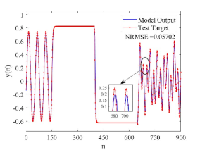
(a) LSTM

(b) ESN

(c) SCR

(d) PESN

(e) LIESN

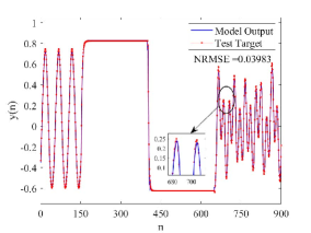
(f) RSCN

Figure 6: The prediction curves of each model for nonlinear system identification I.

The second nonlinear dynamic system can be formulated by

$$y\left({n+1}\right)=\frac{{\left({y\left(n\right)*y\left({n-1}\right)*y\left({n-2}\right)*u\left({n-1}\right)}\right)*\left({y\left({n-2}\right)-1+u\left(n\right)}\right)}}{{1+y\left({n-1}\right)*y\left({n-1}\right)+y\left({n-2}\right)*y\left({n-2}\right)}}.$$ (60)

In the training phase, $u\left(n\right)$ is generated from the uniform distribution $\left[{-0.7,0.7}\right]$, and the initial output are $y\left(1\right)=y\left(2\right)=y\left(3\right)=0$, $y\left(4\right)=0.1.$ In the testing phase, the input is

$$u\left(n\right)=\left\{{\begin{array}[]{*{20}{c}}{0.3*\sin\left({\frac{{\pi n}}{{125}}}\right)+0.2*\sin\left({\frac{{\pi n}}{{25}}}\right){\kern 1.0pt}{\kern 1.0pt}{\kern 1.0pt}{\kern 1.0pt}{\kern 1.0pt}{\kern 1.0pt}{\kern 1.0pt}{\kern 1.0pt}0\leq n<500}\\ {0.6*\sin\left({\frac{{\pi n}}{{25}}}\right){\kern 1.0pt}{\kern 1.0pt}{\kern 1.0pt}{\kern 1.0pt}{\kern 1.0pt}{\kern 1.0pt}{\kern 1.0pt}{\kern 1.0pt}{\kern 1.0pt}{\kern 1.0pt}{\kern 1.0pt}{\kern 1.0pt}{\kern 1.0pt}{\kern 1.0pt}{\kern 1.0pt}{\kern 1.0pt}{\kern 1.0pt}{\kern 1.0pt}{\kern 1.0pt}{\kern 1.0pt}{\kern 1.0pt}{\kern 1.0pt}{\kern 1.0pt}{\kern 1.0pt}{\kern 1.0pt}{\kern 1.0pt}{\kern 1.0pt}{\kern 1.0pt}{\kern 1.0pt}{\kern 1.0pt}{\kern 1.0pt}{\kern 1.0pt}{\kern 1.0pt}{\kern 1.0pt}{\kern 1.0pt}{\kern 1.0pt}{\kern 1.0pt}{\kern 1.0pt}{\kern 1.0pt}{\kern 1.0pt}{\kern 1.0pt}{\kern 1.0pt}{\kern 1.0pt}{\kern 1.0pt}{\kern 1.0pt}{\kern 1.0pt}{\kern 1.0pt}{\kern 1.0pt}{\kern 1.0pt}{\kern 1.0pt}{\kern 1.0pt}{\kern 1.0pt}{\kern 1.0pt}{\kern 1.0pt}{\kern 1.0pt}{\kern 1.0pt}{\kern 1.0pt}{\kern 1.0pt}{\kern 1.0pt}{\kern 1.0pt}{\kern 1.0pt}{\kern 1.0pt}{\kern 1.0pt}{\kern 1.0pt}{\kern 1.0pt}{\kern 1.0pt}{\kern 1.0pt}{\kern 1.0pt}{\kern 1.0pt}{\kern 1.0pt}{\kern 1.0pt}{\kern 1.0pt}{\kern 1.0pt}{\kern 1.0pt}{\kern 1.0pt}500\leq n\leq 800}\end{array}}\right.,$$ (61)

The initial output is set to $y\left(1\right)=-0.3$, $y\left(2\right)=-0.1$, $y\left(3\right)=0.3,$ and $y\left(4\right)=0.$ The output $y\left(n\text{+}1\right)$ is forecasted by ${{\left[y\left(n\right),u\left(n\right)\right]}^{\top}}$. A total of 2000, 1000, and 800 samples are generated as the training, validation, and testing sets, respectively. The first 10 samples of each set are washed out.

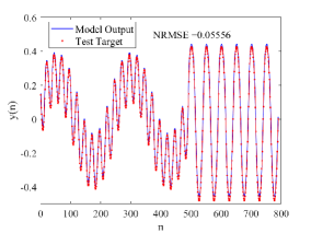
(a) LSTM

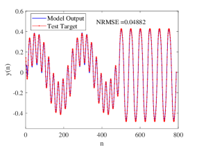
(b) ESN

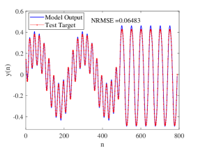
(c) SCR

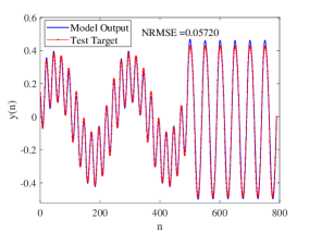
(d) PESN

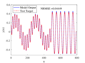
(e) LIESN

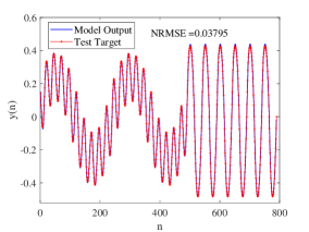
(f) RSCN

Figure 7: The prediction curves of each model for nonlinear system identification II.

Figure 6 and Figure 7 depict the prediction results of each model for the two nonlinear system identification tasks. The model outputs of RSCNs show a closer match with the desired outputs in comparison to other models. These findings demonstrate that RSCNs can quickly adapt to changes in nonlinear dynamic systems, thus confirming the effectiveness of the proposed approach.

To investigate the impact of reservoir size on the model performance, we evaluate the testing performance with different reservoir sizes. Figure 8 illustrates how testing NRMSE varies across reservoir sizes for each method. It is clear that an excessive number of reservoir nodes can result in overfitting. In nonlinear system identification I, overfitting occurs with ESN, SCR, PESN, LIESN, and RSCN when reservoir sizes are 170, 140, 120, 170, and 100, respectively. In nonlinear system identification II, overfitting is less pronounced but still present. Therefore, constructing an effective and concise reservoir topology is crucial for improving tracking performance. RSCN stands out for its ability to generate a suitable network structure by randomly assigning weights and biases through a supervisory mechanism, which also guarantees its universal approximation property.

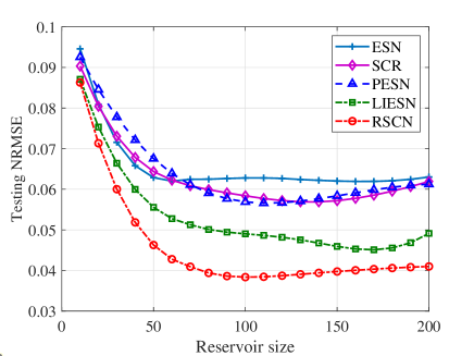
(a) Nonlinear system identification I

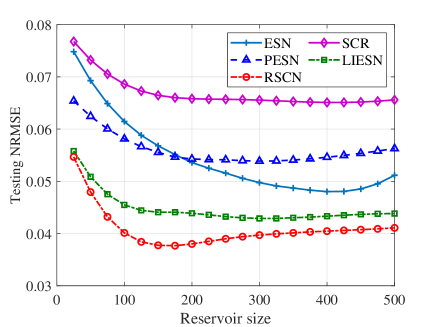
(b) Nonlinear system identification II

Figure 8: Performance comparison of various models with different reservoir sizes on the two nonlinear system identification tasks.

Table 3 presents a comprehensive performance analysis for the two nonlinear system identification tasks. RSCN consistently outperforms LSTM, ESN, SCR, PESN, and LIESN in both training and testing NRMSE. Specifically, for nonlinear system identification I, the training and testing NRMSE obtained by RSCN accounts for 86.68% and 63.07% of those obtained by ESN, while in nonlinear system identification II, they account for 80.21% and 79.01% of ESN results. The superiority of RSCN is further highlighted by its smaller reservoir size compared to other models, which accounts for 64.97% and 35.41% of those obtained by ESN for the two tasks, respectively. This suggests that RSCN can achieve comparable prediction results with fewer nodes, resulting in a more compact reservoir, which is advantageous for temporal data analytics. Additionally, the training time of LSTM is the longest, followed by RSCN, while ESN exhibits the shortest training duration.

The errors between the output weights updated by the projection algorithm and the weights trained offline for the two nonlinear system identification tasks are shown in Figure 9. It is evident that the output weights are converging, indicating that the model is approaching a stable state. This stability is crucial for the precise identification of nonlinear systems, ensuring the model’s reliability and consistency when encountering new data or scenarios.

Table 3: Performance comparison of different models on the two nonlinear system identification tasks.

Datasets	Models	Reservoir size ($N$)	Training time	Training NRMSE	Testing NRMSE
Nonlinear system identification I	LSTM	19	19.28143±6.48212	0.00968±0.01731	0.05556±0.02749
	ESN	157	0.76339±0.01033	0.00916±0.00252	0.06276±0.00325
	SCR	136	0.88387±0.00265	0.00843±0.00064	0.05887±0.00634
	PESN	118	6.08450±0.91907	0.00829±0.00086	0.05848±0.00489
	LIESN	153	1.26218±0.03767	0.00812±0.00051	0.04699±0.00709
	RSCN	102	12.03362±0.85353	0.00794±0.00057	0.03958±0.00097
Nonlinear system identification II	LSTM	15	34.81416±12.31651	0.04276±0.00990	0.05678±0.00654
	ESN	418	1.32246±0.05569	0.03183±0.00225	0.04859±0.00679
	SCR	402	1.33847±0.08379	0.04635±0.00436	0.06498±0.00272
	PESN	325	10.41664±1.07025	0.04155±0.00535	0.05696±0.00236
	LIESN	378	3.55672±0.21922	0.02881±0.00043	0.04481±0.00154
	RSCN	148	14.98757±1.32307	0.02553±0.00593	0.03840±0.00236

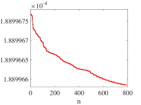
(a) Nonlinear system identification I

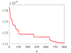
(b) Nonlinear system identification II

Figure 9: Errors between the output weights updated by the projection algorithm and the weights trained offline on the two nonlinear system identification tasks.

4.5 Industrial applications

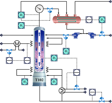
Figure 10: Flowchart of the debutanizer column.

4.5.1 Case 1: soft sensing of butane in dehumanizer column

The debutanizer column plays a crucial role in the desulfurization and naphtha separation unit within petroleum refining production. The flowchart is shown in Figure 10. There are seven auxiliary variables in the refining process, which are described as tower top temperature ${{u}_{1}}$, tower top pressure ${{u}_{2}}$, tower top reflux flow ${{u}_{3}}$, tower top product outflow ${{u}_{4}}$, 6-th tray temperature ${{u}_{5}}$, tower bottom temperature ${{u}_{6}}$, and tower bottom pressure ${{u}_{7}}$. One dominant variable $y$ is the butane concentration at the bottom of the tower, which cannot be directly detected and needs to meet the quality control requirements of minimizing content. This variable is typically obtained through online instrument analysis. The data are generated from a real-time sampling process, with 2394 samples taken at 6-minute intervals. The previous study in [29] has highlighted the delay problem in the debutanizer column, which could be resolved by introducing several well-designed new variables into the original seven variables, that is,

$$\begin{array}[]{l}y\left(n\right)=f\left({{u_{1}}\left(n\right),}\right.{u_{2}}\left(n\right),{u_{3}}\left(n\right),{u_{4}}\left(n\right),{u_{5}}\left(n\right),{u_{5}}\left({n-1}\right),{u_{5}}\left({n-2}\right),{u_{5}}\left({n-3}\right),\left({{u_{1}}\left(n\right)+{u_{2}}\left(n\right)}\right)/2,\\ {\kern 1.0pt}{\kern 1.0pt}{\kern 1.0pt}{\kern 1.0pt}{\kern 1.0pt}{\kern 1.0pt}{\kern 1.0pt}{\kern 1.0pt}{\kern 1.0pt}{\kern 1.0pt}{\kern 1.0pt}{\kern 1.0pt}{\kern 1.0pt}{\kern 1.0pt}{\kern 1.0pt}{\kern 1.0pt}{\kern 1.0pt}{\kern 1.0pt}{\kern 1.0pt}{\kern 1.0pt}{\kern 1.0pt}{\kern 1.0pt}{\kern 1.0pt}{\kern 1.0pt}{\kern 1.0pt}{\kern 1.0pt}{\kern 1.0pt}{\kern 1.0pt}{\kern 1.0pt}{\kern 1.0pt}{\kern 1.0pt}{\kern 1.0pt}{\kern 1.0pt}{\kern 1.0pt}{\kern 1.0pt}{\kern 1.0pt}{\kern 1.0pt}{\kern 1.0pt}{\kern 1.0pt}{\kern 1.0pt}{\kern 1.0pt}{\kern 1.0pt}{\kern 1.0pt}{\kern 1.0pt}{\kern 1.0pt}{\kern 1.0pt}{\kern 1.0pt}\left.{y\left({n-1}\right),y\left({n-2}\right),y\left({n-3}\right),y\left({n-4}\right)}\right).\end{array}$$ (62)

Specifically, considering the order uncertainty, $\left[{{u}_{1}}\left(n\right),\right.$ $\left.{{u}_{2}}\left(n\right),{{u}_{3}}\left(n\right),{{u}_{4}}\left(n\right),{{u}_{5}}\left(n\right),y\left(n-1\right)\right]$ is used to predict the output $y\left(n\right)$. The first 1500 samples are used for training the model, while the next 894 samples are chosen for testing. Gaussian white noise is added to the testing set to generate the validation set. The first 100 samples of each set are washed out.

4.5.2 Case 2: short-term power load forecasting

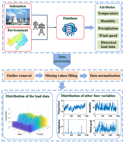
Figure 11: The flowchart of the data collection and processing for the short-term power load forecasting.

Short-term power load forecasting is important for maintaining the safe and stable operation of the power system, enhancing energy efficiency, and minimizing operating costs. The load data used in this work originates from a 500kV substation located in Liaoning, China. Hourly load data was collected from January to February 2023, providing a dataset spanning 59 days. There are four environmental variables including temperature ${{u}_{1}}$, humidity ${{u}_{2}}$, precipitation ${{u}_{3}}$, and wind speed ${{u}_{4}}$ were generated to predict power load $y$. The flowchart of the data collection and processing for the short-term power load forecasting is shown in Figure 11. This dataset consists of 1415 samples, with the first 1000 samples allocated for training and the remaining 415 samples for testing. Gaussian noise is introduced to the testing set to create the validation set. Considering the order uncertainty $\left[{{u}_{1}}\left(n\right),\right.$$\left.{{u}_{2}}\left(n\right),{{u}_{3}}\left(n\right),{{u}_{4}}\left(n\right),y\left(n-1\right)\right]$ is utilized to predict $y\left(n\right)$ in the experiment. The first 30 samples of each set are washed out.

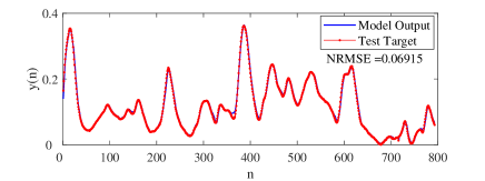
(a) LSTM

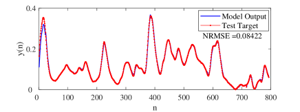
(b) ESN

(c) SCR

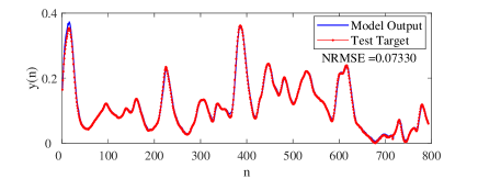
(d) PESN

(e) LIESN

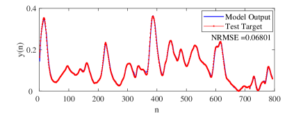
(f) RSCN

Figure 12: The prediction curves of each model for the dehumanizer column process.

Table 4: Performance comparison of different models on the two industry cases.

Datasets	Models	Reservoir size ($N$)	Training time	Training NRMSE	Testing NRMSE
Case 1	LSTM	6	23.02778±5.58473	0.03057±0.00166	0.06937±0.01842
	ESN	213	0.40819±0.12035	0.04085±0.00137	0.08427±0.01144
	SCR	196	0.25422±0.03147	0.03121±0.00098	0.07788±0.01327
	PESN	178	1.54535±0.14082	0.03202±0.00113	0.07572±0.01165
	LIESN	153	0.96202±0.10794	0.02812±0.00123	0.07159±0.01025
	RSCN	87	2.23734±0.20122	0.02734±0.00100	0.06793±0.00411
Case 2	LSTM	5	18.39101±3.26620	0.38257±0.07793	0.75711±0.05489
	ESN	103	0.11881±0.01548	0.24338±0.02189	0.64522±0.07172
	SCR	82	0.08878±0.00927	0.22712±0.01476	0.62350±0.04325
	PESN	156	0.82731±0.03126	0.21028±0.02003	0.60259±0.04522
	LIESN	102	0.61272±0.02190	0.20064±0.02115	0.57546±0.03827
	RSCN	65	0.68257±0.03141	0.19254±0.02047	0.51078±0.03685

Figure 12 and Figure 13 depict the prediction results of different models for the two industry cases, indicating that the output of RSCN aligns more closely with the desired output. Figure 14 illustrates the influence of reservoir size on the testing performance for various models. It can be seen that the testing NRMSE of RSCN consistently outperforms that of the other models. Moreover, the presence of overfitting is observed, with the optimal reservoir sizes for ESN, SCR, PESN, LIESN, and RSCN being 210, 160, 180, 110, and 60 in case 1, and 110, 80, 150, 110, and 70 in case 2.

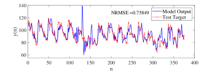
(a) LSTM

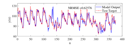
(b) ESN

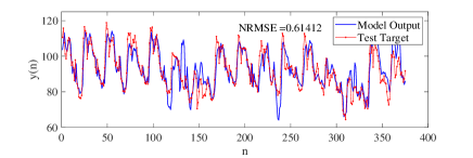
(c) SCR

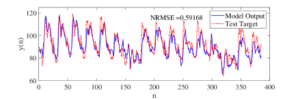
(d) PESN

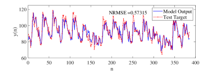
(e) LIESN

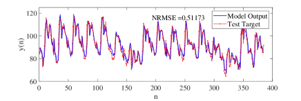
(f) RSCN

Figure 13: The prediction curves of each model for the short-term power load.

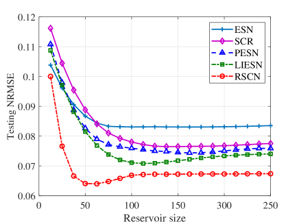
(a) Case 1

(b) Case 2

Figure 14: Performance comparison of various models with different reservoir sizes on the two industry cases.

To comprehensively compare the modelling performance of the proposed RSCN with other classical models, we present the experimental results in Table 4. It can be seen that the training and testing NRMSE of RSCN are lower than other models. In particular, RSCN features a more compact reservoir topology, which can improve computing efficiency and reduce practical application costs. Figure 15 displays the errors in output weights updated by the projection algorithm and the weights trained offline for the two industry cases. The convergence of the output weights is evident, helping to prevent oscillatory or unstable behaviour in the model when applied in practical industrial scenarios. This is important to ensure the smooth operation of systems. These findings validate the effectiveness of the proposed method and highlight its significant potential for modelling complex industrial systems.

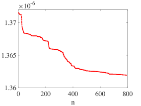
(a) Case 1

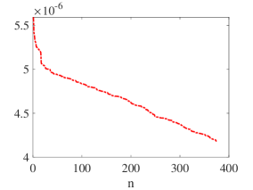
(b) Case 2

Figure 15: Errors between the output weights updated by the projection algorithm and the weights trained offline on the two industry cases.

5 Conclusion

In this paper, a novel randomized learner model termed RSCN is presented for modelling the nonlinear systems with unknown dynamic orders. As an improved version of ESN, RSCN not only maintains the echo state property but also addresses problems such as the sensitivity of random parameter scales and manual structure setting. From the implementation perspective, firstly, the random parameters of the proposed approach are assigned in the light of a supervisory mechanism, and a special structure for the random feedback matrix is constructed. Then, an online update of the output weights is implemented to handle the unknown dynamics. By utilizing this hybrid framework, the universal approximation property of the built model can be ensured for both online and offline learning, and the convergence of learning parameters is guaranteed. The effectiveness of the proposed method is verified on two classical time-series forecasting datasets, two nonlinear system identification tasks, and two industrial cases. The experimental results demonstrate that our proposed RSCNs outperform other models in terms of compact reservoir topology, as well as in learning and generalization performance.

It will be interesting to see more real-world applications of the proposed techniques. Future research could investigate other methods to improve the efficiency of RSCNs, such as alternative supervisory mechanisms or node selection strategies to accelerate error convergence.

References

- [1] Y. Liu, S. Liu, Y. Wang, F. Lombardi, and J. Han. A survey of stochastic computing neural networks for machine learning applications. IEEE Transactions on Neural Networks and Learning Systems, 32(7): 2809-2824, 2021.
- [2] J. Qiu, H. Gao, and S. X. Ding. Recent advances on fuzzy-model-based nonlinear networked control systems: a survey. IEEE Transactions on Industrial Electronics, 63(2): 1207-1217, 2016.
- [3] X. Sun, K. Liu, C. Wen, and W. Wang. Predictive control of nonlinear continuous networked control systems with large time-varying transmission delays and transmission protocols. Automatica, 64: 76–85, 2016.
- [4] J. Wang, H. Wu, and T. Huang. Passivity-based synchronization of a class of complex dynamical networks with time-varying delay. Automatica, 56: 105–112, 2015.
- [5] S. Billings, M. Korenberg, and S. Chen. Identification of nonlinear output-affine systems using an orthogonal least squares algorithm. International Journal of Systems Science, 19(8): 1559–1568, 1988.
- [6] P. Young, A. Jakeman, and R. Mcmurtrie. An instrumental variable method for model order identification. Automatica, 16(3): 281–294, 1980.
- [7] M. Wang, X. Sun, and L. Tao. Bayesian structured variable selection in linear regression models. Computational Statistics, 30(1): 205–229, 2015.
- [8] M. Lucke, X. Mei, A. Stief, M. Chioua, and N. Thornhill. Variable selection for fault detection and identification based on mutual information of alarm series. IFAC-Papers On-line, 52(1): 673–678, 2019.
- [9] G. Hoffmann and C. Tomlin. Mobile sensor network control using mutual information methods and particle filters. IEEE Transactions on Automatic Control, 55(1): 32–47, 2009.
- [10] E. R. Ziegel, G. E. Box, G. M. Jenkins, and G. C. Reinsel. Time series analysis, forecasting, and control. Journal of Time, 31(2): 238–242, 1976.
- [11] I. Leontaritis and S. Billings. Input-output parametric models for nonlinear systems part i: deterministic nonlinear systems. International Journal of Control, 41(2): 303–328, 1985.
- [12] H. Jaeger. The echo state approach to analysing and training recurrent neural networks with an erratum note. Bonn, Germany: German National Research Center for Information Technology GMD Technical Report, 148(34), 2001.
- [13] W. Maass, T. Natschl, and H. Markram. Real-time computing without stable states: a new framework for neural computation based on perturbations. Neural Computing, 14(11): 2531–2560, 2002.
- [14] S. Scardapane and D. Wang. Randomness in neural networks: an overview. Wiley Interdisciplinary Reviews: Data Mining and Knowledge Discovery, 7(2) e1200, 2017.
- [15] M. Li and D. Wang. Insights into randomized algorithms for neural networks: practical issues and common pitfalls. Information Sciences, 382-382: 170–178, 2017.
- [16] D. Wang and M. Li. Stochastic configuration networks: Fundamentals and algorithms. IEEE Transactions on Cybernetics, 47(10): 3466–3479, 2017.
- [17] H. Jaeger, M. Lukoeviius, D. Popovici, and U. Siewert. Optimization and applications of echo state networks with leaky-integrator neurons. Neural Networks, 20(3): 335-352, 2007.
- [18] C. Gallicchio, A. Micheli, and L. Pedrelli. Deep reservoir computing: A critical experimental analysis. Neurocomputing, 268(11): 87-99, 2017.
- [19] X. Wang, Y. Jin, W. Du, and J. Wang. Evolving dual-threshold Bienenstock-cooper-Munro learning rules in echo state networks. IEEE Transactions on Neural Networks and Learning Systems, 35(2): 1572-1583, 2024.
- [20] J. Shi, Y. Leau, K. Li, Y. Park, and Z. Yan. Optimization and decomposition methods in network traffic prediction model: a review and discussion. IEEE Access, 8: 202858-202871, 2020.
- [21] A. Rodan and P. Tino. Minimum complexity echo state network. IEEE Transactions on Neural Networks, 22(1): 131-144, 2010.
- [22] J. Qiao, F. Li, H. Han, and W. Li. Growing echo-state network with multiple subreservoirs, IEEE Transactions on Neural Networks and Learning Systems, 28(2): 391-404, 2016.
- [23] C. Yang, J. Qiao, H. Han, and L. Wang. Design of polynomial echo state networks for time series prediction. Neurocomputing, 290: 148-160, 2018.
- [24] H. Jaeger and H. Haas. Harnessing nonlinearity: predicting chaotic systems and saving energy in wireless communication. Science, 304(5667): 78-80, 2004.
- [25] D. Wang and C. Cui. Stochastic configuration networks ensemble with heterogeneous features for large-scale data analytics. Information Sciences, 417: 55-71, 2017.
- [26] D. Wang and M. Li. Robust stochastic configuration networks with kernel density estimation for uncertain data regression. Information Sciences, 412: 210-222, 2017.
- [27] Y. Wang, M. Wang, D. Wang, and Y. Chang. Stochastic configuration network based cascade generalized predictive control of main steam temperature in power plants. Information Sciences, 587: 123-141, 2022.
- [28] G. Goodwin and K. Sin. Adaptive filtering prediction and control. Courier Corporation, 2014.
- [29] L. Fortuna, S. Graziani, and M. G. Xibilia. Soft sensors for product quality monitoring in debutanizer distillation columns. Control Engineering Practice, 13(4): 499-508, 2005.