Generative Data Assimilation of Sparse Weather Station Observations at Kilometer Scales

Abstract

Data assimilation of observational data into full atmospheric states is essential for weather forecast model initialization. Recently, methods for deep generative data assimilation have been proposed which allow for using new input data without retraining the model. They could also dramatically accelerate the costly data assimilation process used in operational regional weather models. Here, in a central US testbed, we demonstrate the viability of score-based data assimilation in the context of realistically complex km-scale weather. We train an unconditional diffusion model to generate snapshots of a state-of-the-art km-scale analysis product, the High Resolution Rapid Refresh. Then, using score-based data assimilation to incorporate sparse weather station data, the model produces maps of precipitation and surface winds. The generated fields display physically plausible structures, such as gust fronts, and sensitivity tests confirm learnt physics through multivariate relationships. Preliminary skill analysis shows the approach already outperforms a naive baseline of the High-Resolution Rapid Refresh system itself. By incorporating observations from 40 weather stations, 10% lower RMSEs on left-out stations are attained. Despite some lingering imperfections such as insufficiently disperse ensemble DA estimates, we find the results overall an encouraging proof of concept, and the first at km-scale. It is a ripe time to explore extensions that combine increasingly ambitious regional state generators with an increasing set of in situ, ground-based, and satellite remote sensing data streams.

Journal of Advances in Modeling Earth Systems (JAMES)

NVIDIA, Santa Clara, CA, USA University of Oxford, Oxford, UK University of California Irvine, Irvine, CA, USA

Peter Manshausenpeter.manshausen@physics.ox.ac.uk

We demonstrate data assimilation of weather station data to 3km-resolution surface fields with a diffusion model surrogate.

This opens up a simple, scalable pipeline to create km-scale ensemble reanalyses at low cost and latency, competitive to operational ones.

The model is easily adapted to new observations, produces states of variables not directly observed, and shows evidence of learned physics.

Plain Language Summary

Weather forecasts rely on our knowledge of the full state of the atmosphere in the present. Weather stations provide measurements at some (sparse) locations.The atmospheric variables need to be filled in with models that transform the point measurements to a full state (a map). Usually, such models are numerical weather models encoding the physical laws of the atmosphere. They are expensive and slow to run, limiting real-time updates to forecasts. However, recently the machine learning community has presented great advances in similar tasks like filling in missing parts of photographs, and even generating entire videos from a few words. This motivates our use of an ML model trained on km-scale weather data and guided by sparse point measurements to fill in wind and rain maps on the same scale (3km) as state-of-the-art conventional models.

1 Introduction

Machine Learning (ML) has attracted intense interest in the field of global weather forecasting, with models trained off reanalysis outperforming state-of-the-art numerical models [keisler2022forecasting, pathak2022fourcastnet, bi2022pangu, lam2022graphcast]. More recent developments include skillful ensemble forecasting [price2023gencast] and the integration of a numerical dynamical core with online ML parameterizations in one global circulation model [kochkov2023neural]. In order to forecast weather at km-scale, mardani2023residual propose downscaling coarse resolution forecasts with diffusion models [karras2022elucidating]. Together, these advances can be viewed as a disruption of traditional physics-based weather prediction using data-driven approaches stemming from the image and video computer science research community. Dynamical tests suggest that ML video generation is a valid analogy for weather prediction [hakim2024dynamical].

It is natural to wonder if similar transdisciplinary disruptions will modify how the weather and climate communities approach the separate task of state estimation. Forecast initialization and many other applications such as nowcasting depend on high-resolution data assimilation: combining the latest (sparse) observations with our knowledge of the physical laws governing the atmosphere. This inverse problem of estimating a full, dense atmospheric state from observations is traditionally done by constraining numerical models with the available observations. Methods for this include Kalman filters [anderson2001ensemble] and variational methods, see bannister2017review for a review. Similar inverse problems, like inpainting gaps in photographs, and imagining entirely new parts of images, have been successfully addressed with diffusion models [rombach2022highresolution, lugmayr2022repaint].

Data assimilation systems for the regional problem are quite complicated. For example, a premier US regional model—the high resolution rapid refresh (HRRR)[dowell2022high]—depends on outputs of two other data assimilation systems, the Global Forecast System (GFS) and the Rapid Refresh (RAP) [Benjamin2016-ma]. Not all fields and observations are treated consistently, as the dynamical fields (winds, pressure) use classic ensemble methods, while the radar is turned into a latent heating which directly updates the model’s thermodynamics. A separate digital filter is required to avoid high-frequency spin-up artifacts when the observations clash with the model’s fast processes by e.g. violating its notion of hydrostatic balance or saturation [Lynch2003-ju]. Thus, there is an opportunity to simplify and improve the accuracy of these complex pipelines by training cheap ML emulators which admit a simpler formulation of data assimilation algorithms.

Several recent studies already suggest the potential of training a diffusion model emulator of a numerical model– rozet2023scorebased propose Score-based Data Assimilation (SDA), where a similar approach is used to reconstruct states of dynamical systems from observations, experimenting on systems as complex as the two-layer quasigeostrophic equations [rozet2023scorebasedqg]. This framework has been used in the global weather context, assimilating weather stations and satellite data for 2m temperature [qu2024deep]. In related work, huang2024diffda assimilate pseudo-observations of reanalysis data in an autoregressive manner similar to operational data assimilation. These approaches, in contrast to direct forecasting from observations [andrychowicz2023deep], do not include observations in the training of ML models, and hence can be used flexibly to assimilate new observational data streams.

Open questions remain about the performance and calibration of these approaches, and about whether models encode physical relationships. Furthermore, for many impact variables like storms and precipitation, km-scale resolutions are useful. Here, we apply the SDA framework to 3km resolution data of wind and precipitation in the central US. We train a diffusion model with analysis data, and show assimilation of weather station data of the same variables. Section 2 presents the diffusion model and the SDA framework, section 3 discusses the weather station and analysis data used, section 4 shows the assimilation of data in different settings, and section 5 discusses the results.

2 Materials and Methods

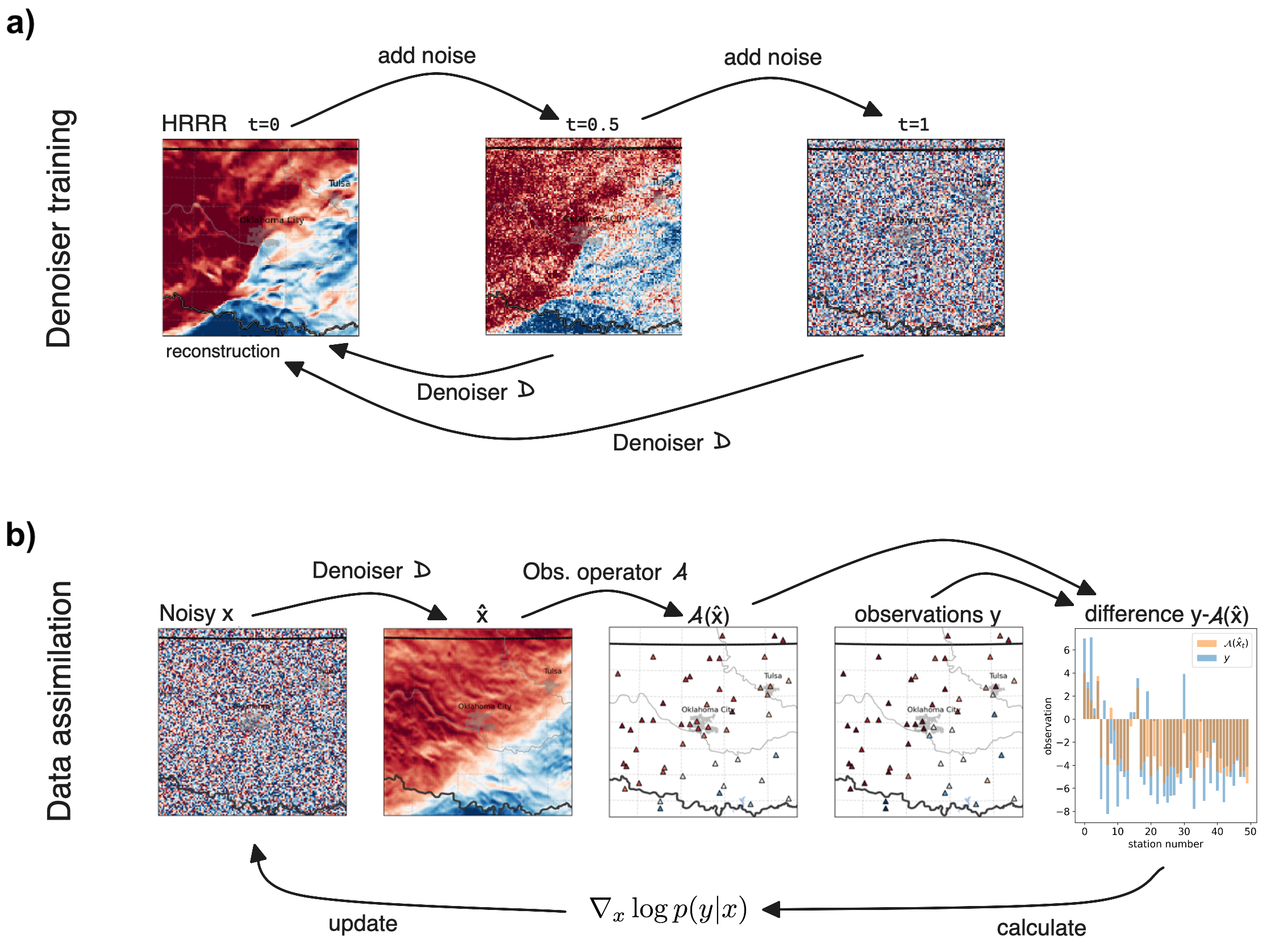
Figure 1: Denoiser training and data assimilation with SDA. a) During the training of the denoiser, noise is added to the training data at different levels, parameterized by time $t\in[0,1]$. The training objective for the denoiser $D$ is to reconstruct the training data, given the noisy state and the time $t$. b) Data assimilation then uses $D$ to go from a noisy state $x$ to a possible denoised state $\hat{x}$. The observation operator $\mathcal{A}$ then maps $\hat{x}$ to the observations it would give rise to, which we compare to the actual observations $y$ (e.g. weather station data). The difference of the two is used to calculate the score $\nabla_{x}\log p(y|x)$, giving the direction in which the noisy state $x$ is updated. This cycle repeats for a number of steps, with time running from 1 to 0, until $x$ is denoised, taking into account the observations and the model’s learned prior (the HRRR reanalysis).

2.1 Diffusion Model for Generation of Kilometer-scale Weather

We train a diffusion model using the Elucidated Diffusion Models (EDM) framework of karras2022elucidating, which was also used in the CorrDiff downscaling model of mardani2023residual. Unlike CorrDiff, we do not condition the model on large-scale meteorology, but train an unconditional diffusion model which generates plausible snapshots of atmospheric states (no forecasting or time dimension). The model is trained to nearly 2.5M images. Figure 1a) shows the objective the model is trained with: Given a sample from the training data with noise added at a certain amplitude, the model is trained to reconstruct the original sample—a process called denoising.

2.2 Score-based Data Assimilation

We adopt the framework of Score-based Data Assimilation (SDA) by rozet2023scorebased with only minor adaptations. In the following, we give an high-level overview and refer to the original paper for a more in-depth discussion.

Score-based data assimilation builds on the score-matching formulation of denoising diffusion models [song2019generative]. Briefly, a forward process maps the data—$x(0)$–onto a known noise distribution $x(T)$. In our case, it is simply given by $x(t)=x(0)+t\epsilon$ where $\epsilon$ is Gaussian white noise [karras2022elucidating]. Intuitively, we can always make data look like noise by adding a lot of noise. It turns out—nearly by magic—that this noising process can be reversed if one knows the so-called score-function $\nabla_{x}\log(p(x(t)|y)$, and in practice large neural networks can be trained to approximate the score-function.

The score-based formulation is so useful for data assimilation because it permits an elegant formulation of Bayes rule,

$$\nabla_{x}\log p(x(t)|y)=\nabla_{x}\log p(x(t))+\nabla_{x}\log p(y|x(t))$$ (1)

where $0\leq t<T$ is the “time” of the noising process, not real-world time. The first term—the score function—is given by the learned denoiser $D$: This is the model described in the previous section, which can generate dynamic system states from noise. In our case, these system states are snapshots of atmospheric states which follow the same distribution (“look like”) the training data. The second term is related to the likelihood: unfortunately, $p(y|x(t))$ is only known at $t=0$—recall that $t=0$ corresponds to the data distribution—but rozet2023scorebased assume a Gaussian observation process

$$p(y|x(t))=\mathcal{N}\big{(}y|\mathcal{A}\left(\hat{x}\right),\Sigma_{y}(t)\big{)}$$ (2)

with variance $\Sigma_{y}$, where $\hat{x}=D(x(t);t))$, the denoised state, and $\mathcal{A}$ is the differentiable observation operator, mapping from the state to the observations (in our case, $\mathcal{A}$ just selects the locations where we have observations from the full state). The Gaussian assumption could impact the spread of the resulting samples since it is mode-seeking. It replaces a potentially complex distribution with a Gaussian distribution. In the inference phase, this score is used for the generation of a full state—this is called ‘guidance’ [rombach2022highresolution, mardani2023variational, ho2022classifier]. Figure 1b) shows how the observations are used for guidance in the denoising process. The score being the log-likelihood, equation 2 takes a very similar shape as the Kalman filtering approach, where the difference $y-\mathcal{A}\left(\hat{x}\right)$ is multiplied with a Kalman gain that depends on the covariances of prior and observations, see e.g. [eq. 9]houtekamer2005ensemble.

Crucially, the denoising model $D$ is not trained on the sparse observation data, but on full atmospheric states from analysis alone. Observations are only supplied at inference time, meaning we do not need to retrain the denoiser when we want to incorporate new observations.

Different from the SDA approaches of rozet2023scorebased, we do not use multiple time steps here, corresponding to a Markov blanket of zero in their description. Other hyperparameters remain largely unchanged from their experiments, with an overview given in C. rozet2023scorebased train their model with a slightly different objective from our denoiser, but the two approaches are compatible. A derivation of how to use a denoiser $D$ trained in the EDM framework of karras2022elucidating in the SDA framework is given in  B.

3 Data

For simplicity, we focus on a region roughly the size of a US state. The square region of interest is bounded by 37.197° to 33.738°N, 99.640° to 95.393°W, symmetric around Oklahoma City and covering most of the state of Oklahoma. This region is chosen mainly due to the stochastic nature of convective precipitation here and the density of the observational network, a setting that makes a stochastic method of data assimilation a natural choice.

3.1 High-Resolution Rapid Refresh (HRRR)

The HRRR [dowell2022high] is an hourly-updated, cloud-resolving, convection-allowing atmospheric model. It is an implementation of the Advanced Research version of the Weather Research and Forecasting (WRF-ARW) Model [skamarockdescription] in the contiguous US and Alaska. It runs on a 3km grid, and assimilates 3km radar data. From the full data, we extract 10m-windspeeds in zonal (east-to-west, 10u) and meridional (south-to-north, 10v) directions as well as total precipitation over one hour (tp) and subset to our study region. This spatial subsetting gives patches of $128\times 128$ pixels. We train with data spanning the period from 2018–2021 inclusive, validating on 2022; nonstationaries in the HRRR data were apparent prior to 2018, limiting the training record to this interval.

3.2 NOAA Integrated Surface Database (ISD)

The ISD [noaaisd] is a global, hourly dataset comprising more than 14,000 weather stations. Here, we download wind and precipitation data in our region of interest for the year of 2017 (out of the HRRR training sample). Wind speed and direction are turned into zonal and meridional surface velocity components. The weather station data is not reported at uniform times, so we interpolate in time to full hours. Our region spans 50 weather stations in the ISD, which in turn have data available in around a third (for wind) and a fifth (for precipitation) of times.

For precipitation,

$$\log(P_{i}+10^{-4})|x\sim\mathcal{N}(\log(P_{i}^{\mathrm{HRRR}}+10^{-4}),\Sigma_{P})$$

where $P_{i}^{\mathrm{HRRR}}$ is the precipitation of the nearest HRRR grid point, and $\Sigma_{P}$ is the estimated observation process noise.

For the winds,

$$\mathbf{u}_{i}|x\sim\mathcal{N}(\mathbf{u}_{i}^{\mathrm{HRRR}},\Sigma_{u})$$

with $\mathbf{u}_{i}^{\mathrm{HRRR}}$ the two wind components at the nearest HRRR grid point. For the values of $\Sigma_{P}$ and $\Sigma_{\mathbf{u}}$ used in the experiments, see C.

4 Results

4.1 Data Assimilation of Analysis Data

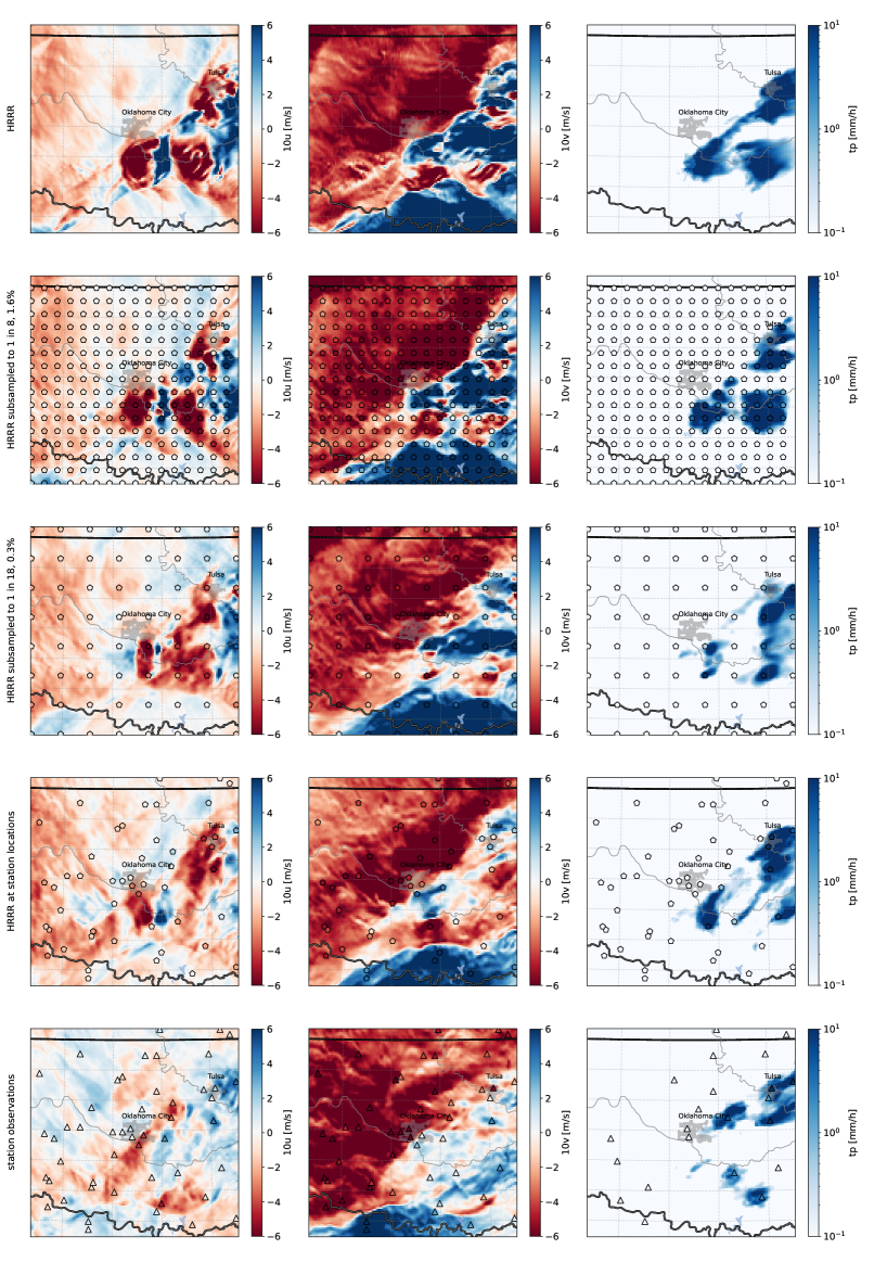
Figure 2: Assimilating increasingly sparse and noisy data. Columns show the different variables 10u, 10v, and tp for different study cases. In row one, we show HRRR data of 2017-05-28 03:00 UTC. Rows two and three show this data subsampled to 1.6% and 0.3%, respectively, in a regular grid (shown as pentagons), plotted over the assimilated high-resolution state. Row four shows the HRRR data subsampled to the locations of our ISD weather stations, as well as the assimilated state. Row five shows the real observations from the stations (triangles), as well as the assimilated state.

We first demonstrate and build confidence in the method’s validity in the limit of realistically sparse weather station data, by assimilating increasingly difficult (pseudo-)observational data to an atmospheric state in Fig. 2. We start with a snapshot of HRRR data in the top row, displaying the two wind variables, and precipitation, which the model is trained for. We first subsample the data to a regular grid of one in eight latitude and longitude positions, resulting in a fraction of $(\frac{1}{8})^{2}=1.6\%$ of the HRRR data. Using these pseudo-observations (pentagons in Fig. 2, second row) in conjunction with our denoiser $D$, we generate an atmospheric state (plotted in the background) which is plausible and very similar to the ground truth full HRRR data (top row). This is similar to the exercise reported by rozet2023scorebasedqg, but for an operational weather model instead of a two-layer quasi-geostrophic model.

To test viability at the sparsity of actual weather station data, we next repeat the experiment on a more extremely subsampled data, to one in 18 or just 0.3% of pixels (Fig. 2, third row). Here, some of the smaller-scale features of the state are not reconstructed accurately, but the larger features are preserved, as should be expected. This still holds when we keep a similar number of pseudo-observations, but choose them in the same irregularly spaced configuration as the weather station data, leaving larger gaps between pseudo-observations (fourth row). We discuss the assimilation of actual observational data in sections 4.3 and 4.4.

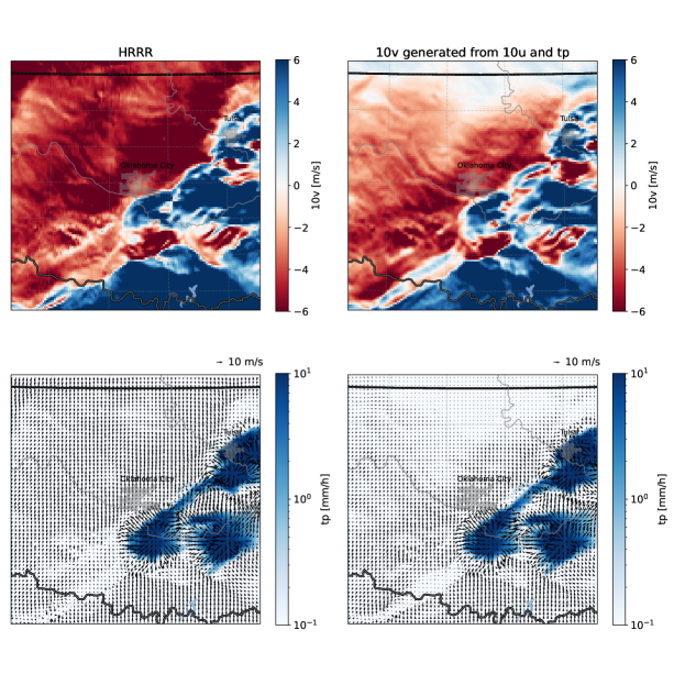
Figure 3: Generating a left-out variable from other variables. We feed the model the HRRR 10u and precipitation, leaving out the 10v channel (top left). The model generates a reasonable 10v (top right). The bottom row shows HRRR tp overlaid with a quiver plot of 10u and 10v from HRRR (bottom left) and 10u and 10v from the model output. Note the wind arrows pointing away from the precipitation in both cases.

4.2 DA of Missing Variables and Learned Physics

To further build confidence, we now test whether the model leverages physically appropriate multivariate relationships in the course of performing state estimation. Despite the fact that the model has been trained with and always outputs the same number of variables – zonal wind, meridional wind, and precipitation rate – we can leave out observations of one of these entirely and obtain a reconstruction purely based on the other variables. We show results of such an experiment in Figure 3: We guide the generation with complete analysis data of the zonal wind and total precipitation variables, leaving out all information about the meridional wind component.

Encouragingly, the model generates a map of the held-out meridional wind that is qualitatively similar to the analysis-truth, in subregions where constraints are apparent. For instance, it succeeds at reconstructing the distinctive gust fronts associated with cold pools [byers1949thunderstorm]: Evaporation of precipitation cooling the air, increasing its density and leading to downdrafts that diverge at the surface. Cold pools feed back on convection [ross2004simple, feng2015mechanisms], and are poorly represented in models, leading to errors in the representation of convection [moncrieff2017simulation]. In our case, where there is precipitation in the analysis data, as well as diverging winds in the u-direction, the model reconstructs diverging winds in the v-direction. Here, the reconstruction agrees very well with the truth. We can hypothesize that even the change in large-scale wind direction from northerly in the northwestern to southerly in the southeastern half of the domain is inferred from the precipitation at the boundary, as this pattern is typical of a weather front. In the northern region of the domain, meridional wind is less constrained by precipitation, possibly causing a larger difference between model prediction and truth. The model associating strong precipitation with diverging near-surface winds provides evidence that it has learned physical behaviour from the training data. Given the importance of terrain for the onset of convection [purdom1976some], we would expect topography to additionally constrain precipitation. We leave an investigation of this effect, as well as a more quantitative study of cold pool dynamics, using e.g. wind gradients [garg2020identifying], for future work.

In sum, we find this qualitative evidence of learnt, physically valid multivariate relationships to add further confidence to the method’s validity. The fact that these relations can be learned and usefully exploited across even within our limited set of three state variables should embolden future attempts that use considerably more ambitious state vectors, within which it is logical to assume additional physical relationships could be exploited in the state estimation.

4.3 Assimilation of Weather Station Observations

Finally, we turn to assimilation of actual weather station data. Guiding the model’s state estimation with the ISD observations provides equally convincing assimilated states as the pseudo-observations. Figure 2 shows one example (bottom row). The weather stations (triangles) are overlaid on the assimilated state. The stochasticity of the generation provides a natural way of producing ensembles of assimilated states, shown in Fig. 4: Even though the observational data and hyperparameters are the same, the state in the second row is different from the last row of Fig. 2, but both agree in the observation locations. This becomes obvious in the standard deviation of the 20-member ensemble plotted in the bottom row of Fig. 4. Standard deviation is small around the locations where the assimilation is guided by observations, and encouragingly large in regions where internal variability from unpredictable dynamics exists - such as for convective precipitation in between station constraints in the east of the domain, and for meridional wind velocity associated with the imperfectly constrained convergence front to the southwest. This also implies that the choice of noise levels $\sigma_{P},\sigma_{u}$ determines the diversity of ensemble states. The mean, in the third row, shows a characteristic blurriness of ensemble means, resulting from averaging the individual members which disagree in small-scale features.

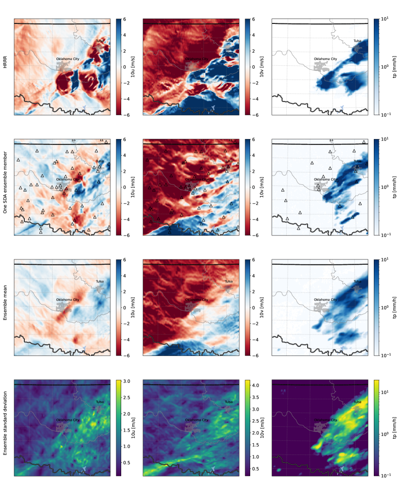
Figure 4: SDA can produce stochastic ensembles of assimilated states. We assimilate the same station data as in Fig. 2, but now generate a 20-member ensemble of states. We show the first member in the second row, the ensemble mean in the third, and the standard deviation in the fourth.

4.4 Performance Evaluation on Left-out Stations

We quantitatively evaluate the model’s performance by comparing the assimilated state, which is obtained by guiding the model inference with a number of observations, with other, left-out observations. First, we test the dependence of SDA performance on the number of stations used for inference, then we fix the number of stations for inference and evaluation and study the performance of ensembles of assimilated states and compare to the HRRR analysis.

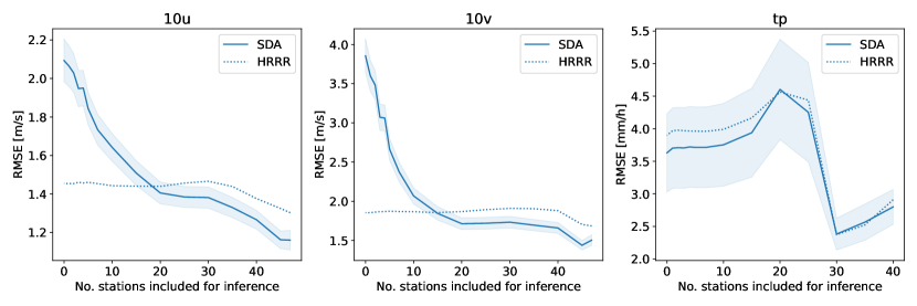
Figure 6: Testing the dependence of assimilation on station density. Evaluating using data from the whole year of 2017, we vary the number of stations used for guiding the inference by the SDA framework. The resulting states are evaluated on the ten held-out stations, giving the RMSEs in each of the variables (solid lines). We also evaluate the RMSE of the HRRR analysis on the same held-out stations (dotted lines).

The results indicate that, even in its crude, low-dimensional, prototype incarnation, SDA already provides more skillful estimates of surface wind than HRRR itself. In Fig. 6, we show how the RMSE of single SDA states decreases, the more station data we use for guiding the inference. We have 50 station locations in the region, so the number of evaluation stations can be found by subtracting inference stations from 50. The HRRR states do not depend on the number of stations used for inference or evaluation, so we expect them to be constant. Departures from a constant HRRR RMSE at large station number for inference can be explained by correspondingly small numbers of evaluation stations (small sample size), and consequently larger stochastic variability, impacting the estimate of RMSE. The intersections of the dotted and solid lines for the wind variables show that around 20 stations are enough for a single SDA assimilation to outperform the HRRR analysis on the held-out stations. The results for precipitation are inconclusive, as the HRRR RMSE is not constant, implying large noise in precipitation RMSE at some stations.

Table 1: Performance metrics of SDA ensembles and the HRRR analysis

	10u [m/s]		10v [m/s]		tp [mm/h]
	SDA	HRRR	SDA	HRRR	SDA	HRRR
RMSE	1.21±0.01	1.44±0.02	1.51±0.02	0.94±0.03	2.06±0.07	2.41±0.07
MAE	0.89±0.01	1.05±0.01	1.13±0.01	1.38±0.01	0.31±0.01	0.39±0.02
CRPS	0.69±0.01	—	0.88±0.01	—	0.29±0.01	—

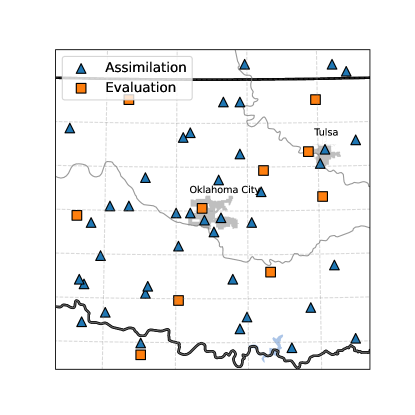
Figure 7: For evaluation we leave out ten randomly selected stations.

Ensemble SDA appears to confirm competitive wind and precipitation state estimates across seasons (see 5. We fix the number of inference stations at 40 and evaluation stations at 10 (for a visualization, see Fig. 7). Moving to ensemble assimilation with 15 members, we show that we outperform HRRR with around 10% lower RMSEs. Full results are given in Table 1. Looking at the time-dependence of the performance, Fig. 5, bottom row, shows that while wind RMSEs are relatively constant in time, precipitation RMSE increases in the summer period, which is characterized by deep convection and heavy rainfall.

It is important to note that HRRR states provide a convenient but not ultimate baseline for km-scale state estimation in this comparison, as the HRRR DA scheme is designed with broader goals than pointwise matching to station data in mind. Nonetheless, HRRR is evaluated partially on its level of mismatch at station data scale, and our main finding is that it is encouraging that a first attempt at km-scale SDA can match or exceed its performance on this metric.

We find ensembles from SDA to be under-dispersive and in need of further calibration for optimal utility. In ensemble forecasting, it is important that the ensemble spread is large where the prediction is uncertain. We also expect this in the assimilation context. In Fig. 5, we show, for each variable, the spread-error diagram and rank histograms. For the spread-error diagram, we compare the ensemble variance (spread) to the MSE of the ensemble mean (error) of all time-samples. A well calibrated ensemble should lie around the dashed 1:1 line. We find that for all variables the spread is smaller than the observed error, meaning that the ensemble is underdispersive [Fortin2014-fc]. Rank histograms show the same effect: For each held-out observation, we determine how it ranks among the 15 ensemble members that are ordered by the predicted value. The u-shaped wind rank histograms show that in many cases, the entire ensemble is either predicting too-large or too-small values. For precipitation, the observations are often larger than the ensemble members, showing a low-bias in SDA precipitation states. We discuss how to improve the calibration in future work in the next section.

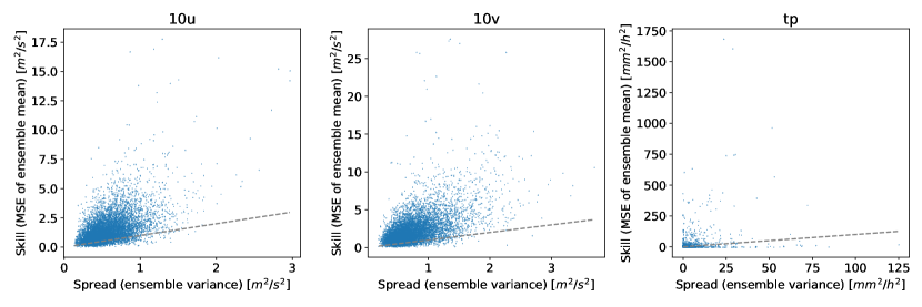
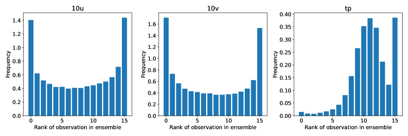
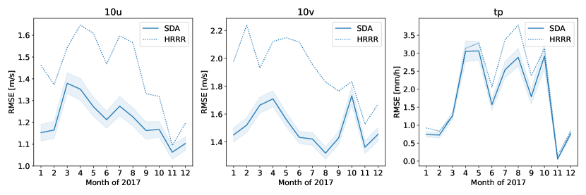
Figure 5: Quantitative evaluation of the SDA assimilation ensemble. The first row shows the spread-skill relationship of the evaluation observations, the second row rank histograms of the 15-member ensemble, the third row the dependence of RMSEs on time of the year.

5 Conclusions

The weather simulation enterprise spans prediction and state estimation. For prediction, machine learning methods from the image and video generation community have already proved disruptive. For state estimation, we have added to evidence that related methods in diffusion ML modeling for inverse problems also have encouraging potential.

In this study, we demonstrate, for the first time, score-based weather station data assimilation at km-scale. We show that - even in a crude, low-dimensional (three-variable) setup - state estimates of surface wind fields outperform the HRRR analysis with respect to held out station observations, with similar errors in precipitation. This is using only a few dozen observations and no remote sensing observations. It is logical to expect extensions of regional SDA that incorporate these may enjoy additional skill gains. We further find evidence of learned physics, which our model can use to reconstruct missing variables. This means that we can effectively constrain unobserved variables in future data assimilation models that produce many more of the variables available in traditional numerical analyses.

A key point is the simplicity of this tooling relative to traditional data assimilation methodology in numerical weather prediction. Crucially, SDA allows for very flexible addition of new observed data, as the observations are only used in the inference phase, not in training, contrasting with the approach of andrychowicz2023deep

While making a convincing case for SDA, we have also shown some limitations of a naive extension of the work of [rozet2023scorebasedqg], on the way to operational use. Firstly, we currently rely only on weather station observations, and only on a subset of the available measurements. We expect other observations like 2m temperature (important e.g. for fronts and cold pools), and pressure (more consistent winds) to improve results. Including satellite, radiosonde, and radar data would further improve assimilation results and allow for more variables, particularly in the vertical direction. However, their incorporation via a more complex observation operator $\mathcal{A}$ may be challenging. Secondly, we show that our SDA ensembles are underdispersive. Calibration has not been previously reported for SDA methods, e.g. by [qu2024deep, huang2024diffda], and we show how it is essential to assess the method’s performance. It is possible some of the error reduction compared to observations could be simple variance reduction. This could be related to mode collapse and low variances produced by our diffusion model. This could be addressed by training the model on more (years or regions of) data, leading to better calibration of the unconditional diffusion (the prior). It could also relate to modal approximation (Eq. 2) used in score-based data assimilation, or our particular choice of hyperparameters (in particular noise parameters $\sigma_{P},\sigma_{u}$), which were tuned for RMSE and CRPS, but not for ensemble dispersiveness.

Future research may also explore making use of the time-dimension of observational data, which would further constrain the atmospheric state. A more flexible approach that could assimilate data at arbitrary times would also improve assimilation, as some error is introduced by first interpolating station data to common points in time.

Appendix A Supplementary Figures

Appendix B Denoiser in the SDA Framework

A diffusion model trained in the EDM framework[karras2022elucidating] $D$ can be translated into the more standard formulation of the SDA framework [rozet2023scorebased] $\epsilon_{\phi}(y,t)$ by using this relationship

$$\epsilon_{\phi}(y,t)=\left(\mu_{t}^{-1}y-D\left(\mu_{t}^{-1}y;\mu_{t}^{-1}\sigma_{t}^{s}\right)\right)\frac{\mu_{t}}{\sigma_{t}^{s}}$$ (3)

To derive this, we first note that the backward ODE in the EDM paper is given by

$$dx=-\dot{\sigma}\sigma\nabla_{x}\log{p\left(\mathbf{x};\sigma\right)}.$$

The forward process is $x(T)=x(0)+\ \sigma(T)\epsilon$. The denoiser is defined by

$$\nabla_{x}\log{p\left(\mathbf{x};\sigma\right)}=\frac{D\left(\mathbf{x};\sigma\right)-\mathbf{x}}{\sigma^{2}}.$$

And trained to minimize the loss given by

$$\left\|D\left(\mathbf{x}+\sigma_{t}\epsilon;\sigma_{t}\right)-\mathbf{x}\right\|^{2},$$

where $\epsilon\sim N(0,I)$.

In SDA, the score function is trained to minimize the loss given by:

$$\sigma_{t}^{2}\left\|s_{\phi}\ \left(\mu_{t}x+\sigma_{t}^{s}\epsilon,t\right)-\epsilon\right\|^{2}\ .$$

where $\epsilon\sim N(0,I)$. For the results, rozet2023scorebased use

$$\mu_{t}=\cos(\omega t),\omega=\cos^{-1}\sqrt{10^{-3}},\sigma_{t}^{s}=\sqrt{1-\mu_{t}^{2}}.$$

Putting the two together yields

$${D\left(\mathbf{x}+\sigma_{t}\epsilon;\sigma_{t}\right)-\mathbf{x-}\sigma_{t}\mathbf{\epsilon+}\sigma_{t}\mathbf{\epsilon}\mathbf{=\ \ }D\left(\mathbf{x}+\sigma_{t}\epsilon;\sigma_{t}\right)-\left(\mathbf{x+}\sigma_{t}\mathbf{\epsilon}\right)\mathbf{+}\sigma_{t}\mathbf{\epsilon}}$$

$${\propto\ -\frac{D\left(\mathbf{x}+\sigma_{t}\epsilon;\sigma_{t}\right)-\left(\mathbf{x+}\sigma_{t}\mathbf{\epsilon}\right)}{\sigma_{t}}\mathbf{-\epsilon}}$$

So therefore,

$$\epsilon_{\phi}\left(\ \mu_{t}x+\sigma_{t}^{s}\epsilon,\ t\right)=\ -\frac{D\left(\mathbf{x}+\sigma_{t}\epsilon;\sigma_{t}\right)-\left(\mathbf{x+}\sigma_{t}\mathbf{\epsilon}\right)}{\sigma_{t}}$$

Then, $y=\mu_{t}x+\sigma_{t}^{s}\epsilon$ so that $x=\mu_{t}^{-1}\left(y-\sigma_{t}^{s}\epsilon\right)$. Substituting this into the argument of $D$ gives

$$x+\sigma_{t}\epsilon=\mu_{t}^{-1}\left(y-\sigma_{t}^{s}\epsilon\right)+\sigma_{t}\epsilon.$$

We cancel the noise terms by setting $\sigma_{t}=\mu_{t}^{-1}\sigma_{t}^{s}$, and finally recover (3).

Appendix C Hyperparameters

We perform minimal hyperparameter tuning on pseudo-observations from HRRR in 2017, in a similar setting as Fig. 2. We find little dependence of RMSEs of our predicted states on number of denoising steps N, corrections C, and correction size $\tau$ above the values reported in the second row of Table 2. Reducing the value of $\Gamma$ to 0.001 from the 0.01 used by rozet2023scorebased was found to improve the results, particularly in the precipitation channel. For the value of $\sqrt{\Sigma_{y}}$, we evaluate the effect of using the values of standard deviations of observations with respect to HRRR data, as a heuristic for the noise of the observation. However we do not find improved skill with channel-wise observed values and therefore keep the original value of 0.1. The values of the second row of Table 2 are used throughout this study, except for section 4.2, where the model diverges in the low-$\Gamma$ setting and we fall back to the original value of 0.01. Additionally we increase the numbers of steps and corrections of the sampling, as for this single sample computational efficiency is less important.

Table 2: Hyperparameters used for experimental results

	N	C	$\tau$	$\sqrt{\Sigma_{y}}$	$\Gamma$
missing channel	256	10	0.3	0.1	0.01
all other results	64	2	0.3	0.1	0.001

Appendix D Open Research

NOAA ISD data [noaaisd] can be obtained freely from the NOAA website, with a useful search functionality under https://www.ncei.noaa.gov/access/search/data-search/global-hourly. HRRR [hrrr] data can be obtained freely from NOAA under https://home.chpc.utah.edu/~u0553130/Brian_Blaylock/cgi-bin/hrrr_download.cgi. Code for the EDM framework [karras2022elucidating] is publicly available under https://github.com/NVlabs/edm, and for SDA [rozet2023scorebased] under https://github.com/francois-rozet/sda. The code used for preprocessing ISD and applying SDA as shown in this paper, as well as the data used for the figures together with figure scripts will be made public upon acceptance of the manuscript.