Rational-Exponent Filters
with Applications to Generalized Auditory Filterbanks

Abstract

We present filters with rational exponents in order to provide a continuum of filter behavior not classically achievable. We discuss their stability, the flexibility they afford, and various representations useful for analysis, design and implementations. We do this for a generalization of second order filters which we refer to as rational-exponent Generalized Auditory Filters/Filterbanks (GAFs) that are useful for a diverse array of applications. We present equivalent representations for rational-order GAFs in the time and frequency domains: transfer functions, impulse responses, and integral expressions - the last of which allows for efficient real-time processing without preprocessing requirements. Rational-exponent filters enable filter characteristics to be on a continuum rather than limiting them to discrete values thereby resulting in greater flexibility in the behavior of these filters. In the case of GAFs, this allows for having arbitrary continuous rather than discrete values for filter characteristics such as (1) the ratio of 3dB quality factor to maximum group delay - particularly important for filterbanks which have simultaneous requirements on frequency selectivity and synchronization; and (2) the ratio of 3dB to 15dB quality factors that dictates the shape of the frequency response magnitude.

I Introduction

I-A Motivation and Goal

Linear time invariant filters are classically represented by rational transfer functions. One generalization of these classical filters is fractional-order filters. Recent interest in fractional-order filters and fractional calculus has increased due to their usefulness for a variety of applications including modeling circuits and systems, control, and filtering signals and noise [1, 2, 3].

Much work on these filters has been dedicated to specific types of fractional-order filters, and especially those that are generalizations of first and second order filters - e.g.,

$$H(s)=\frac{s^{\gamma}}{s^{2\alpha}+2abs^{\alpha}+b^{2}},\quad 0<\alpha<1\;.$$ (1)

These include efforts to analyze the behavior (e.g. stability analysis [4], oscillatory behavior [5], analytic solutions [6]) and develop realizations (e.g. state space formulations based on approximations, fractional-order circuit elements) [7, 8].

We are interested in a different generalization of classical filters that we refer to as rational-exponent filters, and that we represent as a base rational transfer function raised to a rational exponent $B_{u}$,

$$H(s)=H_{base}^{B_{u}}(s)\quad B_{u},\in\mathbb{Q}^{+}\;.$$ (2)

The exponent $B_{u}$ introduces an additional degree of freedom compared to the base filter $H_{base}(s)$. Further allowing $B_{u}$ to be rational and not limiting it to integer values allows for greater flexibility and greater control over the behavior of the filter.

From a theoretical lumped circuit standpoint, non-integer-exponent filters may be thought of as fractional circuits or fractional circuit cascades, in contrast to fractional-order filters that may be represented using fractional circuit elements (e.g. fractional capacitors). Additionally, if a stable system is desired, pole-placement for a rational-exponent filter need only consider the poles of the corresponding base filter, whereas this is a more complicated problem for fractional-order filters. Achieving additional filter design criteria for rational-exponent filters may benefit from those derived for integer-exponent filters [9].

Our goal is to present rational-exponent filters, demonstrate the greater flexibility in filter behavior afforded by these filters compared to their integer counterparts, and derive time and frequency domain representations – that may be useful for realizations as well as further analysis of the filters. We do this for a specific example of rational-exponent filters (which we introduce in the next section). We note previous efforts that discusses another type of rational-exponent filters in which the base filter is first order [10] .

I-B Fractional-Exponent Generalized Auditory Filters and Filterbanks

In this paper, we study rational-exponent filters that are a generalization of second-order filters and are of the form,

$$H(s)=\frac{1}{(s^{2}+2A_{p}s+A_{p}^{2}+b_{p}^{2})^{B_{u}}},\quad A_{p},b_{p}\in\mathbb{R}^{+},B_{u}\in\mathbb{Q}^{+}\;.$$ (3)

Related filters have previously been introduced for the case of integer exponents ($B_{u}\in\mathbb{Z}^{+}$) – the All-Pole Gammatone Filters and Filterbanks (APGFs) [11], and the Generalized Auditory Filters and Filterbanks (GAFs) [12, 9]. For a subset of parameter values, these filters mimic signal processing by the auditory system. In the case of unitary exponents, these filters are simply second order filters. APGFs and GAFs are similar to one another in form, but use different notation, and derivations - GAFs may be used for a variety of signal processing applications as well as the scientific study of the cochlea due to its derivation. Either notation may be used, but we have chosen to use and extend the GAF notation for reasons discussed in appendix A.

Potential applications for GAFs include: multiplexers [13], designing rainbow sensors, [14], analyzing seismic signals [15], underwater sound classification [16], cochlear implants [17], and hearing aids [18]. Due to the nature of these applications, any discussion of GAFs must include a discussion of filterbank representations.

I-C Objectives and Significance

Our objective is to present fractional-exponent GAFs in order to achieve a continuum of possible filter characteristics and behavior without added complexity in stability and causality analyses. We also derive various time and frequency domain representations for the fractional-exponent GAFs.

We are interested in fractional-$B_{u}$ GAFs as they allow for a greater variety of signal processing behavior that can be accomplished compared to the restrictive integer-$B_{u}$ filters or the even more restrictive classical rational transfer functions. While not the topic of this work, an additional benefit of allowing for non-integer-$B_{u}$ GAFs is the ability to better study cochlear mechanisms underlying function.

We derive the various time and frequency domain representations as a means to best fulfill our objective of deriving realizable fractional-$B_{u}$ GAFs. We note that (1) Some representations have restrictions on filter-exponent whereas this constraint may be reduced in others. (2) Certain representations are best suited for extending the GAFs to nonlinear filters. (3) Yet other representations enable parameterizing the filters in terms of desired sets of time or frequency domain filter characteristics - e.g. rise time, settling time, peak frequency, quality factor, group delay, thereby providing a great deal of control over the filter behavior without the need for optimizing over parameter values or using fixed sets of values as is traditionally the case [19]. (4) Other representations may be particularly appropriate for integrator-based implementations.

Having a variety of representations also enables implementational flexibility which is a desirable feature of filters. The ability to implement GAFs in the most suitable way for a particular application may involve designing computer software, or analog or digital hardware architectures. In translating the non-integer-exponent representations into implementations, we might additionally seek inspiration from previous work on realizations for fractional-order filters or their approximations [20, 7, 8]. The integer-exponent instances of GAFs may benefit from existing implementations for related filters [21, 22, 23, 24].

Importantly, we note that for several of applications, simple direct software implementations are most suitable. The representations we present here for fractional-exponent GAFs may directly be used in software and embedded software solutions. Additional work is necessary for developing analog and digital hardware implementations based on some of the representations we derive for non-integer-$B_{u}$ GAFs.

I-D Filterbank Configuration

As mentioned previously, potential applications for rational-exponent GAFs involves its use as a filterbank rather than as a single filter. In deriving the integer- and non-integer-$B_{u}$ GAFs, we are only concerned with filter representations for spatially independent parallel filterbank configurations. We are not interested in spatially dependent configurations [25] such as the non-spatially causal transmission lines [26] and the spatially causal filterbanks in cascade configurations. The former is a fundamentally different form of signal processing and the latter has pole-zero cancellations for the filter which is generally undesirable for most realizations.

We note that the model is derived in the (continuous) frequency domain, and our time domain representations are in continuous time. Our expressions are a function of independent variables - time, frequency, or Laplace-s, or their normalized counterparts. We abuse notation and take liberties in referring to independent variables as frequency or Laplace domains. As this paper is not primarily concerned with implementations, we do not are not concerned with discretizations and transformations to corresponding digital filters here. However, we note that the time domain representations may directly be transformed into their digital counterparts using standard methods.

I-E Organization

To achieve our objective of developing rational-exponent filters - and specifically those that are generalizations of second order filters (GAFs), we present filter representations in the time and frequency domains. We first introduce the reader to the rationale behind deriving each of the representations in this paper (in section II). We then introduce normalized frequency and normalized time domains in which we derive the representations, and which are useful for instances of GAF filterbanks. We present the transfer function representation (previously derived in detail in [12]) in section III and discuss the stability and causality of the rational-exponent filters. We also illustrate the continuum of behavior accessible due to relieving the integer-$B_{u}$ constraint. We then use the transfer function representation to derive the impulse response representation (section IV) and the ODE representation (section V). Our last representation is in the form of integral expressions (section VI) derived from the ODE representation using differential operator theory and extrapolated to non-integer $B_{u}$. Finally, we test the various representations and assess their equivalence using certain inputs in section VII, and provide our conclusions and future directions in section VIII.

II Representations and Normalizations

II-A Representations

In this section, we present the rationale for presenting each of the representations individually. This is in addition to the important rationales of realizability and of collectively having multiple representations for implementational flexibility. The representations are in continuous time and frequency. The time domain representations can directly be translated into their digital counterparts using standard methods. We note that our derivation of the representations for rational-exponent GAF can be used to guide the derivations for other rational exponent filters as well.

II-A1 Transfer functions

GAFs were derived in the frequency domain based on a physical-phenomenological model of the cochlea operating at low stimulus levels and is tightly linked to frequency domain mechanistic variables of the associated cochlear model that are useful for studying how the cochlea functions [12]. Here we extend our study of the transfer functions to rational exponent GAFs. The transfer function representation is the most useful for studying the causality and stability of rational-$B_{u}$ GAFs. Additionally, it is desirable to study the dependence of frequency domain filter characteristics on the values of model constants - which is achievable using the closed-form transfer function expressions. In filter design, it is desirable to achieve certain criteria based on frequency domain filter characteristics, such as values of peak frequency and bandwidth. These can be achieved using the transfer function representation [9].

II-A2 Impulse response

The impulse response representation is another representation that is commonly studied for the dependence of its behavior on model constants. The impulse response representation is useful for parameterizing the filter based on time-domain (specifically impulse response or step response) characteristics such as tonal frequency, rise time, and settling time. This allows for time-domain characteristics-based filter design. We derive the impulse response for integer and half-integer-$B_{u}$ GAFs. We also provide approximations in terms of the highest order term which is a GTF, and discuss the dependence of the behavior of the impulse response on the model constants. Both the impulse response and transfer function representations are appropriate for model testing and for choosing model constant values for which the GAFs mimic natural signal processing in mammals (which is quite desirable for most applications). This is due to the fact that most experimental measurements are in forms of transfer functions and impulse responses [27, 28]. The impulse response is useful for convolution-based implementations [29].

II-A3 ODEs

We derive an ordinary differential equation representation that can be solved with a given set of initial conditions. The ODE representation allows for direct extensions for nonlinear filters as well as introducing delays. The ODE representation (extrapolated to non-integer-$B_{u}$ cases in form only) also enables us to derive the integral representations. While this representation is presented only for integer-$B_{u}$ GAFs and must be derived for each filter order separately, it is quite appropriate for simple and direct software implementations (and embedded systems) and is direct in the sense that it does not require taking any transforms or zero padding and can be done in real-time. Consequently, the ODE representation may be the most suitable for several of the feature-extraction and classification applications and perceptual studies for which the primary requirement is having an easy, direct, software implementation.

II-A4 Integral Expressions

We derive integral representations for rational-$B_{u}$ GAFs. The integral representations are formulated to assume zero initial conditions. The integral representation is parameterized by the filter order and hence, importantly, does not require constructing a different filter for each choice of filter order. They allow for real-time processing without the need for preprocessing such as zero padding or transforms. These representations may particularly be appropriate for integrator-based implementations.

II-B Normalized Frequency

For frequency domain representations (transfer functions), we may consider filterbanks to be constituted of filters, each with a transfer function $H_{i}(\omega)$. Alternatively, we may assign each filter to a fictitious point in space - corresponding to a location along a fictitious cochlea, with a specified peak (characteristic) frequency. This results in $H(x,\omega)$.

If we may express $H(x,\omega)$, in terms of a single variable, $\beta$, as $H(x,\omega)=\mathcal{H}(\beta(x,\omega))$, we consider the variable, $H$ to be‘scaling symmetric’. The scaling symmetry of the transfer functions results in a constant-Q filterbank and is a good local approximation for filterbanks that mimic signal processing in the cochlea.

Consequently, we define our expressions in the normalized angular frequency domain, $\beta$, rather than in $\omega$,

$$\beta\triangleq\frac{f}{\text{CF}(x)}\;,$$ (4)

where $\text{CF}(x)$ is the characteristic frequency map which takes the form, $\text{CF}(x)=\text{CF}(0)e^{\frac{-x}{l}}$. We define the associated $s$ (for the purely imaginary case), as,

$$s(\beta)=i\beta\;,$$ (5)

and use $\hat{s}$ to denote the Laplace-s where needed.

The input to the filters/filterbanks is denoted using $v_{s}(\omega)$ (the notation we use for the input is that of the stapes velocity due to the mechanistic origins of GAF), and the outputs of each filter (or equivalently, at each location) is denoted using $P(x,\omega)$ (in the mechanistic model, this corresponds to differential pressure across the Organ of Corti).

We define a scaling symmetric transfer function, $\mathbf{P}(s)$ as,

$$\mathbf{P}(s)=\frac{P(x,\omega)}{C(x)v_{st}(\omega)}\;,$$ (6)

and provide the expressions for this transfer function in section III.

II-C Normalized Time

For $C$ independent of $\omega$, our model has explicit time domain representations for the filter variable. Here, we introduce normalized time and other time domain variables.

We use $u(t)$ to denote the time domain counterpart of $v_{st}(\omega)$,

$$v_{st}(\omega)\xleftrightarrow{}u(t)\;,$$ (7)

and $q(x,t)$ (rather than $p$) to denote the time domain pressure (relative to $C$) in response to an input,

$$\frac{P(x,\omega)}{C(x)}\xleftrightarrow{}q(x,t)\;,$$ (8)

As frequency is normalized, we define a scaled version of time,

$$\tilde{t}(t,x)\triangleq 2\pi\text{CF}(x)t\;,$$ (9)

to formulate the time domain representations. For instance, we denote the impulse response of normalized pressure (normalized to $C$) as follows,

$$\frac{P(x,\omega)}{C(x)v_{st}(\omega)} =\mathbf{P}(s)=\mathbf{P}\bigg{(}\frac{\hat{s}}{2\pi\text{CF}(x)}\bigg{)}$$ (10)

$$\mapsto g(x,t) =2\pi\text{CF}(x)h(\tilde{t})=2\pi\text{CF}(x)h(2\pi\text{CF}(x)t)\;,$$

where we have made use of the scaling property of Laplace transforms.

The time domain representations derived in this paper - (a) impulse response, (b) ODE, and (c) integral representations, are in continuous time.

III Transfer Functions

As previously mentioned in section II-B, we may consider each filter, $i$, in the filterbank as corresponding to a location, $x$, along a fictitious cochlea. The parallel filterbank transfer function (TF) representation is equation (11), where we have defined $\beta=\frac{f}{\text{CF}(x)}$ (with $s=i\beta$) refers to as normalized frequency or transformed space ($\text{CF}(x)$ providing the characteristic frequency map).

$$\mathbf{P}(\beta(x,\omega)) \triangleq\frac{P(x,\omega)}{Cv_{st}(\omega)}=\Big{(}(s-p)(s-\bar{p})\Big{)}^{-B_{u}}$$ (11)

$$=\Big{(}\frac{1}{s^{2}+2A_{p}s+A_{p}^{2}+b_{p}^{2}}\Big{)}^{B_{u}}$$

where $\mathbf{P}$ at a particular location is a transfer function. Motivated by potential applications, we are primarily interested in cases where the choice of parameter values result in a bandpass filter. In filterbank terminology, a particular location along the length of the cochlea, $x_{i}$ translates to a particular filter, $i$, in the filterbank, where the peak frequency is $\textrm{CF}(x_{i})$. As we’re not interested in specifying $C$, the expression is scaling symmetric (i.e. may be expressed purely as a function of a single variable $\beta(\omega,x)$ rather than both $\omega$ and $x$) in the case that the constants do not vary as a function of location along the length of the cochlea. In the expression, $p=ib_{p}-A_{p}$ and $\overline{p}=-ib_{p}-A_{p}$. The model constants $A_{p},B_{u},b_{p}$ take on real positive values, and we have shown that they vary slowly along the length of the cochlea [12] (recall that for many of the diverse set of applications in section I, it is desirable for the filters to mimic signal processing by the auditory system). If the filters are sharply tuned, $A_{p}^{2}+b_{p}^{2}\approx b_{p}^{2}$, and if the peak frequency occurs at $\text{CF}(x)$ (i.e. $\beta_{peak}=1$), then $b_{p}\approx 1$. In this case, we may simplify the above expression as $\mathbf{P}=\Big{(}\frac{1}{s^{2}+2A_{p}s+1}\Big{)}^{B_{u}}$ which is parameterized by only two constants - $A_{p},B_{u}$. The filters are of exponent $B_{u}$.

The above representation is for parallel filterbank formulations - which is our interest in this paper, the external stimulus is ‘copied’ and acts as the input to the individualized filters at each location along the length of the cochlea. For any given frequency, $f$, each individualized filter has a different $\beta$ (depending on their characteristic frequency, $\text{CF}(x)$), and hence they result in different outputs to the same input even for the case in which the model constants do not vary along the length of the cochlea.

Clearly, the GAFs are second-order filters raised to a power $B_{u}$. For cases in which $B_{u}$ is an integer, the equation results in a rational transfer function with $B_{u}$ pairs of complex conjugate poles. Under these conditions, the expressions clearly show that the linear model is a infinite impulse response (IIR) system that is stable and realizable.

In the case that $C(\omega)=C\in\mathbb{R}$, then a real input results in a real output even if the exponent, $B_{u}$, is a non-integer number. Rational-exponent filters are stable. We demonstrate BIBO stability by making the following observation: For the case of $B_{u}=\frac{m}{n}$ where $m,n\in\mathbb{Z}^{+}$ and finite, sequential processing by $n$ filters is equivalent to a stable $m^{th}$ order system because the poles are in the left half plane. Consequently, each constitutive filter of order $B_{u}$, where $B_{u}$ is a positive rational number, must be stable. The causality of rational-exponent filters also arises from a similar argument, and is also apparent from the various time-domain representations in the subsequent sections.

While we expect these properties to hold for the more general case of $B_{u}\in\mathbb{R}^{+}$ due to continuity, we are not concerned with this extension. This is because, practically, there is nothing to be gained in terms of finer tuning and wider array of signal processing behavior by moving from rational to real $B_{u}$. Consequently, we do not discuss stability of real-exponent filters.

Our above analysis regarding causality and stability of rational- exponent filters are not restricted to GAFs. Unlike fractional-order filters which require a more involved stability analysis [4], the only condition for the stability and causality of any rational-exponent filter is that the base filter is a rational transfer function that itself is stable and causal. Accordingly, filter design and pole placement for a stable non-integer exponent filter is particularly simple for cases where the base filter is up to fourth order (in which case their are closed form expressions relating filter coefficients and poles).

We next analyze the dependence of the behavior of the GAF TFs on the three model constants, $A_{p},b_{p},B_{u}$:

• The peak normalized frequency is $b_{p}$

• Group delay increases proportionally with $B_{u}$ and inversely with $A_{p}$

• Bandwidth increases proportionally with $A_{p}$ and decreases in a more involved patter with $B_{u}$

Figure 1 shows the Bode plots for various values of $B_{u}$ and illustrates the flexibility in behavior afforded by relieving the integer restriction. Figure 2 quantifies this by demonstrating the continuum of filter characteristics afforded by having rational $B_{u}$. For instance, the plot for the ratio of quality factor to group delay (which is practically purely a function of $B_{u}$ [30]) shows that reducing the integer-$B_{u}$ constraint to a rational one, practically allows for accessing a continuum of this ratio rather than discrete values. Greater flexibility in controlling this ratio is particularly important for filter banks where frequency selectivity and synchronization requirements are important. Similarly, allowing for non-integer values of $B_{u}$ results in a continuum of values for the ratio of the 3dB quality factor to 15dB quality factor which controls the shape of the magnitude of the filter response. These observations demonstrate the fact that non-integer-$B_{u}$ GAFs have a wider set of accessible behaviors than those restricted to integer $B_{u}$.

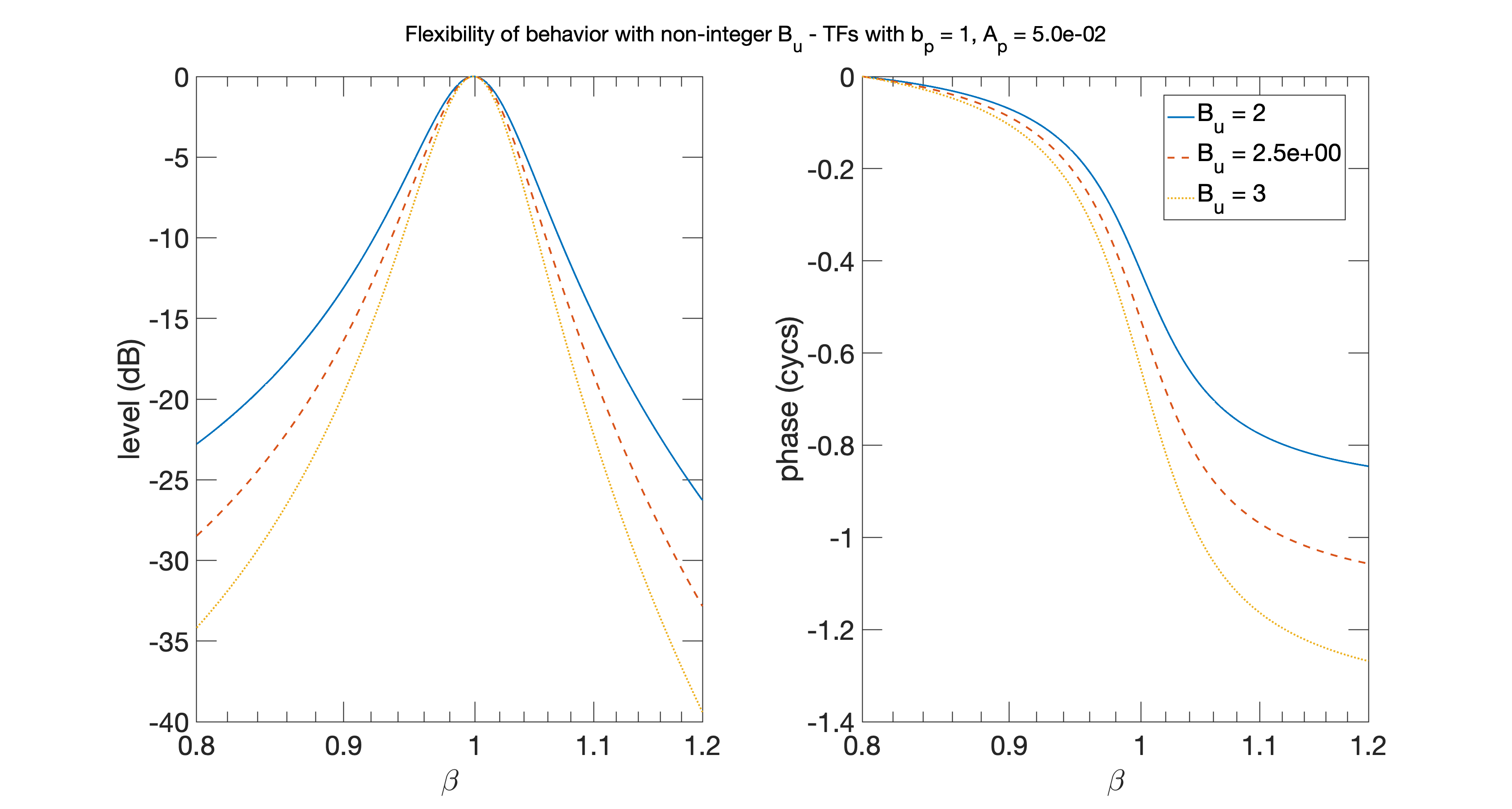
(a) $A_{p}=0.05,B_{u}\in\{2,2.5,3\}$

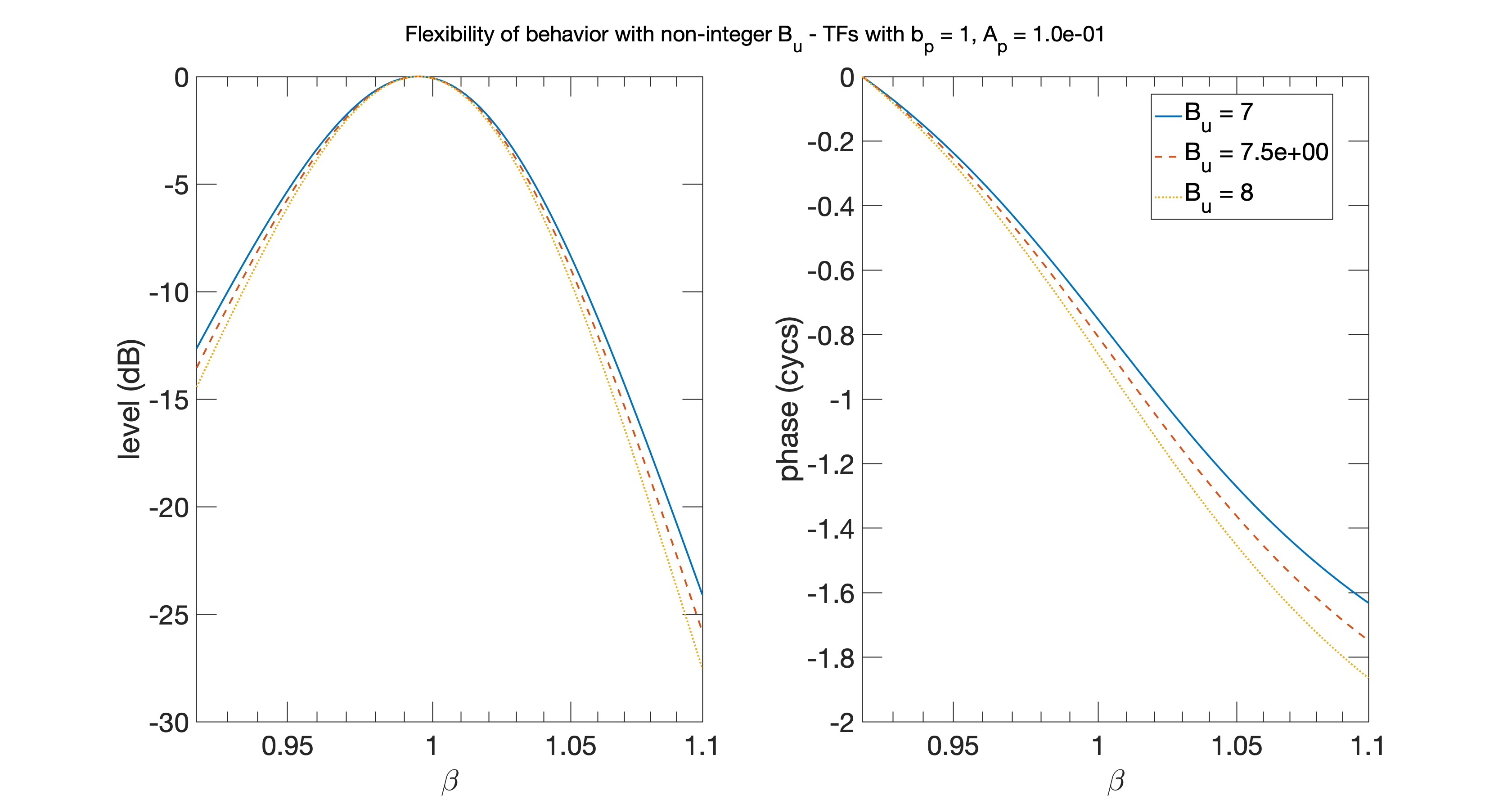
(b) $A_{p}=0.1,B_{u}\in\{7,7.5,8\}$

Figure 1: Allowing for non-integer $B_{u}$ enables greater variety of behavior: Figure shows Bode plots GAFs with integer and half-integer $B_{u}$. The two sets of figures are generated with different values for the model constant $A_{p}$ and different ranges for $B_{u}$. The left set of figures is more sensitive to changes in $B_{u}$ in non-integer increments, illustrating that the flexibility in signal processing behavior afforded by relieving the integer constraint depends on the values of $A_{p}$ and $B_{u}$. In these plots, the magnitude (in dB) is plotted in reference to the magnitude at the peak, and the phase (in cycles) is in reference to the first phase.

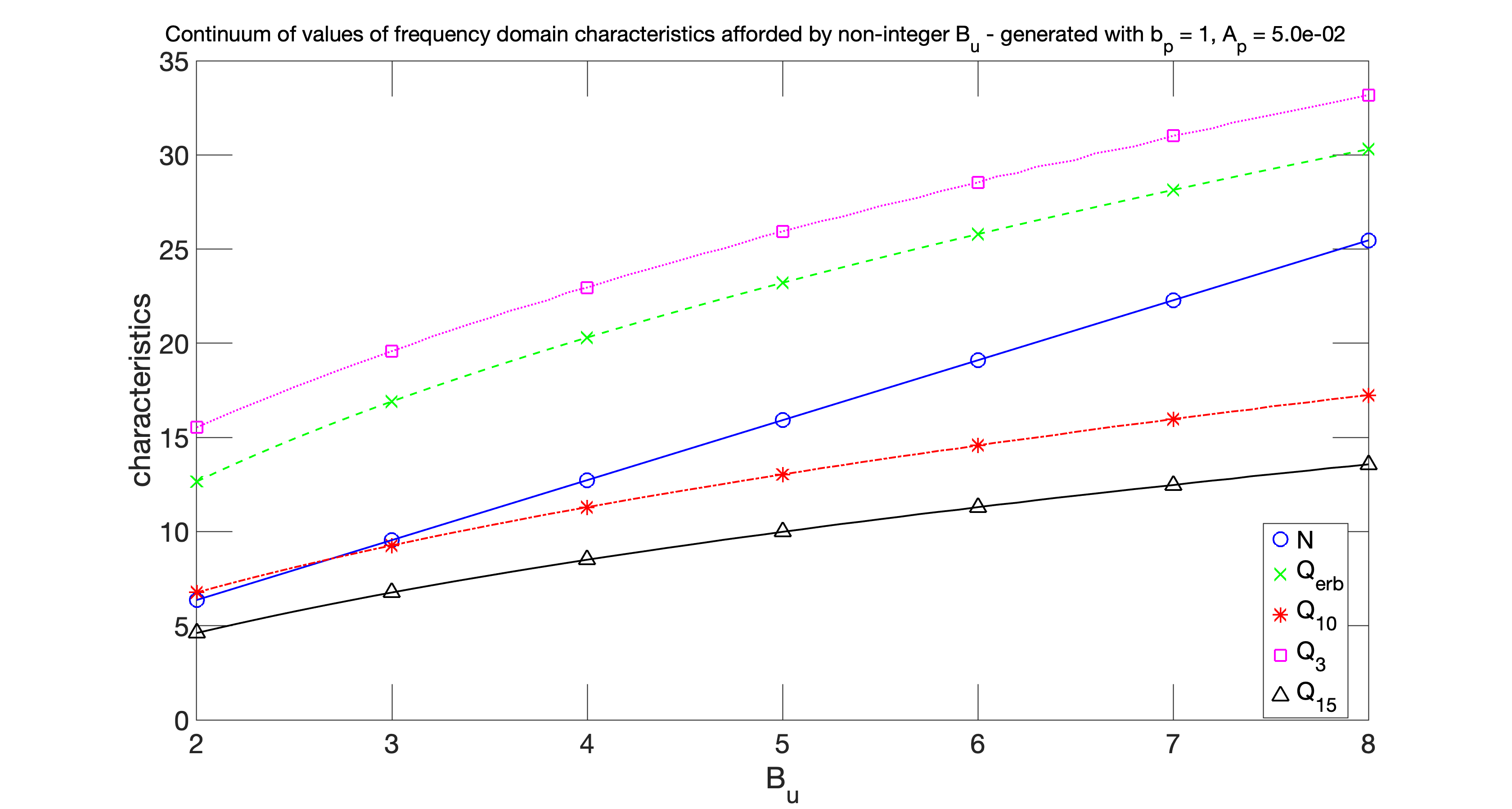
(a) $Q_{erb}$ is the quality factor generated from the equivalent rectangular bandwidth $Q_{erb}=\frac{\beta_{peak}}{\textrm{ERB}_{\beta}}$; $Q_{15},Q_{10},Q_{3}$ are the quality factors computed using 15, 10, and 3 dB bandwidths respectively; and $N$ is a normalized group delay, $N=-\frac{1}{2\pi}\frac{d\textrm{phase}\{\mathbf{P}\}}{d\beta}$

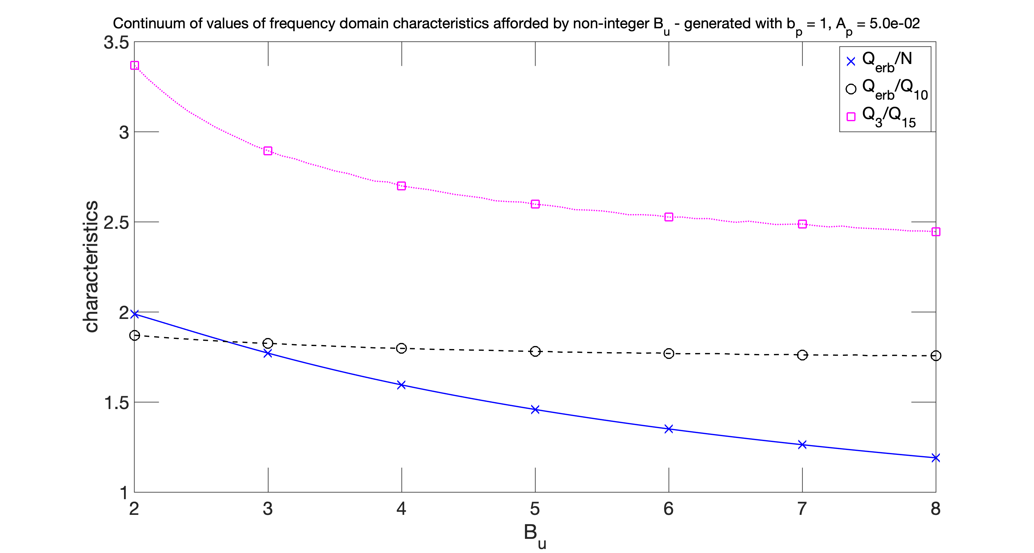
(b) Ratio of quality factor to group delay $\frac{Q_{erb}}{N}$ (which relates frequency selectivity to delay) which shows a great degree of dependence on $B_{u}$, and the ratio of various quality factors to one another.

Figure 2: Allowing for rational, rather than only integer, $B_{u}$ provides greater flexibility in behavior: The figures show the continuum of behavior (quantified by TF characteristics) that may be accessed once we relieve the integer-$B_{u}$ restriction (lines), as opposed to the discrete behavior accessible via the restricted integer-$B_{u}$ cases (shapes). The left figure shows the continuum of behavior as a function of (practically) continuous $B_{u}$ for simple filter characteristics while holding $A_{p}$ constant - to satisfy other criteria on characteristics. The right figure shows the continuum of behavior for compound characteristics that practically only depend on $B_{u}$ (strictly speaking $\frac{Q_{erb}}{N}$ also depends on $b_{p}$ but this is generally fixed to unity so that the peak occurs at the selected $\text{CF}(x)$).

The TF representation is ideal for testing the model against data and for estimating values of model constants from data due to the nature of much of the reported data from cochlear experiments [28]. We have demonstrated these points in previous work [12]. Additionally, the simplicity of the form of the TF representation allows us to derive parameterizations of GAFs in terms of desired or observed filter/response variable characteristics such as peak frequency, quality factor, and group delay [30]. This is quite desirable for an array of signal processing applications as well as for understanding the relationship between observed function and underlying mechanisms in the cochlea.

Architectures for analog and digital hardware may easily be developed based on the TF representation for the case of integer $B_{u}$ - e.g as delay equations in the form, $x[n]=\sum\limits_{k=0}^{M}a[k]x[n-k]-by[n]$ due to the all-pole nature of $\mathbf{P}$. We may especially leverage existing work on implementations of the APGF. In figure 3, we demonstrate the ability to process signals using TFs with non-integer-$B_{u}$ and hence the ability to use it for software implementations. Future work may involve developing analog and digital implementations based on the non-integer-$B_{u}$ TFs (or other representations) which may benefit from approximation and truncation methods and existing work on implementations of fractional-order filters of the classical form.

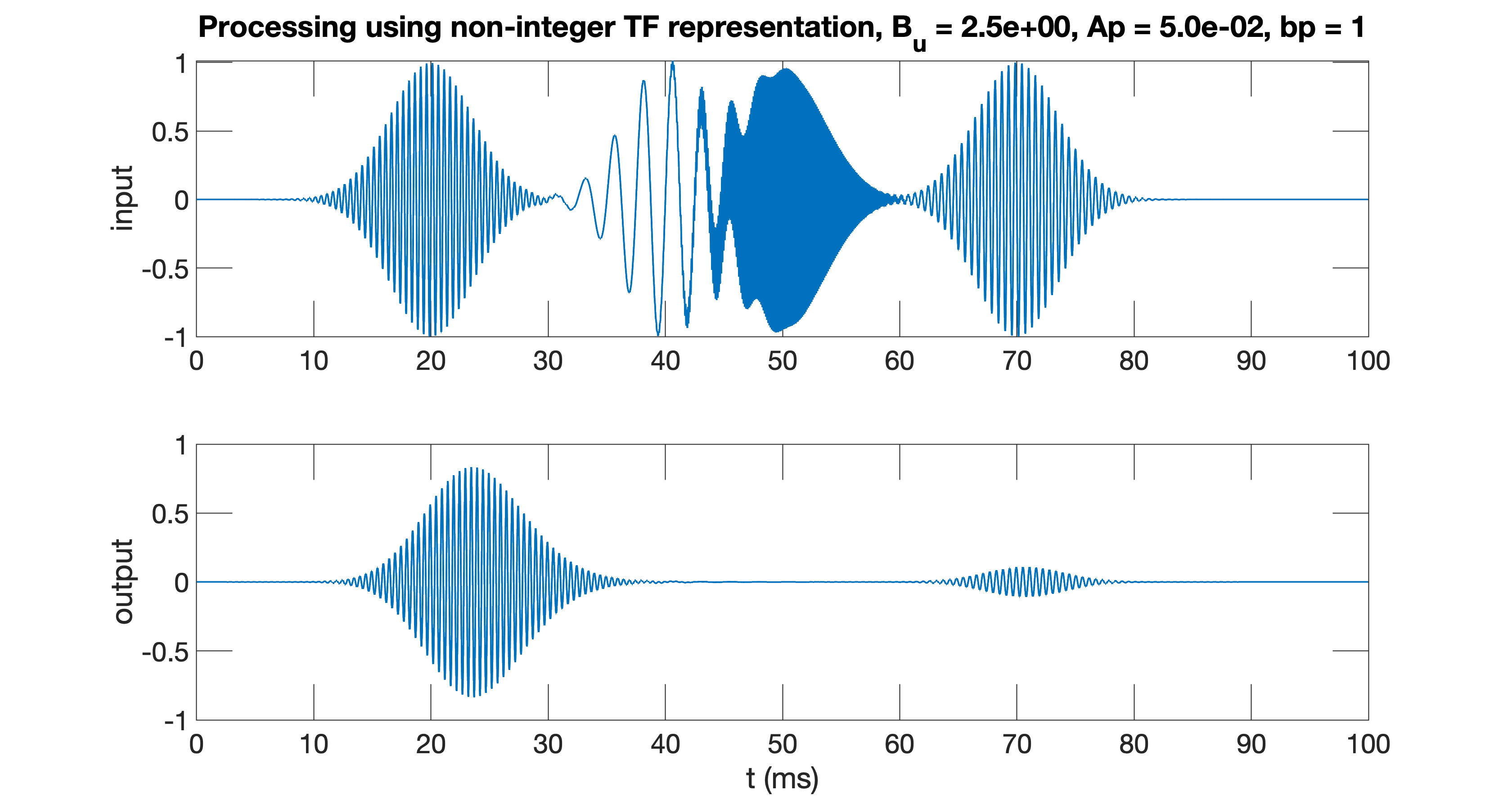
Figure 3: Software implementations of the non-integer-$B_{u}$ TF representation can be used to process signals: The output (bottom panel) of a chosen filter in a filterbank with peak frequency 2 kHz (or equivalently at a chosen location along the length of the cochlea with $\text{CF}(x)=2$ kHz) is computed using a software implementation of the TF representation using a non-integer-$B_{u}$ value of $2.5$. The output is generated in response to a input signal (top panel) a composed of tone pips and is of the form $v_{stapes}=\sum_{i=0}^{3}e^{-(t-t_{i})^{2}/T^{2}}sin(2\pi f_{i}t)$, where $T=5,f_{0}=\textrm{CF},t_{0}=20,f_{1}=5\textrm{CF},t_{1}=50,f_{2}=\frac{7}{8}\textrm{CF},t_{2}=70,f_{3}=\frac{1}{5}\textrm{CF},t_{3}=40$ with frequency in kHz, and time in ms. As expected, the filter responds maximally to frequency components closest to its $\text{CF}(x)$. This figure illustrates realizability of software implementations using the TF representation with non-integer-$B_{u}$.

For implementations beyond that of a single filter (corresponding to processing until a single location), we may simply compute different $s$ for each filter depending on its characteristic frequency. In this way, the model constants are the same across filters and is quite appropriate for software implementations. Alternatively, we may use the equivalent Laplace domain representations of the transfer function of constituent filters in the filterbank. We use $\hat{s}$ for the Laplace-s variable rather than the typical $s$ notation which we have already used. This results in,

$$\frac{P(x,\omega)}{v_{st}(\omega)}=C_{1}(x,\omega)\bigg{(}(\hat{s}-2\pi\text{CF}(x)p)(\hat{s}-2\pi\text{CF}(x)\overline{p})\bigg{)}^{-B_{u}}\;,$$ (12)

where, $C_{1}(x,\omega)=C(x,\omega)\bigg{(}2\pi\text{CF}(x)\bigg{)}^{2B_{u}}$. Setting $C(x,\omega)=C$ results in filters with equal peak magnitudes across filters for the spatially invariant model constant case.

IV Impulse Responses

The $h(\tilde{t})$ of the normalized pressure impulse response, $g=2\pi\text{CF}(x)h(\tilde{t})$ can be expressed as a function of scaled time, $\tilde{t}$, (which also encodes location). We also define, purely for the purposes of compactness,

$$\tilde{t}_{b}\triangleq b_{p}\tilde{t}\;.$$ (13)

Much can be inferred about a system from its impulse response. In this section, we derive expressions for the impulse response and study its features and dependence on model constants. We begin by deriving impulse responses for integer$B_{u}$ GAFs, then do so for half-integer-$B_{u}$ cases. For integer $B_{u}$ we have a restriction of $B_{u}>1$ in order to mimic cochlear signal processing. For half-integer $B_{u}$ this restriction is further refined to $B_{u}\geq\frac{3}{2}$ in order to achieve impulse responses for which the envelope can grow then decay.

IV-A Integer $B_{u}$

Here we derive the $h(\tilde{t})$ of the impulse responses, $g$, for the cases of integer $B_{u}$. We do not discuss $B_{u}=1$ as it does not provide the appropriate envelope structure and instead corresponds to an impulse response with $h(\tilde{t})=\frac{e^{-A_{p}\tilde{t}}\sin(b_{p}\tilde{t})}{b_{p}}$, that will decay without a prior rise which is inconsistent with measurements. In table I, we present $h(\tilde{t})$ for various integer values of $B_{u}$, and plot two such instances in the top panel of figure 4.

$\mathbf{B_{u}}$	$\mathbf{h(\tilde{t})=}$
$2$	$\frac{1}{2b_{p}^{3}}e^{-A_{p}\tilde{t}}\bigg{(}\sin(\tilde{t}_{b})-\tilde{t}_{b}\cos(\tilde{t}_{b})\bigg{)}\xrightarrow[\text{approx.}]{\text{highest-order}}\frac{1}{2b_{p}^{3}}e^{-A_{p}\tilde{t}}\bigg{(}-\tilde{t}_{b}\cos(\tilde{t}_{b})\bigg{)}$
$3$	$\frac{1}{8b_{p}^{5}}e^{-A_{p}\tilde{t}}\bigg{(}3\sin(\tilde{t}_{b})-3\tilde{t}_{b}\cos(\tilde{t}_{b})-\tilde{t}_{b}^{2}\sin(\tilde{t}_{b}))\bigg{)}\xrightarrow[\text{approx.}]{\text{highest-order}}\frac{1}{8b_{p}^{5}}e^{-A_{p}\tilde{t}}\bigg{(}-\tilde{t}_{b}^{2}\sin(\tilde{t}_{b}))\bigg{)}$
$4$	$\frac{1}{48b_{p}^{7}}e^{-A_{p}\tilde{t}}\bigg{(}15\sin(\tilde{t}_{b})-15\tilde{t}_{b}\cos(\tilde{t}_{b})-6\tilde{t}_{b}^{2}\sin(\tilde{t}_{b})+\tilde{t}_{b}^{3}\cos(\tilde{t}_{b}))\bigg{)}\xrightarrow[\text{approx.}]{\text{highest-order}}\frac{1}{48b_{p}^{7}}e^{-A_{p}\tilde{t}}\bigg{(}\tilde{t}_{b}^{3}\cos(\tilde{t}_{b}))\bigg{)}$
$5$	$\frac{1}{384b_{p}^{9}}e^{-A_{p}\tilde{t}}\bigg{(}105\sin(\tilde{t}_{b})-105\tilde{t}_{b}\cos(\tilde{t}_{b})-45\tilde{t}_{b}^{2}\sin(\tilde{t}_{b})+10\tilde{t}_{b}^{3}\cos(\tilde{t}_{b})+\tilde{t}_{b}^{4}\sin(\tilde{t}_{b}))\bigg{)}\xrightarrow[\text{approx.}]{\text{highest-order}}\frac{1}{384b_{p}^{9}}e^{-A_{p}\tilde{t}}\bigg{(}\tilde{t}_{b}^{4}\sin(\tilde{t}_{b}))\bigg{)}$

TABLE I: $h(\tilde{t})$ expressions, including the scaling coefficient, for several cases of positive integer values of $B_{u}$ obtained from the inverse transform of the transfer function. These may also be generated from equation 15. The integer value $B_{u}=1$ is not appropriate as it results in $\frac{e^{-A_{p}\tilde{t}}\sin(\tilde{t}_{b})}{b_{p}}$ in which the envelop only decays contrary to the desired behavior of the cochlea and auditory filters.

In the top panel of figure 4, we have illustrated the impulse response for two different values of the model constant $B_{u}$ which controls the phase of the oscillatory factor. The two illustrated cases have opposite polarity with respect to one another at the same $\tilde{t}_{b}$. In experimentally measured basilar membrane click responses, all the peaks measured from different locations along the cochlea approximately align in the same direction [31]. Therefore, this matching polarity (after accounting for scaled time) may also be used to determine possible $B_{u}$, as well its variation along the length of the cochlea.

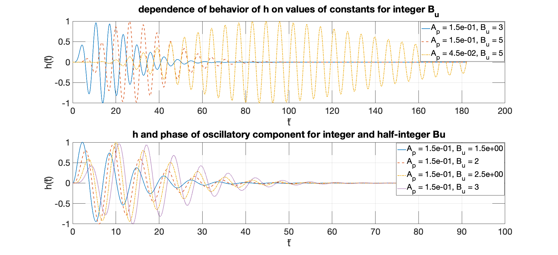
Figure 4: Normalized model impulse responses for pressure as a function of normalized time $\mathbf{\tilde{t}=2\pi\text{CF}(x)t}$ with $\mathbf{b_{p}=1}$. Top: shows the dependence of the impulse response (table I, plotted as normalized to the maximum absolute value) behavior on the model constants. For instance, delay increases with increasing $B_{u}$ and decreasing $A_{p}$. This is generated by varying integer $B_{u}$ (which requires that the oscillatory component of $h(\tilde{t})$ is a sin or cos) and $A_{p}$. Bottom: shows that $h(\tilde{t}$) for integer and half-integer $B_{u}$ (table II or equation 15) allows for greater control and variation of the phase of the oscillatory component rather than it being restricted to sin and cos as is the case for integer $B_{u}$.

For any instance of the model in which $B_{u}\in\mathbb{Z}>1$, $h(\tilde{t})$ is the sum of gammatone filters each of which has an envelope that rises then decays, and an oscillatory component with tonal frequency $b_{p}\text{CF}(x)$. The envelope of this response initially grows when the polynomial portion dominates, then decays when the exponential decay factor $e^{-A_{p}\tilde{t}}$ dominates the behavior.

As time increases, the polynomials in parentheses become increasingly dominated by the highest order terms. Therefore, if $A_{p}$ (which determines the decay rate) is sufficiently small, the expressions are dominated by the higher order terms except at the very initial times, and we may approximate the impulse responses using a single gammatone filter. Practically, this approximation is appropriate for $A_{p}<0.4$, which is always the case for our species. We illustrate that the exact and approximate impulse responses are similar beyond initial times for this set of model constant values in the top panels of figure 5 - and illustrate that this similarity occurs despite the fact that the corresponding transfer functions (figure 6) may show differences outside the peak region.

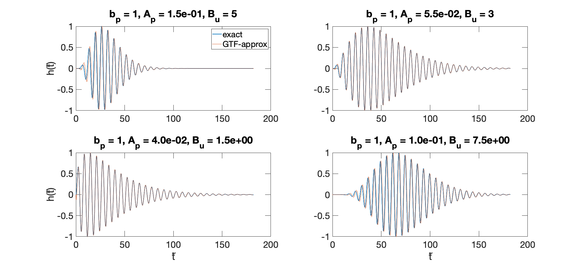
Figure 5: Comparison between the exact expression for impulse responses and its gammatone approximation For various values of model constants, the figure shows the comparison between $h(\tilde{t})$ (solid blue lines) as a function of normalized time $\tilde{t}=2\pi\text{CF}(x)t$ with $b_{p}=1$ and its highest order term approximation, $h_{GTF}$ of equation 17 (dotted red lines), which is simply a single gammatone filter (GTF) with tonal component $\cos(\tilde{t}_{b}-B_{u}\frac{\pi}{2})$, and allowing for half-integer $B_{u}$. The top figure panels is for integer $B_{u}$, and the bottom panels are for half-integer-$B_{u}$. As demonstrated in the figures, the model pressure impulse response is well-approximated by the highest-order term for small $A_{p}$ (such as those that are relevant for humans) except at the very earliest times.

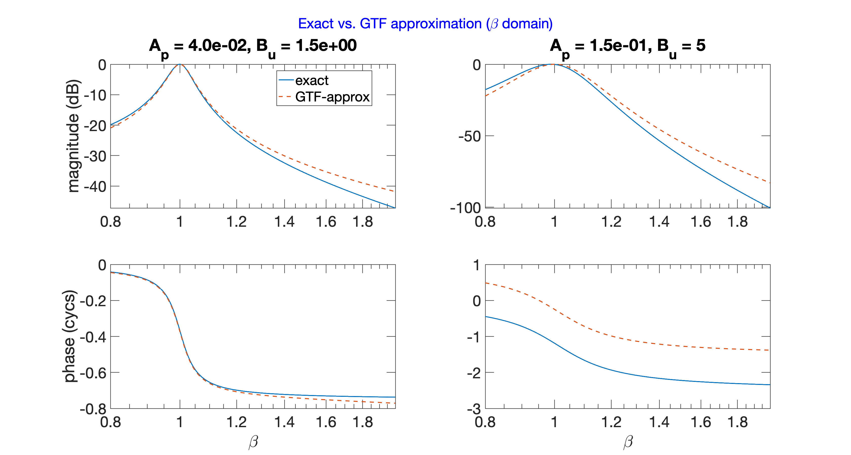
Figure 6: Comparison between the TFs for the exact expression for impulse responses and its gammatone approximation For a couple of values of model constants used in figure 5, the figure shows the comparison between the corresponding transfer functions for $h(\tilde{t})$ (solid blue lines) and its highest order term approximation, $h_{GTF}$ (dotted red lines). Comparing this figure with figure 5 shows that despite the exact and approximate impulse responses only differing at earlier times, their transfer functions for certain values of model constants (right) may differ outside the peak region.

Therefore, $h(\tilde{t})$ may be approximated using only the exponential factor and the highest order polynomial term. Hence, for $b_{p}=1$, we can write,

$$h(\tilde{t})\mathrel{\vbox{ \offinterlineskip\halign{\hfil$#$\cr\propto\cr\kern 2.0pt\cr\sim\cr\kern-2.0pt\cr}}}e^{-A_{p}\tilde{t}}\tilde{t}_{b}^{B_{u}-1}\cos(\tilde{t}_{b}-B_{u}\frac{\pi}{2})\;,\quad\text{with }B_{u}\in\mathbb{Z}>1\;.$$ (14)

Consequently, the behavior of our model $g(x,t)$ is qualitatively similar to the original Gamma-Tone-Filter (GTF) which was developed purely from a filter perspective and has no bases in cochlear physics. The GTF has a representation $at^{n-1}e^{-2\pi bt}\cos(2\pi ft+\phi)$ at each individual location [32] and is the basis on which a variety of filters in the gammatone family were developed.

From our expressions for impulse responses, and as illustrated in the top panels of figure 4, we may make the following comments regarding model behavior and its dependence on model constants:

• $b_{p}$ specifies the tonal frequency of the impulse response. Specifically, this is $f=\frac{\tilde{t}_{b}}{2\pi t}=\text{CF}(x)b_{p}$ as can be seen from the arguments of the $\sin,\cos$. When $b_{p}=1$, this is simply the characteristic frequency of any particular location, as dictated by the CF-map. This means that the frequency at which any location responds decrease with distance from the stapes.

• $A_{p}$ determines the decay of the envelope of the impulse response. This can be determined from the later parts of the response. Specifically, the decay factor at large times is, $=e^{-A_{p}\tilde{t}}=e^{-A_{p}2\pi\text{CF}(x)t}$. This means that for larger $A_{p}$, the decay at larger times is faster. In addition, the spatial dependence suggests that the decay at larger times is faster for locations closer to the stapes. When expressed in terms of period of the local CF, the decay time is constant assuming local scaling symmetry (locally spatially invariant model constant values)

• $B_{u}$ specifies the complexity of the impulse response. Specifically, it increases the number of polynomial terms, $\tilde{t}_{b}^{k}$ and the degree of the polynomial.

• $B_{u}$ determines the phase shift of the oscillatory factor of the impulse response.

• Both $B_{u}$ and $A_{p}$ specify the time at which the envelope of the impulse response peaks which occurs at $\tilde{t}=\frac{B_{u}-1}{A_{p}}$ (which is independent of location, if we assume scaling symmetry). Locally - or in the case of constant $A_{p},B_{u}$ along the length of the cochlea, the time, $t$, at which the envelope peaks is inversely proportional to $\text{CF}(x)$. Under these conditions, higher frequencies, which have maximal response in the base of the cochlear (closer to the stapes), peak faster than lower frequencies which have maximal response in the apex of the cochlear, further away from the stapes.

As mentioned previously, the impulse responses are useful for deriving parameterizations in terms of desired (or observed) time domain specifications for the impulse and step response - e.g. settling time. The impulse response representation is also used for convolution-based implementations. Furthermore, the impulse responses are useful for testing against experimental data as well as estimating values of model constants based on these experiments in order, for instance, to mimic processing of a particular species of interest.

There are currently no measurements of pressure impulse responses to test our model $g(x,t)$ with. However, we may compare our impulse response representation to impulse responses of basilar membrane velocity [33] and reverse-correlation data of auditory nerve fibers [34]. We expect that these measures are qualitatively (though not quantitatively) similar based on the qualitative similarity of their frequency domain responses. The model impulse response is qualitatively consistent with these measurements in which the response envelop grows, then decays asymmetrically. However, while our linear model predicts an oscillatory factor with a single frequency, the measurements [33, 34] suggest a glide settling at a dominant frequency being that predicted by our model. Future comparison of our model against impulse response-like data would add an additional dimension to our model tests. Similar to other comparisons, these tests would be useful in determining constraints on model constant values as well as in guiding how to best modify the model (e.g. forms of nonlinearity).

IV-B Generalization to half-integer-$B_{u}$

Here we generalize our expressions for the GAF impulse response to half-integer-$B_{u}$ cases in order to expand the variety of behavior which the filters may display. Once we reduce the integer restriction on $B_{u}$ to $B_{u}=\frac{n}{2}$ with $n\in\mathbb{Z}^{+}$, we find that we may lessen the restriction on the values of $B_{u}$ which result in desirable impulse response behavior. In this case, the condition for having an $h(\tilde{t})$ that has an envelope that grows then decays becomes $B_{u}\geq\frac{3}{2}$ rather than the more stringent condition required when $B_{u}$ is restricted to integer values, $B_{u}\geq 2$.

For integer and half-integer values of $B_{u}$ , we find that we may express the $h$ of the impulse response of the normalized pressure as,

$$h(\tilde{t})\propto e^{-A_{p}\tilde{t}}\tilde{t}^{B_{u}-\frac{1}{2}}J_{B_{u}-\frac{1}{2}}(\tilde{t}_{b})\;,$$ (15)

which is a generalization appropriate for both integer and half-integer-$B_{u}$. The above expression in terms of: Bessel functions of the first kind (which are decaying oscillatory functions), a decaying exponential factor, and a growth factor due to polynomials of $\tilde{t}$. We illustrate this in figure 4 (bottom panel), and provide the expressions including the scaling factors for a few instances in table II.

$\mathbf{B_{u}}$	$\mathbf{h(\tilde{t})=}$
$\frac{3}{2}=1.5$	$\frac{1}{b_{p}}e^{-A_{p}\tilde{t}}\tilde{t}J_{1}(\tilde{t}_{b})$
$\frac{5}{2}=2.5$	$\frac{1}{3b_{p}^{2}}e^{-A_{p}\tilde{t}}\tilde{t}^{2}J_{2}(\tilde{t}_{b})$
$\frac{7}{2}=3.5$	$\frac{1}{15b_{p}^{3}}e^{-A_{p}\tilde{t}}\tilde{t}^{3}J_{3}(\tilde{t}_{b})$
$\frac{9}{2}=4.5$	$\frac{1}{105b_{p}^{4}}e^{-A_{p}\tilde{t}}\tilde{t}^{4}J_{4}(\tilde{t}_{b})$

TABLE II: $h(\tilde{t})$ expressions (table I), for several cases of positive half-integer values of $B_{u}$. Note that the Bessel function of the first kind, $J_{\nu}(\tilde{t}_{b})$ provides decaying oscillatory terms. The half-integer value $B_{u}=\frac{1}{2}$ is not appropriate as it results in $e^{-A_{p}\tilde{t}}J_{o}(\tilde{t}_{b})$ in which the envelop only decays contrary to the desired behavior of the cochlea and auditory filters.

As may be inferred from the similarity in behavior, we may extend the approximation using GTFs to cases with half-integer-$B_{u}$ (as shown in figure 5), and consequently, we extrapolate the term GTFs to include non-integer-$B_{u}$,

$$h(\tilde{t})\mathrel{\vbox{ \offinterlineskip\halign{\hfil$#$\cr\propto\cr\kern 2.0pt\cr\sim\cr\kern-2.0pt\cr}}}h_{GTF}(\tilde{t})$$ (16)

$$h_{GTF}\propto e^{-A_{p}\tilde{t}}\tilde{t}^{B_{u}-\frac{1}{2}}\cos(\tilde{t}_{b}-B_{u}\frac{\pi}{2})\;,$$ (17)

We expect that $h_{GTF}$ is a good approximation of GAFs with real $B_{u}$ and not just integer and half-integer-$B_{u}$. Once we remove the restriction of integer $B_{u}$, we can achieve tonal component that is not only restricted $\sin(\tilde{t}_{b})$ or $\cos(\tilde{t}_{b})$, but rather may have a larger variety of phases. This is particularly clear from equation 17. Figure 4 illustrates the variation of phase of the tonal component with $B_{u}$ and shows that, once we reduce the integer condition, it is not restricted to $\sin(\tilde{t}_{b})$ or $\cos(\tilde{t}_{b})$.

V ODEs for Integer $B_{u}$

Here we derive the ODE representation for GAFs. Transforming equation 11 for $\frac{P(x,\omega)}{C(x)}$ into the time domain yields a linear ODE of order $2B_{u}$,

$$\bigg{(}\frac{d^{2}}{d\tilde{t}^{2}}+2A_{p}\frac{d}{d\tilde{t}}+|p|^{2}\bigg{)}^{B_{u}}q(x,t)=u(t)\;,$$ (18)

where $v_{st}(\omega)\xleftrightarrow{}u(t)$, $\frac{P(x,\omega)}{C(x)}\xleftrightarrow{}q(x,t)$, and $\frac{d}{d\tilde{t}}=\frac{1}{2\pi\text{CF}(x)}\frac{d}{dt}$. Neglecting matters of computational expense, the ODE may be formulated and simulated in a variety of ways and may be run in real time. For instance a state space formulation (with $\sum\limits_{i=1}^{M}(2{B_{u}}_{,i}-1)$ state variables where $M$ is the number of locations/filters) with Runge-Kutta methods for solution is quite accurate.

One approach for simulations which we use to generate the responses in section VII is to express the problem in state space representations translated from the ODE of equation 18 (or the TF of equation 11) and then use Runge-Kutta based ODE solvers. The state space representation we use for the $i^{th}$ filter in the filterbank or at a fixed location, $x_{i}$, may be expressed as follows for the example case of $B_{u}=2$. As we’re interested in demonstrating the response at a single location here, we may simply consider the variable in terms of $\tilde{t}_{i}$ rather than $t$ and $x$, and accordingly, we may simulate in $\tilde{t}_{i}$. Hence, we use, $\mathtt{u}(\tilde{t}_{i})=u(\frac{\tilde{t}_{i}}{2\pi\mathrm{CF}(x_{i})})$ and $\mathtt{q}(\tilde{t}_{i})=q(t,x_{i})$.

$$\frac{d}{d\tilde{t}_{i}}\vec{z}(\tilde{t}_{i}) =\begin{bmatrix}&1&&\\ &&1&\\ &&&1\\ -4A_{p}&-4A_{p}^{2}-2|p|^{2}&-4A_{p}|p|^{2}&-|p|^{4}\end{bmatrix}\vec{z}(\tilde{t}_{i})$$ (19)

$$+\begin{bmatrix}0\\ 0\\ 0\\ 1\end{bmatrix}\mathtt{u}(\tilde{t}_{i}),\quad\vec{z}(0)=\vec{0}\;,$$

The first state variable in $\vec{z}$ is the output solution $\mathtt{q}(\tilde{t}_{i})$. As we solve the state-space representation numerically, this representation is essentially in discrete time due to the nature of simulations and numerical ODE solvers.

The ODE representation is particularly easy and direct and appropriate for software implementations for certain classification applications and perceptual studies - presuming they are interested in filters with a set value for $B_{u}$. Additionally, we may directly modify the ODE to incorporate additional behavior. One example is incorporating nonlinearity directly by making the coefficients dependent on $q$, rather than using the existing compression schemes. The ODE representation may also directly be modified to incorporate other behavior such as memory, rectifier, refraction period, and various other mechanical and neural effects potentially by extensions to deterministic and stochastic delay-differential equations [35, 36, 37, 38].

Despite its suitability for simple direct implementations and for incorporating additional behavior, the ODE representation is the most constraining in terms of possible values of $B_{u}$ as our formulation restricts it to integer values - though we do use it in the next section, to set us up for our integral formulation which is not limited to the integer-$B_{u}$ case. We may be able to extend the representation to non-integer-$B_{u}$ cases using fractional calculus methods but this is beyond the scope of this paper.

VI Integral Expressions

Here, we take another approach for deriving real time representations that involve integration and which we develop using differential operator theory [39]. We first derive the integral representation for integer-$B_{u}$ filters, then present the integral representations for the rational-$B_{u}$ case.

VI-A Integer $B_{u}$

Defining the differential operator,

$$\tilde{D}\triangleq\frac{d}{d\tilde{t}}=\frac{1}{2\pi\text{CF}(x)}\frac{d}{dt}\;,$$ (20)

we may express, $q(x,t)$ of equation 18 as,

$$q(x,t;B_{u},A_{p},b_{p};u(t))=\bigg{(}\frac{1}{(\tilde{D}-p)(\tilde{D}-\overline{p})}\bigg{)}^{B_{u}}u(t)\;.$$ (21)

As we are interested in the solution with zero initial conditions in response to any smooth function $u(t)$, let us define our integration operator as,

$$\frac{1}{\tilde{D}_{o}}f(\tilde{t})\triangleq\int_{0}^{\tilde{t}}{f(\tilde{t}^{\prime})}d{\tilde{t}^{\prime}}=2\pi\text{CF}(x)\int_{0}^{t}{g(t^{\prime})}d{t^{\prime}}\;.$$ (22)

While we have deviated from the classical formulation of differential operator theory, dealing with these definite integrals provides the analytic expressions for the desired solutions directly rather than dealing with an indefinite integral then solving for the constants using initial conditions. Also, note that equation 22 does not correspond to the zero initial condition case for inputs that are impulses and other generalized functions.

Using the above formula, we may express the response as follows by using differential operator theory:

$$q(x,t;B_{u},A_{p},b_{p};u(t)) =\bigg{(}\frac{1}{(\tilde{D}_{o}-p)(\tilde{D}_{o}-\overline{p})}\bigg{)}^{B_{u}}u(t)$$ (23)

$$=\bigg{(}\frac{1}{\tilde{D}_{o}-\overline{p}}\bigg{)}^{B_{u}}\bigg{(}\frac{1}{\tilde{D}_{o}-p}\bigg{)}^{B_{u}}u(t)$$

$$=e^{\overline{p}\tilde{t}}\bigg{(}\frac{1}{\tilde{D}_{o}}\bigg{)}^{B_{u}}e^{-\overline{p}\tilde{t}}e^{p\tilde{t}}\bigg{(}\frac{1}{\tilde{D}_{o}}\bigg{)}^{B_{u}}e^{-p\tilde{t}}u(t)$$

$$=e^{\overline{p}\tilde{t}}\bigg{(}\frac{1}{\tilde{D}_{o}}\bigg{)}^{B_{u}}e^{2ib_{p}\tilde{t}}\bigg{(}\frac{1}{\tilde{D}_{o}}\bigg{)}^{B_{u}}e^{-p\tilde{t}}u(t)\;,$$

which, despite its intermediate operations, results in a real output for any given real input. As an example, for the case of $B_{u}=1$, this yields,

$$q(x,t;1,A_{p},b_{p};u(t))=\bigg{(}2\pi\text{CF}(x)\bigg{)}^{2}e^{2\pi\text{CF}(x)\overline{p}t}\times$$ (24)

$$\int_{0}^{t}{e^{4\pi\text{CF}(x)ib_{p}t^{\prime}}\int_{0}^{t^{\prime}}{e^{-2\pi\text{CF}(x)pt^{\prime\prime}}u(t^{\prime\prime})}d{t^{\prime\prime}}}d{t^{\prime}}\;,$$

For more reasonable values of integer $B_{u}$, each $\big{(}\frac{1}{\tilde{D}_{o}}\big{)}^{B_{u}}$ of equation 23 results in nested integrals,

$$\bigg{(}\frac{1}{\tilde{D}_{o}}\bigg{)}^{B_{u}}f(\tilde{t})=\int_{0}^{\tilde{t}}d{\tilde{t}^{\prime}}{\int_{0}^{\tilde{t}^{\prime}}d{\tilde{t}^{\prime\prime}}{\dots\int_{0}^{t^{(B_{u}-1)}}d{\tilde{t}^{(B_{u})}}{f(\tilde{t}^{(B_{u})})}}}\;.$$ (25)

It is possible to compute solutions $q$ for a given input $u$, for the case of integer $B_{u}$, directly using equations 23 and 25. However, it is cumbersome, and has a form (or number of nested integrals) based on the value of $B_{u}$. Therefore, we simplify these operations into two integrals using the Cauchy formula for repeated integration which is valid for integer $B_{u}$ [40, 41]. This allows us to express equation 23 using,

$$\bigg{(}\frac{1}{\tilde{D}_{o}}\bigg{)}^{B_{u}}f(\tilde{t})=\frac{1}{(B_{u}-1)!}\int_{0}^{\tilde{t}}{(\tilde{t}-\tau)^{B_{u}-1}f(\tau)}d{\tau}\;,$$ (26)

This allows us to derive the following equivalent to equation 23 that simplifies the problem to only two nested integrals regardless of the value of $B_{u}$,

$$\mathtt{q}(\tilde{t}_{i};B_{u},A_{p},b_{p};\mathtt{u}(\tilde{t}_{i}))=\bigg{(}\frac{1}{(B_{u}-1)!}\bigg{)}^{2}e^{\overline{p}\tilde{t}_{i}}\times$$ (27)

$$\int_{0}^{\tilde{t}_{i}}{d\tau}(\tilde{t}_{i}-\tau)^{B_{u}-1}e^{2ib_{p}\tau}\int_{0}^{\tau}{dT}{(\tau-T)^{B_{u}-1}e^{-pT}\mathtt{u}(T)}\;,$$

for integer values of $B_{u}$. While it is appropriate to express this in the $t$ domain, for a given filter, we express this in the $\tilde{t}_{i}$ domain for compactness. We use the notation $\mathtt{q}$ for $\mathtt{q}(\tilde{t}_{i})=q(x_{i},t)$ and $\mathtt{u}$ for $\mathtt{u}(\tilde{t}_{i})=u(t(\tilde{t}_{i},x_{i}))=u(\frac{\tilde{t}_{i}}{2\pi\textrm{CF}(x_{i})})$.

For a smooth function for the input this provides the full solution (including both the complementary and particular solutions) when the initial conditions are all zero. If $u(t)=\delta(t)$, the expressions result in the full solution with all initial conditions being zero with the exception of the initial condition corresponding to the highest derivative which is unity. Notice that using the integral representation with $u(t)=\delta(t)$ directly results in our expressions for the impulse responses for normalized pressure, $g(x,t)=2\pi\text{CF}(x)h(\tilde{t})$. This can most easily be checked with $B_{u}=1$.

In the above expression, a parameter of the integrand also appears as an upper limit of integration. We therefore provide an alternative equivalent expression by using,

$$\int_{0}^{y}{f(z;y)}d{z}=y\int_{0}^{1}{f(Zy;y)}d{Z}\;,$$ (28)

where we perform the change of variables from $z$ to $Z$ such that $z=Zy$, resulting in a definite integral with a numerical value for the limits of integration. This results in the following expression for $\mathtt{q}(\tilde{t}_{i})$ - where we have dropped the subscript $i$ to reduce clutter,

$$\mathrm{q}(\tilde{t};B_{u},A_{p},b_{p};\mathrm{u}(\tilde{t}))=$$ (29)

$$\bigg{(}\frac{1}{(B_{u}-1)!}\bigg{)}^{2}e^{\overline{p}\tilde{t}}\int_{0}^{1}{d\zeta}\tilde{t}^{B_{u}}(1-\zeta)^{B_{u}-1}\times$$

$$e^{2ib_{p}\tilde{t}\zeta}\int_{0}^{1}{d\chi}{(\tilde{t}\zeta)^{B_{u}}(1-\chi)^{B_{u}-1}e^{-p\tilde{t}\zeta\chi}\mathrm{u}(\tilde{t}\zeta\chi)}$$

$$=\frac{\tilde{t}^{2B_{u}}}{\bigg{(}(B_{u}-1)!\bigg{)}^{2}}e^{\overline{p}\tilde{t}}\int_{0}^{1}{d\zeta}(1-\zeta)^{B_{u}-1}\zeta^{B_{u}}\times$$

$$e^{2ib_{p}\tilde{t}\zeta}\int_{0}^{1}{d\chi}{(1-\chi)^{B_{u}-1}e^{-p\tilde{t}\zeta\chi}\mathrm{u}(\tilde{t}\zeta\chi)}\;.$$

Both equations 27 and 29 are integration-based expressions that may be used to evaluate the responses to a given input signal. Importantly, $B_{u}$ occurs only as any other constant parameterizing the expression. Consequently, the same expression may be used regardless of the value of $B_{u}$. It is also important to note that any integrator-based implementation of the representations in this section must have the capacity of handling complex numbers as part of the intermediate operations.

VI-B Rational $B_{u}$

We extend the representation to cases where $B_{u}$ is rational (if not real). Just as we used the Cauchy formula for repeated integrals for integer $B_{u}$ to derive a simple integral representation, here we use its generalization to non-integrals, the Riemann–Liouville integral in order to generalize our expression for $q$ to rational $B_{u}$ for the case of zero initial conditions as detailed in this section. Utilizing the Riemann–Liouville fractional integral operator [40, 41] results in the following solution parallel to equations 27 and 29. Note that since we deal with zero initial conditions, we do not need to be concerned with the various types of integral expressions for fractional derivatives.

$$\mathrm{q}(\tilde{t};B_{u},A_{p},b_{p};\mathrm{u}(\tilde{t}))=$$ (30)

$$\bigg{(}\frac{1}{\Gamma(B_{u})}\bigg{)}^{2}e^{\overline{p}\tilde{t}}\int_{0}^{\tilde{t}}{d\tau}(\tilde{t}-\tau)^{B_{u}-1}\times$$

$$e^{2ib_{p}\tau}\int_{0}^{\tau}d{T}{(\tau-T)^{B_{u}-1}e^{-pT}\mathrm{u}(T)}$$

$$=\frac{\tilde{t}^{2B_{u}}}{\bigg{(}\Gamma(B_{u})\bigg{)}^{2}}e^{\overline{p}\tilde{t}}\int_{0}^{1}d\zeta(1-\zeta)^{B_{u}-1}\zeta^{B_{u}}\times$$

$$e^{2ib_{p}\tilde{t}\zeta}\int_{0}^{1}d\chi(1-\chi)^{B_{u}-1}e^{-p\tilde{t}\zeta\chi}\mathrm{u}(\tilde{t}\zeta\chi)\;.$$

In figure 7, we demonstrate that we can use the integral expressions to compute the response to a quadratic chirp for the case of non-integer $B_{u}$. The solution behaves as expected in that it responds maximally to frequencies close to the filter’s peak frequency (with some delay).

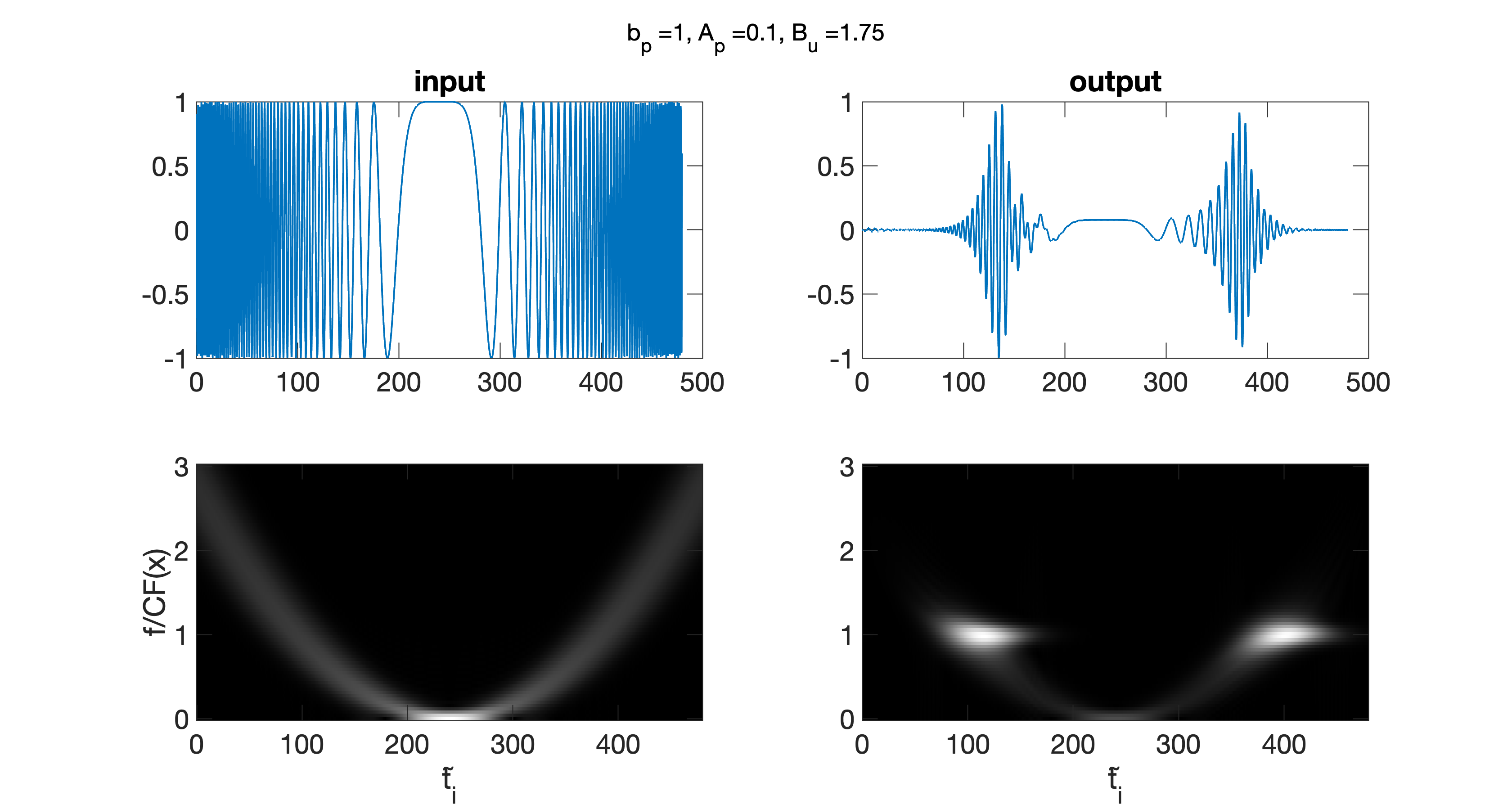
Figure 7: The integral expressions can be used to compute responses for the case of fractional-$B_{u}$ GAFs: The figure shows the normalized output, $q$ (top right) at any filter $i$ or equivalently a specified location with characteristic frequency $\textrm{CF}(x_{i})$. The output is plotted as a function of scaled time, $\tilde{t}_{i}=2\pi\textrm{CF}(x_{i})t$ for the $i^{th}$ filter, in response to a quadratic chirp. The quadratic chirp used as the input (top left) has a decaying then increasing instantaneous frequency. The input and output are plotted as a function of scaled time: $\mathtt{u}(\tilde{t}_{i})\triangleq u(t(x_{i},\tilde{t}_{i}))$, and the response $\mathtt{q}(\tilde{t}_{i})\triangleq q(t,x_{i})$. The response is computed using the integral expression. The figure also shows the spectrogram of both the input (bottom left) and normalized pressure response (bottom right). The plots show that filter primarily responds (with a time delay - dependent on $A_{p}$ and $B_{u}$ values) to instantaneous frequencies that are at, and near, the characteristic frequency. It is relatively insensitive to frequencies further away from the characteristic frequency.

The integral representation is real time and is in itself a continuous time rather than discrete time formulation. It provides analytic expressions to be evaluated (rather than equations to be solved) for direct solutions to any input $u(t)$ that are evaluated via simple operations such as exponentiation and integration and is possible because the system is LTI. The error for digital software implementations is due to the chosen integration scheme. There are no derivatives involved as the pressure filter is all-pole. This is desirable as taking derivatives of noisy data should be avoided. Note that the $V$ filter can also be expressed without taking any derivatives as it only has a single zero corresponding to a first derivative of $u(t)$ which can be avoided by using integration by parts in the innermost integral.

One apparent virtue of this formulation in continuous time is studying analytic solutions in response to certain types of inputs $u(t)$ - e.g. tones, impulses, vowels with analytic representations in time domain, as a function of parameters and locations (or their CF). This may be potentially be coupled with analytic models of higher processing in the auditory system for perceptual studies. Software implementations, which are the implementation of choice for perceptual studies, are quite easy to implement for the integral representation.

We are unaware of representations for any filters that use this approach which may prove useful for other types of filters. The integral representation can be directly extended to any all-pole filter.

VII Equivalence of Representations

In this section, we test our derivations and demonstrate that our representations are consistent with one another. We do this by using the various representations to compute the response of a single filter to an input $\mathtt{u}(\tilde{t})$ (where we have dropped the previously-used filter-specific subscript $i$ in $\tilde{t}_{i}$ for simplicity). We carry out the equivalence tests for a case of integer $B_{u}$ to compare all representations and a case of half-integer $B_{u}$ to compare all representations except for the ODE formulation which is limited to integer-$B_{u}$. In both cases, we choose our inputs such that the input and output have analytic expressions in the time in frequency domains. This allows us to generate analytic solutions to compare the outputs of the various methods against.

VII-A Integer-Exponent

For the integer-$B_{u}$ case, we compare the outputs of the various methods in response to an input,

$$\mathtt{u}(\tilde{t})=\tilde{t}\cos(10\tilde{t})e^{-\frac{\tilde{t}}{2}}+\tilde{t}^{3}e^{-\tilde{t}}\cos(\tilde{t})\;.$$ (31)

The outputs generated using the various representations are shown in figure 8. The figure shows that the responses computed using the ODE and integral representations for the case of an integer $B_{u}$ are equal. We also include the responses generated analytically from using the TF/impulse representation rather than include numerically computed responses from those representations in order to isolate any potential differences due to the representations themselves rather than avoid any differences that may occur due to numerical processing choices needed for the TF and impulse response computations.

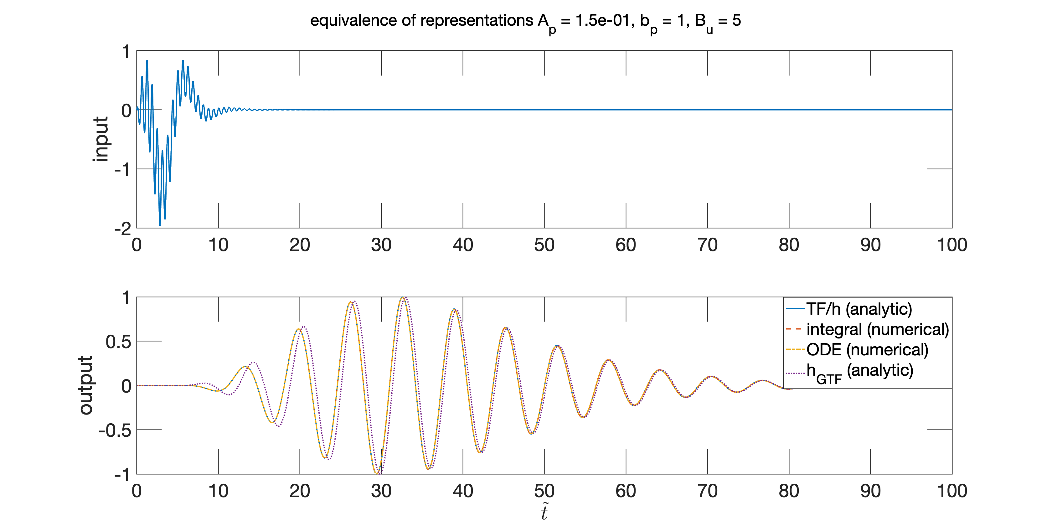
Figure 8: The GAF representations are equivalent for the case of integer $B_{u}$: The figure shows the normalized model output of a single filter with a specified peak frequency, or equivalently (from the perspective of cochlea models), at specified location with characteristic frequency $\textrm{CF}(x_{i})$. The output, $\mathtt{q}(\tilde{t}_{i})$ is plotted as a function of scaled time at a particular location, $\tilde{t}_{i}=2\pi\textrm{CF}(x_{i})t$, in response to the input (top figure). As we are interested in displaying the response response only at a single location, we have represented the input and response in scaled time, $\mathtt{u}(\tilde{t}_{i})\triangleq u(t(x_{i},\tilde{t}_{i}))$, and the response $\mathtt{q}(\tilde{t}_{i})\triangleq q(t,x_{i})$. The response (bottom figure) is computed numerically using the integral representation (dashed red line) and the ODE representation with zero initial conditions (dash-dotted yellow line), and analytically using the TF or impulse response representation (solid blue line) as well as the GTF approximation (dotted purple line). The responses from the various representations are equivalent for integer $B_{u}$, with the exception of the response using the GTF approximation which deviates from the exact response for the selected set of model constant values (more so at small times).

We also include the response generated using the $h_{GTF}$ approximation (generated analytically). The figure shows that, at least for integer-$B_{u}$, all exact GAF representations are equivalent. Additionally, the response generated using $h_{GTF}$ is qualitatively consistent with the exact solution. Quantitatively - for the set of chosen model constant values, it does show small deviations particularly earlier in time. Consequently, for such implementations, differentiating between GAFs and GTFs (and other filters in the gammatone family) and restricting ones-self to a particular filter is not fruitful.

VII-B Half-Integer-Exponent

In figure 9, we compare the responses for the case of half-integer $B_{u}$ to an input,

$$\mathtt{u}(\tilde{t})=e^{-A_{p}\tilde{t}}\tilde{t}^{a-\frac{1}{2}}J_{a-\frac{1}{2}}(\tilde{t}_{b})\quad\text{with }a=\frac{1}{2}\;,$$ (32)

which has a transfer function - neglecting the gain constant, represented by $\big{(}s^{2}+2A_{p}s+A_{p}^{2}+b_{p}^{2}\big{)}^{-a}$. We choose the input to have the same base TF as the GAF (i.e. same $A_{p},b_{p}$ but any positive exponent) so that we may analytically derive the true solution that we use to compare the outputs from the other representations against.

The outputs are generated analytically using the TF or impulse response representation and numerically using the integral representation. The figure shows that the outputs computed integral representation are equivalent to those generated analytically. Additionally, we numerically compute the responses using the TF representation with FFTs/IFFTs and show that they diverges from that generated analytically using the same representation - in contrast to the integral methods. This may be a result of: additional numerical processing requirements for computing the response using TFs and FFTs/IFFTs; and the fundamental difference between the assumed nature of signals - in terms of being periodic and discrete, for which Discrete Fourier Transforms (used to generated the soltion with FFT/IFFT algorithms) are appropriate compared to which the Fourier Transforms (used to derive the true/analytic solution) are appropriate.

Consequently, for digital software implementations, we encourage the use of the integral representation which is not only accurate, real-time (if using efficient integration algorithms), and appropriate for non-integer exponent GAFs, but also does not require any preprocessing choices - unlike TFs and impulse responses, which cause the computed output to diverge from the analytic solution - as illustrated in the figure. These observations not only apply for software implementations of GAFs, but also directly translate to other filters for which the base filter may be represented as all-pole rational transfer functions.

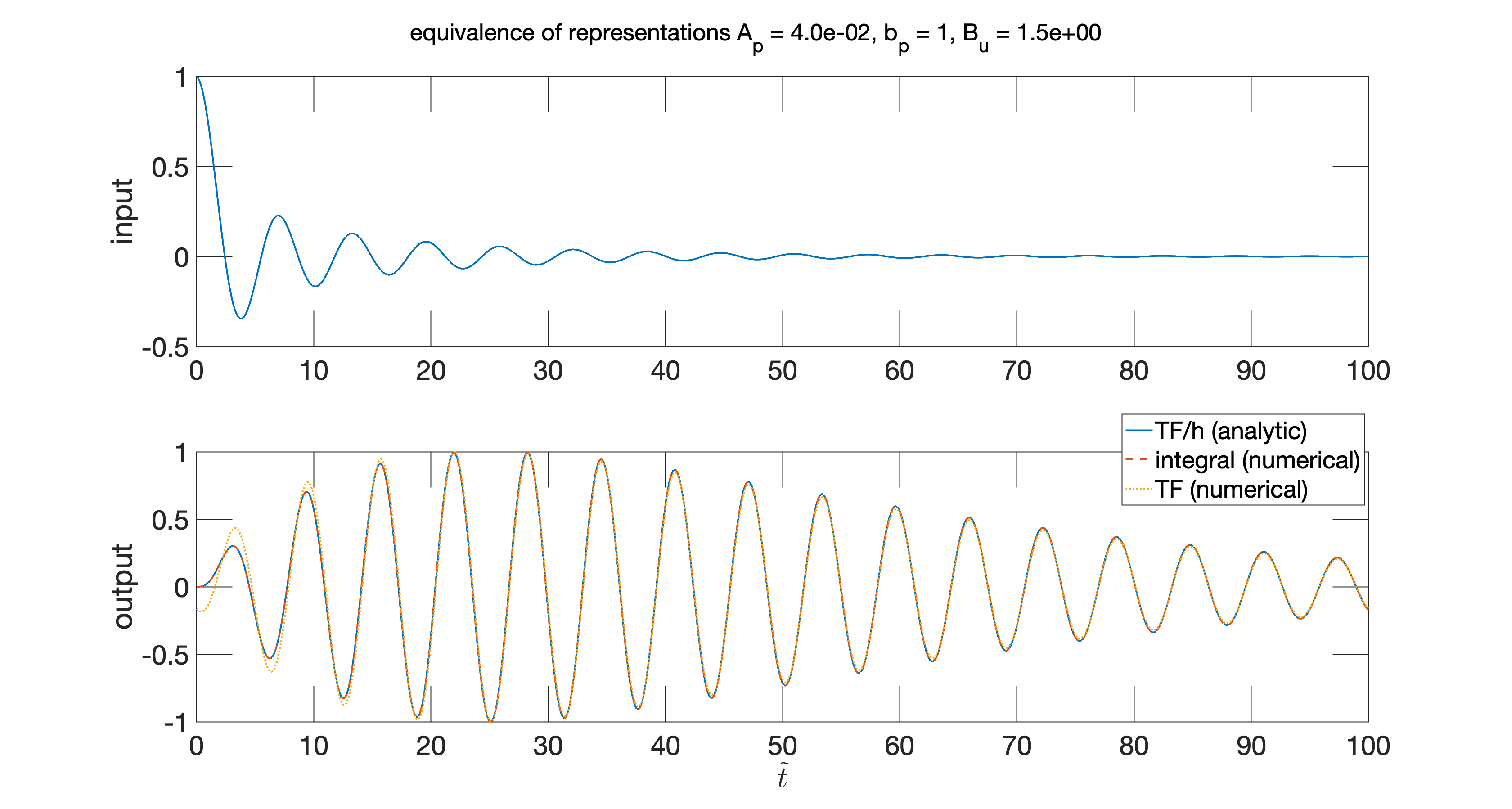
Figure 9: The GAF integral representation accurately computes the response for half-integer-exponent filters: Similar to figure 8, we plot the normalized response of a filter to an input (top figure) using various methods for computing the output. However, in this figure, the filter has a half-integer-$B_{u}$. The output computed numerically using the integral representation (dashed red line) is equivalent to the analytic solution generated using the TF/h representations (solid blue line). On the other hand, the computational implementation of the TF representation (using FFTs) result in deviations (particularly visible at smaller times) from the true solution. This suggests that the integral expressions may be considered more desirable for software implementations in the sense that it does not require additional processing beyond evaluating the integral expression - and hence is more accurate.

VIII Conclusions and Future Directions

VIII-A Conclusions

In this paper, we presented rational-exponent GAFs. These filters and filterbanks are useful for an array of signal processing applications. Due to their relationship to an underlying cochlear model, they are also useful for mechanistic studies of the auditory system. Generalizing the filters to rational-$B_{u}$ cases, as we have done here, allows for achieving a wider variety of filter behavior. Additionally, it allows for more accurately estimating mechanistic variables underlying signal processing behavior in the associated cochlea model. We derived equivalent representations in the frequency and time domains - transfer functions, impulse responses, ODEs, and integral expressions. Each of the various representations is appropriate for different uses: e.g. testing model accuracy against various experimental datasets, or parameter estimation to match processing from said datasets; extensions to incorporate nonlinearity and neural processing; filter-specification-based parameterization for apriori control of filter behavior based on desired peak frequencies, quality factors, settling times, etc; architecture, implementation, and processing requirements. To test that we have properly derived the various representations, we examined the responses to the same input using the various representations, and studied - in section VII, the consistency of the various representations with one another when used to generate outputs.

VIII-B Future Directions

Future directions may include pursuing some of the directions enabled by having rational-$B_{u}$ filters and associated cochlear models, as well as directions enabled by each of the representations presented in this paper.

VIII-B1 Extensions to Other Filters

We have presented rational-exponent filters that consist of a second-order filter - as a base, raised to a rational number. The fundamental methods that we used to derive the rational-exponent representations for this filter in this paper may be extended to derive other rational-exponent filters building on various types of base filters. A related example from existing work may be expressed in the form $(\frac{1}{s+\tau})^{B_{u}}$ with a low-pass RC circuit $\frac{1}{s+\tau}$ for its base filter [10]. We recommend restricting the base filters (which are then to be raised to a rational exponent) to fourth-order filters (or otherwise higher order filters with special forms) such that pole placement to achieve a stable system is simple - recall that the stability of the rational-exponent filter is based entirely on that of the base filter.

VIII-B2 Applications and Implementations

The time domain representations can translated for corresponding digital filters using standard methods used for classical filters represented by rational transfer functions. Additional work is needed towards digital implementations of the transfer function representation.

Future directions also involve pursuing some of the applications mentioned in section I using our filters and model that are relieved of the integer-$B_{u}$ restriction. Some of these applications may require deriving alternate parameterizations (e.g. based on desired or observed frequency-domain characteristics), selecting parameter values, developing architectures appropriate for certain implementations, or incorporating certain features such as nonlinearity or orthogonality. Once criteria, for instance, may be equal magnitudes of the $P$ filter variable for various filters in a filterbank - or equivalently at various locations along the length of the cochlea, which would inform any dependence of $C$ (or its equivalents in corresponding representations) on $x$.

VIII-B3 Parameterization

The transfer function representation allows for deriving parameterizations of GAF based on desired filter characteristics such as peak frequency, quality factor, and group delay. Similarly, the impulse response representation, and its integral, may be used for deriving parameterizations based on impulse or step response characteristics such as settling time, instantaneous frequency, and functions of the envelope shape. Such parameterizations are useful for easily designing the filters based on desired behavior rather than using a fixed set of generic values of constants. They are also useful in determining the relationship between characteristics of the filter variables (e.g. quality factor, group delay, peak frequency, rise time, settling time) and underlying mechanistic properties such as nominal stiffness and slope of negative damping and gain features, or indeed more interesting properties such as those relating to power flux into the traveling wave. Additionally, a combination of parametization using time and frequency domain characteristics provides a mapping between characteristics in the time and those in the frequency domain which would be useful for building intuition and a common framework for interpreting experiments in different domains - and consequently, common ground between experimentalists who use different methods.

VIII-B4 Incorporating Nonlinearity and Additional Behavior

The GAFs and the underlying mechanistic model are linear as is appropriate for mimicking cochlear processing of sounds at low stimulus levels. In order for the model to mimic such processing across stimulus levels, one may incorporate quasi-linearity (as is discussed in the literature) or nonlinearity. The latter is best incorporated in the ODE representation which is also the best representation for incorporating other such as memory as mentioned in section V. We note that incorporating nonlinearity and other behavior into the model response/filter variables may decouple the GAFs from its mechanistic and physics-based roots.

Appendix A Filter Choice

As mentioned in section I-C, our objective is to develop rational-exponent filters. In particular, we focused on developing rational-exponent GAFs which are filters and filterbanks with a second order rational transfer function as the base filter. In developing these filters, we present various equivalent time and frequency domain representations. To achieve our objective, we build on our previously developed auditory model (GAFs) [12] and introduce the rational-$B_{u}$ case of filters in their various time and frequency domain representations. We use this particular choice of auditory model due to the following reasons:

1. Given only the desired peak frequencies, all filters in the filterbank may - to first approximation, be parameterized by the same set of two constants ($A_{p},B_{u}$ of sections I and III). This is exact for the case of constant-Q filterbanks, and is a result of model construction in the normalized frequency domain. This greatly reduces the number of free parameters one must specify values for to only two constants - a much smaller number than other auditory filters.

2. The GAFs may be parameterized in terms of characteristics such as peak frequency, quality factors, and ratio of quality factor to normalized group delay rather than the generic model constants which is not the case for other filters and models [30, 9]. This allows us to control the specifications of the filter easily without requiring manual tuning or optimization. This is made possible due to the simplicity of the model variables and the small number of constants required for parameterization.

3. We have previously tested the GAFs and shown that they are able to mimic cochlear signal processing at low levels. We have tested the model against various experimental datasets (neural and mechanical, different animals, different locations along the length of the cochlea). This extent of testing has not been performed for other cochlear models or auditory filters.

4. Additionally, we have previously estimated various sets of model constant values to mimic processing of certain species including chinchilla and humans [12, 30]. Choosing filter constant values to mimic certain species may improve the performance of feature extraction paradigms in an application-dependent manner - e.g. bird sound classification, and digital stethoscopes.

5. GAFs bear certain similarities to related existing (non-mechanistic) auditory filters in the gammatone family of filters including the gammatone filter (GTF), the all-pole gammatone filter (APGF), and the one-zero gammatone filter (OZGF) which have been implemented with certain existing architectures that one may be able to leverage for implementing the GAFs presented here which is quite useful. Synthesis filters have also been constructed for GTFs [42] amongst other filters, which may guide development of synthesis filters for constructing analysis filters for integer and non-integer-$B_{u}$ GAFs. The similarities between these filters also implies that one may extend the derivations in this paper to other filters in the gammatone family.

6. The model doubles as an auditory filterbank and a mechanistic model of the mammalian cochlea and hence is useful for a variety of signal processing and peripheral auditory science applications. The response/filter variables (differential pressure across the Organ of Corti - OoC, OoC partition velocity) and mechanistic variables (differential pressure wavenumber, effective OoC impedance) that encode how the cochlea works are parameterized by the same (small) set of model constants. The parameterization of these variables by the same set of constants enables us to use knowledge of the frequency domain filter transfer function - or equivalently certain characteristics [30, 9] such as peak frequency, quality factor, and ratio of quality factor to group delay, to determine the mechanistic variables to study how the cochlea works in various animals and how it processes different frequencies and signals along its length.

References

- [1] I. Podlubny, Fractional differential equations: an introduction to fractional derivatives, fractional differential equations, to methods of their solution and some of their applications. Elsevier, 1998.
- [2] C. I. Muresan, I. R. Birs, E. H. Dulf, D. Copot, and L. Miclea, “A review of recent advances in fractional-order sensing and filtering techniques,” Sensors, vol. 21, no. 17, p. 5920, 2021.
- [3] J. Sang, H. Hu, I. M. Winter, M. C. Wright, and S. Bleeck, “The ‘neural space’: A physiologically inspired noise reduction strategy based on fractional derivatives,” in 2011 11th International Symposium on Communications & Information Technologies (ISCIT), pp. 512–517, IEEE, 2011.
- [4] A. Radwan, “Stability analysis of the fractional-order rlc circuit,” J. fract. calc. appl, vol. 3, no. 1, pp. 1–15, 2012.
- [5] A. G. Radwan, A. S. Elwakil, and A. M. Soliman, “Fractional-order sinusoidal oscillators: design procedure and practical examples,” IEEE Transactions on Circuits and Systems I: Regular Papers, vol. 55, no. 7, pp. 2051–2063, 2008.
- [6] D. Lin, X. Liao, L. Dong, R. Yang, S. Y. Samson, H. H.-C. Iu, T. Fernando, and Z. Li, “Experimental study of fractional-order rc circuit model using the caputo and caputo-fabrizio derivatives,” IEEE Transactions on Circuits and Systems I: Regular Papers, vol. 68, no. 3, pp. 1034–1044, 2021.
- [7] M. S. Sarafraz and M. S. Tavazoei, “Realizability of fractional-order impedances by passive electrical networks composed of a fractional capacitor and rlc components,” IEEE Transactions on Circuits and Systems I: Regular Papers, vol. 62, no. 12, pp. 2829–2835, 2015.
- [8] M. Tavakoli-Kakhki, M. Haeri, and M. S. Tavazoei, “Notes on the state space realizations of rational order transfer functions,” IEEE Transactions on Circuits and Systems I: Regular Papers, vol. 58, no. 5, pp. 1099–1108, 2010.
- [9] S. A. Alkhairy, “Characteristics-based design of multi-exponent bandpass filters,” IEEE Transactions on Circuits and Systems I: Regular Papers, submitted.
- [10] T. Hélie, “Simulation of fractional-order low-pass filters,” IEEE/ACM Transactions on audio, speech, and language processing, vol. 22, no. 11, pp. 1636–1647, 2014.
- [11] R. F. Lyon, “All-pole models of auditory filtering,” Diversity in auditory mechanics, pp. 205–211, 1997.
- [12] S. A. Alkhairy and C. A. Shera, “An analytic physically motivated model of the mammalian cochlea,” The Journal of the Acoustical Society of America, vol. 145, no. 1, pp. 45–60, 2019.
- [13] C. J. Galbraith, R. D. White, L. Cheng, K. Grosh, and G. M. Rebeiz, “Cochlea-based rf channelizing filters,” IEEE Transactions on Circuits and Systems I: Regular Papers, vol. 55, no. 4, pp. 969–979, 2008.
- [14] R. Marrocchio, A. Karlos, and S. Elliott, “Waves in the cochlea and in acoustic rainbow sensors,” Wave Motion, vol. 106, p. 102808, 2021.
- [15] T. Jiang and J. Zheng, “Automatic phase picking from microseismic recordings using feature extraction and neural network,” IEEE Access, vol. 8, pp. 58271–58278, 2020.
- [16] X. Zeng and S. Wang, “Underwater sound classification based on gammatone filter bank and hilbert-huang transform,” in 2014 IEEE International Conference on Signal Processing, Communications and Computing (ICSPCC), pp. 707–710, IEEE, 2014.
- [17] J. Yao and Y.-T. Zhang, “The application of bionic wavelet transform to speech signal processing in cochlear implants using neural network simulations,” IEEE Transactions on Biomedical Engineering, vol. 49, no. 11, pp. 1299–1309, 2002.
- [18] T. Zhang, F. Mustiere, and C. Micheyl, “Intelligent hearing aids: The next revolution,” in 2016 38th Annual International Conference of the IEEE Engineering in Medicine and Biology Society (EMBC), pp. 72–76, IEEE, 2016.
- [19] A. O. Vecchi, L. Varnet, L. H. Carney, T. Dau, I. C. Bruce, S. Verhulst, and P. Majdak, “A comparative study of eight human auditory models of monaural processing,” Acta acustica. European Acoustics Association, vol. 6, 2022.
- [20] A. S. Ali, A. G. Radwan, and A. M. Soliman, “Fractional order butterworth filter: active and passive realizations,” IEEE journal on emerging and selected topics in circuits and systems, vol. 3, no. 3, pp. 346–354, 2013.
- [21] S. M. Kim and S. Bleeck, “An open development platform for auditory real-time signal processing,” Speech Communication, vol. 98, pp. 73–84, 2018.
- [22] C. D. Summerfield and R. F. Lyon, “Asic implementation of the lyon cochlea model,” in [Proceedings] ICASSP-92: 1992 IEEE International Conference on Acoustics, Speech, and Signal Processing, vol. 5, pp. 673–676, IEEE, 1992.
- [23] L. Van Immerseel and S. Peeters, “Digital implementation of linear gammatone filters: Comparison of design methods,” Acoustics Research Letters Online, vol. 4, no. 3, pp. 59–64, 2003.
- [24] K. Takeda and H. Torikai, “A novel hardware-efficient cochlea model based on asynchronous cellular automaton dynamics: Theoretical analysis and fpga implementation,” IEEE Transactions on Circuits and Systems II: Express Briefs, vol. 64, no. 9, pp. 1107–1111, 2017.
- [25] S. Pan, S. J. Elliott, and D. Vignali, “Comparison of the nonlinear responses of a transmission-line and a filter cascade model of the human cochlea,” in 2015 IEEE Workshop on Applications of Signal Processing to Audio and Acoustics (WASPAA), pp. 1–5, IEEE, 2015.
- [26] A. Altoè, V. Pulkki, and S. Verhulst, “Transmission line cochlear models: improved accuracy and efficiency,” The Journal of the Acoustical Society of America, vol. 136, no. 4, pp. EL302–EL308, 2014.
- [27] K. K. Charaziak and A. Altoè, “Estimating cochlear impulse responses using frequency sweeps,” The Journal of the Acoustical Society of America, vol. 153, no. 4, pp. 2251–2251, 2023.
- [28] M. van der Heijden and P. X. Joris, “Cochlear phase and amplitude retrieved from the auditory nerve at arbitrary frequencies,” Journal of Neuroscience, vol. 23, no. 27, pp. 9194–9198, 2003.
- [29] J. Baranowski, W. Bauer, M. Zagorowska, and P. Pikatek, “On digital realizations of non-integer order filters,” Circuits, Systems, and Signal Processing, vol. 35, pp. 2083–2107, 2016.
- [30] S. A. Alkhairy, “Cochlear wave propagation and dynamics in the human base and apex: Model-based estimates from noninvasive measurements,” in Nonlinearity and Hearing: Advances in theory and experiment: Proceedings of the 14th International Mechanics of Hearing Workshop, AIP Publishing, 2022.
- [31] J. J. Guinan Jr. Personal communication, 2017.
- [32] M. Slaney et al., “An efficient implementation of the patterson-holdsworth auditory filter bank,” Apple Computer, Perception Group, Tech. Rep, vol. 35, no. 8, 1993.
- [33] E. De Boer and A. L. Nuttall, “The mechanical waveform of the basilar membrane. i. frequency modulations (“glides”) in impulse responses and cross-correlation functions,” The Journal of the Acoustical Society of America, vol. 101, no. 6, pp. 3583–3592, 1997.
- [34] L. H. Carney, M. J. McDuffy, and I. Shekhter, “Frequency glides in the impulse responses of auditory-nerve fibers,” The Journal of the Acoustical Society of America, vol. 105, no. 4, pp. 2384–2391, 1999.
- [35] R. B. Rameh, E. M. Cherry, and R. W. dos Santos, “Single-variable delay-differential equation approximations of the fitzhugh-nagumo and hodgkin-huxley models,” Communications in Nonlinear Science and Numerical Simulation, vol. 82, p. 105066, 2020.
- [36] J. H. Goldwyn, N. S. Imennov, M. Famulare, and E. Shea-Brown, “Stochastic differential equation models for ion channel noise in hodgkin-huxley neurons,” Physical Review E, vol. 83, no. 4, p. 041908, 2011.
- [37] F. A. Rihan, C. Tunc, S. Saker, S. Lakshmanan, and R. Rakkiyappan, “Applications of delay differential equations in biological systems.,” Complexity, vol. 2018, pp. NA–NA, 2018.
- [38] T. Botti et al., Delay differential equations in a nonlinear cochlear model. PhD thesis, Universita degli Studi dell’Insubria, 2015.
- [39] H. Cheng, Advanced analytic methods in applied mathematics, science, and engineering. LuBan Press, 2007.
- [40] J. Lovoie and R. Tremblay, “Fractional derivatives and special functions,” SIAM review, vol. 18, no. 2, pp. 240–268, 1976.
- [41] A. Loverro et al., “Fractional calculus: history, definitions and applications for the engineer,” Rapport technique, Univeristy of Notre Dame: Department of Aerospace and Mechanical Engineering, pp. 1–28, 2004.
- [42] L. Lin, W. H. Holmes, and E. Ambikairajah, “Auditory filter bank inversion,” in ISCAS 2001. The 2001 IEEE International Symposium on Circuits and Systems (Cat. No. 01CH37196), vol. 2, pp. 537–540, IEEE, 2001.