A Closed-Form Control for Safety Under Input Constraints Using a Composition of Control Barrier Functions

Abstract

We present a new closed-form optimal control that satisfies both safety constraints (i.e., state constraints) and input constraints (e.g., actuator limits) using a composition of multiple control barrier functions (CBFs). This main result is obtained through the combination of several new ideas. First, we present a method for constructing a single CBF from multiple CBFs, which can have different relative degrees. The construction relies on a log-sum-exponential soft-minimum function and yields a CBF whose zero-superlevel set is a subset of the intersection of the zero-superlevel sets of all the CBFs used in the composition. Next, we use the composite soft-minimum CBF to construct a closed-form control that is optimal with respect to a quadratic cost subject to the safety constraints. Finally, we extend the approach and develop a closed-form optimal control that not only guarantees safety but also respects input constraints. The key elements in developing this novel closed-form control include: the introduction of the control dynamics, which allow the input constraints to be transformed into constraints on the state of the closed-loop system, and the use of the composite soft-minimum CBF to compose multiple safety and input CBFs, which have different relative degrees, into a single CBF. We also demonstrate these new control approaches on a nonholonomic ground robot example.

I Introduction

Control barrier functions (CBFs) are used to determine controls that make a designated safe set forward invariant [1, 2]. Thus, CBFs can be used to generate controls that guarantee safety constraints (i.e., state constraints). CBFs are often integrated into real-time optimization-based control methods (e.g., quadratic programs) as safety filters [3, 4, 5, 6]. They are also used in conjunction with stability constraints and/or performance objectives [7, 8]. Related barrier functions are used for Lyapunov-like control design and analysis (e.g., [9, 10, 11, 12]). CBF methods have been demonstrated in a variety of applications, including mobile robots [13, 14, 15, 16], unmanned aerial vehicles [17, 18], and autonomous vehicles [1, 19, 20].

One important challenge in CBF methods is to verify a candidate CBF, that is, confirm that the candidate CBF satisfies the conditions to be a CBF [21]. For systems without input constraints (e.g., actuator limits), a candidate CBF can often be verified provided that it satisfies certain structural assumptions (e.g., constant relative degree) [1]. In contrast, verifying a candidate CBF under input constraints can be challenging, and this challenge is exacerbated if the safe set is described using multiple candidate CBFs. It may be possible to use offline sum-of-squares optimization methods to verify a candidate CBF [22, 23, 24, 25]. Alternatively, it may be possible to synthesize a CBF offline by griding the state space [26].

An online approach to obtain forward invariance (e.g., state constraint satisfaction) subject to input constraints is to use a prediction of the system trajectory into the future under a backup control. For example, [27, 28] determine a control forward invariant subset of the safe set by using a finite-horizon prediction of the system under a backup control. However, the methods in [27, 28] require replacing an original barrier function that describes the safe set with multiple barrier functions—one for different time instants of the prediction horizon. Thus, the number of barrier functions increases as the prediction horizon increases, which can lead to conservative constraints and result in a set of constraints that are not simultaneously feasible. These drawbacks are addressed in [29, 30] by using a log-sum-exponential soft-minimum function to construct a single composite barrier function from the multiple barrier functions that arise from using a prediction horizon. In addition, [30] uses a log-sum-exponential soft-maximum function to allow for multiple backup controls. The use of multiple backups can enlarge the verified forward-invariant subset of the safe set. However, [27, 28, 29, 30] all rely on a prediction of the system trajectories into the future.

Another approach to address safety subject to input constraints is presented in [31], which uses a composition of multiple CBFs, where the composition has adaptable weights. However, the feasibility of the update law for the weights is related to the feasibility of the original optimization problem subject to input constraints.

This article presents a new approach to address forward invariance subject to input constraints. Specifically, we use a soft-minimum CBF to combine multiple safety constraints (i.e., state constraints) and multiple input constraints (e.g., actuator limits) into a single CBF. This single composite soft-minimum CBF is used in a constrained quadratic optimization to generate a control that is optimal and satisfies both safety and input constraints. Notably, we derive a closed-form control that satisfies the constrained quadratic optimization, thus eliminating the need to solve a quadratic program in real time. To our knowledge, this article is the first to present a closed-form control that satisfies multiple safety constraints as well as multiple input constraints.

The main result of this article is a new closed-form optimal control that satisfies both safety constraints and input constraints. This result is obtained through several new contributions. First, Section IV presents a method for constructing a single CBF from multiple CBFs, where each CBF in the composition can have different relative degree. The construction relies on a soft-minimum function and yields a CBF whose zero-superlevel set is a subset of the intersection of the zero-superlevel sets of all the CBFs used in the construction.

Next, Section V uses the composite soft-minimum CBF to construct a closed-form optimal control that guarantees safety. The control is optimal with respect to a quadratic performance function subject to safety constraints (i.e., state constraints). The method is demonstrated on a simulation of a nonholonomic ground robot subject to position and speed constraints, which do not have the same relative degree.

Finally, Section VI extends the approach to construct a closed-form optimal control that not only guarantees safety (i.e., state constraints) but also respects input constraints (e.g., actuator limits). To do this, we introduce control dynamics such that the control signal is an algebraic function of the internal controller states and the input to the control dynamics is the output of a constrained optimization, which we solve in closed form. The use of control dynamics allows us to express the input constraints as CBFs in the closed-loop state (i.e., the state of the system and the controller). Notably, the input constraint CBFs do not have the same relative degree as the safety constraint CBFs. However, this difficult is addressed using the new composite soft-minimum CBF construction. Other methods using control dynamics and CBFs include [32, 33]. We demonstrate this control method on a simulation of a nonholonomic ground robot subject to position constraints, speed constraints, and input constraints–none of which have the same relative degree. Some preliminary results on the composite soft-minimum CBF appear in [34]; however, the current paper goes far beyond the preliminary publication [34]. Notably, [34] does not include the closed-form optimal-and-safe controls or the complete analysis presented in this article.

II Notation

The interior, boundary, and closure of ${\mathcal{A}}\subseteq{\mathbb{R}}^{n}$ are denoted by $\mbox{int }{\mathcal{A}}$, $\mbox{bd }{\mathcal{A}}$, $\mbox{cl }{\mathcal{A}}$, respectively. Let $\mbox{conv }{\mathcal{A}}$ denote the convex hull of ${\mathcal{A}}\subset{\mathbb{R}}^{n}$. Let ${\mathbb{P}}^{n}$ denote the set of symmetric positive-definite matrices in ${\mathbb{R}}^{n\times n}$.

Let $\eta:{\mathbb{R}}^{n}\to{\mathbb{R}}^{\ell}$, be continuously differentiable. Then, $\eta^{\prime}:{\mathbb{R}}^{n}\to{\mathbb{R}}^{\ell\times n}$ is defined as $\eta^{\prime}(x)\triangleq\frac{\partial\eta(x)}{\partial x}$. The Lie derivatives of $\eta$ along the vector fields of $\psi:{\mathbb{R}}^{n}\to{\mathbb{R}}^{n\times m}$ are defined as

$$L_{\psi}\eta(x)\triangleq\eta^{\prime}(x)\psi(x),$$

and for all positive integer $d$, define

$$L_{\psi}^{d}\eta(x)\triangleq L_{\psi}L_{\psi}^{d-1}\eta(x).$$

Throughout this paper, we assume that all functions are sufficiently smooth such that all derivatives that we write exist and are continuous.

Let $\rho>0$, and consider $\mbox{softmin}_{\rho}:{\mathbb{R}}^{N}\to{\mathbb{R}}$ defined by

$$\mbox{softmin}_{\rho}(z_{1},\ldots,z_{N})\triangleq-\frac{1}{\rho}\log\sum_{i=1}^{N}e^{-\rho z_{i}},$$ (1)

which is the log-sum-exponential soft minimum. The next result relates the soft minimum to the minimum.

Fact 1.

Let $z_{1},\ldots,z_{N}\in{\mathbb{R}}$. Then,

$$\min\,\{z_{1},\ldots,z_{N}\}-\frac{\log N}{\rho} \leq\mbox{softmin}_{\rho}(z_{1},\ldots,z_{N})$$

$$<\min\,\{z_{1},\ldots,z_{N}\}.$$

Fact 1 demonstrates that $\mbox{softmin}_{\rho}$ lower bounds the minimum, and converges to the minimum as $\rho\to\infty$. Thus, $\mbox{softmin}_{\rho}$ is a smooth approximation of the minimum.

III Problem Formulation

Consider

$$\dot{x}(t)=f(x(t))+g(x(t))u(x(t)),$$ (2)

where $x(t)\in{\mathbb{R}}^{n}$ is the state, $x(0)=x_{0}\in{\mathbb{R}}^{n}$ is the initial condition, $f:{\mathbb{R}}^{n}\to{\mathbb{R}}^{n}$ and $g:{\mathbb{R}}^{n}\to{\mathbb{R}}^{n\times m}$ are locally Lipschitz continuous on ${\mathbb{R}}^{n}$, and $u:{\mathbb{R}}^{n}\to{\mathbb{R}}^{m}$ is the control, which is locally Lipschitz continuous on ${\mathbb{R}}^{n}$.

Since $f$, $g$, and $u$ are locally Lipschitz, it follows that for all $x_{0}\in{\mathbb{R}}^{n}$, there exists a maximum value $t_{\rm max}(x_{0})\in[0,\infty)$ such that $x(t)$ is the unique solution to (2) on $I(x_{0})\triangleq[0,t_{\rm max}(x_{0}))$.

Definition 1.

The set ${\mathcal{D}}\subset{\mathbb{R}}^{n}$ is control forward invariant with respect to (2) if there exists a locally Lipschitz $u_{\rm i}\colon{\mathcal{D}}\to{\mathbb{R}}^{m}$ such that for all $x_{0}\in{\mathcal{D}}$, the solution $x$ to (2) with $u=u_{\rm i}$ is such that for all $t\in I(x_{0})$, $x(t)\in{\mathcal{D}}$.

Let $h_{1},h_{2},\ldots,h_{\ell}\colon{\mathbb{R}}^{n}\to{\mathbb{R}}$ be continuously differentiable, and for all $j\in\{1,2,\ldots,\ell\}$, define

$${\mathcal{C}}_{j,0}\triangleq\{x\in{\mathbb{R}}^{n}\colon h_{j}(x)\geq 0\}.$$ (3)

The safe set is

$${\mathcal{S}}_{\rm s}\triangleq{\bigcap_{j=1}^{\ell}}{\mathcal{C}}_{j,0}.$$ (4)

Unless otherwise stated, all statements in this paper that involve the subscript $j$ are for all $j\in\{1,2,\ldots,\ell\}$. We make the following assumption:

1. There exists a positive integer $d_{j}$ such that for all $x\in{\mathcal{S}}_{\rm s}$, $L_{g}h_{j}(x)=L_{g}L_{f}h_{j}(x)=\cdots=L_{g}L_{f}^{d_{j}-2}h_{j}(x)=0$ and $L_{g}L_{f}^{d_{j}-1}h_{j}(x)\neq 0$.

Assumption (A1) implies $h_{j}$ has well-defined relative degree $d_{j}$ with respect to (2) on ${\mathcal{S}}_{\rm s}$; however, relative degrees $d_{1},\ldots,d_{\ell}$ need not be equal. Assumption (A1) also implies that $h_{j}$ is a relative-degree-$d_{j}$ CBF. However, we do not assume knowledge of a CBF for the safe set ${\mathcal{S}}_{\rm s}$. Section IV presents a method for constructing a single composite CBF from the CBFs $h_{1},\ldots,h_{\ell}$, which can have different relative degrees.

Consider the cost function $J\colon{\mathbb{R}}^{n}\times{\mathbb{R}}^{m}\to{\mathbb{R}}$ defined by

$$J(x,u)\triangleq\frac{1}{2}u^{\rm T}Q(x)u+c(x)^{\rm T}u,$$ (5)

where $Q:{\mathbb{R}}^{n}\to{\mathbb{P}}^{m}$ and $c:{\mathbb{R}}^{n}\to{\mathbb{R}}^{m}$ are locally Lipschitz continuous on ${\mathbb{R}}^{n}$. The objective is to design a full-state feedback control $u:{\mathbb{R}}^{n}\to{\mathbb{R}}^{m}$ such that for all $t\geq 0$, $J(x(t),u(x(t))$ is minimized subject to the safety constraint that $x(t)\in{\mathcal{S}}_{\rm s}$. Section V presents a closed-form control that satisfies these control objectives. Then, Section VI presents a closed-form control that satisfies these control objectives subject to control input constraints.

IV Composite Soft-Minimum CBF

This section presents a method for constructing a single composite CBF from multiple CBFs (i.e., $h_{1},\ldots,h_{\ell}$), which can have different relative degrees.

Let $b_{j,0}(x)\triangleq h_{j}(x)$. For $i\in\{0,1\ldots,d_{j}-2\}$, let $\alpha_{j,i}\colon{\mathbb{R}}\to{\mathbb{R}}$ be a locally Lipschitz extended class-${\mathcal{K}}$ function, and consider $b_{j,i+1}:{\mathbb{R}}^{n}\to{\mathbb{R}}$ defined by

$$b_{j,i+1}(x)\triangleq L_{f}b_{j,i}(x)+\alpha_{j,i}(b_{j,i}(x)).$$ (6)

For $i\in\{1\ldots,d_{j}-1\}$, define

$${\mathcal{C}}_{j,i}\triangleq\{x\in{\mathbb{R}}^{n}:b_{j,i}(x)\geq 0\}.$$ (7)

Next, define

$${\mathcal{C}}_{j}\triangleq\begin{cases}{\mathcal{C}}_{j,0},&d_{j}=1,\\ \bigcap_{i=0}^{d_{j}-2}{\mathcal{C}}_{j,i},&d_{j}>1,\end{cases}$$ (8)

and

$${\mathcal{C}}\triangleq\bigcap_{j=1}^{\ell}{\mathcal{C}}_{j}.$$ (9)

Note that ${\mathcal{C}}\subseteq{\mathcal{S}}_{\rm s}$. In addition, note that if $d_{1},\ldots,d_{\ell}\in\{1,2\}$, then ${\mathcal{C}}={\mathcal{S}}_{\rm s}$.

The next result is from [35, Proposition 1] and provides a sufficient condition such that ${\mathcal{C}}_{j}$ is forward invariant.

Lemma 1.

Consider (2), where (A1) is satisfied. Let $j\in\{1,\ldots,\ell\}$. Assume $x_{0}\in{\mathcal{C}}_{j}$, and assume for all $t\in I(x_{0})$, $b_{j,d_{j}-1}(x(t))\geq 0$. Then, for all $t\in I(x_{0})$, $x(t)\in{\mathcal{C}}_{j}$.

Lemma 1 implies that if for all $j\in\{1,\ldots,\ell\}$ and all $t\in I(x_{0})$, $b_{j,d_{j}-1}(x(t))\geq 0$, then for all $t\in I(x_{0})$, $x(t)\in{\mathcal{C}}\subseteq{\mathcal{S}}_{\rm s}$. This motivates us to consider a candidate CBF whose zero-superlevel set approximates the intersection of the zero-superlevel sets of $b_{1,d_{1}-1},\ldots,b_{\ell,d_{\ell}-1}$. Specifically, let $\rho>0$, and consider the candidate CBF $h:{\mathbb{R}}^{n}\to{\mathbb{R}}$ defined by

$$h(x)\triangleq\mbox{softmin}_{\rho}\Big{(}b_{1,d_{1}-1}(x),b_{2,d_{2}-1}(x),\ldots,b_{\ell,d_{\ell}-1}(x)\Big{)}.$$ (10)

The zero-superlevel set of $h$ is

$${\mathcal{S}}\triangleq\{x\in{\mathbb{R}}^{n}\colon h(x)\geq 0\}.$$ (11)

The next result is the immediate consequence of Fact 1 and demonstrates that ${\mathcal{S}}$ is a subset of the intersection of the zero-superlevel sets of $b_{1,d_{1}-1},\ldots,b_{\ell,d_{\ell}-1}$.

Proposition 1.

${\mathcal{S}}\subset\bigcap_{j=1}^{\ell}{\mathcal{C}}_{j,d_{j}-1}$.

Fact 1 also implies that ${\mathcal{S}}$ approximates the intersection of the zero-superlevel sets of $b_{1,d_{1}-1},\ldots,b_{\ell,d_{\ell}-1}$ in the sense that as $\rho\to\infty$, ${\mathcal{S}}\to\bigcap_{j=1}^{\ell}{\mathcal{C}}_{j,d_{j}-1}$.

Note that ${\mathcal{S}}$ is not generally a subset of ${\mathcal{S}}_{\rm s}$ or ${\mathcal{C}}$. See Figure 1 for the Venn diagram of these sets. In the special case where $d_{1}=\cdots=d_{\ell}=1$, it follows that ${\mathcal{S}}\subset{\mathcal{C}}={\mathcal{S}}_{\rm s}$, and as $\rho\to\infty$, ${\mathcal{S}}\to{\mathcal{S}}_{\rm s}$.

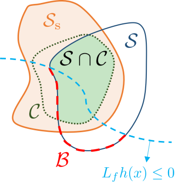
Figure 1: Visual representation of ${\mathcal{S}}_{\rm s},{\mathcal{C}},{\mathcal{S}},{\mathcal{B}}$. The set ${\mathcal{S}}\cap{\mathcal{C}}$ is control forward invariant with respect to (2) under the conditions outlined in Proposition 2. Furthermore, a relaxed set of assumptions is provided in Remark 1.

Next, define

$${\mathcal{B}}\triangleq\{x\in\mbox{bd }{\mathcal{S}}\colon L_{f}h(x)\leq 0\},$$ (12)

and note that if for all $x\in{\mathcal{B}}$, $L_{g}h(x)\neq 0$, then $h$ is a CBF. The next results show that if $h$ is a CBF, then not only is ${\mathcal{S}}$ control forward invariant but so is ${\mathcal{S}}\cap{\mathcal{C}}$. This fact is significant because ${\mathcal{S}}\cap{\mathcal{C}}$ is a subset of ${\mathcal{S}}_{\rm s}$.

Proposition 2.

Consider (2), where (A1) is satisfied. Assume that $h^{\prime}$ is locally Lipschitz on ${\mathcal{S}}$, and for all $x\in{\mathcal{B}}$, $L_{g}h(x)\neq 0$. Then, ${\mathcal{S}}\cap{\mathcal{C}}$ is control forward invariant.

Proof.

Let $u\colon{\mathcal{S}}\to{\mathbb{R}}^{m}$ be locally Lipschitz on ${\mathcal{S}}$ such that for all $x\in\mbox{bd }{\mathcal{S}}$, $L_{f}h(x)+L_{g}h(x)u(x)\geq 0$, which exists because $f$, $g$, and $h^{\prime}$ are locally Lipschtiz on ${\mathcal{S}}$ and for all $x\in{\mathcal{B}}$, $L_{g}h(x)\neq 0$. Thus, Nagumo’s Theorem [36, Theorem 4.7] implies that ${\mathcal{S}}$ is forward invariant with respect to (2).

Next, let $x_{0}\in{\mathcal{S}}\cap{\mathcal{C}}$. Since $x_{0}\in{\mathcal{S}}$ and ${\mathcal{S}}$ is forward invariant, it follows that for all $t\in I(x_{0})$, $h(x(t))\geq 0$. Thus, (11), Proposition 1, and (7) imply that for all $t\in I(x_{0})$, $b_{j,d_{j}-1}(x(t))\geq 0$. Since, in addition, $x_{0}\in{\mathcal{C}}_{j}\subset{\mathcal{S}}\cap{\mathcal{C}}$, it follows from Lemma 1 that for all $t\in I(x_{0})$, $x(t)\in{\mathcal{C}}_{j}$. Thus, for all $t\in I(x_{0})$, $x(t)\in{\mathcal{C}}$, which implies that for all $t\in I(x_{0})$, $x(t)\in{\mathcal{S}}\cap{\mathcal{C}}$. ∎

Remark 1.

Proposition 2 provides a sufficient condition such that $\mathcal{S}\cap\mathcal{C}$ is control forward invariant. However, Figure 1 illustrates that it is not necessary that $L_{g}h(x)\neq 0$ for all $x\in{\mathcal{B}}$. Specifically, it suffices to require that for all $x\in{\mathcal{B}}\cap{\mathcal{C}}$, $L_{g}h(x)\neq 0$.

V Closed-Form Optimal and Safe Control

This section uses the composite soft-minimum CBF (10) to construct a closed-form optimal control that guarantees safety. Specifically, we design a control that minimizes $J(x(t),u(x(t)))$ subject to the constraint that $x(t)\in{\mathcal{S}}\cap{\mathcal{C}}\subset{\mathcal{S}}_{\rm s}$.

Let $\gamma>0$, and let $\alpha:{\mathbb{R}}\to{\mathbb{R}}$ be a locally Lipschitz nondecreasing function such that $\alpha(0)=0$. For all $x\in{\mathbb{R}}^{n}$, consider the control given by

$$\Big{(}u(x),\mu(x)\Big{)}\triangleq\underset{{\tilde{u}\in{\mathbb{R}}^{m},\,\tilde{\mu}\in{\mathbb{R}}}}{\mbox{argmin}}\,J(x,\tilde{u})+\frac{1}{2}\gamma\tilde{\mu}^{2}$$ (13a)

subject to

$$L_{f}h(x)+L_{g}h(x)\tilde{u}+\alpha(h(x))+\tilde{\mu}h(x)\geq 0.$$ (13b)

The next result shows that if for all $x\in{\mathcal{B}}$, $L_{g}h(x)\neq 0$, then the quadratic program (13) is feasible.

Proposition 3.

The following statements hold:

1. Let $x\in{\mathbb{R}}^{n}\setminus{\mathcal{S}}$. Then, there exists $\tilde{u}\in{\mathbb{R}}^{m}$ and $\tilde{\mu}\in{\mathbb{R}}$ such that (13b) is satisfied.

2. Let $x\in{\mathcal{S}}\setminus{\mathcal{B}}$. Then, there exists $\tilde{u}\in{\mathbb{R}}^{m}$ and $\tilde{\mu}\geq 0$ such that (13b) is satisfied.

3. Let $x\in{\mathcal{B}}$. If $L_{g}h(x)\neq 0$, then there exists $\tilde{u}\in{\mathbb{R}}^{m}$ and $\tilde{\mu}\geq 0$ such that (13b) is satisfied.

Proof.

To prove (a), let $x_{1}\in{\mathbb{R}}^{n}\setminus{\mathcal{S}}$, which implies that $h(x_{1})<0$. Thus, $\tilde{u}=0$ and $\tilde{\mu}=-[L_{f}h(x_{1})+\alpha(h(x_{1}))]/h(x_{1})$ satisfy (13b).

To prove (b), let $x_{2}\in(\mbox{bd }{\mathcal{S}})\setminus{\mathcal{B}}$, which implies that $h(x_{2})=0$ and $L_{f}h(x_{2})>0$. Thus, $\tilde{u}=0$ and $\tilde{\mu}=0$ satisfy (13b). Next, let $x_{3}\in\mbox{int }{\mathcal{S}}$, which implies that $h(x_{3})>0$. Thus, $\tilde{u}=0$ and $\tilde{\mu}=\max\{-[L_{f}h(x_{3})+\alpha(h(x_{3}))]/{h(x_{3})},0\}\geq 0$ satisfy (13b).

To prove (c), let $x_{4}\in{\mathcal{B}}$, which implies that $h(x_{4})=0$. Since $L_{g}h(x_{4})\neq 0$, it follows that $\tilde{u}=-L_{f}h(x_{4})/L_{g}h(x_{4})$ and $\tilde{\mu}=0$ satisfy (13b). ∎

Next, consider $\omega:{\mathbb{R}}^{n}\to{\mathbb{R}}$ defined by

$$\omega(x)\triangleq L_{f}h(x)-L_{g}h(x)Q(x)^{-1}c(x)+\alpha(h(x)),$$ (14)

and define

$$\Omega\triangleq\{x\in{\mathbb{R}}^{n}:\omega(x)<0\}.$$ (15)

The following result provides a closed-form solution for the unique global minimizer $(u(x),\mu(x))$ of the constrained optimization (13). This result also shows that if $h^{\prime}$ is locally Lipschitz, then $u$ and $\mu$ are locally Lipschitz.

Theorem 1.

Assume that for all $x\in{\mathcal{B}}$, $L_{g}h(x)\neq 0$. Then, the following hold:

1. For all $x\in{\mathbb{R}}^{n}$,

   $$u(x) =-Q(x)^{-1}\mathopen{}\mathclose{{}\left(c(x)-L_{g}h(x)^{\rm T}\lambda(x)}\right),$$ (16)

   $$\mu(x) =\frac{h(x)\lambda(x)}{\gamma},$$ (17)

   where $\lambda\colon{\mathbb{R}}^{n}\to{\mathbb{R}}$ is defined by

   $$\lambda(x)\triangleq\begin{cases}\frac{-\omega(x)}{d(x)},&x\in\Omega,\\ 0,&x\notin\Omega,\\ \end{cases}$$ (18)

   and $d\colon\Omega\to{\mathbb{R}}$ is defined by

   $$d(x)\triangleq L_{g}h(x)Q(x)^{-1}L_{g}h(x)^{\rm T}+\gamma^{-1}h(x)^{2}.$$ (19)

2. For all $x\in{\mathbb{R}}^{n}$, $\lambda(x)\geq 0$, and for all $x\in{\mathcal{S}}$, $\mu(x)\geq 0$.

3. $u$, $\mu$, and $\lambda$ are continuous of ${\mathbb{R}}^{n}$.

4. Let ${\mathcal{D}}\subseteq{\mathbb{R}}^{n}$, and assume that $h^{\prime}$ is locally Lipschitz on ${\mathcal{D}}$. Then, $u$, $\mu$, and $\lambda$ are locally Lipschitz on ${\mathcal{D}}$.

Proof.

First, we show that for all $x\in\mbox{cl }\Omega$, $d(x)>0$. Let $a\in\mbox{cl }\Omega$, and assume for contradiction that $d(a)=0$. Since $\gamma>0$ and $Q$ is positive definite, it follows from (19) that $L_{g}h(a)=0$ and $h(a)=0$. Since, in addition, for all $x\in{\mathcal{B}}$, $L_{g}h(x)\neq 0$, it follows from (12) that $L_{f}h(a)>0$. Thus, (14) implies $\omega(a)=L_{f}h(a)>0$, which implies $a\notin\mbox{cl }\Omega$, which is a contradiction. Thus, $d(a)\not=0$, which implies that $d(a)>0$. Thus, for all $x\in\mbox{cl }\Omega$, $d(x)>0$.

To prove 19, define

$$\tilde{J}(x,\tilde{u},\tilde{\mu})\triangleq J(x,\tilde{u})+\frac{1}{2}\gamma\tilde{\mu}^{2},$$

$$b(x,\tilde{u},\tilde{\mu})\triangleq L_{f}h(x)+L_{g}h(x)\tilde{u}+\alpha(h(x))+\tilde{\mu}h(x),$$

$$u_{*}(x)\triangleq-Q(x)^{-1}c(x),$$

and note that $u_{*}$ is the unique global minimizer of $J$, which implies that $(u_{*},0)$ is the unique global minimizer of $\tilde{J}$.

First, let $x_{1}\notin\Omega$, and it follows from (15) that $\omega(x_{1})\geq 0$, which combined with (14) implies that $(\tilde{u},\tilde{\mu})=(u_{*}(x_{1}),0)$ satisfies (13b). Since, in addition, $(\tilde{u},\tilde{\mu})=(u_{*}(x_{1}),0)$ is the unique global minimizer of $\tilde{J}(x_{1},\tilde{u},\tilde{\mu})$, it follows that $(\tilde{u},\tilde{\mu})=(u_{*}(x_{1}),0)$ is the solution to (13). Finally, 16, 17, 18, and 19 yields $u(x_{1})=u_{*}(x_{1})$ and $\mu(x_{1})=0$, which confirms 19 for all $x\notin\Omega$.

Next, let $x_{2}\in\Omega$. Let $(u_{2},\mu_{2})\in{\mathbb{R}}^{m}\times{\mathbb{R}}$ denote the the unique global minimizer of $\tilde{J}(x_{2},\tilde{u},\tilde{\mu})$ subject to $b(x_{2},\tilde{u},\tilde{\mu})\geq 0$. Since $x_{2}\in\Omega$, it follows from (14) that $b(x_{2},u_{*}(x_{2}),0)=\omega(x_{2})<0$. Thus, $b(x_{2},u_{2},\mu_{2})=0$. Define the Lagrangian

$${\mathcal{L}}(\tilde{u},\tilde{\mu},\tilde{\lambda})\triangleq\tilde{J}(x_{2},\tilde{u},\tilde{\mu})-\tilde{\lambda}b(x_{2},\tilde{u},\tilde{\mu}).$$

Let $\lambda_{2}\in{\mathbb{R}}$ be such that $(u_{2},\mu_{2},\lambda_{2})$ is a stationary point of ${\mathcal{L}}$. Evaluating $\frac{\partial{\mathcal{L}}}{\partial{\tilde{u}}}$, $\frac{\partial{\mathcal{L}}}{\partial\tilde{\mu}}$, and $\frac{\partial{\mathcal{L}}}{\partial\tilde{\lambda}}$ at $(u_{2},\mu_{2},\lambda_{2})$; setting equal to zero; and solving for $u_{2}$, $\mu_{2}$, and $\lambda_{2}$ yields

$$u_{2}=-Q(x_{2})^{-1}\mathopen{}\mathclose{{}\left(c(x_{2})-L_{g}h(x_{2})^{\rm T}\lambda_{2}}\right),$$

$$\mu_{2}=\frac{h(x_{2})\lambda_{2}}{\gamma},$$

$$\lambda_{2}=\frac{-\omega(x_{2})}{d(x_{2})},$$

where $d(x_{2})\neq 0$ because $x_{2}\in\Omega$. Finally, 16, 17, 18, and 19 yields $u(x_{2})=u_{2}$, $\mu(x_{2})=\mu_{2}$, and $\lambda(x_{2})=\lambda_{2}$, which confirms 19 for all $x\in\Omega$.

To prove (b), since $d$ is positive on $\mbox{cl }\Omega$, it follows from 14, 15, and 18 that for all $x\in{\mathbb{R}}^{n}$, $\lambda(x)\geq 0$. Since, in addition, $\gamma>0$ and $h$ is nonnegative on ${\mathcal{S}}$, it follows from 17 that for all $x\in{\mathcal{S}}$, $\mu(x)\geq 0$.

To prove (c), let $a\in\mbox{bd }\Omega$, which implies that $\omega(a)=0$ and $d(a)>0$. Thus, $-\omega(a)/d(a)=0$, and (18) implies that $\lambda$ is continuous on $\mbox{bd }\Omega$. Since, in addition, $f$, $g$, $Q^{-1}$, $c$, $h$, and $h^{\prime}$ are continuous on ${\mathbb{R}}^{n}$, it follows from 14, 18, and 19 that $\lambda$ is continuous on ${\mathbb{R}}^{n}$, which combined with (16) and (17) implies that $u$ and $\mu$ are continuous on ${\mathbb{R}}^{n}$.

To prove (d), note that $f$, $g$, $Q^{-1}$, $c$, $\alpha$ and $h$ are locally Lipschitz on ${\mathbb{R}}^{n}$. Since $h^{\prime}$ is locally Lipschitz on ${\mathcal{D}}$, it follows from 14 and 19 that $\omega$ and $d$ are locally Lipschitz on ${\mathcal{D}}$. Thus, 18 implies that $\lambda$ is locally Lipschitz on ${\mathcal{D}}$, which combined with 16 and 17 implies that $u$ and $\mu$ are locally Lipschitz on ${\mathcal{D}}$. ∎

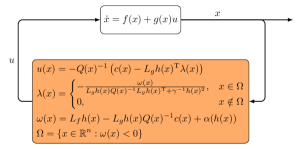
Figure 2: Closed-form optimal and safe control using the composite soft-minimum CBF (10). Control minimizes cost $J$ subject to safety constraint.

Figure 2 is a block diagram of the control 6, 10, 16, 14, 15, 17, 18, and 19, which is the closed-form solution to the quadratic program (13) that relies on the composite soft-minimum CBF $h$. The next theorem is the main result on safety using this control.

Theorem 2.

Consider (2), where (A1) is satisfied, and consider $u$ given by 6, 10, 16, 14, 15, 17, 18, and 19. Assume that $h^{\prime}$ is locally Lipschitz on ${\mathcal{S}}$, and for all $x\in{\mathcal{B}}$, $L_{g}h(x)\neq 0$. Let $x_{0}\in{\mathcal{S}}\cap{\mathcal{C}}$. Then, for all $t\in I(x_{0})$, $x(t)\in{\mathcal{S}}\cap{\mathcal{C}}\subset{\mathcal{S}}_{\rm s}$.

Proof.

Since $h^{\prime}$ is locally Lipschitz on ${\mathcal{S}}$, it follows from (d) of Theorem 1 that $u$ is locally Lipschitz on ${\mathcal{S}}$. Next, let $a\in\mbox{bd }{\mathcal{S}}$, which implies that $h(a)=0$. Thus, 16, 14, 15, 17, 18, and 19 imply that

$$L_{f}h(a)+L_{g}h(a)u(a) =L_{f}h(a)-L_{g}h(a)Q(a)^{-1}c(a)$$

$$\quad+L_{g}h(a)Q(a)^{-1}L_{g}h(a)^{\rm T}\lambda(a)$$

$$=\begin{cases}0,&a\in\Omega\\ \omega(a),&a\notin\Omega\end{cases}$$

$$\geq 0.$$

Hence, for all $x\in\mbox{bd }{\mathcal{S}}$, $L_{f}h(x)+L_{g}h(x)u(x)\geq 0$. Thus, [36, Theorem 4.7] implies that ${\mathcal{S}}$ is forward invariant with respect to (2).

Next, let $x_{0}\in{\mathcal{S}}\cap{\mathcal{C}}$. Since $x_{0}\in{\mathcal{S}}$ and ${\mathcal{S}}$ is forward invariant, it follows that for all $t\in I(x_{0})$, $h(x(t))\geq 0$. Thus, (11), Proposition 1, and (7) imply that for all $t\in I(x_{0})$, $b_{j,d_{j}-1}(x(t))\geq 0$. Since, in addition, $x_{0}\in{\mathcal{C}}_{j}\subset{\mathcal{S}}\cap{\mathcal{C}}$, it follows from Lemma 1 that for all $t\in I(x_{0})$, $x(t)\in{\mathcal{C}}_{j}$. Thus, for all $t\in I(x_{0})$, $x(t)\in{\mathcal{C}}$, which implies that for all $t\in I(x_{0})$, $x(t)\in{\mathcal{S}}\cap{\mathcal{C}}$. ∎

The control 6, 10, 16, 14, 15, 17, 18, and 19 relies on the Lie derivatives $L_{f}h$ and $L_{g}h$, which can be expressed as

$$L_{f}h(x) =\sum_{j=1}^{\ell}\beta_{j}(x)L_{f}b_{j,d_{j}-1}(x),$$

$$=\sum_{j=1}^{\ell}\beta_{j}(x)\Big{[}L_{f}^{d_{j}}h_{j}(x)$$

$$\qquad+\sum_{k=0}^{d_{j}-2}L_{f}^{k+1}\alpha_{j,d_{j}-2-k}\mathopen{}\mathclose{{}\left(b_{j,d_{j}-2-k}(x)}\right)\Big{]},$$

$$L_{g}h(x) =\sum_{j=1}^{\ell}\beta_{j}(x)L_{g}b_{j,d_{j}-1}(x)$$

$$=\sum_{j=1}^{\ell}\beta_{j}(x)L_{g}L_{f}^{d_{j}-1}h_{j}(x),$$

where

$$\beta_{j}(x)\triangleq\exp\rho(h(x)-b_{j,d_{j}-1}(x)).$$

It follows from 1 and 10 that $\sum_{j=1}^{\ell}\beta_{j}(x)=1$, which implies that for each $x\in{\mathbb{R}}^{n}$, $L_{f}h(x)$ and $L_{g}h(x)$ are convex combinations of $L_{f}b_{1,d_{1}-1}(x),\ldots,L_{f}b_{\ell,d_{\ell}-1}(x)$ and $L_{g}b_{1,d_{1}-1}(x),\ldots,L_{g}b_{\ell,d_{\ell}-1}(x)$, respectively. The next result follows from this observation and provides a sufficient condition such that for all $x\in{\mathcal{B}}$, $L_{g}h(x)\neq 0$.

Proposition 4.

Assume (A1) is satisfied, and assume for all $x\in{\mathcal{B}}$, $0\not\in\mbox{conv}\{L_{g}L_{f}^{d_{1}-1}h_{1}(x),\ldots,L_{g}L_{f}^{d_{\ell}-1}h_{\ell}(x)\}$. Then, for all $x\in{\mathcal{B}}$, $L_{g}h(x)\neq 0$.

Proposition 4 provides a sufficient condition such that $L_{g}h(x)\neq 0$ for all $x\in{\mathcal{B}}$. However, this condition is not necessary.

Next, we present an example to demonstrate the control 6, 10, 16, 14, 15, 17, 18, and 19.

Example 1.

Consider the nonholonomic ground robot modeled by (2), where

$$f(x)=\begin{bmatrix}v\cos{\theta}\\ v\sin{\theta}\\ 0\\ 0\end{bmatrix},\,g(x)=\begin{bmatrix}0&0\\ 0&0\\ 1&0\\ 0&1\end{bmatrix},\,x=\begin{bmatrix}q_{\rm x}\\ q_{\rm y}\\ v\\ \theta\end{bmatrix},\,u=\begin{bmatrix}u_{1}\\ u_{2}\end{bmatrix},$$

and $q\triangleq[\,q_{\rm x}\quad q_{\rm y}\,]^{\rm T}$ is the robot’s position in an orthogonal coordinate system, $v$ is the speed, and $\theta$ is the direction of the velocity vector (i.e., the angle from $[\,1\quad 0\,]^{\rm T}$ to $[\,\dot{q}_{\rm x}\quad\dot{q}_{\rm y}\,]^{\rm T}$).

Consider the map shown in Figure 3, which has 6 obstacles and a wall. For $j\in\{1,\ldots,6\}$, the area outside the $j$th obstacle is modeled as the zero-superlevel set of

$$h_{j}(x)=\mathopen{}\mathclose{{}\left\|\mathopen{}\mathclose{{}\left[\begin{smallmatrix}a_{{\rm x},j}(q_{\rm x}-b_{{\rm x},j})\\ a_{{\rm y},j}(q_{\rm y}-b_{{\rm y},j})\end{smallmatrix}}\right]}\right\|_{p}-c_{j},$$ (20)

where $b_{{\rm x},j},b_{{\rm y},j},a_{{\rm x},j},a_{{\rm y},j},c_{j},p>0$ specify the location and dimensions of the $j$th obstacle. Similarly, the area inside the wall is modeled as the zero-superlevel set of

$$h_{7}(x)=c_{7}-\mathopen{}\mathclose{{}\left\|\mathopen{}\mathclose{{}\left[\begin{smallmatrix}a_{{\rm x},7}q_{\rm x}\\ a_{{\rm y},7}q_{\rm y}\end{smallmatrix}}\right]}\right\|_{p},$$ (21)

where $a_{{\rm x},7},a_{{\rm y},7},c_{7},p>0$ specify the dimension of the space inside the wall. The bounds on speed $v$ are modeled as the zero-superlevel sets of

$$h_{8}(x)=9-v,\qquad h_{9}(x)=v+1.$$ (22)

The safe set ${\mathcal{S}}_{\rm s}$ is given by (4) where $\ell=9$. The projection of ${\mathcal{S}}_{\rm s}$ onto the $q_{\rm x}$–$q_{\rm y}$ plane is shown in Figure 3. Note that for all $x\in{\mathcal{S}}_{\rm s}$, the speed satisfies $v\in[-1,9]$. We also note that (A1) is satisfied with $d_{1}=d_{2}=\ldots=d_{7}=2$ and $d_{8}=d_{9}=1$.

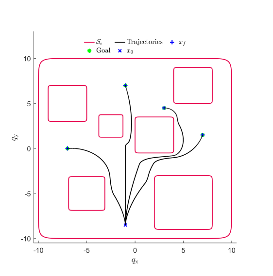
Figure 3: Safe set ${\mathcal{S}}_{\rm s}$, and closed-loop trajectories for 4 goal locations.

Let $q_{{\rm d}}=[\,q_{{\rm d},{\rm x}}\quad q_{{\rm d},{\rm y}}\,]^{\rm T}\in{\mathbb{R}}^{2}$ be the goal location, that is, the desired location for $q$. Then, consider the desired control

$$u_{\rm d}(x)\triangleq\begin{bmatrix}u_{{\rm d}_{1}}(x)\\ u_{{\rm d}_{2}}(x)\end{bmatrix},$$ (23)

where $u_{{\rm d}_{1}},u_{{\rm d}_{2}},\psi:{\mathbb{R}}^{4}\to{\mathbb{R}}$ are

$$u_{{\rm d}_{1}}(x) \triangleq-(k_{1}+k_{3})v+(1+k_{1}k_{3})\|q-q_{\rm d}\|_{2}\cos\psi(x)$$

$$\qquad+k_{1}\mathopen{}\mathclose{{}\left(k_{2}\|q-q_{\rm d}\|_{2}+v}\right)\sin^{2}\psi(x),$$ (24)

$$u_{{\rm d}_{2}}(x) \triangleq\mathopen{}\mathclose{{}\left(k_{2}+\frac{v}{\|q-q_{\rm d}\|_{2}}}\right)\sin\psi(x),$$ (25)

$$\psi(x) \triangleq\mbox{atan2}(q_{\rm y}-q_{{\rm d},{\rm y}},q_{\rm x}-q_{{\rm d},{\rm x}})-\theta+\pi,$$ (26)

and $k_{1}=0.2,k_{2}=1$, and $k_{3}=2$. Note that the desired control is designed using a process similar to [37, pp. 30–31], and it drives $[\,q_{\rm x}\quad q_{\rm y}\,]^{\rm T}$ to $q_{\rm d}$ but does not account for safety.

We consider the cost (5), where $Q(x)=I_{2}$ and $c(x)=-u_{\rm d}(x)$. Thus, the minimizer of (5) is equal to the minimizer of the minimum-intervention cost $\|u-u_{\rm d}(x)\|_{2}^{2}$.

We implement the control 6, 10, 16, 14, 15, 17, 18, and 19 with $\rho=10$, $\gamma=10^{24}$, $\alpha_{1,0}(h)=\ldots=\alpha_{7,0}(h)=7h$, and $\alpha(h)=0.5h$. The control is updated at $1~{}\rm{kHz}$.

Figure 3 shows the closed-loop trajectories for $x_{0}=[\,-1\quad-8.5\quad 0\quad{\pi}/{2}\,]^{\rm T}$ and 4 different goal locations: $q_{{\rm d}}=[\,3\quad 4.5\,]^{\rm T}$, $q_{{\rm d}}=[\,-7\quad 0\,]^{\rm T}$, $q_{{\rm d}}=[\,7\quad 1.5\,]^{\rm T}$, and $q_{{\rm d}}=[\,-1\quad 7\,]^{\rm T}$. In all cases, the robot position converges to the goal location while satisfying the safety constraints.

Figures 4 and 5 show the trajectories of the relevant signals for the case where $q_{{\rm d}}=[\,3\quad 4.5\,]^{\rm T}$. Figures 4 shows that the robot position converges to the goal location and that the control is equal to the desired control except for $t\in[0.3,0.9]\cup[1.5,2.9]\cup[5,5.6]$. Figure 5 shows that $h$, $\min b_{j,i}$, and $\min h_{j}$ are positive for all time, which implies trajectory remains in ${\mathcal{S}}\cap{\mathcal{C}}\subset{\mathcal{S}}_{\rm s}$.  $\triangle$

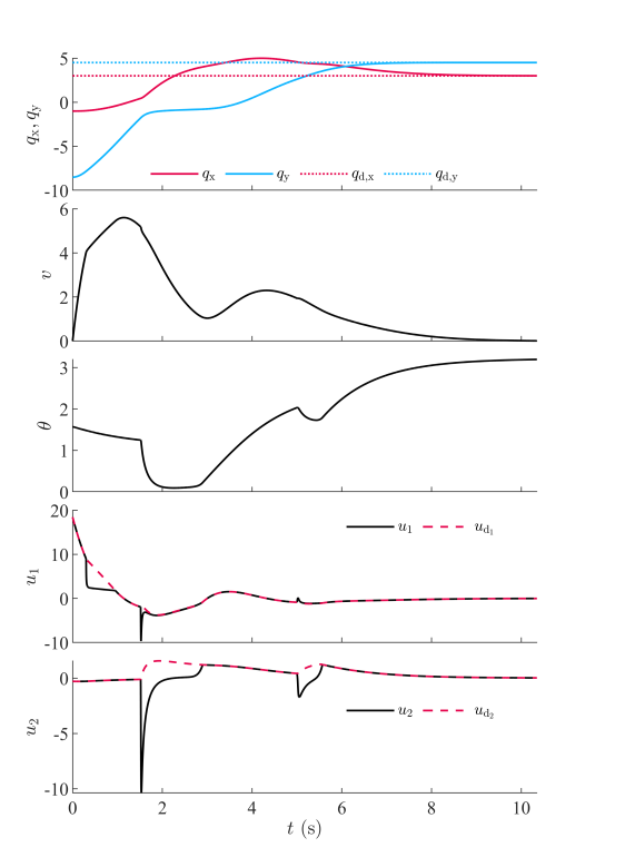
Figure 4: $q_{\rm x}$, $q_{\rm y}$, $v$, $\theta$, $u$ and $u_{\rm d}$ for $q_{{\rm d}}=[\,3\quad 4.5\,]^{\rm T}$.

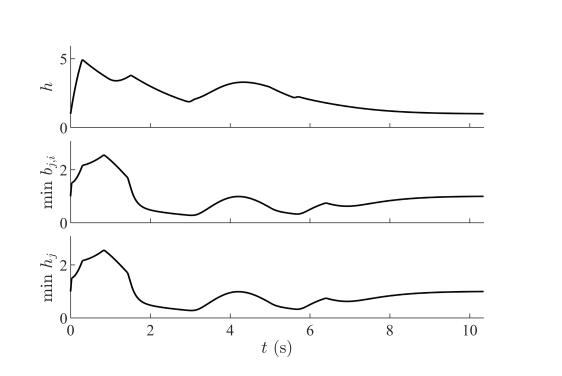
Figure 5: $h$, $\min b_{j,i}$, and $\min h_{j}$ for $q_{{\rm d}}=[\,3\quad 4.5\,]^{\rm T}$.

VI Safety with Input Constraints

This section extends the approach of Section V to guarantee safety subject to input constraints (e.g., actuator limits). Specifically, we use the composite soft-minimum CBF (10) to construct a closed-form optimal control that not only guarantees safety but also respects specified input constraints.

We reconsider the system (2), safe set (4), and cost (5). Next, let $\phi_{1},\ldots,\phi_{\ell_{u}}:{\mathbb{R}}^{m}\to{\mathbb{R}}$ be continuously differentiable, and define the set of admissible controls

$${\mathcal{U}}\triangleq\{u\in{\mathbb{R}}^{m}:\phi_{1}(u)\geq 0,\ldots,\phi_{\ell_{u}}(u)\geq 0\}\subseteq{\mathbb{R}}^{m}.$$ (27)

We assume that for all $u\in{\mathcal{U}}$ and all $\kappa\in\{1,2,\ldots,\ell_{u}\}$, $\phi^{\prime}_{\kappa}(u)\neq 0$.

The objective is to design a full-state feedback control such that for all $t\geq 0$, $J(x(t),u(t))$ is minimized subject to the safety constraint that $x(t)\in{\mathcal{S}}_{\rm s}$ and the input constraint that $u(t)\in{\mathcal{U}}$.

VI-A Control Dynamics to Transform Input Constraints into Controller State Constraints

To address safety with input constraints, we introduce control dynamics. Specifically, consider the control $u$ that satisfies

$$\dot{x}_{\rm c}(t) =f_{\rm c}(x_{\rm c}(t))+g_{\rm c}(x_{\rm c}(t))\hat{u}(x(t),x_{\rm c}(t)),$$ (28)

$$u(t) =h_{\rm c}(x_{\rm c}(t)),$$ (29)

where $x_{\rm c}(t)\in{\mathbb{R}}^{n_{\rm c}}$ is the controller state; $x_{\rm c}(0)=x_{{\rm c}0}\in{\mathbb{R}}^{n_{\rm c}}$ is the initial condition; $f_{\rm c}:{\mathbb{R}}^{n_{\rm c}}\to{\mathbb{R}}^{n_{\rm c}}$, $g_{\rm c}:{\mathbb{R}}^{n_{\rm c}}\to{\mathbb{R}}^{{n_{\rm c}}\times m}$, and $h_{\rm c}:{\mathbb{R}}^{n_{\rm c}}\to{\mathbb{R}}^{m}$ are locally Lipschitz on ${\mathbb{R}}^{n_{\rm c}}$; and $\hat{u}:{\mathbb{R}}^{n+n_{\rm c}}\to{\mathbb{R}}^{m}$ is given by the closed-form solution to a quadratic program presented later in this section.

Define

$${\mathcal{S}}_{{\rm c}}\triangleq\{x_{\rm c}\in{\mathbb{R}}^{n_{\rm c}}:h_{\rm c}(x_{\rm c})\in{\mathcal{U}}\},$$ (30)

which is the set of controller states such that the control is in the set of admissible controls ${\mathcal{U}}$. Thus, using the control dynamics 28 and 29 transformed the input constraint (i.e., $u(t)\in{\mathcal{U}}$) into a constraint on the state of the controller (i.e., $x_{\rm c}(t)\in{\mathcal{S}}_{\rm c}$).

Next, consider the cascade of 2, 28, and 29, which is given by

$$\dot{\hat{x}}=\hat{f}(\hat{x})+\hat{g}(\hat{x})\hat{u},$$ (31)

where

$$\qquad\hat{x}\triangleq\begin{bmatrix}x\\ x_{\rm c}\end{bmatrix},\qquad\hat{f}(\hat{x})\triangleq\begin{bmatrix}f(x)+g(x)h_{\rm c}(x_{\rm c})\\ f_{\rm c}(x_{\rm c})\end{bmatrix},$$ (32)

$$\hat{g}(\hat{x})\triangleq\begin{bmatrix}0\\ g_{\rm c}(x_{\rm c})\end{bmatrix},\qquad\hat{x}_{0}\triangleq\begin{bmatrix}x_{0}\\ x_{{\rm c}0}\end{bmatrix},$$ (33)

and $\hat{n}\triangleq n+n_{\rm c}$. Define

$$\hat{\mathcal{S}}_{\rm s}\triangleq{\mathcal{S}}_{\rm s}\times{\mathcal{S}}_{{\rm c}},$$ (34)

which is the set of cascade states $\hat{x}$ such that the safety constraint (i.e., $x(t)\in{\mathcal{S}}_{\rm s}$) and the input constraint (i.e., $u(t)\in{\mathcal{U}}$) are satisfied. The next result summarizes this property.

Proposition 5.

Assume that for all $t\geq 0$, $\hat{x}(t)\in\hat{\mathcal{S}}_{\rm s}$. Then, for all $t\geq 0$, $x(t)\in{\mathcal{S}}_{\rm s}$ and $u(t)\in{\mathcal{U}}$.

Proof.

Let $t_{1}\geq 0$. Since $\hat{x}(t_{1})\in\hat{\mathcal{S}}_{\rm s}$, it follows from (34) that $x(t_{1})\in{\mathcal{S}}_{\rm s}$ and $x_{\rm c}(t_{1})\in{\mathcal{S}}_{\rm c}$. Since $x_{\rm c}(t_{1})\in{\mathcal{S}}_{\rm c}$, it follows from 29 and 30 that $u(t_{1})\in{\mathcal{U}}$. ∎

The functions $f_{\rm c}$, $g_{\rm c}$ and $h_{\rm c}$ are selected such that the following conditions hold:

1. There exists a positive integer $d_{\rm c}$ such that for all $x_{\rm c}\in{\mathcal{S}}_{{\rm c}}$, $L_{g_{\rm c}}h_{\rm c}(x_{\rm c})=L_{g_{\rm c}}L_{f_{\rm c}}h_{\rm c}(x_{\rm c})=\cdots=L_{g_{\rm c}}L_{f_{\rm c}}^{d_{\rm c}-2}h_{\rm c}(x_{\rm c})=0$ and $L_{g_{\rm c}}L_{f_{\rm c}}^{d_{\rm c}-1}h_{\rm c}(x_{\rm c})$ is nonsingular.

2. There exists a positive integer $\zeta$ such that for all $\kappa\in\{1,2,\ldots,\ell_{u}\}$ and all $x_{\rm c}\in{\mathcal{S}}_{{\rm c}}$, $L_{g_{\rm c}}\phi_{\kappa}(h_{\rm c}(x_{\rm c}))=L_{g_{\rm c}}L_{f_{\rm c}}\phi_{\kappa}(h_{\rm c}(x_{\rm c}))=\cdots=L_{g_{\rm c}}L_{f_{\rm c}}^{\zeta-2}\phi_{\kappa}(h_{\rm c}(x_{\rm c}))=0$ and $L_{g_{\rm c}}L_{f_{\rm c}}^{\zeta-1}\phi_{\kappa}(h_{\rm c}(x_{\rm c}))\neq 0$.

Note that $f_{\rm c}$, $g_{\rm c}$, and $h_{\rm c}$ can be designed such that (C1) and (C2) are satisfied. The following example provides one construction of $f_{\rm c}$, $g_{\rm c}$, and $h_{\rm c}$ such that (C1) and (C2) are satisfied. In particular, this example provides a linear time-invariant controller such that (C1) and (C2) are satisfied.

Example 2.

Let

$$f_{\rm c}(x_{\rm c})=A_{\rm c}x_{\rm c},\quad g_{\rm c}(x_{\rm c})=B_{\rm c},\quad h_{\rm c}(x_{\rm c})=C_{\rm c}x_{\rm c},$$

where $A_{\rm c}\in{\mathbb{R}}^{n_{\rm c}\times n_{\rm c}}$, $B_{\rm c}\in{\mathbb{R}}^{n_{\rm c}\times m}$, $C_{\rm c}\in{\mathbb{R}}^{m\times n_{\rm c}}$, and $C_{\rm c}B_{\rm c}$ is nonsingular.

First, note that $L_{g_{\rm c}}h_{\rm c}(x_{\rm c})=C_{\rm c}B_{\rm c}$. Since $C_{\rm c}B_{\rm c}$ is nonsingular, it follows that (C1) is satisfied with $d_{\rm c}=1$. Next, note that $L_{g_{\rm c}}\phi_{\kappa}(h_{\rm c}(x_{\rm c}))=\phi_{\kappa}^{\prime}(h_{\rm c}(x_{\rm c}))C_{\rm c}B_{\rm c}$. Since $C_{\rm c}B_{\rm c}$ is nonsingular and for all $x_{\rm c}\in{\mathcal{S}}_{\rm c}$, $\phi_{\kappa}^{\prime}(h_{\rm c}(x_{\rm c}))\neq 0$, it follows that (C2) is satisfied with $\zeta=1$. Thus, any linear time-invariant controller with $C_{\rm c}B_{\rm c}$ is nonsingular satisfies (C1) and (C2). For example, we could let $a>0$, $A_{\rm c}=-aI_{n_{\rm c}}$, $B_{\rm c}=I_{n_{\rm c}}$, and $C_{\rm c}=I_{n_{\rm c}}$, which implies that the controller is low pass.  $\triangle$

Next, let $\hat{\ell}\triangleq\ell+\ell_{u}$. Unless otherwise stated, all statements in this section that involve the subscript $\hat{\jmath}$ are for all $\hat{\jmath}\in\{1,2,\ldots,\hat{\ell}\}$. Let $\hat{h}_{\hat{\jmath}}\colon{\mathbb{R}}^{\hat{n}}\to{\mathbb{R}}$ be defined by

$$\hat{h}_{\hat{\jmath}}(\hat{x})\triangleq\begin{cases}h_{\hat{\jmath}}(x),&\mbox{if }{\hat{\jmath}}\in\{1,2,\ldots,\ell\},\\ \phi_{{\hat{\jmath}}-\ell}(h_{\rm c}(x_{\rm c})),&\mbox{if }{\hat{\jmath}}\in\{\ell+1,\ell+2,\ldots,\ell+\ell_{u}\},\end{cases}$$ (35)

and define

$$\hat{d}_{\hat{\jmath}}\triangleq\begin{cases}d_{\hat{\jmath}}+d_{\rm c},&\mbox{if }{\hat{\jmath}}\in\{1,2,\ldots,\ell\},\\ \zeta,&\mbox{if }{\hat{\jmath}}\in\{\ell+1,\ell+2,\ldots,\ell+\ell_{u}\}.\end{cases}$$ (36)

The following result demonstrates that $\hat{h}_{\hat{\jmath}}$ has well-defined relative degree $\hat{d}_{\hat{\jmath}}$ with respect to the cascade 31, 32, and 33 on $\hat{\mathcal{S}}_{\rm s}$; however, relative degrees $\hat{d}_{1},\ldots,\hat{d}_{\hat{\ell}}$ are not all equal.

Proposition 6.

Consider (2), where (A1) is satisfied, and consider 28 and 29, where (C1) and (C2) are satisfied. Then, for all $\hat{x}\in\hat{\mathcal{S}}_{\rm s}$, $L_{\hat{g}}\hat{h}_{\hat{\jmath}}(\hat{x})=L_{\hat{g}}L_{\hat{f}}\hat{h}_{\hat{\jmath}}(\hat{x})=\cdots=L_{\hat{g}}L_{\hat{f}}^{\hat{d}_{\hat{\jmath}}-2}\hat{h}_{\hat{\jmath}}(\hat{x})=0$ and $L_{\hat{g}}L_{\hat{f}}^{\hat{d}_{\hat{\jmath}}-1}\hat{h}_{\hat{\jmath}}(\hat{x})\neq 0$.

Proof.

Let $a\in\{1,2,\ldots,\ell\}$, and it follows from (A1) and (C1) that (A2) in Appendix A is satisfied for $x_{1}$, $x_{2}$, $f_{1}$, $g_{1}$, $f_{2}$, $g_{2}$, ${\mathcal{X}}_{1}$, ${\mathcal{X}}_{2}$, $\xi_{1}$, $\xi_{2}$, $r_{1}$, $r_{2}$ equal to $x$, $x_{\rm c}$, $f$, $g$, $f_{\rm c}$, $g_{\rm c}$, ${\mathcal{S}}_{\rm s}$, ${\mathcal{S}}_{\rm c}$, $h_{a}$, $h_{\rm c}$, $d_{a}$, $d_{\rm c}$, respectively. Thus, it follows from Theorem 3 in Appendix A that $L_{\hat{g}}\hat{h}_{a}(\hat{x})=\cdots=L_{\hat{g}}L_{\hat{f}}^{d_{a}+d_{\rm c}-2}\hat{h}_{a}(\hat{x})=0$ and $L_{\hat{g}}L_{\hat{f}}^{d_{a}+d_{\rm c}-1}\hat{h}_{a}(\hat{x})=[L_{g}L_{f}^{d_{a}-1}h_{a}(x)]L_{g_{\rm c}}L_{f_{\rm c}}^{d_{\rm c}-1}h_{\rm c}(x_{\rm c})$. Since, in addition, (A1) implies that $L_{g}L_{f}^{d_{a}-1}h_{a}(x)\neq 0$ and (C1) implies that $L_{g_{\rm c}}L_{f_{\rm c}}^{d_{\rm c}-1}h_{\rm c}(x_{\rm c})$ is nonsingular, it follows that $L_{\hat{g}}L_{\hat{f}}^{d_{a}+d_{\rm c}-1}\hat{h}_{a}(\hat{x})\neq 0$, which confirms the result for $\hat{\jmath}\in\{1,2,\ldots,\ell\}$.

Let $b\in\{\ell+1,\ell+2,\ldots,\hat{\ell}\}$ and let $i\in\{0,1,\ldots\zeta-1\}$. Next, it follows from 32 that $L_{\hat{f}}^{i}\hat{h}_{b}(\hat{x})=L_{\hat{f}}^{i}\phi_{b-\ell}(h_{\rm c}(x_{\rm c}))=L_{\hat{f}}^{i-1}L_{f_{\rm c}}\phi_{b-\ell}(h_{\rm c}(x_{\rm c}))=\cdots=L^{i}_{f_{\rm c}}\phi_{b-\ell}(h_{\rm c}(x_{\rm c}))$, which combined with (33) implies that

$$L_{\hat{g}}L_{\hat{f}}^{i}\hat{h}_{b}(\hat{x})=L_{\hat{g}}L^{i}_{f_{\rm c}}\phi_{b-\ell}(h_{\rm c}(x_{\rm c}))=L_{g_{\rm c}}L^{i}_{f_{\rm c}}\phi_{b-\ell}(h_{\rm c}(x_{\rm c})).$$

Thus, (C2) implies that $L_{\hat{g}}\hat{h}_{b}(\hat{x})=\cdots=L_{\hat{g}}L_{\hat{f}}^{\zeta-2}\hat{h}_{b}(\hat{x})=0$ and $L_{\hat{g}}L_{\hat{f}}^{\zeta-1}\hat{h}_{b}(\hat{x})\neq 0$, which combined with (36) confirms the result for $\hat{\jmath}\in\{\ell+1,\ell+2,\ldots,\hat{\ell}\}$. ∎

VI-B Composite Soft-Minimum CBF

Proposition 6 implies that the cascade 31, 32, and 33 with the CBFs $\hat{h}_{1},\ldots,\hat{h}_{\hat{\ell}}$ satisfy (A1), where $f$, $g$, $x$, ${\mathcal{S}}_{\rm c}$, $\ell$, $j$, $h_{j}$, and $d_{j}$ are replaced by $\hat{f}$, $\hat{g}$, $\hat{x}$, $\hat{\mathcal{S}}_{\rm c}$, $\hat{\ell}$, $\hat{\jmath}$, $\hat{h}_{\hat{\jmath}}$, and $\hat{d}_{\hat{\jmath}}$. Thus, the composite soft-minimum CBF construction in Section IV can be applied to the cascade 31, 32, and 33 in order to construct a single CBF from the CBFs $\hat{h}_{1},\ldots,\hat{h}_{\hat{\ell}}$, which do not all have the same relative degree. Note that $\hat{h}_{1},\ldots,\hat{h}_{\hat{\ell}}$ describe the set $\hat{\mathcal{S}}_{\rm s}={\mathcal{S}}_{\rm s}\times{\mathcal{S}}_{\rm c}$ that combines the safe set ${\mathcal{S}}_{\rm s}$ and the set ${\mathcal{S}}_{\rm c}$ of controller states such that the control is in the admissible set ${\mathcal{U}}$. Thus, the composite soft-minimum CBF can be used to address both safety and the input constraints.

First, let $\hat{b}_{{\hat{\jmath}},0}(\hat{x})\triangleq\hat{h}_{\hat{\jmath}}(\hat{x})$. For $i\in\{0,1\ldots,\hat{d}_{\hat{\jmath}}-2\}$, let $\hat{\alpha}_{{\hat{\jmath}},i}\colon{\mathbb{R}}\to{\mathbb{R}}$ be a locally Lipschitz extended class-${\mathcal{K}}$ function, and consider $\hat{b}_{{\hat{\jmath}},i+1}:{\mathbb{R}}^{\hat{n}}\to{\mathbb{R}}$ defined by

$$\hat{b}_{{\hat{\jmath}},i+1}(\hat{x})\triangleq L_{\hat{f}}\hat{b}_{{\hat{\jmath}},i}(\hat{x})+\hat{\alpha}_{{\hat{\jmath}},i}(\hat{b}_{{\hat{\jmath}},i}(\hat{x})).$$ (37)

For $i\in\{0\ldots,\hat{d}_{\hat{\jmath}}-1\}$, define

$$\hat{\mathcal{C}}_{{\hat{\jmath}},i}\triangleq\{\hat{x}\in{\mathbb{R}}^{\hat{n}}\colon\hat{b}_{{\hat{\jmath}},i}(\hat{x})\geq 0\}.$$

Next, define

$$\hat{\mathcal{C}}_{\hat{\jmath}}\triangleq\begin{cases}\hat{\mathcal{C}}_{{\hat{\jmath}},0},&\hat{d}_{\hat{\jmath}}=1,\\ \bigcap_{i=0}^{\hat{d}_{\hat{\jmath}}-2}\hat{\mathcal{C}}_{{\hat{\jmath}},i},&\hat{d}_{\hat{\jmath}}>1,\end{cases}$$

and

$$\hat{\mathcal{C}}\triangleq\bigcap_{{\hat{\jmath}}=1}^{\hat{\ell}}\hat{\mathcal{C}}_{\hat{\jmath}}.$$

Let $\rho>0$, and consider $\hat{h}:{\mathbb{R}}^{\hat{n}}\to{\mathbb{R}}$ defined by

$$\hat{h}(\hat{x})\triangleq\mbox{softmin}_{\rho}\Big{(}\hat{b}_{1,\hat{d}_{1}-1}(\hat{x}),\hat{b}_{2,\hat{d}_{2}-1}(\hat{x}),\ldots,\hat{b}_{\hat{\ell},\hat{d}_{\hat{\ell}}-1}(\hat{x})\Big{)},$$ (38)

and define

$$\hat{\mathcal{S}}\triangleq\{\hat{x}\in{\mathbb{R}}^{\hat{n}}\colon\hat{h}(\hat{x})\geq 0\},$$

which is the zero-superlevel set of $\hat{h}$. Next, define

$$\hat{\mathcal{B}}\triangleq\{\hat{x}\in\mbox{bd }\hat{\mathcal{S}}\colon L_{\hat{f}}\hat{h}(\hat{x})\leq 0\}.$$

The next result is a corollary of Proposition 2, which is obtained by applying Proposition 2 to the cascade 31, 32, and 33.

Corollary 1.

Consider (2), where (A1) is satisfied, and consider 28 and 29, where (C1) and (C2) are satisfied. Assume that $\hat{h}^{\prime}$ is locally Lipschitz on $\hat{\mathcal{S}}$, and for all $\hat{x}\in\hat{\mathcal{B}}$, $L_{\hat{g}}\hat{h}(\hat{x})\neq 0$. Then, $\hat{S}\cap\hat{\mathcal{C}}$ is control forward invariant.

Corollary 1 provides conditions under which $\hat{S}\cap\hat{\mathcal{C}}\subset\hat{\mathcal{S}}_{\rm c}$ is control forward invariant. In this case, $\hat{h}$ is a CBF that can be used to generate a control such that for all $t\geq 0$, $\hat{x}(t)\in\hat{S}\cap\hat{\mathcal{C}}\subset\hat{\mathcal{S}}_{\rm c}$, which implies that $x(t)\in{\mathcal{S}}_{\rm s}$ and $u(t)\in{\mathcal{U}}$.

VI-C Surrogate Cost

The CBF $\hat{h}$ can be used to generate a control that satisfies the input and safety constraints; however, we cannot directly apply a quadratic program similar to (13) because the cost $J$ given by (5) is a function of $u$ rather than $\hat{u}$. Thus, we introduce a surrogate cost such that minimizing the surrogate cost tends to minimize $J$.

Consider $u_{\rm d}:{\mathbb{R}}^{\hat{n}}\to{\mathbb{R}}^{m}$ defined by

$$u_{\rm d}(\hat{x})\triangleq-Q(x)^{-1}c(x),$$ (39)

which is the minimizer of (5). Next, let $\sigma_{d_{\rm c}}=1$, and consider $\hat{u}_{\rm d}:{\mathbb{R}}^{\hat{n}}\to{\mathbb{R}}^{m}$ defined by

$$\hat{u}_{\rm d}(\hat{x})\triangleq \mathopen{}\mathclose{{}\left(L_{g_{\rm c}}L_{f_{\rm c}}^{d_{\rm c}-1}h_{\rm c}(x_{\rm c})}\right)^{-1}\Bigg{(}\sum_{i=0}^{d_{\rm c}}\sigma_{i}\Big{(}L_{\hat{f}}^{i}u_{\rm d}(\hat{x})$$

$$\qquad-L_{f_{\rm c}}^{i}h_{\rm c}(x_{\rm c})\Big{)}\Bigg{)},$$ (40)

where $\sigma_{0},\sigma_{1},\ldots,\sigma_{d_{\rm c}-1}>0$ are selected such that

$$\sigma(s)\triangleq s^{d_{\rm c}}+\sigma_{d_{\rm c}-1}s^{d_{\rm c}-1}+\sigma_{d_{\rm c}-2}s^{d_{\rm c}-2}+\cdots+\sigma_{1}s+\sigma_{0}$$

has all its roots in the open left-hand complex plane.

The following result considers the closed-loop 2, 28, and 29 system under $\hat{u}_{\rm d}$. This result demonstrates that the trajectory of closed-loop system under $\hat{u}_{\rm d}$ converges exponentially to the trajectory of (2) under the ideal control $u_{\rm d}$ that minimizes $J$.

Proposition 7.

Consider (2), where (A1) is satisfied, and consider 28 and 29, where (C1) is satisfied and $\hat{u}(\hat{x})=\hat{u}_{\rm d}(\hat{x})$. Then, the following statements hold:

1. The error $u-u_{\rm d}(\hat{x})$ satisfies

   $$\sum_{i=0}^{d_{\rm c}}\sigma_{i}\frac{{\rm d}^{i}}{{\rm d}t^{i}}\mathopen{}\mathclose{{}\left[u(t)-u_{\rm d}(\hat{x}(t))}\right]=0.$$ (41)

2. For all $\hat{x}_{0}\in{\mathbb{R}}^{\hat{n}}$, $\lim_{t\to\infty}\mathopen{}\mathclose{{}\left[u(t)-u_{\rm d}(\hat{x}(t))}\right]=0$ exponentially.

3. Assume that $Q$ is bounded. Then, for all $\hat{x}_{0}\in{\mathbb{R}}^{\hat{n}}$,

   $$\lim_{t\to\infty}\Big{[}J(x(t),u(t))-J(x(t),u_{\rm d}(\hat{x}(t)))\Big{]}=0.$$

4. Let $x_{0}\in{\mathbb{R}}^{n}$, and assume $x_{{\rm c}0}\in{\mathbb{R}}^{n_{\rm c}}$ is such that for $i\in\{0,1,\ldots,d_{\rm c}-1\}$, $L_{f_{\rm c}}^{i}h_{\rm c}(x_{{\rm c}0})=L_{\hat{f}}^{i}u_{\rm d}(\hat{x}_{0})$. Then, $u(t)\equiv u_{\rm d}(\hat{x}(t))$.

Proof.

To prove 41, it follows from (C1) that the $d_{\rm c}$th time derivative of $u$ along 28 and 29 is $u^{(d_{\rm c})}=L_{f_{\rm c}}^{d_{\rm c}}h_{\rm c}(x_{\rm c})+L_{g_{\rm c}}L_{f_{\rm c}}^{d_{\rm c}-1}h_{\rm c}(x_{\rm c})\hat{u}(\hat{x})$. Since, in addition, $\hat{u}=\hat{u}_{\rm d}$ and $\sigma_{d_{\rm c}}=1$, substituting (VI-C) yields

$$\frac{{\rm d}^{d_{\rm c}}}{{\rm d}t^{d_{\rm c}}}u=L_{\hat{f}}^{d_{\rm c}}u_{\rm d}(\hat{x})+\sum_{i=0}^{d_{\rm c}-1}\sigma_{i}\Big{(}L_{\hat{f}}^{i}u_{\rm d}(\hat{x})-L_{f_{\rm c}}^{i}h_{\rm c}(x_{\rm c})\Big{)}.$$ (42)

Next, (A1) and (C1) imply that (A2) in Appendix A is satisfied for $x_{1}$, $x_{2}$, $f_{1}$, $g_{1}$, $f_{2}$, $g_{2}$, ${\mathcal{X}}_{1}$, ${\mathcal{X}}_{2}$, $\xi_{1}$, $\xi_{2}$, $r_{1}$, $r_{2}$ equal to $x$, $x_{\rm c}$, $f$, $g$, $f_{\rm c}$, $g_{\rm c}$, ${\mathcal{S}}_{\rm s}$, ${\mathcal{S}}_{\rm c}$, $h_{\hat{\jmath}}$, $h_{\rm c}$, $d_{\hat{\jmath}}$, $d_{\rm c}$, respectively. Thus, it follows from Lemma 4 in Appendix A with $\hat{\nu}=u_{\rm d}$ that $L_{\hat{g}}u_{\rm d}(\hat{x})=L_{\hat{g}}L_{\hat{f}}u_{\rm d}(\hat{x})=\cdots=L_{\hat{g}}L_{\hat{f}}^{d_{\rm c}-1}u_{\rm d}(\hat{x})=0$. Thus, for $i\in\{0,1,\ldots,d_{\rm c}\}$, the $i$th time derivative of (39) along 31, 32, and 33 is

$$\frac{{\rm d}^{i}}{{\rm d}t^{i}}u_{\rm d}(\hat{x})=L_{\hat{f}}^{i}u_{\rm d}(\hat{x}).$$ (43)

Similarly, for $i\in\{0,1,\ldots,d_{\rm c}-1\}$, it follows from (C1) that the $i$th time derivative of (29) along 28 is

$$\frac{{\rm d}^{i}}{{\rm d}t^{i}}u=L_{f_{\rm c}}^{i}h_{\rm c}(x_{\rm c}).$$ (44)

Finally, substituting 43 and 44 into (42) yields (41), which confirms 41.

To prove (b), since all roots of $\sigma$ are in the open left-hand complex plane, it follows from (41) that for all $\hat{x}_{0}\in{\mathbb{R}}^{\hat{n}}$, $\lim_{t\to\infty}\mathopen{}\mathclose{{}\left[u(t)-u_{\rm d}(\hat{x}(t))}\right]=0$ exponentially, which confirms (b).

To prove (c), define $u_{\rm e}\triangleq u-u_{\rm d}(\hat{x})$. Thus, $u=u_{\rm e}+u_{\rm d}(\hat{x})$, and it follows from 5 and 39 that

$$J(x,u) =\frac{1}{2}(u_{\rm e}+u_{\rm d}(\hat{x}))^{\rm T}Q(x)(u_{\rm e}+u_{\rm d}(\hat{x}))$$

$$\qquad+c(x)^{\rm T}(u_{\rm e}+u_{\rm d}(\hat{x}))$$

$$=\frac{1}{2}u_{\rm e}^{\rm T}Q(x)u_{\rm e}+u_{\rm d}(\hat{x})^{\rm T}Q(x)u_{\rm e}+c(x)^{\rm T}u_{\rm e}$$

$$\qquad+\frac{1}{2}u_{\rm d}(\hat{x})^{\rm T}Q(x)u_{\rm d}(\hat{x})+c(x)^{\rm T}u_{\rm d}(\hat{x})$$

$$=\frac{1}{2}u_{\rm e}^{\rm T}Q(x)u_{\rm e}+J(x,u_{\rm d}(\hat{x}))$$

which implies that $J(x,u)-J(x,u_{\rm d}(\hat{x}))=\frac{1}{2}u_{\rm e}^{\rm T}Q(x)u_{\rm e}$. Since, in addition, $\lim_{t\to\infty}u_{\rm e}(t)=0$ and $Q$ is bounded, it follows that $\lim_{t\to\infty}[J(x(t),u(t))-J(x(t),u_{\rm d}(\hat{x}(t)))]=0$, which confirms (c).

To prove (d), since for $i\in\{0,1,\ldots,d_{\rm c}-1\}$, $L_{f_{\rm c}}^{i}h_{\rm c}(x_{{\rm c}0})=L_{\hat{f}}^{i}u_{\rm d}(\hat{x}_{0})$, it follows from 43 and 44 that for $i\in\{0,1,\ldots,d_{\rm c}-1\}$, $\frac{{\rm d}^{i}}{{\rm d}t^{i}}u(t)|_{t=0}=\frac{{\rm d}^{i}}{{\rm d}t^{i}}u_{\rm d}(\hat{x}(t))|_{t=0}$, which combined with (41), implies that $u(t)\equiv u_{\rm d}(\hat{x}(t))$. ∎

Proposition 7 implies that the control dynamics 28 and 29 with $\hat{u}=\hat{u}_{\rm d}$ yields a control $u$ that converges exponentially to the minimizer $u_{\rm d}$ of $J$. Thus, we consider the surrogate cost function $\hat{J}\colon{\mathbb{R}}^{\hat{n}}\times{\mathbb{R}}^{m}\to{\mathbb{R}}$ defined by

$$\hat{J}(\hat{x},\hat{u})\triangleq\frac{1}{2}\|\hat{u}-\hat{u}_{\rm d}(\hat{x})\|_{2}^{2}.$$ (45)

In the next subsection, we design a control $\hat{u}$ with the goal that for all $t\geq 0$, $J(\hat{x}(t),\hat{u}(\hat{x}(t))$ is minimized subject to the constraint that $\hat{x}(t)\in\hat{\mathcal{S}}\cap\hat{\mathcal{C}}\subset\hat{\mathcal{S}}_{\rm s}$, which implies that the safety constraint (i.e., $x(t)\in{\mathcal{S}}_{\rm s}$) and the input constraint (i.e., $u(t)\in{\mathcal{U}}$) are satisfied.

VI-D Closed-Form Optimal and Safe Control with Input Constraints

Let $\gamma>0$, and let $\alpha:{\mathbb{R}}\to{\mathbb{R}}$ be a locally Lipschitz nondecreasing function such that $\alpha(0)=0$. For all $\hat{x}\in{\mathbb{R}}^{\hat{n}}$, consider the control given by

$$\Big{(}\hat{u}(\hat{x}),\hat{\mu}(\hat{x})\Big{)}\triangleq\underset{{\tilde{u}\in{\mathbb{R}}^{m},\,\tilde{\mu}\in{\mathbb{R}}}}{\mbox{argmin}}\,J(\hat{x},\tilde{u})+\frac{1}{2}\gamma\tilde{\mu}^{2}$$ (46a)

subject to

$$L_{\hat{f}}\hat{h}(\hat{x})+L_{\hat{g}}\hat{h}(\hat{x})\tilde{u}+\alpha(\hat{h}(\hat{x}))+\tilde{\mu}\hat{h}(\hat{x})\geq 0.$$ (46b)

Proposition 3 applied to the cascade 31, 32, and 33 implies that if for all $\hat{x}\in\hat{\mathcal{B}}$, $L_{\hat{g}}\hat{h}(\hat{x})\neq 0$, then the quadratic program (46) is feasible.

The following result provides a closed-form solution for the control $\hat{u}(\hat{x})$ that satisfies (46). This result is a corollary of Theorem 1, which is obtained by applying Theorem 1 with the constrained optimization (46) and cascade 31, 32, and 33 replacing (13) and (2).

Corollary 2.

Assume that for all $\hat{x}\in\hat{\mathcal{B}}$, $L_{\hat{g}}\hat{h}(\hat{x})\neq 0$. Then,

$$\hat{u}(\hat{x})=\hat{u}_{\rm d}(\hat{x})+L_{\hat{g}}\hat{h}(\hat{x})^{\rm T}\hat{\lambda}(\hat{x})$$ (47)

where

$$\hat{\lambda}(\hat{x})=\begin{cases}-\dfrac{L_{\hat{f}}\hat{h}(\hat{x})+L_{\hat{g}}\hat{h}(\hat{x})\hat{u}_{\rm d}(\hat{x})+\alpha(\hat{h}(\hat{x}))}{L_{\hat{g}}\hat{h}(\hat{x})L_{\hat{g}}\hat{h}(\hat{x})^{\rm T}+\gamma^{-1}\hat{h}(\hat{x})^{2}},&\hat{x}\in\hat{\Omega},\\ 0,&\hat{x}\notin\hat{\Omega},\end{cases}$$ (48)

and

$$\hat{\Omega}=\{\hat{x}\in{\mathbb{R}}^{\hat{n}}:L_{\hat{f}}\hat{h}(\hat{x})+L_{\hat{g}}\hat{h}(\hat{x})\hat{u}_{\rm d}(\hat{x})+\alpha(\hat{h}(\hat{x}))<0\}.$$ (49)

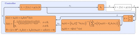
Figure 6: Closed-form optimal and safe control with input constraints. Control uses the composite soft-minimum CBF $\hat{h}$ to guarantee safety with input constraints. Control minimizes cost $\hat{J}$ subject to safety and input constraints.

Figure 6 illustrates the architecture of the control 37, 38, 28, 29, VI-C, 39, 49, 47, and 48. The following corollary is the main result on safety- and input-constraint satisfaction using this control. This corollary is a consequence of applying Theorem 2 to the cascade 31, 32, and 33.

Corollary 3.

Consider (2), where (A1) is satisfied, and consider $u$ given by 37, 38, 28, 29, VI-C, 39, 49, 47, and 48, where (C1) and (C2) are satisfied. Assume that $\hat{h}^{\prime}$ is locally Lipschitz on $\hat{\mathcal{S}}$, and for all $\hat{x}\in\hat{\mathcal{B}}$, $L_{\hat{g}}\hat{h}(\hat{x})\neq 0$. Let $\hat{x}_{0}\in\hat{\mathcal{S}}\cap\hat{\mathcal{C}}$. Then, for all $t\geq 0$, $\hat{x}(t)\in\hat{\mathcal{S}}\cap\hat{\mathcal{C}}$, $x(t)\in{\mathcal{S}}_{\rm s}$, and $u(t)\in{\mathcal{U}}$.

VI-E Ground Robot Example Revisited with Input Constraints

We present an example to demonstrate the control 37, 38, 28, 29, VI-C, 39, 49, 47, and 48.

Example 3.

We revisit the nonholonomic ground robot from Example 1 and include not only safety constraints but also input constraints. The safe set ${\mathcal{S}}_{\rm s}$ and the desired control $u_{\rm d}$ are the same as Example 1, that is, $h_{1},\ldots,h_{9}$ are given by 20, 21, and 22 and $u_{\rm d}$ is given by 23, 24, 25, and 26.

In this example, we also consider control input constraints. Specifically, the control must remain in the admissibile set ${\mathcal{U}}$ is given by (27), where

$$\phi_{1}(u) =4-u_{1},\qquad\phi_{2}(u)=u_{1}+4,$$

$$\phi_{3}(u) =1-u_{2},\qquad\phi_{4}(u)=u_{2}+1,$$

which implies ${\mathcal{U}}=\{u\in{\mathbb{R}}^{2}\colon|u_{1}|\leq 4\mbox{ and }|u_{2}|\leq 1\}$ and $\hat{\ell}=13$.

We consider the controller dynamics 28 and 29, where $f_{\rm c}$, $g_{\rm c}$, and $h_{\rm c}$ are given by Example 2 with $A_{\rm c}=-I_{2}$, $B_{\rm c}=I_{2}$, and $C_{\rm c}=I_{2}$. Thus, (C1) and (C2) are satisfied with $d_{\rm c}=1$ and $\zeta=1$, and it follows from Example 1 and (36) that $\hat{d}_{1}=\cdots\hat{d}_{7}=3$, $\hat{d}_{8}=\hat{d}_{9}=2$, and $\hat{d}_{10}=\cdots=\hat{d}_{13}=1$.

We implement the control 37, 38, 28, 29, VI-C, 39, 49, 47, and 48 with $\rho=10$, $\gamma=100$, $\hat{\alpha}_{1,0}(h)=\ldots=\hat{\alpha}_{6,0}(h)=h$, $\hat{\alpha}_{1,1}(h)=\ldots=\hat{\alpha}_{6,1}(h)=2.5h$, $\hat{\alpha}_{7,0}(h)=6h$, $\hat{\alpha}_{7,1}(h)=h$, $\hat{\alpha}_{8,0}(h)=\hat{\alpha}_{9,0}(h)=10h$, $\alpha=0$, and $\sigma_{0}=1$. The control is updated at $1~{}\rm{kHz}$.

Figure 7 shows the closed-loop trajectories for $\hat{x}_{0}=[\,-1\quad-8.5\quad 0\quad\frac{\pi}{2}\quad 0\quad 0\,]^{\rm T}$ with 4 different goal locations $q_{{\rm d}}=[\,3\quad 4.5\,]^{\rm T}$, $q_{{\rm d}}=[\,-7\quad 0\,]^{\rm T}$, $q_{{\rm d}}=[\,7\quad 1.5\,]^{\rm T}$, and $q_{{\rm d}}=[\,-1\quad 7\,]^{\rm T}$. In all cases, the robot position converges to the goal location while satisfying safety and input constraints.

Figures 8 and 9 show the trajectories of the relevant signals for the case where $q_{{\rm d}}=[\,3\quad 4.5\,]^{\rm T}$. Figure 9 shows that $\hat{h}$, $\min\hat{b}_{j,i}$, and $\min\hat{h}_{j}$ are positive for all time, which implies that $x$ remains in ${\mathcal{S}}_{\rm s}$ and $u$ remains in ${\mathcal{U}}$.  $\triangle$

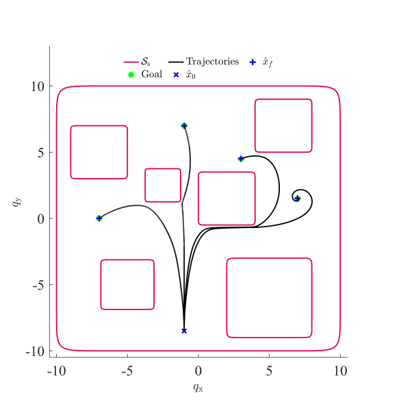
Figure 7: ${\mathcal{S}}_{\rm s}$ and closed-loop trajectories for 4 goal locations.

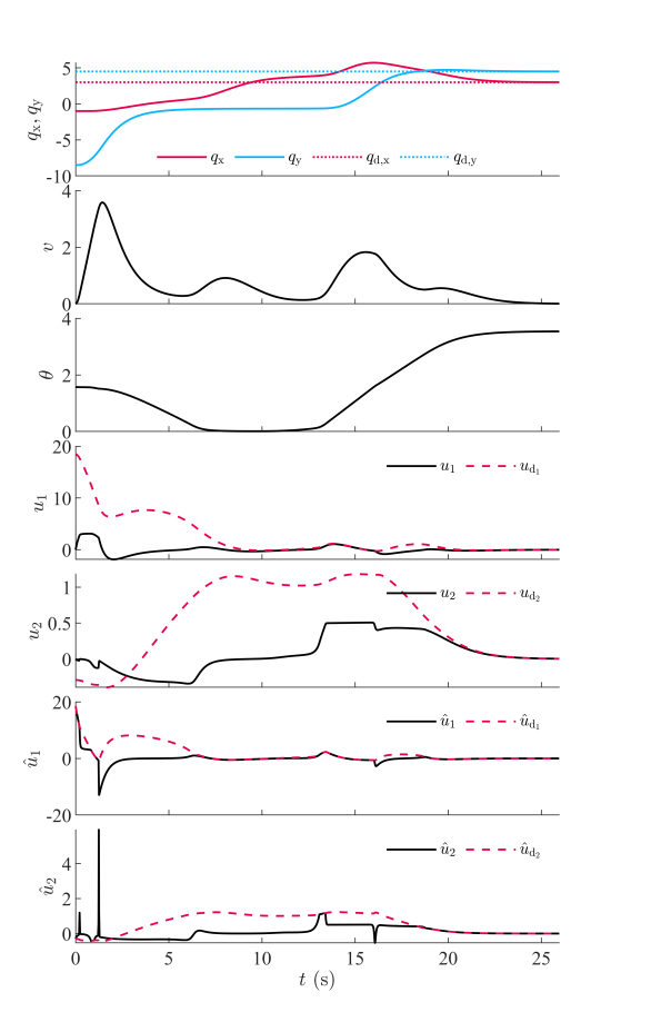
Figure 8: $q_{\rm x}$, $q_{\rm y}$, $v$, $\theta$, $u$, $u_{\rm d}$, $\hat{u}=[\,\hat{u}_{1}\quad\hat{u}_{2}\,]^{\rm T}$, and $\hat{u}_{\rm d}=[\,\hat{u}_{{\rm d}_{1}}\quad\hat{u}_{{\rm d}_{2}}\,]^{\rm T}$ for $q_{{\rm d}}=[\,3\quad 4.5\,]^{\rm T}$.

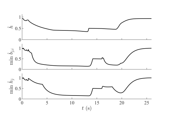
Figure 9: $\hat{h}$, $\min\hat{b}_{\hat{\jmath},i}$, and $\min\hat{h}_{\hat{\jmath}}$ for $q_{{\rm d}}=[\,3\quad 4.5\,]^{\rm T}$.

VII Concluding Remarks

This article presents several new contributions. First, Section IV presents a method for constructing a single composite soft-minimum CBF (10) from multiple CBFs, which can have different relative degrees. Proposition 2 is the main result of Section IV, and it shows that the zero-superlevel set of the composite soft-minimum CBF describes the control forward invariant set ${\mathcal{S}}\cap{\mathcal{C}}$, which is a subset of the safe set ${\mathcal{S}}_{\rm s}$. Next, Section V uses the composite soft-minimum CBF (10) in a constrained quadratic optimization to construct a closed-form optimal control that guarantees safety. Theorem 2 is the main result of Section V, and this theorem shows that the closed-form optimal control 6, 10, 16, 14, 15, 17, 18, and 19 guarantees safety. Finally, Section VI extends the approach to construct a closed-form optimal control that not only guarantees safety but also respects input constraints. The key elements in the development of this novel closed-form control include the introduction of the control dynamics 28 and 29 and the surrogate cost (45), and most importantly, the use of the composite soft-minimum CBF to compose safety and input constraints, which have different relative degrees, into a single CBF. Corollary 3 is the main result, which shows that the closed-form optimal control 37, 38, 28, 29, VI-C, 39, 49, 47, and 48 guarantees both safety- and input-constraint satisfaction.

We note that the approach in this paper to generate a closed-form control that satisfies safety and input constraints can be directly extended to address input rate constraints (and constraints on higher-order time derivatives of the input). To accomplish this, the control dynamics 28 and 29 are designed such that its relative degree $d_{\rm c}$ is greater than the positive integer $r$, where $\frac{{\rm d}^{r}}{{\rm d}t^{r}}u$ is the highest-order time derivative of the control that has a constraint. In this case, constraints on $u,\frac{{\rm d}}{{\rm d}t}u,\ldots,\frac{{\rm d}^{r}}{{\rm d}t^{r}}u$ are transformed into constraints on the controller state $x_{\rm c}$ using the approach in Section VI.

In this work, the log-sum-exponential soft minimum (1) is used to compose multiple state constraints and multiple input constraints into a single constraint. In other words, the zero-superlevel set of the soft minimum (1) is an approximation (subset) of the intersection of the zero-superlevel sets of the arguments of the soft minimum. See Proposition 1. Thus, the log-sum-exponential soft minimum can be used to approximate the intersection of zero-superlevel sets. Similarly, the log-sum-exponential soft maximum can be used to approximate the union of zero-superlevel sets. See [30] for more details.

Appendix A Relative Degree of a Nonlinear Cascade

This appendix examines the relative degree of a cascade of nonlinear systems. The results in this appendix are needed for Proposition 6 and Proposition 7 in Section VI. Consider

$$\dot{x}_{1}(t) =f_{1}(x_{1}(t))+g_{1}(x_{1}(t))u_{1}(t),$$ (50)

$$\dot{x}_{2}(t) =f_{2}(x_{2}(t))+g_{2}(x_{2}(t))u_{2}(t),$$ (51)

where for $i\in\{1,2\}$, $x_{i}(t)\in{\mathbb{R}}^{n_{i}}$ is the state, $x_{i}(0)=x_{i0}\in{\mathbb{R}}^{n_{i}}$ is the initial condition, and $u_{i}(t)\in{\mathbb{R}}^{m_{i}}$ is the input.

Let $\xi_{1}:{\mathbb{R}}^{n_{1}}\to{\mathbb{R}}^{l_{1}}$ and $\xi_{2}:{\mathbb{R}}^{n_{2}}\to{\mathbb{R}}^{m_{1}}$. We make the following assumption:

1. For $i\in\{1,2\}$, there exists ${\mathcal{X}}_{i}\in{\mathbb{R}}^{n_{i}}$ and a positive integer $r_{i}$ such that for all $x_{i}\in{\mathcal{X}}_{i}$, $L_{g_{i}}\xi_{i}(x_{i})=L_{g_{i}}L_{f_{i}}\xi_{i}(x_{i})=\cdots=L_{g_{i}}L_{f_{i}}^{r_{i}-2}\xi_{i}(x_{i})=0$ and $L_{g_{i}}L_{f_{i}}^{r_{i}-1}\xi_{i}(x_{i})\neq 0$.

Assumption (A2) implies that $\xi_{i}$ has relative degree $r_{i}$ with respect to $\dot{x}_{i}=f_{i}(x_{i})+g_{i}(x_{i})u_{i}$ on ${\mathcal{X}}_{i}$.

Next, we consider the cascade of (50) and (51), where $u_{1}=\xi_{2}(x_{2})$, which is given by

$$\dot{\hat{x}} =\hat{f}(\hat{x})+\hat{g}(\hat{x})u_{2},$$ (52)

$$y =\hat{h}(\hat{x}),$$ (53)

where

$$\hat{x}\triangleq\begin{bmatrix}x_{1}\\ x_{2}\end{bmatrix},\qquad\hat{f}(\hat{x})\triangleq\begin{bmatrix}f_{1}(x_{1})+g_{1}(x_{1})\xi_{2}(x_{2})\\ f_{2}(x_{2})\end{bmatrix},$$ (54)

$$\hat{g}(\hat{x})\triangleq\begin{bmatrix}0\\ g_{2}(x_{2})\end{bmatrix},\qquad\hat{h}(\hat{x})\triangleq\xi_{1}(x_{1}).$$ (55)

The following preliminary results are needed.

Lemma 2.

Consider 52, 53, 54, 55, 50, and 51, where (A2) is satisfied. For all $\hat{x}\in{\mathcal{X}}_{1}\times{\mathcal{X}}_{2}$, the following statements hold:

1. Let $j\in\{0,1,\ldots,r_{1}-1\}$. Then, $L_{\hat{f}}^{j}\hat{h}(\hat{x})=L_{f_{1}}^{j}\xi_{1}(x_{1})$.

2. Let $j\in\{0,1,\ldots,r_{1}-2\}$. Then, $L_{\hat{g}}L_{\hat{f}}^{j}\hat{h}(\hat{x})=0$.

Proof.

To prove (a), we use induction on $j$. First, note that $L_{\hat{f}}^{0}\hat{h}(\hat{x})=\hat{h}(\hat{x})=\xi_{1}(x_{1})=L_{f_{1}}^{0}\xi_{1}(x_{1})$, which implies that (a) holds for $j=0$. Next, assume that (a) holds for $j=a\in\{0,1,\ldots,r_{1}-2\}$. Thus,

$$L_{\hat{f}}^{a+1}\hat{h}(\hat{x})=L_{\hat{f}}L_{\hat{f}}^{a}\hat{h}(\hat{x})=L_{\hat{f}}L_{f_{1}}^{a}\xi_{1}(x_{1}),$$

which combined with (54) and (A2) yields

$$L_{\hat{f}}^{a+1}\hat{h}(\hat{x}) =L_{f_{1}}^{a+1}\xi_{1}(x_{1})+[L_{g_{1}}L_{f_{1}}^{a}\xi_{1}(x_{1})]\xi_{2}(x_{2})$$

$$=L_{f_{1}}^{a+1}\xi_{1}(x_{1}),$$

which confirms (a).

To prove (b), let $b\in\{0,1,\ldots,r_{1}-2\}$, and it follows from (a) that $L_{\hat{g}}L_{\hat{f}}^{b}\hat{h}(\hat{x})=L_{\hat{g}}L_{f_{1}}^{b}\xi_{1}(x_{1})=0$. ∎

Let $\nu:{\mathbb{R}}^{n_{1}}\to{\mathbb{R}}^{\ell_{1}}$ be continuously differentiable, and let $\hat{\nu}:{\mathbb{R}}^{n_{1}+n_{2}}\to{\mathbb{R}}^{\ell_{1}}$ be defined by $\hat{\nu}(\hat{x})\triangleq\nu(x_{1})$.

Lemma 3.

Let $j$ be a positive integer. Then, there exists $F_{j}:{\mathbb{R}}^{n_{1}\times m^{j-1}}\to{\mathbb{R}}^{\ell_{1}}$ such that for all $\hat{x}\in{\mathcal{X}}_{1}\times{\mathcal{X}}_{2}$,

$$L_{\hat{f}}^{j}\hat{\nu}(\hat{x}) =F_{j}\mathopen{}\mathclose{{}\left(x_{1},\xi_{2}(x_{2}),L_{f_{2}}\xi_{2}(x_{2}),\ldots,L_{f_{2}}^{j-2}\xi_{2}(x_{2})}\right)$$

$$\qquad+\mathopen{}\mathclose{{}\left[L_{g_{1}}\nu(x_{1})}\right]L_{f_{2}}^{j-1}\xi_{2}(x_{2}).$$ (56)

Proof.

We use induction on $j$. First, (54) implies that $L_{\hat{f}}\hat{\nu}(\hat{x})=L_{\hat{f}}\nu(x_{1})=L_{f_{1}}\nu(x_{1})+[L_{g_{1}}\nu(x_{1})]\xi_{2}(x_{2})=F_{1}(x_{1})+[L_{g_{1}}\nu(x_{1})]\xi_{2}(x_{2})$, where $F_{1}(x_{1})=L_{f_{1}}\nu(x_{1})$, which confirms (3) for $j=1$.

Next, assume that (3) holds for $j=a\in\{1,2,\ldots\}$. Thus,

$$L_{\hat{f}}^{a+1}\hat{\nu}(\hat{x}) =L_{\hat{f}}L_{\hat{f}}^{a}\hat{\nu}(\hat{x})$$

$$=L_{\hat{f}}F_{a}+L_{\hat{f}}\mathopen{}\mathclose{{}\left[L_{g_{1}}\nu(x_{1})L_{f_{2}}^{a-1}\xi_{2}(x_{2})}\right],$$ (57)

where the arguments of $F_{a}$ are omitted. Next, note that it follows from (54) that

$$L_{\hat{f}}F_{a} =\frac{\partial F_{a}}{\partial x_{1}}\mathopen{}\mathclose{{}\left[f_{1}(x_{1})+g_{1}(x_{1})\xi_{2}(x_{2})}\right]$$

$$\qquad+\sum_{k=0}^{a-2}\frac{\partial F_{a}}{\partial L_{f_{2}}^{k}\xi_{2}}\frac{\partial L_{f_{2}}^{k}\xi_{2}(x_{2})}{\partial x_{2}}f_{2}(x_{2})$$

$$=L_{f_{1}}F_{a}+\mathopen{}\mathclose{{}\left[L_{g_{1}}F_{a}}\right]\xi_{2}(x_{2})+\sum_{k=0}^{a-2}\frac{\partial F_{j}}{\partial L_{f_{2}}^{k}\xi_{2}}L_{f_{2}}^{k+1}\xi(x_{2}).$$ (58)

and

$$L_{\hat{f}}\mathopen{}\mathclose{{}\left[L_{g_{1}}\nu(x_{1})L_{f_{2}}^{a-1}\xi_{2}(x_{2})}\right] =\mathopen{}\mathclose{{}\left(I_{\ell_{1}}\otimes L_{f_{2}}^{a-1}\xi_{2}(x_{2})}\right)^{\rm T}G(x_{1})$$

$$\qquad\times\mathopen{}\mathclose{{}\left(f_{1}(x_{1})+g_{1}(x_{1})\xi_{2}(x_{2})}\right)$$

$$\qquad+L_{g_{1}}\nu(x_{1})L_{f_{2}}^{a}\xi_{2}(x_{2}),$$ (59)

where $\otimes$ is the Kronecker product,

$$G(x_{1})\triangleq\begin{bmatrix}\frac{\partial}{\partial x_{1}}\mathopen{}\mathclose{{}\left[L_{g_{1}}\nu(x_{1})}\right]_{(1)}^{\rm T}\\ \vdots\\ \frac{\partial}{\partial x_{1}}\mathopen{}\mathclose{{}\left[L_{g_{1}}\nu(x_{1})}\right]_{(\ell_{1})}^{\rm T}\\ \end{bmatrix},$$

and $\mathopen{}\mathclose{{}\left[L_{g_{1}}\nu(x_{1})}\right]_{(i)}$ is the $i$th row of $L_{g_{1}}\nu(x_{1})$. Thus, substituting 58 and A into (57) yields

$$L_{\hat{f}}^{a+1}\hat{\nu}(\hat{x})=F_{a+1}+L_{g_{1}}\nu(x_{1})L_{f_{2}}^{a}\xi_{2}(x_{2}),$$

where

$$F_{a+1} =L_{f_{1}}F_{a}+\mathopen{}\mathclose{{}\left[L_{g_{1}}F_{a}}\right]\xi_{2}(x_{2})+\sum_{k=0}^{a-2}\frac{\partial F_{j}}{\partial L_{f_{2}}^{k}\xi_{2}}L_{f_{2}}^{k+1}\xi(x_{2})$$

$$\qquad+\mathopen{}\mathclose{{}\left(I_{\ell_{1}}\otimes L_{f_{2}}^{a-1}\xi_{2}(x_{2})}\right)^{\rm T}G(x_{1})$$

$$\qquad\times\mathopen{}\mathclose{{}\left(f_{1}(x_{1})+g_{1}(x_{1})\xi_{2}(x_{2})}\right),$$

which confirms (3) for $j=a+1$. ∎

Lemma 4.

Consider 50, 51, 52, 53, 54, and 55, where (A2) is satisfied. For all $\hat{x}\in{\mathcal{X}}_{1}\times{\mathcal{X}}_{2}$, the following statements hold:

1. For $j\in\{0,1,\ldots,r_{2}-1\}$, $L_{\hat{g}}L_{\hat{f}}^{j}\hat{\nu}(\hat{x})=0$.

2. $L_{\hat{g}}L_{\hat{f}}^{r_{2}}\hat{\nu}(\hat{x})=\mathopen{}\mathclose{{}\left[L_{g_{1}}\nu(x_{1})}\right]L_{g_{2}}L_{f_{2}}^{r_{2}-1}\xi_{2}(x_{2})$.

Proof.

It follows from Lemma 3 that for all positive integers $a$,

$$L_{\hat{g}}L_{\hat{f}}^{a}\hat{\nu}(\hat{x}) =L_{\hat{g}}F_{a}(x_{1},L_{f_{2}}^{0}\xi_{2}(x_{2}),\ldots,L_{f_{2}}^{a-2}\xi_{2}(x_{2}))$$

$$\qquad+L_{\hat{g}}\mathopen{}\mathclose{{}\left(\mathopen{}\mathclose{{}\left[L_{g_{1}}\nu(x_{1})}\right]L_{f_{2}}^{a-1}\xi_{2}(x_{2})}\right).$$ (60)

To prove (a), let $j\in\{0,1,\ldots,r_{2}-1\}$. Note that (55) and (A2) imply that $L_{\hat{g}}F_{j}(x_{1},\xi_{2}(x_{2}),\ldots,L_{f_{2}}^{j-2}\xi_{2}(x_{2}))=0$ and $L_{\hat{g}}([L_{g_{1}}\nu(x_{1})]L_{f_{2}}^{j-1}\xi_{2}(x_{2}))=0$, which together with (A) confirms (a).

To prove (b), it follows from (55) and (A2) that $L_{\hat{g}}F_{r_{2}}(x_{1},\xi_{2}(x_{2}),\ldots,L_{f_{2}}^{r_{2}-2}\xi_{2}(x_{2}))=0$ and $L_{\hat{g}}([L_{g_{1}}\nu(x_{1})]L_{f_{2}}^{r_{2}-1}\xi_{2}(x_{2}))=[L_{g_{1}}\nu(x_{1})]L_{g_{2}}L_{f_{2}}^{r_{2}-1}\xi_{2}(x_{2})$, which together with (A) confirms (a). ∎

The following result shows that the relative degree of the cascade is greater than or equal to the sum of the relative degrees. Furthermore, the relative degree of the cascade is equal to sum of the relative degrees if and only if $[L_{g_{1}}L_{f_{1}}^{r_{1}-1}h_{1}(x_{1})]L_{g_{2}}L_{f_{2}}^{r_{2}-1}h_{2}(x_{2})$ is nonzero.

Theorem 3.

Consider 52, 53, 54, 55, 50, and 51, where (A2) is satisfied. Then, for all $\hat{x}\in{\mathcal{X}}_{1}\times{\mathcal{X}}_{2}$, the following statements hold:

1. For all $j\in\{0,1,\ldots,r_{1}+r_{2}-2\}$, $L_{\hat{g}}L_{\hat{f}}^{j}\hat{h}(\hat{x})=0$.

2. $L_{\hat{g}}L_{\hat{f}}^{r_{1}+r_{2}-1}\hat{h}(\hat{x})=[L_{g_{1}}L_{f_{1}}^{r_{1}-1}\xi_{1}(x_{1})]L_{g_{2}}L_{f_{2}}^{r_{2}-1}\xi_{2}(x_{2})$.

Proof.

Define $\nu(x_{1})\triangleq L_{f_{1}}^{r_{1}-1}\xi_{1}(x_{1})$ and $\hat{\nu}(\hat{x})\triangleq\nu(x_{1})$.

To prove (a), it follows from Lemma 2 that for all $j\in\{0,\ldots,r_{1}-2\}$, $L_{\hat{g}}L_{\hat{f}}^{j}\hat{h}(\hat{x})=0$.

Next, let $a\in\{r_{1}-1,r_{1},\ldots,r_{1}+r_{2}-2\}$ and define $b\triangleq a-r_{1}+1$. Thus, $L_{\hat{g}}L_{\hat{f}}^{a}\hat{h}(\hat{x})=L_{\hat{g}}L_{\hat{f}}^{b}L_{\hat{f}}^{r_{1}-1}\hat{h}(\hat{x})=L_{\hat{g}}L_{\hat{f}}^{b}\hat{\nu}(\hat{x})$. Since, in addition, $b\in\{0,\ldots,r_{2}-1\}$, it follows from Lemma 4 that $L_{\hat{g}}L_{\hat{f}}^{a}\hat{h}(\hat{x})=0$, which implies that for all $j\in\{r_{1}-1,r_{1},\ldots,r_{1}+r_{2}-2\}$, $L_{\hat{g}}L_{\hat{f}}^{j}\hat{h}(\hat{x})=0$.

To prove (b), note that $L_{\hat{g}}L_{\hat{f}}^{r_{1}+r_{2}-1}\hat{h}(\hat{x})=L_{\hat{g}}L_{\hat{f}}^{r_{2}}L_{\hat{f}}^{r_{1}-1}\hat{h}(\hat{x})=L_{\hat{g}}L_{\hat{f}}^{r_{2}}\hat{\nu}(\hat{x})$. Thus, Lemma 4 implies that $L_{\hat{g}}L_{\hat{f}}^{r_{1}+r_{2}-1}\hat{h}(\hat{x})=[L_{g_{1}}\nu(x_{1})]L_{g_{2}}L_{f_{2}}^{r_{2}-1}\xi_{2}(x_{2})=[L_{g_{1}}L_{f_{1}}^{r_{1}-1}\xi_{1}(x_{1})]L_{g_{2}}L_{f_{2}}^{r_{2}-1}\xi_{2}(x_{2})$. ∎

References

- [1] A. D. Ames, X. Xu, J. W. Grizzle, P. Tabuada, Control barrier function based quadratic programs for safety critical systems, IEEE Trans. Autom. Contr. (2016) 3861–3876.
- [2] X. Xu, P. Tabuada, J. W. Grizzle, A. D. Ames, Robustness of control barrier functions for safety critical control, IFAC-PapersOnLine 48 (27) (2015) 54–61.
- [3] K. P. Wabersich, M. N. Zeilinger, Predictive control barrier functions: Enhanced safety mechanisms for learning-based control, IEEE Trans. Autom. Contr. (2022).
- [4] X. Xu, J. W. Grizzle, P. Tabuada, A. D. Ames, Correctness guarantees for the composition of lane keeping and adaptive cruise control, IEEE Trans. Auto. Sci. and Eng. (2017) 1216–1229.
- [5] P. Seiler, M. Jankovic, E. Hellstrom, Control barrier functions with unmodeled input dynamics using integral quadratic constraints, IEEE Contr. Sys. Let. 6 (2021) 1664–1669.
- [6] J. Breeden, D. Panagou, Robust control barrier functions under high relative degree and input constraints for satellite trajectories, Automatica 155 (2023) 111109.
- [7] Q. Nguyen, K. Sreenath, Exponential control barrier functions for enforcing high relative-degree safety-critical constraints, in: Proc. Amer. Contr. Conf. (ACC), IEEE, 2016, pp. 322–328.
- [8] M. Z. Romdlony, B. Jayawardhana, Stabilization with guaranteed safety using control lyapunov–barrier function, Automatica 66 (2016) 39–47.
- [9] S. Prajna, A. Jadbabaie, G. J. Pappas, A framework for worst-case and stochastic safety verification using barrier certificates, IEEE Trans. Autom. Contr. (2007) 1415–1428.
- [10] D. Panagou, D. M. Stipanović, P. G. Voulgaris, Distributed coordination control for multi-robot networks using Lyapunov-like barrier functions, IEEE Trans. Autom. Contr. (2015) 617–632.
- [11] K. P. Tee, S. S. Ge, E. H. Tay, Barrier Lyapunov functions for the control of output-constrained nonlinear systems, Automatica (2009) 918–927.
- [12] X. Jin, Adaptive fixed-time control for MIMO nonlinear systems with asymmetric output constraints using universal barrier functions, IEEE Trans. Autom. Contr. (2018) 3046–3053.
- [13] Q. Nguyen, K. Sreenath, Safety-critical control for dynamical bipedal walking with precise footstep placement, IFAC-PapersOnLine (2015) 147–154.
- [14] M. Srinivasan, S. Coogan, Control of mobile robots using barrier functions under temporal logic specifications, IEEE Trans. on Rob. 37 (2) (2020) 363–374.
- [15] Z. Jian, Z. Yan, X. Lei, Z. Lu, B. Lan, X. Wang, B. Liang, Dynamic control barrier function-based model predictive control to safety-critical obstacle-avoidance of mobile robot, in: Proc. Int. Rob. Autom. (ICRA), IEEE, 2023, pp. 3679–3685.
- [16] A. Safari, J. B. Hoagg, Time-varying soft-maximum control barrier functions for safety in an a priori unknown environment, arXiv preprint arXiv:2310.05261 (2023).
- [17] U. Borrmann, L. Wang, A. D. Ames, M. Egerstedt, Control barrier certificates for safe swarm behavior, IFAC-PapersOnLine (2015) 68–73.
- [18] A. Singletary, A. Swann, Y. Chen, A. D. Ames, Onboard safety guarantees for racing drones: High-speed geofencing with control barrier functions, IEEE Rob. and Autom. Let. 7 (2) (2022) 2897–2904.
- [19] J. Seo, J. Lee, E. Baek, R. Horowitz, J. Choi, Safety-critical control with nonaffine control inputs via a relaxed control barrier function for an autonomous vehicle, IEEE Rob. and Auto. Let. 7 (2) (2022) 1944–1951.
- [20] A. Alan, A. J. Taylor, C. R. He, A. D. Ames, G. Orosz, Control barrier functions and input-to-state safety with application to automated vehicles, IEEE Trans. on Contr. Sys. Tech. (2023).
- [21] R. Wisniewski, C. Sloth, Converse barrier certificate theorems, IEEE Trans. Autom. Contr. (2015) 1356–1361.
- [22] L. Wang, D. Han, M. Egerstedt, Permissive barrier certificates for safe stabilization using sum-of-squares, in: 2018 Amer. Contr. Conf. (ACC), 2018, pp. 585–590.
- [23] A. Clark, Verification and synthesis of control barrier functions, in: Proc. Conf. Dec. Contr. (CDC), 2021, pp. 6105–6112.
- [24] A. Isaly, M. Ghanbarpour, R. G. Sanfelice, W. E. Dixon, On the feasibility and continuity of feedback controllers defined by multiple control barrier functions for constrained differential inclusions, in: 2022 Amer. Contr. Conf. (ACC), IEEE, 2022, pp. 5160–5165.
- [25] E. Pond, M. Hale, Fast verification of control barrier functions via linear programming, arXiv preprint arXiv:2212.00598 (2022).
- [26] X. Tan, D. V. Dimarogonas, Compatibility checking of multiple control barrier functions for input constrained systems, in: Proc. Conf. Dec. Contr. (CDC), IEEE, 2022, pp. 939–944.
- [27] T. Gurriet, M. Mote, A. Singletary, P. Nilsson, E. Feron, A. D. Ames, A scalable safety critical control framework for nonlinear systems, IEEE Access (2020) 187249–187275.
- [28] Y. Chen, A. Singletary, A. D. Ames, Guaranteed obstacle avoidance for multi-robot operations with limited actuation: A control barrier function approach, IEEE Contr. Sys. Let. (2020) 127–132.
- [29] P. Rabiee, J. B. Hoagg, Soft-minimum barrier functions for safety-critical control subject to actuation constraints, in: Proc. Amer. Contr. Conf. (ACC), 2023, pp. 2646–2651.
- [30] P. Rabiee, J. B. Hoagg, Soft-minimum and soft-maximum barrier functions for safety with actuation constraints, arXiv preprint arXiv:2305.10620 (2023).
- [31] M. Black, D. Panagou, Consolidated control barrier functions: Synthesis and online verification via adaptation under input constraints, arXiv preprint arXiv:2304.01815 (2023).
- [32] W. Xiao, C. G. Cassandras, C. A. Belta, D. Rus, Control barrier functions for systems with multiple control inputs, in: 2022 Amer. Contr. Conf. (ACC), IEEE, 2022, pp. 2221–2226.
- [33] A. D. Ames, G. Notomista, Y. Wardi, M. Egerstedt, Integral control barrier functions for dynamically defined control laws, IEEE Contr. Sys. Let. 5 (3) (2020) 887–892.
- [34] P. Rabiee, J. B. Hoagg, Composition of control barrier functions with differing relative degrees for safety under input constraints, arXiv preprint arXiv:2310.00363 (2023).
- [35] X. Tan, W. S. Cortez, D. V. Dimarogonas, High-order barrier functions: Robustness, safety, and performance-critical control, IEEE Trans. Autom. Contr. 67 (6) (2021) 3021–3028.
- [36] F. Blanchini, S. Miani, et al., Set-theoretic methods in control, Vol. 78, Springer, 2008.
- [37] A. De Luca, G. Oriolo, M. Vendittelli, Control of wheeled mobile robots: An experimental overview, RAMSETE (2002) 181–226.