StableNormal: Reducing Diffusion Variance for Stable and Sharp Normal

Abstract.

This work addresses the challenge of high-quality surface normal estimation from monocular colored inputs (i.e., images and videos), a field which has recently been revolutionized by repurposing diffusion priors. However, previous attempts still struggle with stochastic inference, conflicting with the deterministic nature of the Image2Normal task, and costly ensembling step, which slows down the estimation process. Our method, StableNormal, mitigates the stochasticity of the diffusion process by reducing inference variance, thus producing “Stable-and-Sharp” normal estimates without any additional ensembling process. StableNormal works robustly under challenging imaging conditions, such as extreme lighting, blurring, and low quality. It is also robust against transparent and reflective surfaces, as well as cluttered scenes with numerous objects. Specifically, StableNormal employs a coarse-to-fine strategy, which starts with a one-step normal estimator (YOSO) to derive an initial normal guess, that is relatively coarse but reliable, then followed by a semantic-guided refinement process (SG-DRN) that refines the normals to recover geometric details. The effectiveness of StableNormal is demonstrated through competitive performance in standard datasets such as DIODE-indoor, iBims, ScannetV2 and NYUv2, and also in various downstream tasks, such as surface reconstruction and normal enhancement. These results evidence that StableNormal retains both the “stability” and “sharpness” for accurate normal estimation. StableNormal represents a baby attempt to repurpose diffusion priors for deterministic estimation. To democratize this, code and models have been publicly available in hf.co/Stable-X.

Figure 1. We propose StableNormal, which tailors the diffusion priors for monocular normal estimation. Unlike prior diffusion-based works, we focus on enhancing estimation stability by reducing the inherent stochasticity of diffusion models (i.e., Stable Diffusion (Rombach et al., 2021)). This enables “Stable-and-Sharp” normal estimation, which outperforms multiple baselines (try Compare), and improves various real-world applications (try Demo).

1. Introduction

Normal map, as a 2.5D representation, bridges 2D and 3D worlds. In 3D modeling, object surfaces are typically represented by polygons. Normal maps add illusory surface details to these polygons, which enhances their realism. In 2D domain, if accurately estimated from in-the-wild pixels, tasks such as relighting or intrinsic decomposition become feasible, opening the door to a broad spectrum of applications. StableNormal aims to estimate accurate & sharp surface normals from monocular colored inputs (i.e., images, videos).

In the era of deep learning, this “Image2Normal” task has been well explored in a line of works (Fouhey et al., 2013a; Eftekhar et al., 2021; Eigen and Fergus, 2015a; Bansal et al., 2016a; Ranftl et al., 2021a; Wang et al., 2015a). Recently, advances in diffusion-based image generator, often trained on large-scale datasets (Schuhmann et al., 2022), have shifted the vision community’s focus towards repurposing the diffusion priors (Rombach et al., 2022a) to estimate the geometric or intrinsic cues, such as depth (Ke et al., 2024a), normal (Fu et al., 2024b), and materials (Kocsis et al., 2024).

These efforts have yielded “sharp-looking” results (Fig. 3). However, human eyes lack the sensitivity to accurately perceive the normal maps. Despite producing “sharp-looking” normals, temporal inconsistency exists , and the results, even after being ensembled, still deviate significantly from ground-truth normals (Fig. 3). Simply put, these results are “sharp” but neither “correct” nor “stable”.

We attribute this to two factors: 1) unstable imaging conditions, such as extreme lighting, dramatic camera movement, motion blur, and low-quality images. 2) inductive bias of the diffusion process — stochasticity. Such stochasticity contradicts the nature of the estimation process, which should be as deterministic as possible. Therefore, a crucial question is raised:

How can we mitigate the inherent stochasticity of the diffusion process for deterministic estimation?

Answering this question in the normal domain is more urgent than in depth domain. Since monocular depth estimation typically estimates affine-invariant depth (i.e., depth values up to a global offset and scale), while surface normals are not subject to scale and translation ambiguity. That is to say, given a single image, the task of normal estimation (one-to-one mapping), is more “deterministic” than depth estimation (one-to-many mapping). However, eliminating stochasticity from the diffusion process, like the one-step GenPercept (Xu et al., 2024), could compromise the recovery of high-frequency details and result in overly-smooth normals (See Fig. 2). Thus, finding a balance between “stability” vs. “sharpness” is needed.

Input	GenPercept	GeoWizard	Ours
	(Xu et al., 2024)	(Fu et al., 2024b)

Figure 2. Comparative Analysis of Normal Estimators: “Stability” vs. “Sharpness”. One-step GenPercept compromises the high-frequency details and produces overly-smooth normals for objects on the table, while GeoWizard produces seemingly sharp normals, but neither correct nor stable. Our method well balances stability and sharpness. The red boxes highlight the visual difference mentioned above.

Figure 3. High-variance normal estimations. We show multiple samples for a single scene and visualize the mean and variance of the predicted normals. For each sample, while the normal maps exhibit sharp details, there is high variance in areas with high-frequency content. This high variance in sharp regions makes the inference less reliable.

So we present StableNormal to tackle this trade-off. It demonstrates that, a reliable initialization, coupled with a stable refinement, is essential to produce sharp and stable normal estimates. Our approach follows the coarse-to-fine scheme: 1) one-step normal estimation (Section 3.3) for reliable initialization, and 2) semantic-guided diffusion refinement (Section 3.4) to progressively sharpen the normal maps in a semantic-aware direction.

Specifically, a Shrinkage Regularizer is introduced to train the one-step normal estimator, which reduces the training variance by splitting the vanilla diffusion loss into generative and reconstruction terms. This one-step estimator, namely YOSO (You-Only-Sample-Once), already performs on-par with current state-of-the-art DSINE (Bae and Davison, 2024), see Table 3. Additionally, Semantic-Guided Diffusion Refinement Network (SG-DRN) is presented to enhance the stability of the diffusion-based refinement process by integrating DINO semantic priors. Such priors decrease sampling variance while enhancing local details, as shown in Fig. 6.

We evaluate StableNormal on DIODE-indoor, iBims, ScannetV2, and NYUv2 datasets. Also, we show how our strong normal estimator improves various reconstruction scenarios (i.e., object-level, indoor-scene, and normal integration-based). The superiority of StableNormal is substantiated both qualitatively and quantitatively. Please check the video and Fig. 1 to see how robust StableNormal performs in challenging conditions, such as extreme lighting, blurring, object transparency & reflections, or clustered scenes.

The main contributions of StableNormal are as follows:

• We pinpoint the critical issue why diffusion priors cannot be directly (w/o bells and whistles, e.g. post-ensembling) applied on “Image2Normal” task — the inherent conflict between the “stochastic” diffusion process and “deterministic” requirement for geometric cues estimation.

• To address this conflict, we propose a simple-yet-effective solution, namely “StableNormal”. It justifies that a reliable initialization (YOSO), coupled with a stable refinement (SG-DRN), is essential to estimate sharp normals steadily.

• We conduct extensive experiments to evaluate StableNormal’s accuracy. It not only outperforms other baselines by a large margin in high-quality indoor benchmarks (i.e., DIODE-indoor, iBims, and ScannetV2), but also far ahead of its peers (i.e., GeoWizard, DSINE) in terms of inference stability at real-world scenarios, even under extreme conditions. This stability benefits many downstream tasks, see Fig. 1.

2. Related Works

2.1. Regression-based Monocular Normal Estimation

Surface normal estimation from monocular RGB inputs has been extensively studied  (Fouhey et al., 2013b, 2014; Ladický et al., 2014; Wang et al., 2015b; Eigen and Fergus, 2015b; Wang et al., 2016; Qi et al., 2018; Huang et al., 2019; Zhang et al., 2019; Liao et al., 2019; Qi et al., 2022; Do et al., 2020; Wang et al., 2020). In general, the prior regression-based methods consist of a feature extractor, followed by a prediction head. Hoiem et al. (Hoiem et al., 2005, 2007) were the pioneers in framing this classic task as a statistical learning problem. The output space was discretized, and handcrafted features were extracted to classify the normals. However, such features are generally designed for specific scenarios and cannot generalize well to unseen scenes.

This generalization problem was later addressed by deep learning techniques in a data-driven manner (Bansal et al., 2016b; Wang et al., 2015b). More recently, Omnidata-V2 (Eftekhar et al., 2021), with a U-Net architecture (Ronneberger et al., 2015), is trained on a large-scale data (12M) captured from diverse scenes under various camera settings. Bae et al. (Bae et al., 2021) propose to estimate the per-pixel surface normal probability distribution, from which the expected angular error can be inferred to quantify the aleatoric uncertainty. The transition from CNNs to vision transformers (ViT) has further advanced this field, as demonstrated by DPT (Ranftl et al., 2021b). DSINE (Bae and Davison, 2024) rethinks how to correctly model the inductive biases for surface normal estimation, and proposes to leverage the per-pixel ray direction, and learn the relative rotation between nearby pixels. These efforts decrease the need for large-scale training data, DSINE trained only on 160K images surpass the Omnidata-V2, which is trained on over 12M images. Recently, inspired by visual prompting (Bar et al., 2022), background prompting (Baradad et al., 2023) was introduced to reduce the domain gap between synthetic and real data, by simply placing the segmented object into a learned background “prompt”. Despite steady advancements, regression-based normal estimators, trained on limited and constrained data, continue to face generalization issues and struggle to capture fine-grained geometric details.

2.2. Diffusion-based Monocular Normal Estimation

Recently, the computer vision community has witnessed the bloom of diffusion-based Text-to-Image (T2I) model and its extensions (Rombach et al., 2021; Zhang et al., 2023a; Peebles and Xie, 2022). Several works have explored how to adapt the strong pretrained model, thus repurpose it as geometric cues estimator (Ji et al., 2023; Ke et al., 2024b; Zhao et al., 2023; Liu et al., 2023; Long et al., 2023; Qiu et al., 2024; Fu et al., 2024b). Wonder3D (Long et al., 2023) proposes to model the joint distribution of color and normal to enhance their consistency, which has been shown to improve the quality of the final 3D output. Richdreamer (Qiu et al., 2024) concurrently trains a depth and normal diffusion model on the large-scale LAION-2B dataset (Schuhmann et al., 2022), utilizing predictions from the off-the-shelf normal and depth estimators (Lasinger et al., 2019). Moreover, Geowizard (Fu et al., 2024b) extends Wonder3D by adding a geometry switcher (indoor/outdoor/object) to segregate the multi-sourced data distribution of various scenes into distinct sub-distributions.

Although these diffusion-based approaches can capture “sharp-looking” surface details, these results actually deviates significantly from ground-truth in normal space, owing to to the inherent high-variance of diffusion process (see Fig. 3). The large variance is first introduced by Gaussian initialization, which is propagated and amplified in the entire multi-step diffusion process (i.e., signal-leak issue (Everaert et al., 2024)). In fact, some prior research has explored this issue, either employing an affine-invariant ensembling strategy during the post-processing stage (Ke et al., 2024a; Fu et al., 2024b), or completely discarding the iterative multi-step generation process, thus shifting towards a one-step perception problem (Xu et al., 2024).

However, both strategies come with their own pitfalls: post-ensembling, which applies to multiple outputs, is computationally intensive. The assumption of affine invariance often fails to generalize across different types of outputs, like normals. While GeoWizard (Fu et al., 2024b) exhibits sharper results compared to other traditional approaches, it does not notably improve quantitative performance, suggesting that diffusion-based normal estimators induce the directional deviation in normal space (see Fig. 3). Furthermore, without the post-ensembling step, the diffusion-based estimators tend to produce outputs with large variance (see Fig. 3), highlighting its inherent stochastic nature. Regarding the one-step approach, it oversimplifies the markov chain of the diffusion process, smoothing out intrinsic local geometric details, leading to the typical over-smoothing artifacts seen in other regression-based methods (Bae and Davison, 2024; Eftekhar et al., 2021). Therefore, when repurposing the diffusion model for deterministic estimation tasks, such as normal estimation, a trade-off between “stability” and “sharpness” arises, which requires careful consideration before proceeding.

3. Method

Figure 4. Overview of the StableNormal. The overall pipeline is composed of two stages: 1) YOSO aims to produce a confident initialization $x_{t^{+}}$ for stage two with a novel Shrinkage Regularizer; 2) SG-DRN plays the role of stable denoising, by leveraging the stronger semantic control information extracted from DINO (Oquab et al., 2024). The textual prompt for the U-Net in both stages is set to “The normal map”.

3.1. Preliminaries on Diffusion Model

Diffusion Probabilistic Models (Ho et al., 2020; Song et al., 2020) aim to model a data distribution $p(x)$ by sequentially transform a Gaussian distribution via the so-called backward diffusion process $x_{t-1}=B_{t}x_{t}-\mu_{\theta}^{\epsilon}(x_{t},t)+\epsilon_{t}$ in which $\epsilon_{t}\sim\mathcal{N}(0,\sigma_{t}I)$ and $\mu_{\theta}^{\epsilon}$ predicts the injected noise. This backward process is uniquely determined by a predefined forward diffusion process $x_{t+1}=A_{t}x_{t}+\epsilon_{t}$.

As a classical example, DDPM (Ho et al., 2020) assumes that the initial Gaussian distribution $\mathcal{N}(\mathbf{0},\mathbf{I})$ can be obtained by running the following forward diffusion process:

(1) $$q(x_{t})=\sqrt{\alpha_{t}}{x_{0}}+\sqrt{1-\alpha_{t}}\bm{\epsilon},x_{0}\sim p(x),t\in\{0,1,...,T\}$$

where $\bm{\epsilon}\sim\mathcal{N}(\mathbf{0},\mathbf{I})$, $T$ denotes the number of the time step, t is the current time step, and $\alpha_{t}$ is the noise schedule controlling how fast the data distribution is transformed into a standard Gaussian distribution. As a result, the backward diffusion process in DDPM proves to be

(2) $$x_{t-1}=\frac{1}{\sqrt{\alpha_{t}}}x_{t}-\frac{1-\alpha_{t}}{\sqrt{\alpha_{t}(1-\Pi_{\tau=0}^{t}\alpha_{\tau})}}\mu_{\theta}^{\epsilon}(x_{t},t;)+\sigma_{t}\epsilon$$

The loss function for DDPM is a denosing autoencoder loss:

(3) $$L_{\theta}=\mathbb{E}_{\bm{x}_{0},\bm{c},t}\left\|\bm{x}_{0}-{\bm{\mu}_{\theta}}^{\bm{x}_{0}}(\bm{x}_{t},\bm{c},t)\right\|^{2}$$

Reparameterization. It is often convenient to reparameterize diffusion models as predicting the one-step denoised output (called $x_{0}$-reparameterization) instead of the injected noise (the default $\bm{\epsilon}$-reparameterization). In DDPM, $x_{t}=\sqrt{\alpha_{t}}x_{0}+\epsilon_{t}$ and therefore loss for $\bm{\epsilon}$-reparameterization is (up to a scale)

(4) $$L_{\theta}=\mathbb{E}_{\bm{\epsilon},\bm{c},t}\left\|\bm{\epsilon}-{\bm{\mu}_{\theta}}^{\bm{\epsilon}}(\bm{x}_{t},\bm{c},t)\right\|^{2}$$

Diffusion Samplers. When the number of time steps $T$ is large enough, both the forward diffusion process and the backward one can be seen as approximations of their continuous counterparts that can be modeled by stochastic differential equations (SDEs). It is therefore possible to sample from a trained DDPM model with SDE solvers or samplers other than the default DDPM backward diffusion process for better efficiency (at a cost of precision). As an example, DDIM generates samples with

(5) $$x_{t-1}=\sqrt{\alpha_{t-1}}\cdot\left(\frac{x_{t}-\sqrt{1-\alpha_{t}}\cdot{\bm{\mu}_{\theta}}^{\bm{\epsilon}}(x_{t},\bm{c},t)}{\sqrt{\alpha_{t}}}\right)+\textit{direction}(x_{t})+\tau\bm{\epsilon}$$

where $\tau$ is a scalar to control the amount of injected noise during the process. Notably, if $\tau$ is set to 0, DDIM becomes a deterministic sampler (i.e., independent of any noise).

Text-to-image (T2I) diffusion models.. Different from unconditional diffusion models, T2I diffusion models aim to generate images with optional text prompts. A classical example is Stable Diffusion (SD) (Rombach et al., 2021), a diffusion model $\mu_{\theta}(z_{t},t,c)$ built with a U-Net architecture and trained on the latent space of a pretrained VAE, in which $c$ is the additional text prompt embedding (typically obtained by CLIP (Radford et al., 2021)).

3.2. Diffusion-based Normal Estimator

Apart from common multi-modal generation tasks (e.g., text-to-image (Rombach et al., 2021), text-to-3D (Poole et al., 2023)), the pre-trained diffusion models have also proven to have surprisingly good zero-shot performance in several discriminative tasks, such as classification (Li et al., 2023b), and segmentation (Li et al., 2023c; Tian et al., 2024). And since image-to-image translation could be considered as a single-modal generation task, different 2D modalities (e.g., image, normal, depth, canny edge) could also be interconverted (Zhang et al., 2023a; Ke et al., 2024a; Wang et al., 2023) with the adapted or fine-tuned SD model.

Normal Estimation with SD. Since normal estimation can be seen as translating an RGB image into a normal map image, the diffusion prior from SD can also be effectively utilized. A straightforward approach is to take the RGB image as the conditioning signal to generate the corresponding normal maps, as in GeoWizard (Fu et al., 2024b) and Marigold (Ke et al., 2024a). More specifically, the condition signal is computed by first encoding the RGB input image $\bm{I}$ into a latent code with a pre-trained VAE encoder, namely $En$, and then, similar to ControlNet (Zhang et al., 2023a), we transform this latent code $En(\bm{I})$ through an additional encoder $f_{\phi}$, into the control signal for the decoder blocks of the U-Net in SD. The decoder blocks of U-Net, which is parameterized by $\theta$, and encoder $f_{\phi}$ are trained with the following loss (in $\bm{\epsilon}$-reparameterization):

(6) $$L_{\theta,\phi}=\mathbb{E}_{\bm{\epsilon},\bm{c},\bm{I},t}\left\|\bm{\epsilon}-{\bm{\mu}_{\theta}}^{\bm{\epsilon}}(\bm{x}_{t},\bm{c},t,f_{\phi}(En(\bm{I})))\right\|^{2}$$

where $\bm{I}$ is the input image, $x_{t}=q(En(N_{\text{gt}}))$ is the latent feature encoded from the ground truth normal map $N_{\text{gt}}$ at time step $t$.

During inference, it is straightforward to estimate the normal map for a given RGB image by running anyway sampling algorithm for the trained (conditional) diffusion model. The estimated normal map, though looking sharp, is stochastically generated. We observer that the high variance in the estimated normal maps are typically misaligned with the corresponding input images. While ensemble-like methods can be used (as proposed in Marigold (Ke et al., 2024a)) to reduce the variance through averaging, the results are still less than satisfactory and the entire ensembling process is quite time-consuming (see Fig. 5).

The Variance from the Diffusion Model. As argued above, the major issue of diffusion-based normal estimation is the high variance in the diffusion inference procedure. The sources of randomness in diffusion sampling algorithms are mostly 1) the initial Gaussian noise and 2) all intermediate injected Gaussian noises. Thus, we suggest mitigating the variance through a dual-phase inference approach. In the initial phase, a reliable ”initial estimate” with high certainty is generated. Subsequently, a second phase of refinement is carried out with a restricted number of diffusion sampling steps, ensuring minimal Gaussian noise injection.

3.3. You-Only-Sample-Once Normal Initialization

One-step Estimation. The one-step sampling strategy for normal estimation is firstly introduced in GenPercept (Xu et al., 2024): no Gaussian noise is introduced, the estimation process is deterministic, but at a cost of overly-smoothing outputs. We instead perform one-step sampling with a Gaussian noise input to balance the sharpness and stability. In mathematical terms, we adopt $x_{t^{+}}$-parameterization instead of $x_{0}$-parameterization and reformualte the loss function shown in Eq. 6 to the following one shown in Eq. 7:

(7) $$L_{\theta,\phi}=\mathbb{E}_{\bm{x}_{t^{+}},\bm{c},\bm{I},t^{+}}\left\|\bm{x}_{t^{+}}-{\bm{\mu}_{\theta}}^{{x}_{t^{+}}}(\bm{x}_{\infty},\bm{c},t^{+},f_{\phi}(En(\bm{I})))\right\|^{2}$$

where $x_{\infty}$ denotes a noisy sample from the Gaussian distribution resulted from running the forward diffusion process (as in Eq. (1)) with $t$ approaches infinity and T is set to 1000. Note that we are interested in mapping a distribution from a (standard) Gaussian one to one that corresponds to time $t^{+}\in(0,T)$, instead to that at time $t=0$. We call such one-step estimation — You-Only-Sample-Once (YOSO). Unfortunately, naïvely estimating $x_{t^{+}}$ from a Gaussian distribution means learning a many-to-one mapping, which is hard. To address this issue, we propose to use a Shrinkage Regularizer.

Shrinkage Regularizer. We further reduce the variance in the predicted normal maps by training the diffusion model with a regularized loss. Instead of penalizing the entropy of the predicted distribution which is generally hard, we take a different path by “shrinking” the distribution of predicted normal maps , $\mu_{\theta}^{x_{t}^{+}}(x_{\infty},c,t,f_{\phi}(En(I)))$, to the Dirac delta function $\delta(x-\mu_{\theta}^{x_{t}^{+}}(0,c,t,f_{\phi}(En(I))))$:

(8) $$L_{\theta,\phi}=\begin{cases}\mathbb{E}_{\bm{x}_{t^{+}},\bm{c},\bm{I},t^{+}}\left\|\bm{x}_{t^{+}}-{\bm{\mu}_{\theta}}^{x_{t^{+}}}(\bm{x}_{\infty},\bm{c},t,f_{\phi}(En(\bm{I})))\right\|^{2},\quad\text{if }p\geq\lambda\\ \mathbb{E}_{\bm{x}_{t^{+}},\bm{c},\bm{I},t^{+}}\left\|\bm{x}_{t^{+}}-{\bm{\mu}_{\theta}}^{x_{t^{+}}}(0,\bm{c},t,f_{\phi}(En(\bm{I})))\right\|^{2},\quad\text{if }p<\lambda\end{cases}$$

where $p\sim U(0,1)$, and $\lambda=0.4$.

3.4. Semantic-guided Normal Refinement

We observe that for subsequent sampling steps that refine the initial normal estimate, the designed image-conditioned diffusion model tends to leverage local instead global information in the RGB image input. However, it is intuitive important not to rely solely on local image information: for instance, to determine the normals for pixels that correspond to a wall, global information is typically much more informative. We therefore propose to include semantic (and global) features from a pre-trained encoder (for which we use DINO features  (Oquab et al., 2024)) as an auxiliary condition signal.

Architecture of SG-DRN. The entire architecture of SG-DRN is depicted in Fig. 4(b), where the image condition branch is denoted by $f_{\chi}$. It employs a network architecture similar to that in YOSO except for an extra lightweight semantic-injection network $g_{\psi}$ that injects the semantic features into the encoder layer of the U-Net in SG-DRN (denoted by $\mu_{\zeta}$).

Semantic-injection Network. For efficiency, we implement a lightweight network to feed semantic features into the U-Net. Specifically, the network employs four conv layers (with 3$\times$3 kernels, 1$\times$1 strides, and channel counts of 16, 32, 64, 128) that are akin to the condition encoder in (Zhang et al., 2023a) to align the spatial resolution of DINO features with that of noisy latent features. Given that DINO features typically have a lower resolution than diffusion latent features, for resolution alignment we use FeatUp(Fu et al., 2024a) and bi-linear interpolation to upsample DINO features. The noisy latent features are added by the aligned DINO features before being fed into the denoising U-Net. During training, the network weights are initialized using a Gaussian distribution, except the final projection layer, which is initialized as a zero convolution.

Loss function. Following the I2VGen-XL (Zhang et al., 2023b), we reparameterize the $\mu_{\zeta}$ to the $x_{0}$-reparameterization. The loss function of $\mu_{\zeta}$ can be defined as:

(9) $$L_{\theta,\chi,\psi}=\mathbb{E}_{\bm{x}_{0},\bm{c},\bm{I},\bm{d},t}\left\|\bm{x}_{0}-{\bm{\mu}_{\zeta}}^{x_{0}}\left(\bm{x}_{t},\bm{c},t,f_{\chi}(En(\bm{I})),g_{\psi}(\bm{d})\right)\right\|^{2}$$

where $\bm{d}$ is the processed semantic features extracted from DINO and $t^{+}\in(0,T)$.

3.5. Heuristic Denoising Sampling

During inference, we apply DDIM to obtain our final normal prediction, as Eq. (10). Specifically, the initial normal latent $x_{t^{+}}$, predicted from YOSO, is fed into the solver with 10-step DDIM. Empirically, we set the initial sampling step $t^{+}$ as 401, which provides an optimal compromise between stability and sharpness.

(10) $$\begin{split}x_{t-1}&=\sqrt{\alpha_{t-1}}\cdot(\hat{x_{0}})+\textit{direction}(x_{t})+\tau\bm{\epsilon}\\ \hat{x_{0}}&={\bm{\mu}_{\zeta}}^{x_{0}}\left(\bm{x}_{t},\bm{c},t,f_{\chi}(En(\bm{I})),g_{\psi}(\bm{d})\right)\\ x_{t^{+}}&={\bm{\mu}_{\theta}}^{x_{t^{+}}}\left(\bm{x}_{\infty},\bm{c},t^{+},f_{\phi}(En(\bm{I}))\right)\end{split}$$

4. Experiments

In this section, we compare StableNormal with other SOTAs (i.e., DSINE, Marigold, GenPercept and GeoWizard) in various real-world datasets. In addition, an ablation study is conducted to demonstrate the effectiveness of different components, i.e., YOSO and SG-DRN.

Table 1. Quantitative comparison on the DTU Dataset (Jensen et al., 2014). We show the Chamfer distance (Lower is Better). Our method achieves the highest reconstruction accuracy among other normal estimation methods. Different cellcolors refers to best, and 2nd-best.

		24 $\downarrow$	37 $\downarrow$	40 $\downarrow$	55 $\downarrow$	63 $\downarrow$	65 $\downarrow$	69 $\downarrow$	83 $\downarrow$	97 $\downarrow$	105 $\downarrow$	106 $\downarrow$	110 $\downarrow$	114 $\downarrow$	118 $\downarrow$	122 $\downarrow$	Mean $\downarrow$
Explicit	2DGS (Huang et al., 2024)	0.48	0.91	0.39	0.39	1.01	0.83	0.81	1.36	1.27	0.76	0.70	1.40	0.40	0.76	0.52	0.80
	2DGS + DSINE(Bae and Davison, 2024)	0.62	0.76	0.49	0.38	1.20	1.04	0.68	1.34	1.35	0.76	0.61	0.83	0.42	0.57	0.44	0.76
	2DGS + GeoWizard (Fu et al., 2024b)	0.54	0.75	0.43	0.38	1.15	0.80	0.66	1.28	1.47	0.80	0.61	0.81	0.40	0.59	0.50	0.75
	2DGS + Ours	0.51	0.72	0.41	0.38	1.18	0.86	0.61	1.29	1.09	0.84	0.59	0.79	0.36	0.54	0.43	0.70

4.1. Experimental Setup

Datasets. Following GeoWizard (Fu et al., 2024b), our model is trained on a comprehensive dataset of high-resolution images and ground truth normals rendered from synthetic scenes across three categories: 25,463 samples from HyperSim (Roberts et al., 2021) and 50,884 samples from Replica (Straub et al., 2019) for indoor environments; 76,048 samples from 3D Ken Burns (Niklaus et al., 2019) and 39,630 synthetic city images from MatrixCity (Li et al., 2023a); and 85,997 background-free 3D objects from Objaverse (Deitke et al., 2022). Most of the data is photorealistically rendered using Blender and Unreal Engine, totaling over 250,000 image-normal pairs.

Implementation. We fine-tune the Stable Diffusion V2.1  using the AdamW optimizer(Loshchilov and Hutter, 2019) with a fixed learning rate of 3e-5. Please check out more implementation details in SupMat.’s Appendix A.

Metrics. For evaluation, we follow the metrics outlined in DSINE (Bae and Davison, 2024) and calculate the angular error between the estimated and ground truth normal maps. We report both the mean and median angular errors, with lower values indicating better accuracy. Additionally, we measure the percentage of pixels with an angular error below specified thresholds of $11.25^{\circ}$, $22.5^{\circ}$, and $30.0^{\circ}$, where higher percentages reflect superior performance.

4.2. Comparison to the state-of-the-art

We choose DSINE (Bae and Davison, 2024), Marigold (Ke et al., 2024a) (normal version, denote as Marigold ^†), GenPercept (Xu et al., 2024) and GeoWizard (Fu et al., 2024b) for comparison. DSINE is the SOTA method among all regression-based methods and GeoWizard is the SOTA among all existing diffusion-based ones. Due to the unavailability of DSINE’s training data, we retrained the model using the provided code and our dataset. Nonetheless, our retrained model underperformed compared to the original released version, so we decided to use the original model for our evaluation. For GeoWizard, since the training code is not available, we utilized the pre-released model  for our evaluations. We consider this approach fair because we use the same training dataset.

Table 2. Quantitative evaluation. Here we compare with DSINE (Bae and Davison, 2024), Marigold^† (Ke et al., 2024a), and GeoWizard (Fu et al., 2024b), another two diffusion-based normal estimators, on four indoor benchmarks. Different cellcolors refers to best, and 2nd-best.

Method	mean $\downarrow$	med$\downarrow$	$11.25^{\circ}$$\uparrow$	$22.5^{\circ}$$\uparrow$	$30^{\circ}$$\uparrow$
NYUv2 (Silberman et al., 2012)
GeoWizard	20.363	11.898	46.954	73.787	80.804
Marigold†	20.864	11.134	50.457	73.003	79.332
GenPercept	20.896	11.516	50.712	73.037	79.216
DSINE	18.610	9.885	56.132	76.944	82.606
Ours	19.707	10.527	53.042	75.889	81.723
ScanNet (Dai et al., 2017)
GeoWizard	21.439	13.930	37.080	71.653	79.712
Marigold†	21.284	12.268	45.649	72.666	79.045
GenPercept	20.652	10.502	53.017	74.470	80.364
DSINE	18.610	9.885	56.132	76.944	82.606
Ours	18.098	10.097	56.007	78.776	84.115
iBims-1 (Koch et al., 2018)
GeoWizard	19.748	9.702	58.427	77.616	81.575
Marigold†	18.463	8.442	64.727	79.559	83.199
GenPercept	18.600	8.293	64.697	79.329	82.978
DSINE	18.773	8.258	64.131	78.570	82.160
Ours	17.248	8.057	66.655	81.134	84.632
DIODE-indoor (Vasiljevic et al., 2019)
GeoWizard	19.371	15.408	30.551	75.426	86.357
Marigold†	16.671	12.084	45.776	82.076	89.879
GenPercept	18.348	13.367	39.178	79.819	88.551
DSINE	18.453	13.871	36.274	77.527	86.976
Ours	13.701	9.460	63.447	86.309	92.107

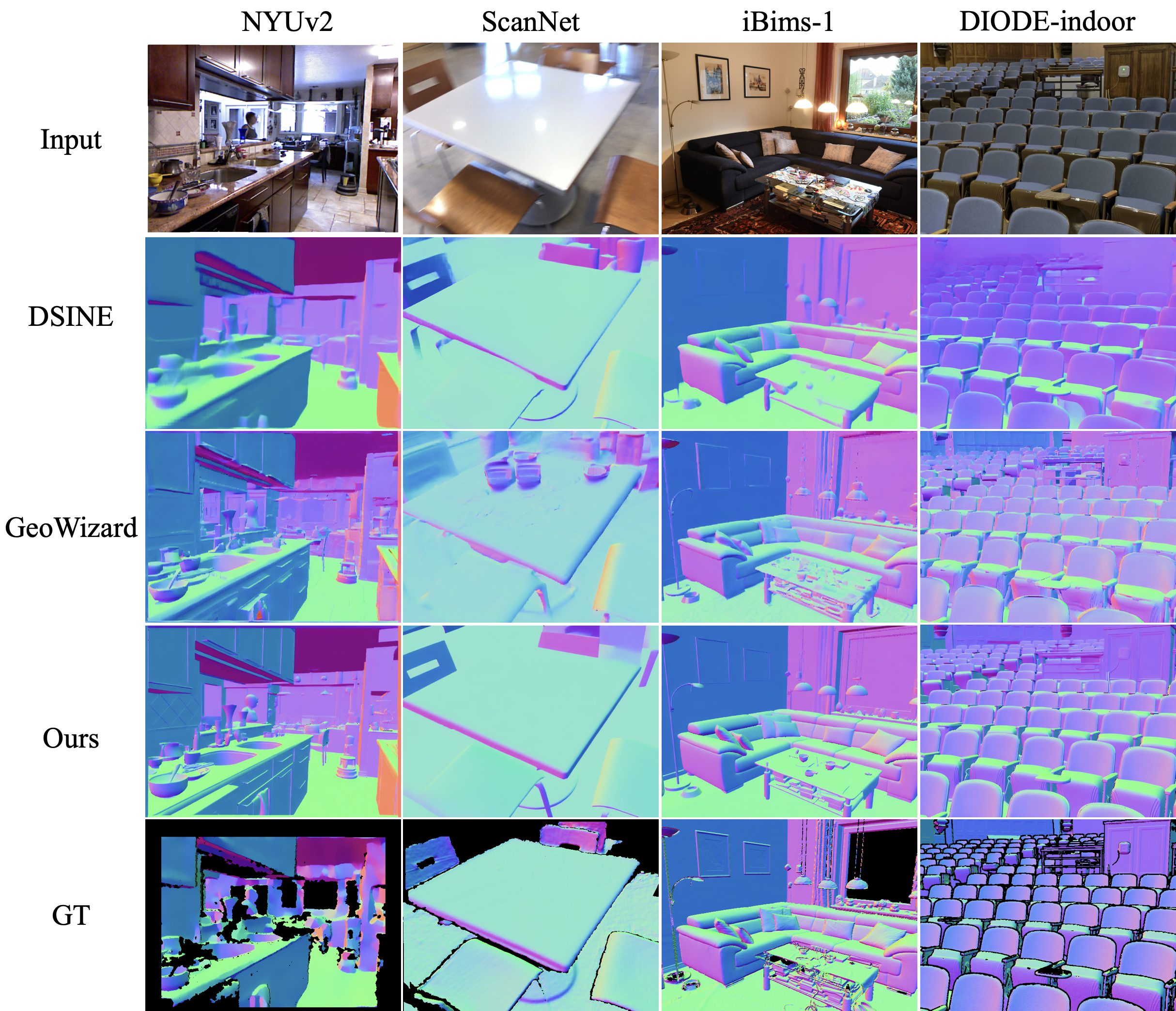
Figure 9. Qualitative comparison of different methods on NYUv2(Silberman et al., 2012), ScanNet(Dai et al., 2017), iBims-1(Koch et al., 2018), DIODE-indoor(Vasiljevic et al., 2019) datasets. StableNormal outperforms other related works in terms of accuracy and sharpness.

The testing data for evaluation includes the challenging DIODE-indoor (Vasiljevic et al., 2019), iBims (Koch et al., 2018), ScanNetV2 (Dai et al., 2017), and NYUv2 (Silberman et al., 2012) datasets. As presented in Tab. 2, our method achieves superior performance across iBims, ScanNetV2, and DIODE-indoor by a large margin. On NYUv2, our method is slightly inferior to DSINE. We argue that both Scannet and NYUV2 are captured using low-quality sensors, thus their GT normal are not accurate, which is also mentioned in GeoWizard (Fu et al., 2024b)). Figure 9 shows the qualitative comparisons on challenging scenarios, which demonstrates the accuracy and sharpness of StableNormal.

(a) Output Variance Analysis

(b) Inference Time Analysis

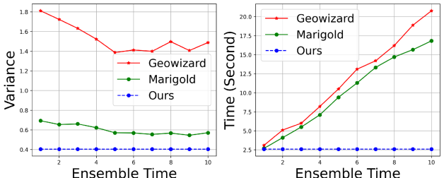
Ensemble Times

Ensemble Times

Figure 5. The comparison of output variance and inference time between our method, GeoWizard, and Marigold. The left plot shows the output variance over ensemble time, while the right plot displays the inference time (including ensembling). It is important to note that our method does not employ the ensemble strategy and only requires a single forward pass.

Figure 5 compares the inference variance and time between our method and GeoWizard on the DIODE-indoor dataset. Specifically, we estimate each image 10 times using different initialization seeds, allowing us to calculate the variance for each individual image. We then calculated the overall variance for each model by averaging these values across the entire dataset. As shown in Fig. 5 (a), GeoWizard employs an ensemble strategy to reduce the variance of the output. However, our approach significantly decreases the output variance (0.410 vs. 1.370) without introducing any ensemble strategies. Furthermore, the ensemble strategy compromises speed to achieve a lower variance. Figure 5 (b) shows that GeoWizard samples five times (approximately 10 seconds) to reach a variance of 1.370, while our method achieves a variance of 0.410 within 3 secs. The inference speed was tested on a single A100 GPU.

4.3. Ablation study

Table 3. Ablation Studies. Different cellcolors refers to best and 2nd-best.

	mean $\downarrow$	med$\downarrow$	$11.25^{\circ}$$\uparrow$	$22.5^{\circ}$$\uparrow$	$30^{\circ}$$\uparrow$
NYUv2 (Silberman et al., 2012)
Ours	19.707	10.527	53.042	75.889	81.723
YOSO Only	18.917	10.509	53.074	76.008	82.524
Ours w/o DINO	19.739	10.536	52.999	75.833	81.667
DSINE	18.610	9.885	56.132	76.944	82.606
SG-DRN + DSINE	19.869	10.548	52.952	75.738	81.575
ScanNet (Dai et al., 2017)
Ours	18.098	10.097	56.007	78.776	84.115
YOSO Only	17.679	9.860	57.220	78.823	84.331
Ours w/o DINO	19.326	11.626	48.115	77.438	83.575
DSINE	18.610	9.885	56.132	76.944	82.606
SG-DRN + DSINE	19.118	10.221	54.789	77.115	82.568
iBims-1 (Koch et al., 2018)
Ours	17.248	8.057	66.655	81.134	84.632
YOSO Only	17.695	8.431	63.635	80.212	84.034
Ours w/o DINO	18.234	8.875	62.172	80.417	84.347
DSINE	18.773	8.258	64.131	78.570	82.160
SG-DRN + DSINE	17.877	8.069	66.589	80.630	83.957
DIODE-indoor (Vasiljevic et al., 2019)
Ours	13.701	9.460	63.447	88.223	92.107
YOSO Only	17.122	13.787	32.950	83.385	89.884
Ours w/o DINO	15.611	11.912	45.801	86.563	91.843
DSINE	18.453	13.871	36.274	77.527	86.976
SG-DRN + DSINE	14.752	10.139	58.221	86.455	90.888

Table 4. Ablation study of the effectiveness of Shrinkage Regularizer. Best results are highlighted.

Ablation	Mean $\downarrow$	Med$\downarrow$	$11.25^{\circ}$$\uparrow$	$22.5^{\circ}$$\uparrow$	$30^{\circ}$$\uparrow$
DIODE-indoor (Vasiljevic et al., 2019)
w/o Shrinkage Regularizer	18.624	14.237	37.504	76.569	87.740
w/ Shrinkage Regularizer	17.122	13.787	32.950	83.385	89.884
iBims-1 (Koch et al., 2018)
w/o Shrinkage Regularizer	18.552	9.049	61.791	79.077	81.852
w/ Shrinkage Regularizer	17.695	8.431	63.635	80.212	84.034

We conduct ablation studies to analyze the contribution of each component in our framework across four datasets: NYUv2, ScanNet, iBims-1, and DIODE-indoor. Both quantitative and qualitative results are summarized in Table 3 and Fig. 6.

Ablation on SG-DRN. We first evaluated the refinement step – SG-DRN. We refer to the method without the refinement pipeline as YOSO Only. As shown in Table 3, there is a performance degradation on both the iBims-1 and DIODE-indoor datasets, highlighting the critical role of the SG-DRN refinement module in improving normal estimation accuracy. Notably, since NYUv2 and ScanNet feature smooth GT normals, and the prediction normals by YOSO Only are relatively smooth as well, the quantitative performance of YOSO Only even surpasses that of the full version with the refinement process. However, this is not the case when examining the qualitative results (see SupMat.’s Fig. R.3). Furthermore, we also evaluate the DSINE with SG-DRN module, refered as SG-DRN+DSINE, the results on DIODE-indoor and iBIMS-1 datasets also justify the effectiveness of multi-step refinement.

YOSO Normal Initialization. Next, we investigate the effect of the YOSO initialization . To do this, we tried an alternative to use the output of the DSINE method instead of our YOSO as the initialization, which is termed as SG-DRN $+$ DSINE. The results on the DIODE-indoor dataset reveal that using DSINE’s initialization leads to an increase in mean angle error from 13.701° to 18.453°. This verifies that the necessity of our YOSO initialization.

Ablation on Semantic feature extractor. There are alternatives for extracting semantic features. We denote the one replacing DINO extractor with a standard ResNet-50 backbone as Ours w/o DINO, with which, the performance decreases across all datasets, validating that the superiority of DINO visual representation to be the semantic guidance for normal estimation. The most significant drop is observed on the DIODE-Indoor dataset, where the mean angle error rises from 13.701° to 15.611°. Qualitative comparisons in Fig. 6 further verifies the usefulness of DINO features.

Effects of Shrinkage Regularizer. Table 4 illustrates that our proposed Shrinkage Regularizer can effectively mitigate the difficulty of learning many-to-one mapping, improving overall metrics on both DIODE-indoor and iBims-1 benchmark.

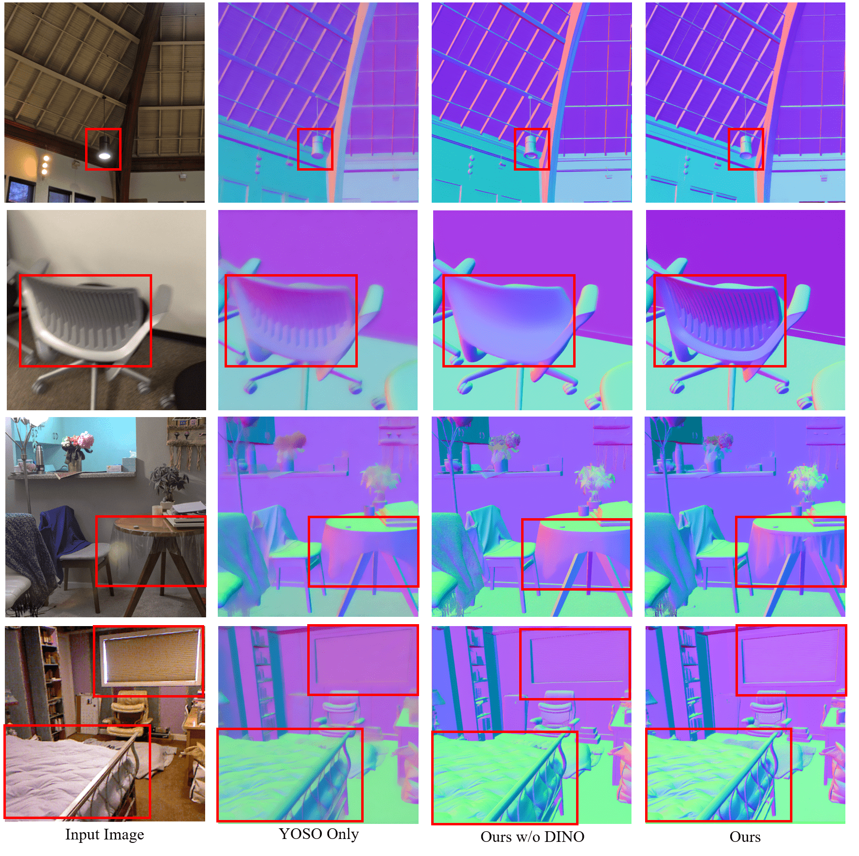
Figure 6. Qualitative Ablation Study. YOSO can produce relatively sharp surface normal estimations with only a single-step sampling; however, its results still lack sufficient details. After refinement by SG-DRN, the predicted surface normals become significantly sharper, as illustrated by the comparison between the third and fourth columns in the figure. This comparison highlights the impact of semantic features on SG-DRN’s performance. Specifically, the first row demonstrates how using DINO features assists the network in mitigating the effects of lighting on normal estimation. The second row indicates that DINO features enable effective structural modeling, enhancing the consistency of the normal output. Furthermore, the third row shows that DINO features improve the network’s ability to understand materials, e.g., plastic material.

5. Applications

5.1. Multi-view Surface Reconstruction

Accurate normal estimation is crucial for faithful surface reconstructions, especially for non-Lambertian surfaces (Fig. 7). We leverage our generated normal maps to regularize the surface reconstruction pipeline following 2DGS (Huang et al., 2024). Quantitative results on DTU (Table 1) show our method achieves the lowest mean Chamfer distance among compared techniques, highlighting the significant impact of our accurate normal estimates.

5.2. Monocular Surface Reconsturction

Our high-fidelity normal estimation also benefits monocular surface reconstruction via normal field integration, like Bilateral Normal Integration (BiNI) (Cao et al., 2022). We compare monocular geometric regularization from different methods on 80 DiLiGenT samples with ground-truth normals. Table 5 reports our method significantly improves Normal RMSE, Mean Angle Error (by  20%), and Depth Mean Angle Error over previous methods, demonstrating robust normal estimation across lighting conditions. Fig. 8 visualizes extracted mesh comparisons against GT and GeoWizard, showing our method faithfully recovers intricate geometric structures.

Table 5. Quantitative evaluation on the DiLiGenT (Shi et al., 2019) dataset for monocular surface reconsturction application. Different cellcolors refers to best, and 2nd-best.

Method	N-RMSE $\downarrow$	MAE $\downarrow$	D-RMSE $\downarrow$
DSINE(Bae and Davison, 2024)	0.50	22.53	0.0053
GeoWizard(Fu et al., 2024b)	0.49	24.51	0.0048
Ours	0.41	18.78	0.0044

5.3. Normal Enhancement

Recent generative AI advances enable 3D content creation by finetuning pre-trained 2D diffusion models to predict multi-view normal maps (Lu et al., 2024; Zheng et al., 2024; Qiu et al., 2024; Long et al., 2023), which are then fused into 3D models. However, existing methods produce low-resolution and over-smooth outputs lacking fine details. To improve it, we apply our method to Wonder3D (Long et al., 2023) to improve the detail of the generated multi-view normal maps and the resulting 3D shapes. We upsample the multi-view images using bilinear upsampling and the low-res normal maps to initialize $x_{t}$, leveraging their multi-view consistency. Our SG-DRN then refines the upsampled normal maps to recover finer details. Following Wonder3D (Long et al., 2023), we train a NeuS (Wang et al., 2021) per object using the refined normal maps and extract high-res meshes. Figure 10 shows our method significantly improves the detail of the generated 3D objects compared to the original one.

6. Conclusion

We present StableNormal, which tailors the diffusion priors for monocular normal estimation. Unlike prior diffusion-based works, we prioritize enhancing estimation stability by reducing inherent diffusion stochasticity. Our approach, a coarse-to-fine strategy, hinges on the belief that a reliable initial guess combined with a semantic-guided refinement process is crucial for balancing the “stability vs. sharpness” trade-off. This is validated by multiple indoor benchmarks, and various real-world applications (check our video for more details). Some failure cases are in SupMat.’s Appendix C. While our focus is on normal estimation, we believe our methodology and the identified trade-off will also benefit other related fields, including but not limited to depth estimation and various perception tasks (e.g., detection, segmentation, etc). To democratize this, we will make our code and models publicly available, only for research purpose.

 

Acknowledgments. We thank Guanying Chen and Zhen Liu for proofreading, Zhen Liu and Xu Cao for fruitful discussions.

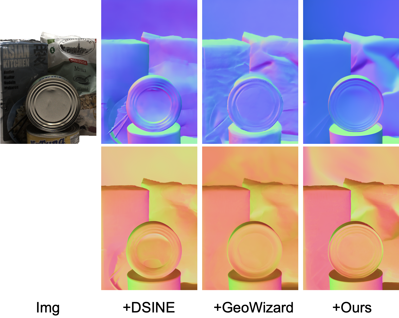
Figure 7. Qualitative comparison on DTU(Jensen et al., 2014)dataset. The first row displays the input images and estimated normal maps. The second row visualizes the rendered world-space normal maps after the reconstruction.

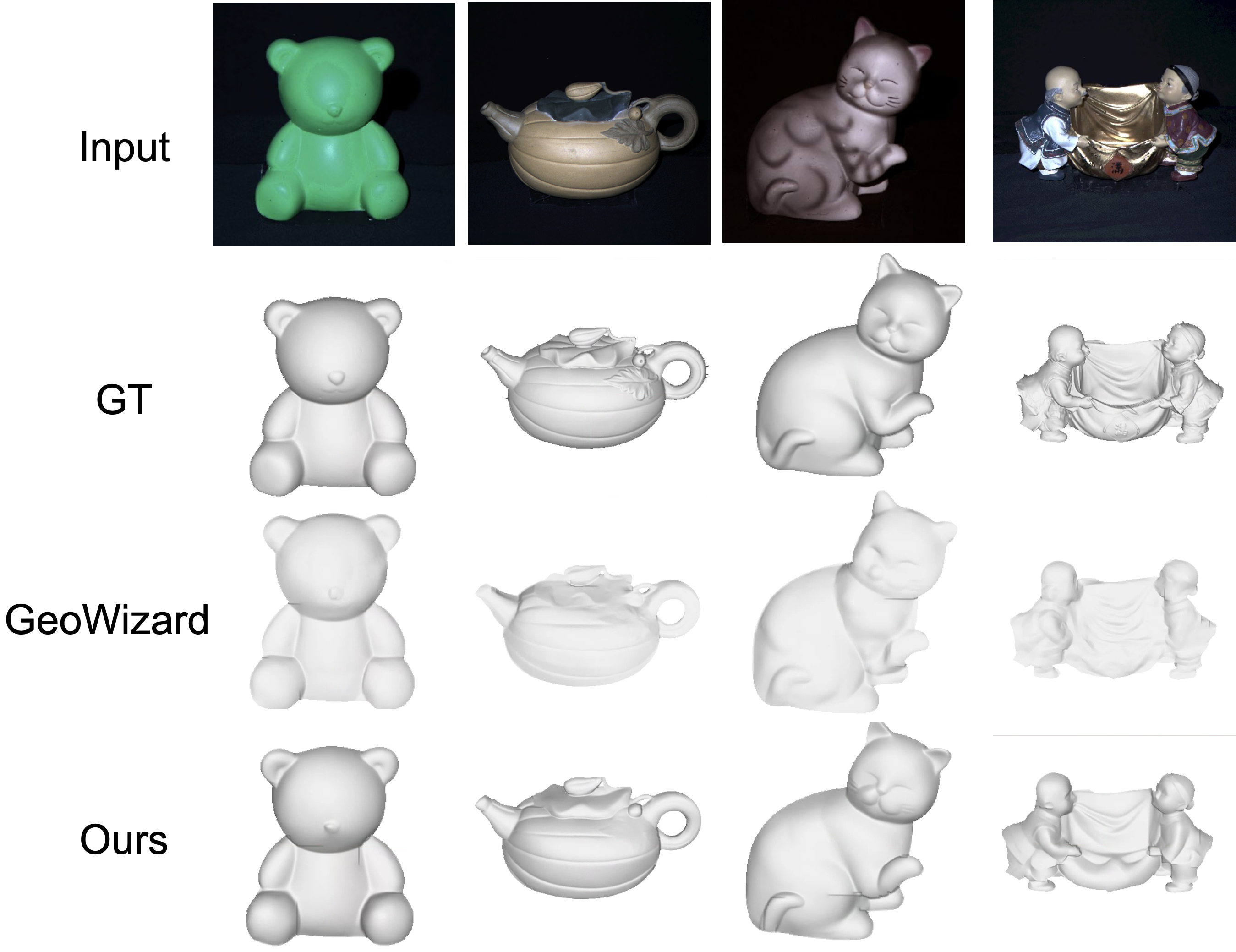
Figure 8. Qualitative comparison on DiLiGenT(Shi et al., 2019) dataset.

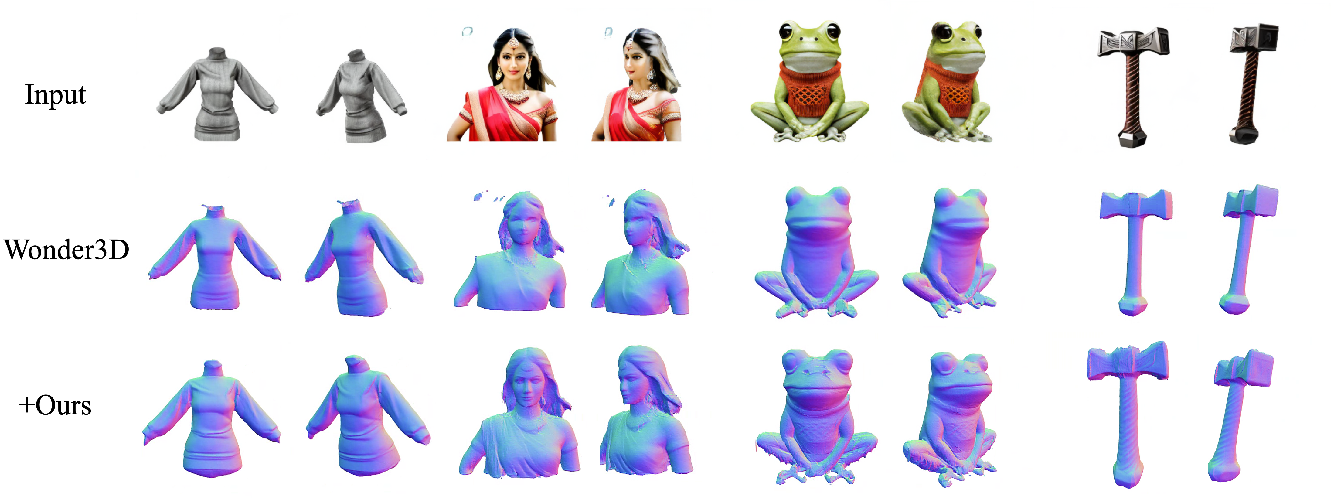
Figure 10. Comparison of geometric surface normals for different scenes. The surface normals are rendered from the reconstructed 3D mesh models.

Appendix A More details about implementation

We fine-tune the pre-trained Stable Diffusion V2.1 (Rombach et al., 2022b) using the AdamW optimizer(Loshchilov and Hutter, 2019) with a fixed learning rate of 3e-5. To enhance the robustness of our method against exposure, we incorporate exposure augmentation. Furthermore, we transform all input maps to the range [-1, 1] to align with the VAE’s expected input range. During training, we employ random crops with varying aspect ratios and pad the images to a fixed box resolution using black padding. Our training process involves two stages: first, we pre-train our network with a resolution of 512x512 using a batch size of 64 for around 20,000 steps. Subsequently, we fine-tune the model on a 768x768 resolution with a batch size of 32 for 10,000 steps. The entire training process takes approximately one day on four A100 GPUs. Notably, both YOSO and SG-DRN employ the same training strategy.

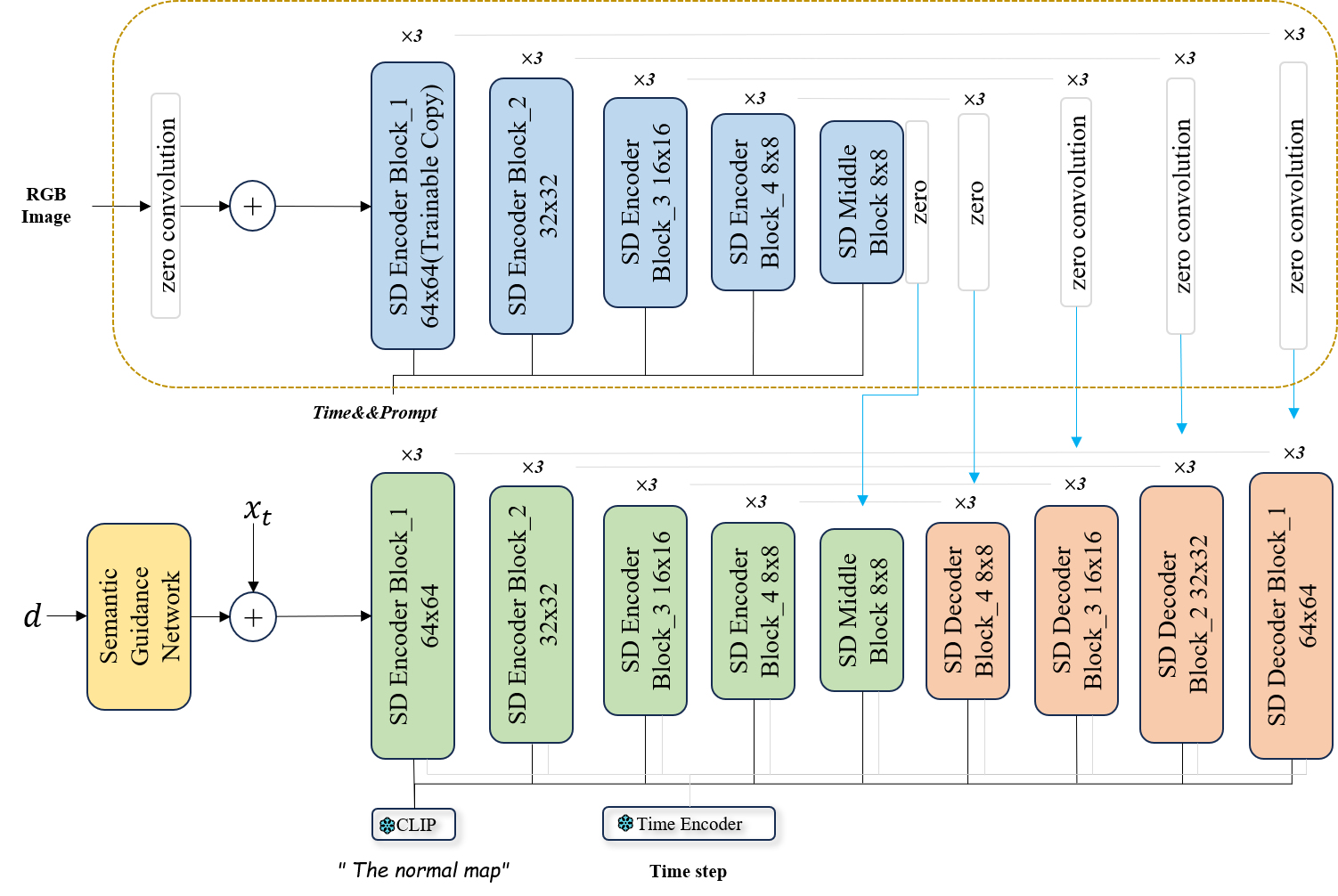
Figure R.1. The details of the architecture of our U-Net.

Appendix B The architecture of U-Net in both stages

Our structure maintains most building blocks of ControlNet (Zhang et al., 2023a) with several modifications for normal estimation(we show the second stage here). As depicted in Figure. R.1, we use a fixed text prompt “The Normal Map” in both the training and testing phases and add a semantic-guider network to encode DINO features. The encoded feature is further added with the output of the YOSO stage to act as input to the SG-DRN. The semantic guider is a simple stacking of 2D convolutions for obtain features, following by Featup (Fu et al., 2024a) and bi-linear interpolation to upsample their resolution to the same shape as the YOSO output.

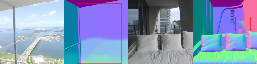
Figure R.2. Typical bad cases generated by StabelNormal.

Appendix C Failure Case

While StableNormal can produce sharp and stable normal estimation under most circumstances, it may also fail in some extreme cases like all data-driven methods. As depicted in Figure. R.2, StableNormal could partially output the normal of things behind the transparent objects(Left) and output a similar color(green) for plants in images(Right) regardless of the complex normal directions on the surface of plants. This is due to the inductive bias introduced by our training dataset(Lack of data including outdoor scenes and plants), which could be solved in the future by adding more simulating renderings.

Appendix D More qualitative analysis of YOSO

Although our method predicts sharper and more accurate normals compared to YOSO Only, the qualitative results appear worse than those of YOSO Only because the ground truth normal maps of both NYUv2 and ScanNet are smoother and less detailed (see Fig. R.3).

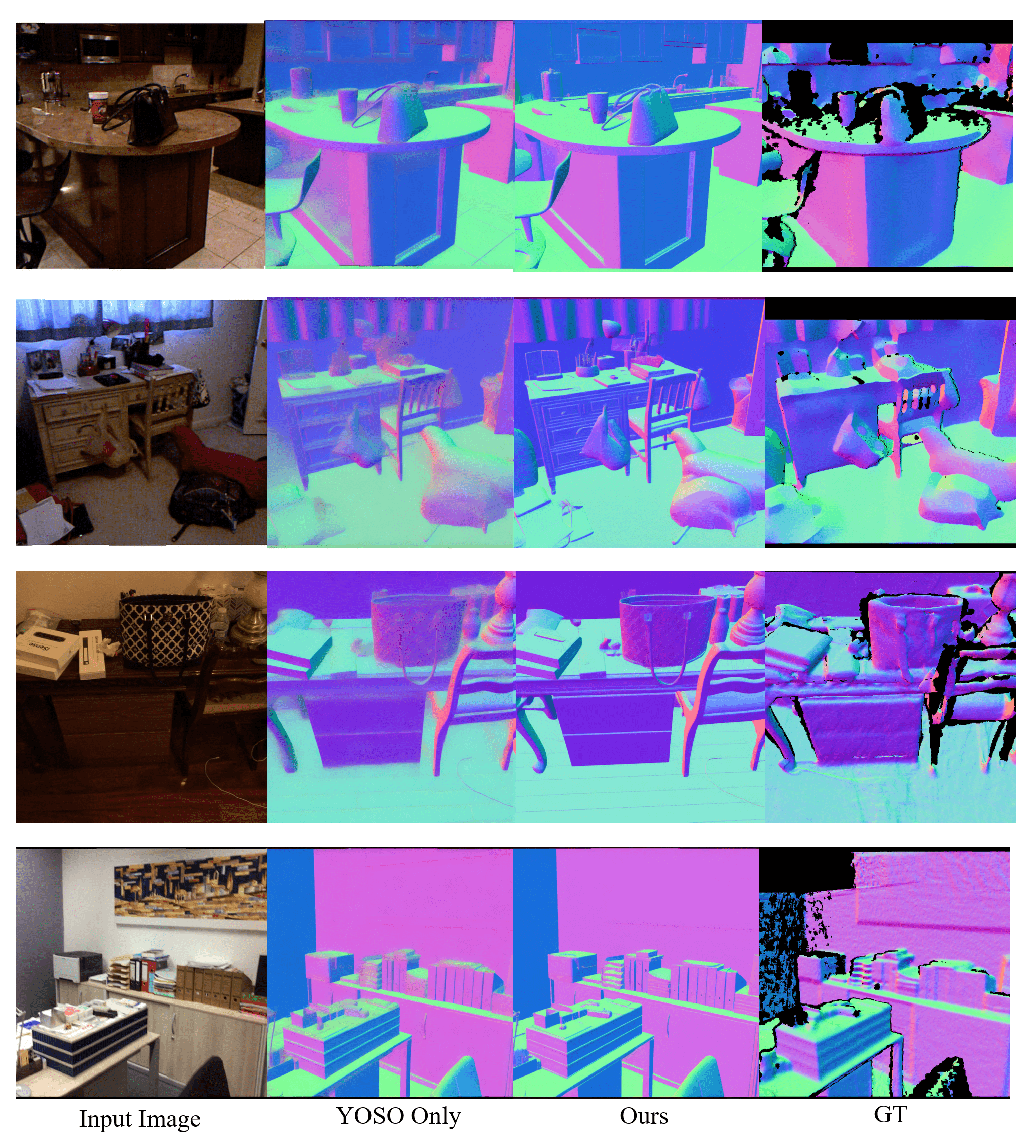
Figure R.3. The qualitative comparison results between YOSO Only and Ours on both NYUv2 and ScanNet dataset.

Appendix E More qualitative comparisons

We present more qualitative comparison results between GeoWizard (Fu et al., 2024b), DSINE (Bae and Davison, 2024), Marigold (Ke et al., 2024a), GenPercept (Xu et al., 2024) and StableNormal from Fig. R.4 to Fig. R.7.

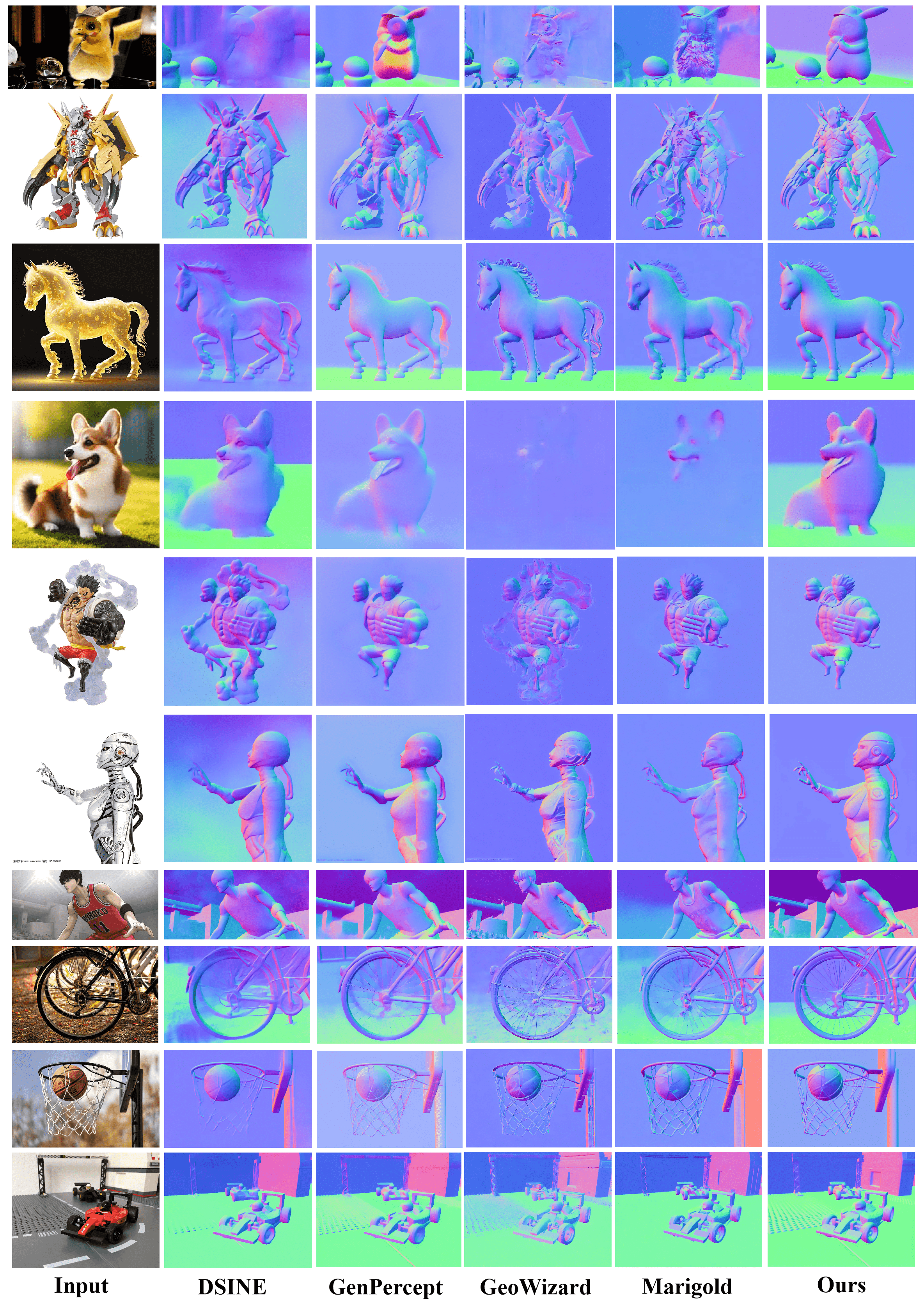
Figure R.4. More qualitative results (Part I). From the left to the right are results from DSINE (Bae and Davison, 2024), GenPercept (Xu et al., 2024), GeoWizard (Fu et al., 2024b), Marigold (Ke et al., 2024b) and StableNormal respectively.

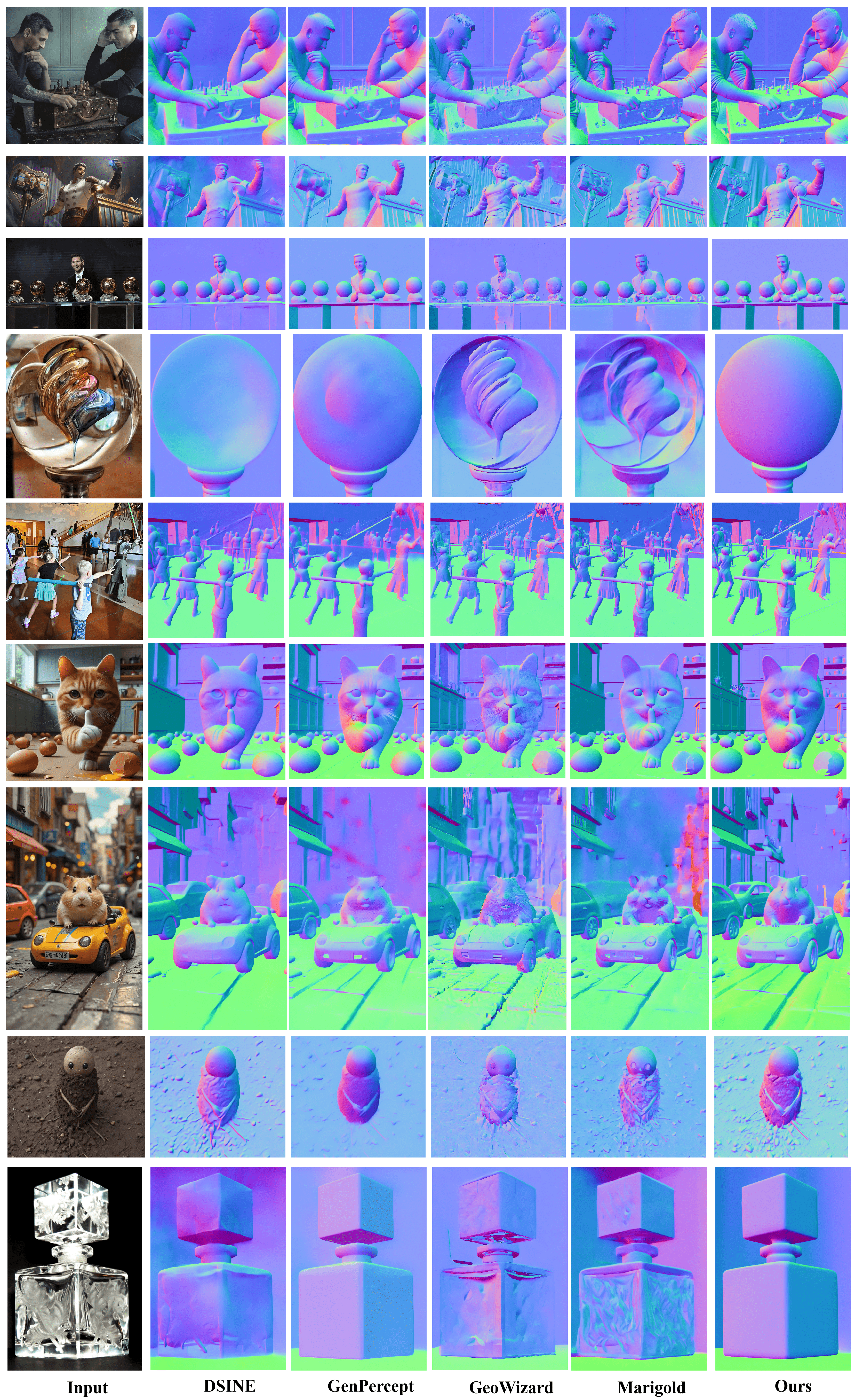
Figure R.5. More qualitative results (Part II). From the left to the right are results from DSINE (Bae and Davison, 2024), GenPercept (Xu et al., 2024), GeoWizard (Fu et al., 2024b), Marigold (Ke et al., 2024b) and StableNormal respectively.

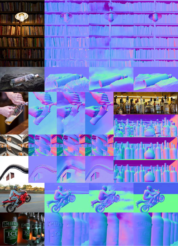
Figure R.6. More qualitative results (Part III). From the left to the right (the up to the bottom) are results from GeoWizard (Fu et al., 2024b), DSINE(Bae and Davison, 2024), and StableNormal respectively.

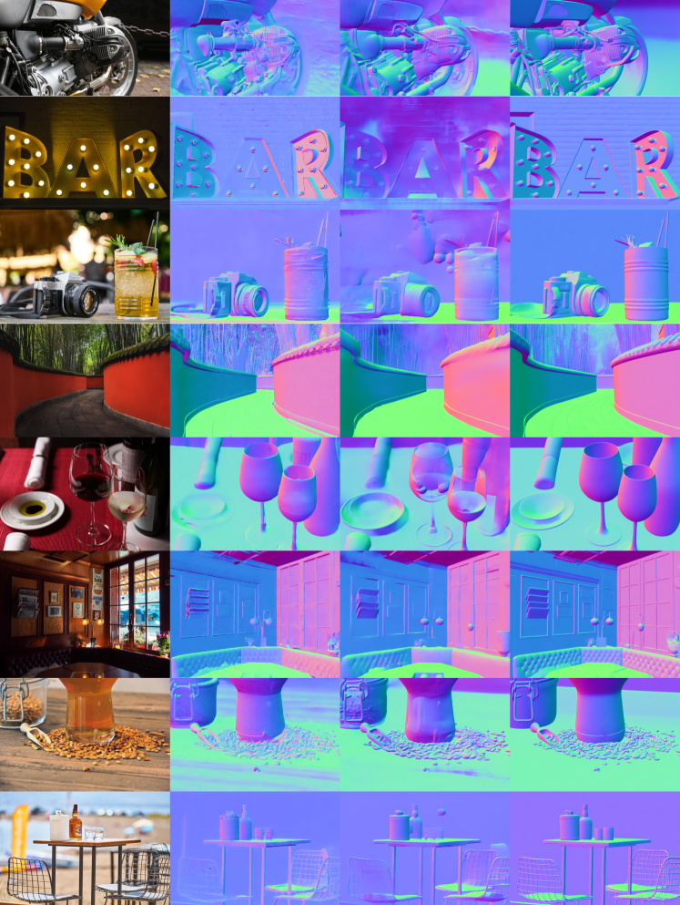
Figure R.7. More qualitative results (Part IV). From the left to the right are results from GeoWizard (Fu et al., 2024b), DSINE (Bae and Davison, 2024), and StableNormal respectively.

References

- (1)
- Bae et al. (2021) Gwangbin Bae, Ignas Budvytis, and Roberto Cipolla. 2021. Estimating and Exploiting the Aleatoric Uncertainty in Surface Normal Estimation. In 2021 IEEE/CVF International Conference on Computer Vision (ICCV). https://doi.org/10.1109/iccv48922.2021.01289
- Bae and Davison (2024) Gwangbin Bae and Andrew J. Davison. 2024. Rethinking Inductive Biases for Surface Normal Estimation. In IEEE/CVF Conference on Computer Vision and Pattern Recognition (CVPR).
- Bansal et al. (2016a) Aayush Bansal, Bryan Russell, and Abhinav Gupta. 2016a. Marr revisited: 2d-3d alignment via surface normal prediction. In Proceedings of the IEEE conference on computer vision and pattern recognition. 5965–5974.
- Bansal et al. (2016b) Aayush Bansal, Bryan Russell, and Abhinav Gupta. 2016b. Marr Revisited: 2D-3D Alignment via Surface Normal Prediction. In 2016 IEEE Conference on Computer Vision and Pattern Recognition (CVPR). https://doi.org/10.1109/cvpr.2016.642
- Bar et al. (2022) Amir Bar, Yossi Gandelsman, Trevor Darrell, Amir Globerson, and Alexei Efros. 2022. Visual prompting via image inpainting. Conference on Neural Information Processing Systems (NeurIPS) 35 (2022), 25005–25017.
- Baradad et al. (2023) Manel Baradad, Yuanzhen Li, Forrester Cole, Michael Rubinstein, Antonio Torralba, William T. Freeman, and Varun Jampani. 2023. Background Prompting for Improved Object Depth. arXiv:2306.05428 [cs.CV]
- Cao et al. (2022) Xu Cao, Hiroaki Santo, Boxin Shi, Fumio Okura, and Yasuyuki Matsushita. 2022. Bilateral normal integration. In European Conference on Computer Vision. Springer, 552–567.
- Dai et al. (2017) Angela Dai, Angel X. Chang, Manolis Savva, Maciej Halber, Thomas Funkhouser, and Matthias Nießner. 2017. ScanNet: Richly-annotated 3D Reconstructions of Indoor Scenes. arXiv:1702.04405 [cs.CV]
- Deitke et al. (2022) Matt Deitke, Dustin Schwenk, Jordi Salvador, Luca Weihs, Oscar Michel, Eli VanderBilt, Ludwig Schmidt, Kiana Ehsani, Aniruddha Kembhavi, and Ali Farhadi. 2022. Objaverse: A Universe of Annotated 3D Objects. arXiv preprint arXiv:2212.08051 (2022).
- Do et al. (2020) TienVan Do, Khiem Vuong, StergiosI. Roumeliotis, and HyunSoo Park. 2020. Surface Normal Estimation of Tilted Images via Spatial Rectifier. Cornell University - arXiv,Cornell University - arXiv (Jul 2020).
- Eftekhar et al. (2021) Ainaz Eftekhar, Alexander Sax, Jitendra Malik, and Amir Zamir. 2021. Omnidata: A scalable pipeline for making multi-task mid-level vision datasets from 3d scans. In Proceedings of the IEEE/CVF International Conference on Computer Vision. 10786–10796.
- Eigen and Fergus (2015a) David Eigen and Rob Fergus. 2015a. Predicting depth, surface normals and semantic labels with a common multi-scale convolutional architecture. In Proceedings of the IEEE international conference on computer vision. 2650–2658.
- Eigen and Fergus (2015b) David Eigen and Rob Fergus. 2015b. Predicting Depth, Surface Normals and Semantic Labels with a Common Multi-Scale Convolutional Architecture. In 2015 IEEE International Conference on Computer Vision (ICCV). https://doi.org/10.1109/iccv.2015.304
- Everaert et al. (2024) Martin Nicolas Everaert, Athanasios Fitsios, Marco Bocchio, Sami Arpa, Sabine Süsstrunk, and Radhakrishna Achanta. 2024. Exploiting the signal-leak bias in diffusion models. In Proceedings of the IEEE/CVF Winter Conference on Applications of Computer Vision. 4025–4034.
- Fouhey et al. (2013a) David F Fouhey, Abhinav Gupta, and Martial Hebert. 2013a. Data-driven 3D primitives for single image understanding. In Proceedings of the IEEE International Conference on Computer Vision. 3392–3399.
- Fouhey et al. (2013b) David F. Fouhey, Abhinav Gupta, and Martial Hebert. 2013b. Data-Driven 3D Primitives for Single Image Understanding. In 2013 IEEE International Conference on Computer Vision. https://doi.org/10.1109/iccv.2013.421
- Fouhey et al. (2014) David Ford Fouhey, Abhinav Gupta, and Martial Hebert. 2014. Unfolding an Indoor Origami World. 687–702. https://doi.org/10.1007/978-3-319-10599-4_44
- Fu et al. (2024a) Stephanie Fu, Mark Hamilton, Laura E. Brandt, Axel Feldmann, Zhoutong Zhang, and William T. Freeman. 2024a. FeatUp: A Model-Agnostic Framework for Features at Any Resolution. In The Twelfth International Conference on Learning Representations. https://openreview.net/forum?id=GkJiNn2QDF
- Fu et al. (2024b) Xiao Fu, Wei Yin, Mu Hu, Kaixuan Wang, Yuexin Ma, Ping Tan, Shaojie Shen, Dahua Lin, and Xiaoxiao Long. 2024b. GeoWizard: Unleashing the Diffusion Priors for 3D Geometry Estimation from a Single Image. arxiv (2024).
- Ho et al. (2020) Jonathan Ho, Ajay Jain, and Pieter Abbeel. 2020. Denoising diffusion probabilistic models. Advances in neural information processing systems 33 (2020), 6840–6851.
- Hoiem et al. (2005) Derek Hoiem, Alexei A. Efros, and Martial Hebert. 2005. Automatic photo pop-up. ACM Transactions on Graphics (Jul 2005), 577–584. https://doi.org/10.1145/1073204.1073232
- Hoiem et al. (2007) Derek Hoiem, Alexei A. Efros, and Martial Hebert. 2007. Recovering Surface Layout from an Image. International Journal of Computer Vision (Jul 2007), 151–172. https://doi.org/10.1007/s11263-006-0031-y
- Huang et al. (2024) Binbin Huang, Zehao Yu, Anpei Chen, Andreas Geiger, and Shenghua Gao. 2024. 2D Gaussian Splatting for Geometrically Accurate Radiance Fields. In SIGGRAPH 2024 Conference Papers. Association for Computing Machinery. https://doi.org/10.1145/3641519.3657428
- Huang et al. (2019) Jingwei Huang, Yichao Zhou, Thomas Funkhouser, and LeonidasJ. Guibas. 2019. FrameNet: Learning Local Canonical Frames of 3D Surfaces from a Single RGB Image. Cornell University - arXiv,Cornell University - arXiv (Mar 2019).
- Jensen et al. (2014) Rasmus Ramsbøl Jensen, A. Dahl, George Vogiatzis, Engil Tola, and Henrik Aanæs. 2014. Large Scale Multi-view Stereopsis Evaluation. 2014 IEEE Conference on Computer Vision and Pattern Recognition (2014), 406–413.
- Ji et al. (2023) Yuanfeng Ji, Zhe Chen, Enze Xie, Lanqing Hong, Xihui Liu, Zhaoqiang Liu, Tong Lu, Zhenguo Li, and Ping Luo. 2023. Ddp: Diffusion model for dense visual prediction. In Proceedings of the IEEE/CVF International Conference on Computer Vision. 21741–21752.
- Ke et al. (2024a) Bingxin Ke, Anton Obukhov, Shengyu Huang, Nando Metzger, Rodrigo Caye Daudt, and Konrad Schindler. 2024a. Repurposing Diffusion-Based Image Generators for Monocular Depth Estimation. In Computer Vision and Pattern Recognition (CVPR).
- Ke et al. (2024b) Bingxin Ke, Anton Obukhov, Shengyu Huang, Nando Metzger, Rodrigo Caye Daudt, and Konrad Schindler. 2024b. Repurposing Diffusion-Based Image Generators for Monocular Depth Estimation. In Proceedings of the IEEE/CVF Conference on Computer Vision and Pattern Recognition (CVPR).
- Koch et al. (2018) Tobias Koch, Lukas Liebel, Friedrich Fraundorfer, and Marco Körner. 2018. Evaluation of CNN-based Single-Image Depth Estimation Methods. arXiv:1805.01328 [cs.CV]
- Kocsis et al. (2024) Peter Kocsis, Vincent Sitzmann, and Matthias Nießner. 2024. Intrinsic Image Diffusion for Single-view Material Estimation. In Computer Vision and Pattern Recognition (CVPR).
- Ladický et al. (2014) L’ubor Ladický, Bernhard Zeisl, and Marc Pollefeys. 2014. Discriminatively Trained Dense Surface Normal Estimation. 468–484. https://doi.org/10.1007/978-3-319-10602-1_31
- Lasinger et al. (2019) Katrin Lasinger, René Ranftl, Konrad Schindler, and Vladlen Koltun. 2019. Towards robust monocular depth estimation: Mixing datasets for zero-shot cross-dataset transfer. arXiv preprint arXiv:1907.01341 (2019).
- Li et al. (2023b) Alexander C Li, Mihir Prabhudesai, Shivam Duggal, Ellis Brown, and Deepak Pathak. 2023b. Your diffusion model is secretly a zero-shot classifier. In International Conference on Computer Vision (ICCV). 2206–2217.
- Li et al. (2023a) Yixuan Li, Lihan Jiang, Linning Xu, Yuanbo Xiangli, Zhenzhi Wang, Dahua Lin, and Bo Dai. 2023a. Matrixcity: A large-scale city dataset for city-scale neural rendering and beyond. In Proceedings of the IEEE/CVF International Conference on Computer Vision. 3205–3215.
- Li et al. (2023c) Ziyi Li, Qinye Zhou, Xiaoyun Zhang, Ya Zhang, Yanfeng Wang, and Weidi Xie. 2023c. Open-vocabulary object segmentation with diffusion models. In International Conference on Computer Vision (ICCV). 7667–7676.
- Liao et al. (2019) Shuai Liao, Efstratios Gavves, and CeesG.M. Snoek. 2019. Spherical Regression: Learning Viewpoints, Surface Normals and 3D Rotations on n-Spheres. Cornell University - arXiv,Cornell University - arXiv (Apr 2019).
- Liu et al. (2023) Xian Liu, Jian Ren, Aliaksandr Siarohin, Ivan Skorokhodov, Yanyu Li, Dahua Lin, Xihui Liu, Ziwei Liu, and Sergey Tulyakov. 2023. Hyperhuman: Hyper-realistic human generation with latent structural diffusion. arXiv preprint arXiv:2310.08579 (2023).
- Long et al. (2023) Xiaoxiao Long, Yuan-Chen Guo, Cheng Lin, Yuan Liu, Zhiyang Dou, Lingjie Liu, Yuexin Ma, Song-Hai Zhang, Marc Habermann, Christian Theobalt, et al. 2023. Wonder3d: Single image to 3d using cross-domain diffusion. (2023).
- Loshchilov and Hutter (2019) Ilya Loshchilov and Frank Hutter. 2019. Decoupled Weight Decay Regularization. arXiv:1711.05101 [cs.LG]
- Lu et al. (2024) Yuanxun Lu, Jingyang Zhang, Shiwei Li, Tian Fang, David McKinnon, Yanghai Tsin, Long Quan, Xun Cao, and Yao Yao. 2024. Direct2.5: Diverse Text-to-3D Generation via Multi-view 2.5D Diffusion. arXiv:2311.15980 [cs.CV]
- Niklaus et al. (2019) Simon Niklaus, Long Mai, Jimei Yang, and Feng Liu. 2019. 3D Ken Burns Effect from a Single Image. ACM Transactions on Graphics 38, 6 (2019), 184:1–184:15.
- Oquab et al. (2024) Maxime Oquab, Timothée Darcet, Théo Moutakanni, Huy Vo, Marc Szafraniec, Vasil Khalidov, Pierre Fernandez, Daniel Haziza, Francisco Massa, Alaaeldin El-Nouby, Mahmoud Assran, Nicolas Ballas, Wojciech Galuba, Russell Howes, Po-Yao Huang, Shang-Wen Li, Ishan Misra, Michael Rabbat, Vasu Sharma, Gabriel Synnaeve, Hu Xu, Hervé Jegou, Julien Mairal, Patrick Labatut, Armand Joulin, and Piotr Bojanowski. 2024. DINOv2: Learning Robust Visual Features without Supervision. arXiv:2304.07193 [cs.CV]
- Peebles and Xie (2022) William Peebles and Saining Xie. 2022. Scalable Diffusion Models with Transformers.
- Poole et al. (2023) Ben Poole, Ajay Jain, Jonathan T Barron, and Ben Mildenhall. 2023. Dreamfusion: Text-to-3d using 2d diffusion. International Conference on Learning Representations (ICLR) (2023).
- Qi et al. (2018) Xiaojuan Qi, Renjie Liao, Zhengzhe Liu, Raquel Urtasun, and Jiaya Jia. 2018. GeoNet: Geometric Neural Network for Joint Depth and Surface Normal Estimation. In 2018 IEEE/CVF Conference on Computer Vision and Pattern Recognition. https://doi.org/10.1109/cvpr.2018.00037
- Qi et al. (2022) Xiaojuan Qi, Zhengzhe Liu, Renjie Liao, Philip H. S. Torr, Raquel Urtasun, and Jiaya Jia. 2022. GeoNet++: Iterative Geometric Neural Network with Edge-Aware Refinement for Joint Depth and Surface Normal Estimation. IEEE Transactions on Pattern Analysis and Machine Intelligence (Feb 2022), 969–984. https://doi.org/10.1109/tpami.2020.3020800
- Qiu et al. (2024) Lingteng Qiu, Guanying Chen, Xiaodong Gu, Qi Zuo, Mutian Xu, Yushuang Wu, Weihao Yuan, Zilong Dong, Liefeng Bo, and Xiaoguang Han. 2024. Richdreamer: A generalizable normal-depth diffusion model for detail richness in text-to-3d. In Proceedings of the IEEE/CVF Conference on Computer Vision and Pattern Recognition. 9914–9925.
- Radford et al. (2021) Alec Radford, Jong Wook Kim, Chris Hallacy, Aditya Ramesh, Gabriel Goh, Sandhini Agarwal, Girish Sastry, Amanda Askell, Pamela Mishkin, Jack Clark, et al. 2021. Learning transferable visual models from natural language supervision. In International conference on machine learning.
- Ranftl et al. (2021a) René Ranftl, Alexey Bochkovskiy, and Vladlen Koltun. 2021a. Vision transformers for dense prediction. In Proceedings of the IEEE/CVF international conference on computer vision. 12179–12188.
- Ranftl et al. (2021b) Rene Ranftl, Alexey Bochkovskiy, and Vladlen Koltun. 2021b. Vision Transformers for Dense Prediction. International Conference on Computer Vision,International Conference on Computer Vision (Jan 2021).
- Roberts et al. (2021) Mike Roberts, Jason Ramapuram, Anurag Ranjan, Atulit Kumar, Miguel Angel Bautista, Nathan Paczan, Russ Webb, and Joshua M. Susskind. 2021. Hypersim: A Photorealistic Synthetic Dataset for Holistic Indoor Scene Understanding. arXiv:2011.02523 [cs.CV]
- Rombach et al. (2021) Robin Rombach, Andreas Blattmann, Dominik Lorenz, Patrick Esser, and Björn Ommer. 2021. High-Resolution Image Synthesis with Latent Diffusion Models. arXiv:2112.10752 [cs.CV]
- Rombach et al. (2022a) Robin Rombach, Andreas Blattmann, Dominik Lorenz, Patrick Esser, and Björn Ommer. 2022a. High-resolution image synthesis with latent diffusion models. In Computer Vision and Pattern Recognition (CVPR). 10684–10695.
- Rombach et al. (2022b) Robin Rombach, Andreas Blattmann, Dominik Lorenz, Patrick Esser, and Björn Ommer. 2022b. High-Resolution Image Synthesis With Latent Diffusion Models. In Proceedings of the IEEE/CVF Conference on Computer Vision and Pattern Recognition (CVPR). 10684–10695.
- Ronneberger et al. (2015) Olaf Ronneberger, Philipp Fischer, and Thomas Brox. 2015. U-Net: Convolutional Networks for Biomedical Image Segmentation. Lecture Notes in Computer Science,Lecture Notes in Computer Science (Jan 2015).
- Schuhmann et al. (2022) Christoph Schuhmann, Romain Beaumont, Richard Vencu, Cade Gordon, Ross Wightman, Mehdi Cherti, Theo Coombes, Aarush Katta, Clayton Mullis, Mitchell Wortsman, et al. 2022. Laion-5b: An open large-scale dataset for training next generation image-text models. Advances in Neural Information Processing Systems 35 (2022), 25278–25294.
- Shi et al. (2019) Boxin Shi, Zhipeng Mo, Zhe Wu, Dinglong Duan, Sai-Kit Yeung, and Ping Tan. 2019. A Benchmark Dataset and Evaluation for Non-Lambertian and Uncalibrated Photometric Stereo. IEEE Transactions on Pattern Analysis and Machine Intelligence 41 (2019), 271–284. https://api.semanticscholar.org/CorpusID:156683
- Silberman et al. (2012) Nathan Silberman, Derek Hoiem, Pushmeet Kohli, and Rob Fergus. 2012. Indoor Segmentation and Support Inference from RGBD Images. In European Conference on Computer Vision.
- Song et al. (2020) Jiaming Song, Chenlin Meng, and Stefano Ermon. 2020. Denoising diffusion implicit models. arXiv preprint arXiv:2010.02502 (2020).
- Straub et al. (2019) Julian Straub, Thomas Whelan, Lingni Ma, Yufan Chen, Erik Wijmans, Simon Green, Jakob J Engel, Raul Mur-Artal, Carl Ren, Shobhit Verma, et al. 2019. The Replica dataset: A digital replica of indoor spaces. arXiv preprint arXiv:1906.05797 (2019).
- Tian et al. (2024) Junjiao Tian, Lavisha Aggarwal, Andrea Colaco, Zsolt Kira, and Mar Gonzalez-Franco. 2024. Diffuse, Attend, and Segment: Unsupervised Zero-Shot Segmentation using Stable Diffusion. Computer Vision and Pattern Recognition (CVPR) (2024).
- Vasiljevic et al. (2019) Igor Vasiljevic, Nick Kolkin, Shanyi Zhang, Ruotian Luo, Haochen Wang, Falcon Z. Dai, Andrea F. Daniele, Mohammadreza Mostajabi, Steven Basart, Matthew R. Walter, and Gregory Shakhnarovich. 2019. DIODE: A Dense Indoor and Outdoor DEpth Dataset. arXiv:1908.00463 [cs.CV]
- Wang et al. (2021) Peng Wang, Lingjie Liu, Yuan Liu, Christian Theobalt, Taku Komura, and Wenping Wang. 2021. NeuS: Learning Neural Implicit Surfaces by Volume Rendering for Multi-view Reconstruction. Conference on Neural Information Processing Systems (NeurIPS) (2021).
- Wang et al. (2016) Peng Wang, Xiaohui Shen, Bryan Russell, Scott Cohen, Brian Price, and AlanL. Yuille. 2016. SURGE: surface regularized geometry estimation from a single image. Neural Information Processing Systems,Neural Information Processing Systems (Dec 2016).
- Wang et al. (2020) Rui Wang, David Geraghty, Kevin Matzen, Richard Szeliski, and Jan-Michael Frahm. 2020. VPLNet: Deep Single View Normal Estimation With Vanishing Points and Lines. In 2020 IEEE/CVF Conference on Computer Vision and Pattern Recognition (CVPR). https://doi.org/10.1109/cvpr42600.2020.00077
- Wang et al. (2015a) Xiaolong Wang, David Fouhey, and Abhinav Gupta. 2015a. Designing deep networks for surface normal estimation. In Proceedings of the IEEE conference on computer vision and pattern recognition. 539–547.
- Wang et al. (2015b) Xiaolong Wang, David F. Fouhey, and Abhinav Gupta. 2015b. Designing Deep Networks for Surface Normal Estimation. In 2015 IEEE Conference on Computer Vision and Pattern Recognition (CVPR). https://doi.org/10.1109/cvpr.2015.7298652
- Wang et al. (2023) Zhendong Wang, Yifan Jiang, Yadong Lu, Pengcheng He, Weizhu Chen, Zhangyang Wang, Mingyuan Zhou, et al. 2023. In-context learning unlocked for diffusion models. Conference on Neural Information Processing Systems (NeurIPS) 36 (2023), 8542–8562.
- Xu et al. (2024) Guangkai Xu, Yongtao Ge, Mingyu Liu, Chengxiang Fan, Kangyang Xie, Zhiyue Zhao, Hao Chen, and Chunhua Shen. 2024. Diffusion Models Trained with Large Data Are Transferable Visual Models. arXiv preprint arXiv:2403.06090 (2024).
- Zhang et al. (2023a) Lvmin Zhang, Anyi Rao, and Maneesh Agrawala. 2023a. Adding Conditional Control to Text-to-Image Diffusion Models. In IEEE International Conference on Computer Vision (ICCV).
- Zhang et al. (2023b) Shiwei Zhang, Jiayu Wang, Yingya Zhang, Kang Zhao, Hangjie Yuan, Zhiwu Qin, Xiang Wang, Deli Zhao, and Jingren Zhou. 2023b. I2vgen-xl: High-quality image-to-video synthesis via cascaded diffusion models. arXiv preprint arXiv:2311.04145 (2023).
- Zhang et al. (2019) Zhenyu Zhang, Zhen Cui, Chunyan Xu, Yan Yan, Nicu Sebe, and Jian Yang. 2019. Pattern-Affinitive Propagation across Depth, Surface Normal and Semantic Segmentation. In 2019 IEEE/CVF Conference on Computer Vision and Pattern Recognition (CVPR). https://doi.org/10.1109/cvpr.2019.00423
- Zhao et al. (2023) Wenliang Zhao, Yongming Rao, Zuyan Liu, Benlin Liu, Jie Zhou, and Jiwen Lu. 2023. Unleashing text-to-image diffusion models for visual perception. In Proceedings of the IEEE/CVF International Conference on Computer Vision. 5729–5739.
- Zheng et al. (2024) Xin-Yang Zheng, Hao Pan, Yu-Xiao Guo, Xin Tong, and Yang Liu. 2024. MVD2: Efficient Multiview 3D Reconstruction for Multiview Diffusion. arXiv:2402.14253 [cs.CV]