Can Quantum Computers Do Nothing?
Abstract
Quantum computing platforms are subject to contradictory engineering requirements: qubits must be protected from mutual interactions when idling (‘doing nothing’), and strongly interacting when in operation. If idling qubits are not sufficiently protected, information can ‘leak’ into neighbouring qubits, become non-locally distributed, and ultimately inaccessible. Candidate solutions to this dilemma include patterning-enhanced many-body localization, dynamical decoupling, and active error correction. However, no information-theoretic protocol exists to actually quantify this information loss due to internal dynamics in a similar way to e.g. SPAM errors or dephasing times. In this work, we develop a scalable, flexible, device non-specific protocol for quantifying this bitwise idle information loss based on the exploitation of tools from quantum information theory. We implement this protocol in over 3500 experiments carried out across 4 months (Dec 2023 - Mar 2024) on IBM’s entire Falcon 5.11 series of processors. After accounting for other sources of error, and extrapolating results via a scaling analysis in shot count to zero shot noise, we detect idle information leakage to a high degree of statistical significance. This work thus provides a firm quantitative foundation from which the protection-operation dilemma can be investigated and ultimately resolved.
I Introduction
Quantum computing is a new paradigm of computation based on the exploitation of quantum phenomena which promises frontier impacts on global energy, health, materials science, and technological innovation [1, 2]. With the firm advent of the noisy intermediate-scale quantum (NISQ) era in the form of accessible quantum processors containing some tens to hundreds of qubits [3, 4, 5, 6], out-of-the-box error mitigation [7], and the nascent implementation of simple error correction [8, 9, 10], this new paradigm is now being mapped out comprehensively. However, far from their conceptualization as ideal systems, real quantum computers are intrinsically programmable many-body quantum systems with complicated internal dynamics exposed to stray interactions and thermal fluctuations (Fig. 1(a-b) schematically show idealized and realistic ‘empty’ circuits respectively) [11]. The precise control of these complex many-body physical systems is ultimately the fundamental problem of quantum computing.
This problem is encapsulated by the ‘protection-operation dilemma’ wherein qubits need to be coupled and decoupled from each other at different times during the same computation [12]. When not in active operation (‘doing nothing’), idling qubits should be well protected from mutual interactions with other qubits in the device. However, multi-qubit operation require strong mutual interactions such that entanglement and correlations can be generated between the active qubits quickly. Both of these processes should also be resistant to environmental decoherence, which typically reduces to the requirement that computations should be completed as quickly as possible. This generates contradicting engineering requirements: qubits should be decoupled when idling, but strongly coupled when necessary for computation. The two main ways this contradiction is resolved are (i) many-body localizing the qubits through spatial disorder and only bringing neighbouring qubits into resonance during gate operations (ii) rapidly tuning the mutual interactions in-situ to actively couple and decouple qubits during runtime [12, 13, 14]. The potential breakdown of the former resolution has been addressed in detail by recent works which find that current-generation superconducting quantum computers may enter chaotic regimes during operation; calling into question how well protected qubits in these devices actually are [15, 16, 17]. The latter poses a complicated engineering problem that may induce higher order or time-dependent effects which are not yet fully understood. Idle information leakage can also be reduced by active error correction or dynamical decoupling, but these introduce formidable engineering problems and additional gate-based errors and complexity respectively [18, 19].
Inspired by the burgeoning many-body perspective on quantum computation, we exploit tools from many-body physics and quantum information theory to address a critical question underlying the entire protection-operation dilemma: can the information loss induced by multi-qubit dynamics during idling be quantified in a similar way to e.g. readout errors or dephasing times? In this work we address this question directly by presenting and experimentally implementing a protocol for quantifying idle information loss. This protocol, developed and discussed in Section II, leverages the Holevo quantity to accurately quantify information loss, is device non-specific, scalable, and can be easily run during computational downtime. We experimentally implement the protocol in Section III across the entire range of Falcon 5.11 series of IBM’s quantum devices 111IBM has recently discontinued this particular series, but the protocol is not device-specific.. After accounting for other sources of error, we identify a small but measurable amount of information leakage to a high degree of statistical significance. Our accurate quantification of the actual informational impact of many-body effects in real devices represents a decisive step towards identifying and measuring idle information loss in future quantum devices. This result also provides a firm quantitative foundation from which the protection-operation dilemma can be further interrogated and resolved.
II Quantifying Internal Information Leakage
Information lost whilst idling due to the native dynamics of a device manifests as the spreading of information that is initially localized. Information initially localized to a single qubit moves coherently into the rest of the system and is distributed non-locally. Thus the basic premise of our protocol is to monitor both a target qubit from which information may leak out, and a complementary set of qubits into which information may have flowed. This is shown schematically in Fig. 1(c) for two types of complementary qubit set: nearest-neigbour (blue) and random (orange). The basic mathematical object we use to characterize the amount of information lost is the Holevo quantity [21]: an import from quantum information theory that quantifies the amount of classical information that a channel and an ensemble of messages (an alphabet) can carry [22]. We discuss the Holevo quantity in detail in Section II.1 for the interested reader.
The protocol in an ideal system, with no other sources of error, is discussed in detail in Section II.2. The protocol involves initializing a target qubit in one of two message states and which encode a classical bit. By calculating the Holevo quantity both over the target qubit alone , and over a complementary set of qubits which includes the target qubit , we can quantify how much extra information we get about the initial classical binary message by looking at non-local degrees of freedom. If the difference between these two Holevo quantities is finite, then information has leaked out of the target qubit. In Section II.3 we address other sources of error, and discuss how to unravel them from true information leakage due to internal dynamics. The major issue we identify is shot noise which can artificially induce a significant signature of information loss. We address this issue in Section III by exploiting central limiting behaviour, and present an ansatz for extrapolating information loss at zero shot noise during our experimental implementation of the protocol.
We remark on two major elements of the protocol which impose constraints on the types of device to which it is applicable. The platform must be capable of (i) full state tomography on at least two qubits (a target qubit, and at least one other qubit in the device) (ii) initializing the target qubit in two definite states. We assume nothing about the microscopic features of the native physics of a device except that (iii) the dynamics are in some way local: qubits are assumed to couple more strongly to their neighbours than qubits further away in an array. This means we can look at nearest-neighbour qubits and random qubits, both of which are equally susceptible to single-qubit errors and shot noise but are not equally sensitive to information leakage affecting a fixed target qubit.
II.1 The Holevo Quantity
The Holevo quantity over an alphabet and channel quantifies - in bits - the accessible information that is carried by the protocol wherein states are selected with probability and transmitted through the channel [21, 22]. The Holevo quantity is given by
| (1) |
The Holevo quantity has been used to characterize information in many-body systems before, and is a natural quantity with which to investigate information loss [23, 24, 25, 26]. We critically note that the initial space and final space are not generally identical. Consider e.g. a protocol which prepares a target qubit in a specific state, but performs measurements on the combined final state of the target qubit and its nearest-neighbours.
When maximized over all possible input alphabets , gives the maximum classical capacity of the channel . However, this maximization is often not possible in practice: the precise nature of a device’s underlying Hamiltonian, and thus of the channel , is subject to debate - and the Hamiltonian parameters are subject to random fluctuations and drift. However, quantum computing platforms should approximately realize identities on idling qubits. Thus it is reliable to define an alphabet of equi-probable , pure, and orthogonal messages which cover the state space (this choice saturates when is the identity channel).
We now discuss another important property of the Holevo quantity which becomes critically relevant when we try to account for shot noise in Section III. It is intuitively appropriate to consider as encapsulating the notion of distinguishability. Direct inspection the form of reveals that an alphabet of pure states which are not all mutually orthogonal will cause the first term of Eq. 1 to fail to saturate, resulting in a low value of . Conversely, an alphabet of states which are close to maximally mixed states will saturate the first term, but also saturate the second - resulting in a low value for overall. Thus the Holevo quantity can be understood as a careful balancing act between the mixedness of the source (first term) and purity of the individual messages (second term) which together capture distinguishability. This may seem like a pedantic point, but it becomes critical when accounting for the effect of shot noise. Whilst the Holevo quantity is monotonically decreasing under the implementation of a CPTP channel, shot noise can not be represented as such, and can thus artificially increase the Holevo quantity. More precisely, shot noise is realised as random contributions to elements of the final density matrices . These contributions can increase distinguishability but does not actually increase the amount of information that the channel can bear. This effect becomes exacerbated in the case that the dimension of the initial space is smaller than the dimension of the final space. If , there are more elements in density matrices drawn from the final space, and thus shot noise introduces more differences between output density matrices.
In the context of this article (and in the absence of shot noise, which we address separately), the Holevo quantity quantifies how much information we can access about the initial state of a qubit given access to it and access to some other subset of qubits on the device. If no information has coherently leaked out of the target qubit, then access to some other region should not give us additional information about its initial state.
II.2 Protocol for Quantifying Idle Information Loss
We now leverage Holevo quantities computed over two subsets of qubits on a device into protocol which quantifies the information lost to other qubits during idling. We first introduce the Holevo quantities and , respectively computed on the final reduced density matrices (i) of the target qubit alone , and (ii) of the target qubit and a complementary set of qubits in the array . Note here that , and thus by the monotonicity of the Holevo quantity under the partial trace:
| (2) |
with equality only when information is fully localized to the target qubit, or when and information has completely left the final space. Since the Holevo quantity yields the average number of bits of information that can be transmitted by messages passed through the channel, can also be interpreted as the extra bits of information we can access about the initial state of the target qubit given access to the complementary qubits . In ideal systems without shot noise or other sources of error suffices to identify and quantify information loss due to information leakage. Finite indicates that some information has left the target qubit in a coherent fashion, and is distributed non-locally: i.e. that the device can’t ‘do nothing’ perfectly, even in ideal conditions. The protocol in full is as follows:
-
1.
Initialize every qubit except the target qubit in an arbitrary state (we take pure separable product states of the logical single-qubit states throughout).
-
2.
Initialize the target qubit in the state .
-
3.
Wait for a fixed period of time (we measure immediately to address the ‘best case’ scenario with minimal information leakage such that is the readout time of the device) 222 is arbitrary in principle, and can be tuned to address different regimes or properties of a device. Taking to be e.g. fifty two-qubit gate times could give us a good indicator of the total information leakage during a complete computation..
-
4.
Perform full state tomography on the combined state of the target and complementary qubits (the subscript denotes that this state is conditioned upon the initial state, prepared in step 2).
-
5.
Repeat from step 1, with the target qubit initialized in the state , generating the state .
-
6.
Process the states into a sample value for .
-
7.
Check the condition .
-
8.
(Optional, to address noise) Repeat from step 1 for a large number of samples to build up statistics for .
II.3 Unravelling Information Leakage from Other Sources of Error
Unravelling information leakage from other sources is, in principle, a serious operational issue. As we discussed in Section II.1, shot noise may artificially increase distinguishability. Moreover, other sources of error may artificially increase the difference , which is not subject to the same monotonicity conditions as the Holevo quantity alone. In essence, can be non-zero in realistic systems even if information is fully localized to the target qubit. To deal with this we benchmark our results on nearest-neighbour qubits against random (non nearest-neighbour) qubits in the array , whilst keeping the target qubit fixed. Both of these sets of complementary qubits should, when averaged over a large number of samples - be equally affected by e.g. shot noise, SPAM errors, and environmentally-induced decoherence. However, the randomly selected qubits should bear much less information about the initial state of ; and thus they can serve as a benchmark for all other sources of error in the device. Nevertheless, we choose to carry out our experiments at very short timescales, two orders of magnitude less than the dephasing times of the devices we use, to mitigate the effect of the environment as much as possible. Our protocol does not make use of any gates in its implementation, and thus gate errors are vacuously irrelevant. We implement these benchmarking procedures in Section III and ultimately find that shot noise is the dominant contribution to in the system of interest. We suggest, but can not prove, that channels comprised of a linear combination of single-qubit processes can not systematically increase ; as such single-qubit processes can not systematically transfer information from to .
We first invoke the assumption that the underlying dynamics are, in a sense, local, and that the idea of ‘nearest-neighbours’ is thus well-defined. In such systems, information should flow from the target qubit to its nearest-neighbours, and then through them to more distant qubits in the array. For a fixed target qubit , we can then define two types of complementary sets of qubits: corresponding to the plaquette of the nearest-neighbours of , and corresponding to the target qubit and randomly selected (excluding nearest-neighbour) qubits in the array. Since and both contain the same number of qubits they should, after averaging, be equally susceptible to single-qubit errors and shot noise (see Appendix B for a detailed discussion on the origin of this shot noise in IBM devices). In an ideal system without other errors or shot noise should be a strict inequality (except at very late times where the information becomes fully delocalized). Individual samples may violate this inequality, but since both and are equally susceptible to all other sources of noise, these effects should cancel out after averaging over a large number of samples. We thus relax this condition to a statistical inequality
| (3) |
that should hold in the presence of non-trivial information leakage. Moreover, Eq. 3 can be easily realized as the alternative hypothesis for significance testing; which we do in Section III.
This inequality can be extended more formally by suggesting an ansatz form for as follows:
| (4) |
Which is a function of the excess accessible information , artificial information due to shot noise , and the shot count . We can aggregate statistics at different shot counts, perform a scaling analysis in , and extrapolate as . We develop just such an ansatz based on our experimental data in Section III. This also formalizes the intuitive notion of both the sets and of complementary qubits being ‘equally susceptible’ shot noise. We say that both are ‘equally susceptible’ to shot noise if after fitting. With shot noise mitigated, the difference then gives us the amount of information which has leaked from the target qubit into its neighbours.
In actual experiment (see Section III), we find exactly, supporting our previous assertion that other single-qubit sources of error can not systematically transfer information to distant regions of the device. This indicates that alone suffices to determine the amount of idle information loss in future experiments.
III Experimental Results and a Quantification of Idle Information Loss on IBM Devices
The experimental implementation of our protocol was carried out on the 27-qubit Falcon 5.11 series of IBM’s quantum computing devices; the architecture of such devices is shown in Fig. 1(c). We incorporate two additional steps into the general protocol given in Section II.2: (i) we only select target qubits with the highest possible coordination number , which should yield the strongest signatures of idle information loss. And (ii) in step 1 of the protocol, we also simultaneously randomize over target qubits subject to the coordination constraint, and the Falcon 5.11 devices ibm_algiers, ibm_cairo, ibm_hanoi, and ibmq_kolkata themselves. This corresponds to the generation of statistics for which are device agnostic - i.e. the user is interested only in running their computation job on a 27-qubit Falcon 5.11 device, and doesn’t care about which specific device to which their jobs are assigned. We performed readout immediately after state preparation, such that the wait time in step 3 of the protocol was just the readout time of the given device (between 700ns and 900ns). This minimizes the effect of the environment, as these readout times are several orders of magnitude lower than typical T1 and T2 times. This also means that our results represent the best case scenario, and can not be improved by e.g. dynamical decoupling, as such processes are not possible during readout. Due to the existence of shot noise, the resulting density matrices after state tomography can have negative eigenvalues. We use a maximum-likelihood reconstruction method to rephysicalize the density matrices before post-processing [28]. A detailed discussion of the tomographic process is given in Appendix B, and the maximum-likelihood reconstruction of aphysical density matrices is discussed in Appendix C.
As discussed in Section II.2, we consider both nearest-neigbour and random sets of complementary qubits for each target qubit, and carry out separate collections of experiments for each at a range of different shot counts . The number of samples for all shot counts on both nearest-neighbour plaquettes and random qubits is summarized in Table 2 in Appendix B. All in all, our analysis of the Falcon 5.11 series involves the results of over 3500 experiments taken across four months (Dec 2023 - Mar 2024), and represents a broad-spectrum comprehensive investigation of idle information loss on these devices. As the runtime increases proportionally with the shot count, most of this time was spent collating results for higher shot count samples; thus a direct comparison where statistics are compared for lots of low shot count samples, is likely the best approach for characterizing idle information loss on IBM devices in the future.
III.1 Results and Analysis
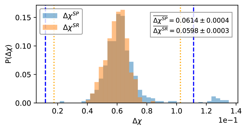
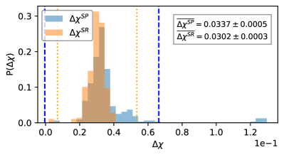
The experimentally determined statistics of and for 1209 total samples across all devices are shown in Fig. 2. The shot count for both was fixed at the standard value of . Both take a normally distributed form within certain limits, with exhibiting an additional small bump in the range . Were this bump due to any of the other processes discussed: decoherence, SPAM errors, shot noise, we would expect bumps to also appear in the statistics of . As this bump is not present in the statistics of , it stands to reason that this is strictly due to some target qubits coupling strongly to their nearest-neighbours. Moreover, we identify a bump in the statistics of at larger shot counts at the exact same position (see Appendix A), evidencing a true signature of idle information loss. The samples that form this bump can be justifiably interpreted as ‘bad qubits’ which have hybridized with their nearest-neighbours to such an extent that information leakage is dominating other sources of error. Over of the information about the initial state of such a qubit is stored non-locally.
A more subtle feature of Fig. 2 is that the statistics of show a thicker tail at larger values than , suggesting that the inequality Eq. 3 is satisfied even when these bad qubits are excluded. To quantify this difference, we first filter the statistics for outliers by simple box-filtering according to the condition [29, 30],
| (5) |
where we have introduced the subscript to denote individual samples of . Q1 and Q3 are the first and third quartiles of the full sample statistics respectively, and IQR is their inter-quartile range. Conservative filtration typically takes , whilst corresponds to no filtering at all. We take throughout as this both reliably contains the large Gaussian part of the distributions, and also excludes the bad qubit bump in the statistics of . We superimpose the boundaries of the box defined by Eq. 5 on Fig. 2 as dashed blue lines for and a dotted orange line for 333It is thus interesting to point out that we can thus invoke as a tuning parameter which defines precisely what is meant by a ‘bad qubit’. The part of the distribution to the right of the box defined by can inform us of the probability that any given qubit will be a ‘bad’ one up to a certain informational tolerance. In cases where the entire device is required to complete a computation, or bad qubits are not identified and excluded before runtime, this probability could be used to place bounds on ultimate ruin: wherein said computation fails completely. We defer this topic to future study.. After filtering, we can compute the means and standard errors in the means of the resulting datasets, which are displayed in the inset of Fig. 2. The results satisfy Eq. 3, and provide a clear ‘smoking gun’ for idle information loss in the investigated devices. More formally, we carried out a one-tailed Welch’s t-test with null hypothesis and alternative hypothesis Eq. 3. This yields a -value of (corresponding to a -value of ) which implies that the inequality holds to a high degree of statistical significance. We perform similar tests at a range of shot counts , the resulting -values and corresponding -values of which are summarized in Table 1. These results indicate that can be rejected to a very high degree of statistical significance, and thus that true signatures of idle information loss have been detected, across all investigated shot counts.
| Shot Count | -value | -value |
|---|---|---|
| 4000 | ||
| 8000 | ||
| 16000 | ||
| 32000 | ||
| 64000 |
III.2 Scaling analysis
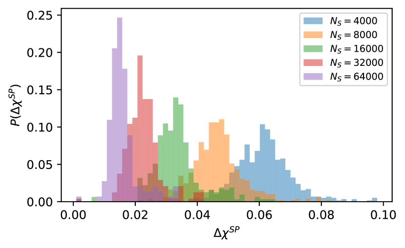
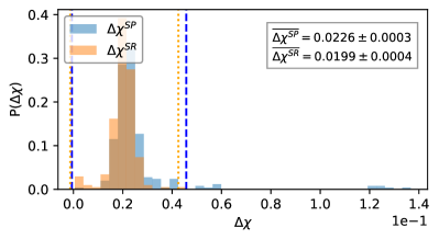
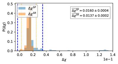
We now interrogate the effect of shot noise more rigorously by investigating how the statistics and mean values change as we vary the number of shots . This will form the basis of developing an ansatz of the form of Eq. 4 with which a scaling analysis can be carried out. The results of this investigation are shown in Fig. 3 which shows the statistics of after filtering as a function of shot count . The resulting distributions still appear normally distributed, but drift to lower mean values with smaller variances as is increased. Interestingly, the mean value of falls by a factor of every time is doubled. This is further evidence that shot noise, which should follow central limiting behaviour and scale as , is completely dominating the effects of idle information loss. We formalize this intuition by suggesting the simple ansatz
| (6) |
which incorporates both a flat information leakage and a term which captures the distinguishability introduced by shot noise . Essentially, can be interpreted as the number of additional bits of information we can retrieve about the initial state of the target qubit given access to the other qubits in the complementary set in the zero shot noise limit .
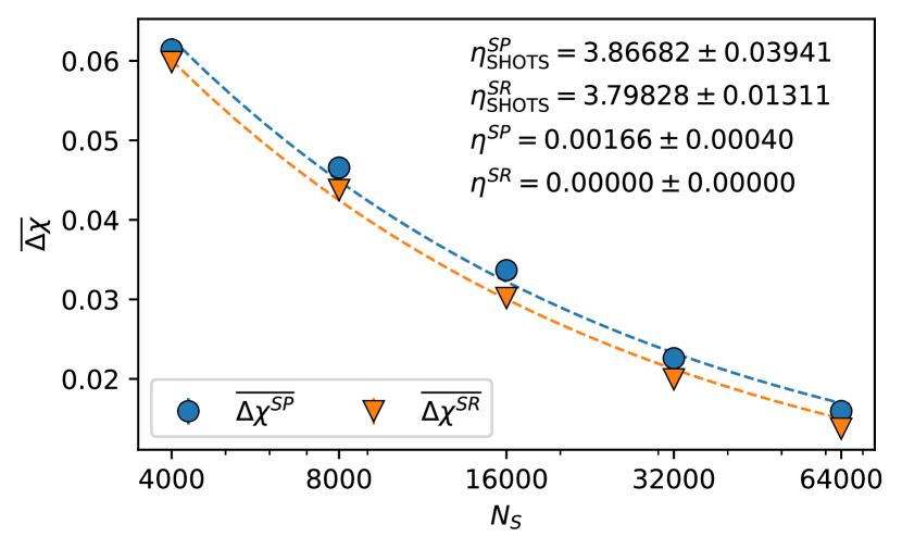
We present a fit of the mean values of the distributions (after filtering) of Fig. 3 to the ansatz of Eq. 6 in Fig. 4, where we find very good agreement between the data and our ansatz. We also present a fitting for filtered statistics as a benchmark. The fitting procedure allows us to extrapolate values for and , which are shown for both and in the inset text of Fig. 4. Standard errors on these extrapolated values are determined by a simple bootstrapping scheme in which each of the data points are randomly drawn from normal distributions determined by their respective means and standard deviations. These extrapolated values reveal that, as expected, both nearest-neighbour plaquettes and randomly selected qubits are equally affected by shot noise . However, the underlying idle information loss saturates to a low but finite value for nearest-neighbour plaquettes, and exactly to zero (to five decimal places) for randomly selected qubits. This evidences the conjecture made in Section II.3 that the single-qubit processes that lead to e.g. SPAM errors and decoherence have no systematic effect on , and that we can treat as a true zero shot noise quantification of idle information leakage. Ultimately, the excess information gained by having access to the joint state when compared to yields, on average, an additional bits of information about the target qubit . This is a low value, but it represents a direct quantification of the impact of idle information loss, and a fundamental limit on how well qubits in the Falcon 5.11 series of devices can perform.
IV Conclusions
The foremost result of this article is a protocol exploiting the Holevo quantity from quantum information theory. This protocol provides a flexible, scalable, device non-specific solution to the burgeoning problem of quantifying idle information leakage in quantum computing platforms. Sufficient degradation in single-qubit protection could destroy the ability of a device to actually carry out quantum computations as information propagates, and our protocol serves as a direct quantification of the information lost (in bits) to this effect. A central component of our protocol is simply waiting, i.e. implementing the empty circuit; and it can thus be easily run during downtime with minimal oversight, replacing otherwise wasted time with a valuable characterization of errors in the computing platform.
The secondary result of this article is the experimental implementation of our protocol on 3500 samples carried out across four months on all four of IBM’s Falcon 5.11 series of devices. The results of this analysis reveal (i) that a measurable amount of information about the state of any given qubit is leaking out during idling and (ii) the existence of ‘bad qubits’ which leak over of a classical bit of information into their immediate surroundings. The ‘smoking gun’ of idle information loss takes the form of a statistical inequality which accounts for the effects of e.g. SPAM errors, decoherence, and shot noise. We find this inequality to be satisfied to remarkably high degrees of statistical significance at all shot counts. We also determine an ansatz from which exact idle information loss at zero shot noise can be extrapolated. The results of this extrapolation indicate that, after filtering for bad qubits, approximately of the information stored locally is lost to idle information loss during a single readout time. This is a low, and but crucially non-zero, value which represents a fundamental limit on how well the Falcon 5.11 series of devices can perform.
Overall, our results indicate that, in contrast to what has been suggested in literature [15], unwanted many-body effects are not a significant concern in current-generation IBM devices when compared to shot noise; with the exception of occasional bad qubits. However, the main finding of our work is that a measurable albeit small amount of information is already being lost in these systems and we can study this accurately with our method. This should allow us to systematically understand the impact of innovating technologies on the protection-operation dilemma. The near future of quantum computing promises dramatic scale-ups of system sizes, nascent error correcting hardware, novel approaches to localizing information, and fledgling fault-tolerance. Our work provides a flexible, powerful, scalable protocol to quantify idle information loss in all these settings. This represents a decisive step towards addressing the threat many-body effects pose to high-fidelity idling, and thus to the long-term large-scale stability of generic quantum computing platforms.
V Acknowledgements
A.N.-K. would like to thank S. Bose, C. Turner, C. Berke, and O. Dial for fruitful discussions at preliminary research stages. A.N.-K. sincerely thanks S. Shaikh and C. Bleger for their support. N.K. would like to give thanks to the QuSys group for discussions throughout the project, and also to G. García-Pérez, S. Filippov, and E. Borrelli for giving feedback and useful references. J.G. is supported by a SFI- Royal Society University Research Fellowship and is grateful to IBM Ireland and Microsoft Ireland for generous financial support.
References
- Altman et al. [2021] E. Altman, K. R. Brown, G. Carleo, L. D. Carr, E. Demler, C. Chin, B. DeMarco, S. E. Economou, M. A. Eriksson, K.-M. C. Fu, M. Greiner, K. R. Hazzard, R. G. Hulet, A. J. Kollár, B. L. Lev, M. D. Lukin, R. Ma, X. Mi, S. Misra, C. Monroe, K. Murch, Z. Nazario, K.-K. Ni, A. C. Potter, P. Roushan, M. Saffman, M. Schleier-Smith, I. Siddiqi, R. Simmonds, M. Singh, I. Spielman, K. Temme, D. S. Weiss, J. Vučković, V. Vuletić, J. Ye, and M. Zwierlein, Quantum simulators: Architectures and opportunities, PRX Quantum 2, 017003 (2021).
- Bravyi et al. [2022] S. Bravyi, O. Dial, J. M. Gambetta, D. Gil, and Z. Nazario, The future of quantum computing with superconducting qubits, Journal of Applied Physics 132, 160902 (2022), https://pubs.aip.org/aip/jap/article-pdf/doi/10.1063/5.0082975/19808793/160902_1_online.pdf .
- Preskill [2018] J. Preskill, Quantum Computing in the NISQ era and beyond, Quantum 2, 79 (2018).
- Arute et al. [2019] F. Arute, K. Arya, R. Babbush, D. Bacon, J. C. Bardin, R. Barends, R. Biswas, S. Boixo, F. G. Brandao, D. A. Buell, et al., Quantum supremacy using a programmable superconducting processor, Nature 574, 505 (2019).
- Chow et al. [2021] J. Chow, O. Dial, and J. Gambetta, Ibm quantum breaks the 100-qubit processor barrier, IBM Research Blog 2 (2021).
- Kim et al. [2023] Y. Kim, A. Eddins, S. Anand, K. X. Wei, E. Van Den Berg, S. Rosenblatt, H. Nayfeh, Y. Wu, M. Zaletel, K. Temme, et al., Evidence for the utility of quantum computing before fault tolerance, Nature 618, 500 (2023).
- Van Den Berg et al. [2023] E. Van Den Berg, Z. K. Minev, A. Kandala, and K. Temme, Probabilistic error cancellation with sparse pauli–lindblad models on noisy quantum processors, Nature Physics 19, 1116 (2023).
- Takeda et al. [2022] K. Takeda, A. Noiri, T. Nakajima, T. Kobayashi, and S. Tarucha, Quantum error correction with silicon spin qubits, Nature 608, 682 (2022).
- AI [2023] G. Q. AI, Suppressing quantum errors by scaling a surface code logical qubit, Nature 614, 676 (2023).
- Xu et al. [2024a] Q. Xu, J. P. Bonilla Ataides, C. A. Pattison, N. Raveendran, D. Bluvstein, J. Wurtz, B. Vasić, M. D. Lukin, L. Jiang, and H. Zhou, Constant-overhead fault-tolerant quantum computation with reconfigurable atom arrays, Nature Physics , 1 (2024a).
- Xu et al. [2024b] X. Xu, C. Vignes, M. H. Ansari, J. Martinis, et al., Lattice hamiltonians and stray interactions within quantum processors, arXiv preprint arXiv:2402.09145 (2024b).
- Silveri and Orell [2022] M. Silveri and T. Orell, Many-qubit protection-operation dilemma from the perspective of many-body localization, nature communications 13, 5825 (2022).
- Qian et al. [2023] P. Qian, H.-Z. Xu, P. Zhao, X. Li, and D. E. Liu, Mitigating crosstalk and residual coupling errors in superconducting quantum processors using many-body localization, arXiv preprint arXiv:2310.06618 (2023).
- Varvelis and DiVincenzo [2024] E. Varvelis and D. P. DiVincenzo, Perturbative analysis of quasiperiodic patterning of transmon quantum computers: Enhancement of many-body localization, Phys. Rev. B 109, 144201 (2024).
- Berke et al. [2022] C. Berke, E. Varvelis, S. Trebst, A. Altland, and D. P. DiVincenzo, Transmon platform for quantum computing challenged by chaotic fluctuations, Nature communications 13, 2495 (2022).
- Börner et al. [2023] S.-D. Börner, C. Berke, D. P. DiVincenzo, S. Trebst, and A. Altland, Classical chaos in quantum computers, arXiv preprint arXiv:2304.14435 (2023).
- Basilewitsch et al. [2024] D. Basilewitsch, S.-D. Börner, C. Berke, A. Altland, S. Trebst, and C. P. Koch, Chaotic fluctuations in a universal set of transmon qubit gates, arXiv preprint arXiv:2311.14592 (2024).
- Devitt et al. [2013] S. J. Devitt, W. J. Munro, and K. Nemoto, Quantum error correction for beginners, Reports on Progress in Physics 76, 076001 (2013).
- Ezzell et al. [2023] N. Ezzell, B. Pokharel, L. Tewala, G. Quiroz, and D. A. Lidar, Dynamical decoupling for superconducting qubits: A performance survey, Phys. Rev. Appl. 20, 064027 (2023).
- Note [1] IBM has recently discontinued this particular series, but the protocol is not device-specific.
- Holevo [1973] A. S. Holevo, Bounds for the quantity of information transmitted by a quantum communication channel, Problems Inform. Transmission 9, 177 (1973).
- Nielsen and Chuang [2011] M. A. Nielsen and I. L. Chuang, Quantum Computation and Quantum Information: 10th Anniversary Edition, 10th ed. (Cambridge University Press, USA, 2011).
- Nico-Katz et al. [2022a] A. Nico-Katz, A. Bayat, and S. Bose, Information-theoretic memory scaling in the many-body localization transition, Phys. Rev. B 105, 205133 (2022a).
- Nico-Katz et al. [2022b] A. Nico-Katz, A. Bayat, and S. Bose, Memory hierarchy for many-body localization: Emulating the thermodynamic limit, Phys. Rev. Res. 4, 033070 (2022b).
- Yuan et al. [2022] D. Yuan, S.-Y. Zhang, Y. Wang, L.-M. Duan, and D.-L. Deng, Quantum information scrambling in quantum many-body scarred systems, Phys. Rev. Res. 4, 023095 (2022).
- Zhuang et al. [2023] J.-Z. Zhuang, Y.-K. Wu, and L.-M. Duan, Dynamical phase transitions of information flow in random quantum circuits, Phys. Rev. Res. 5, L042043 (2023).
- Note [2] is arbitrary in principle, and can be tuned to address different regimes or properties of a device. Taking to be e.g. fifty two-qubit gate times could give us a good indicator of the total information leakage during a complete computation.
- Smolin et al. [2012] J. A. Smolin, J. M. Gambetta, and G. Smith, Efficient method for computing the maximum-likelihood quantum state from measurements with additive gaussian noise, Phys. Rev. Lett. 108, 070502 (2012).
- Schwertman et al. [2004] N. C. Schwertman, M. A. Owens, and R. Adnan, A simple more general boxplot method for identifying outliers, Computational Statistics & Data Analysis 47, 165 (2004).
- Yang et al. [2019] J. Yang, S. Rahardja, and P. Fränti, Outlier detection: how to threshold outlier scores?, in Proceedings of the International Conference on Artificial Intelligence, Information Processing and Cloud Computing, AIIPCC ’19 (Association for Computing Machinery, New York, NY, USA, 2019).
- Note [3] It is thus interesting to point out that we can thus invoke as a tuning parameter which defines precisely what is meant by a ‘bad qubit’. The part of the distribution to the right of the box defined by can inform us of the probability that any given qubit will be a ‘bad’ one up to a certain informational tolerance. In cases where the entire device is required to complete a computation, or bad qubits are not identified and excluded before runtime, this probability could be used to place bounds on ultimate ruin: wherein said computation fails completely. We defer this topic to future study.
Appendix A Additional Results
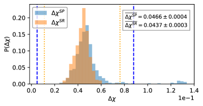
Here we present additional results in Fig. 5 for the statistics of and , similar to Fig. 2 in the main text at different shot counts . Dashed blue and dotted orange lines indicate the box-filtration fences according to the outlier filtering of Eq. 5 in the main text for and respectively. In all cases we identify a bump in at , for the nearest-neighbour complementary set of qubits only. As discussed in the main text, this bump corresponds to ‘bad qubits’ which leak considerable information (over 10% of a classical bit) into their surroundings. The fact that this bump is only visible in the nearest-neighbour complementary set data , and that it doesn’t change position with changing shot count, suggests that it is entirely independent of shot noise or other sources of error and is in fact a direct quantification of idle information loss.
We also note that, as the shout count is doubled between the panels Fig. 5(a)-(d), the centre of the main Gaussian distribution decreases; indicating that much of the signal is dominated by shot noise. We evaluate the mean values and their respective standard errors in the mean, both of which are shown in the inset boxes in each panel. The results of Welch’s t-tests identical to the one carried out in the main text are summarized in Table 1, indicating that the statistics for and are different to a high degree of statistical significance: with -values in excess of for all the results shown in Fig. 5. This indicates a positive detection of idle information loss at all shot counts investigated; even if the absolute value of this idle information loss is very small.
Finally, we note that at the higher shout counts and shown in Fig. 5(c) and Fig. 5(d) respectively, there is a finite probability of locating some results outside of the filter boundary but well below the threshold of for unambiguous ‘bad qubits’. This corresponds to qubits which are leaking enough information to be visible above the background of shot noise but which may not have failed completely.
Appendix B Details of State Tomography
State tomography in IBM devices is carried out by measuring all qubits in the output register , where indexes the physical location of the -th output qubit, simultaneously in the three Pauli bases. Taking the standard Pauli matrices, , , , , the statistics of each Pauli string with non-identity elements ( such that there are of this family of string in total) is determined by these measurements. The result of each measurement is a bitstring, and the result of a large number of measurements - called ‘shots’ - is a dictionary of bitstrings. Taking sufficiently large ensures that the sample statistics of measuring a specific bitstring given the Pauli string are close to the population statistics. These statistics for the reduced space of Pauli strings can then be aggregated into marginal values which yield statistics for the full space of Pauli strings. This is done by simply aggregating shots from different Pauli strings together wherever they coincide everywhere except where identities occur in the desired marginal.
| Shot Number | Complementary Set | Samples |
| 4000 | 609 | |
| 600 | ||
| 8000 | 507 | |
| 480 | ||
| 16000 | 324 | |
| 288 | ||
| 32000 | 252 | |
| 204 | ||
| 64000 | 157 | |
| 157 |
As a concrete example, consider an output register of three qubits, and lets say we are interested in the value of . This is given by the statistics of , , and . For each of these statistics, there is a corresponding dictionary of results where the are bitstrings which are simply the results of any single shot (measurement) given . The statistics of are given by calculation of the probability distribution . An example dictionary for for shots might be
| (7) |
with an associated probability distribution
| (8) |
Now consider the following example dictionaries for and :
| (9) | ||||
| (10) |
We then aggregate the dictionaries into a single new dictionary which describes the statistics of by simply excluding the central bit of each bitstring and aggregating the dictionaries:
| (11) | ||||
| (12) | ||||
| (13) | ||||
| (14) |
where contains 30 elements. The statistics of are then calculated as
| (15) |
We can now evaluate explicitly by summing up contributions to the expectation value , as follows
| (16) |
which completes our example.
This may seem a laborious process, but it allows us to extrapolate elements of a given state’s density matrix using only measurements. By decomposing the state’s density matrix into a sum of Pauli strings (including identity elements),
| (17) |
where is an appropriate normalization factor, we can readily reconstruct the quantum state of the output register using the dictionaries . These dictionaries are ultimately what IBM’s quantum computers return to their users. Where we discuss shot count in the main text, it simply refers the size of these returned dictionaries; where larger dictionaries more accurately yield the statistics of the actual population. The total number of samples of for both complementary qubit sets discussed in the main text (see Section II) is shown in Table 2 for all shot counts we consider.
Appendix C Aphysicality and Maximum-Likelihood Reconstruction
As discussed in Section III of the main text, shot noise due to finite can result in aphysical density matrices by introducing negative eigenvalues into their spectra. We correct for this using the maximum-likelihood reconstruction of the density matrix.
The tomographic process discussed in Appendix B yields a density matrix with matrix elements which is definitionally of trace unity and hermitian by inspection of Eq. 17. The eigenvalues of can, however, be negative; and thus is generally unphysical.
We follow and briefly summarize here the maximum-likelihood mixed state reconstruction algorithm given in the work of Smolin et al. [28]. First we invoke the existence of some density matrix with matrix elements and eigenvalues which minimizes the 2-norm,
| (18) |
where is the space of physical density matrices (unit trace, positive semi-definite, hermitian matrices). We remark here that Eq. 18 is invariant under change of basis, and hence we choose to work in the eigenbasis of with eigenvectors such that,
| (19) |
where is the Kronecker delta. Clearly, Eq. 19 is minimized when is also diagonal in this basis, i.e. the eigenvectors of are also , as any non-zero off-diagonal terms for strictly increases the value of Eq. 19. This reduces the minimization procedure down from an problem (where is the total dimension of the system) to a minimization problem in the eigenvalues of ,
| (20) |
subject to only two constraints: that , and that . The reconstructed density matrix is finally given by
| (21) |
For the system sizes that we consider, the minimization problem can be solved quickly by standard numerical minimization packages. This is the approach we use in the main text of this article. For larger problems, Smolin et al. provide a simple algorithm after reducing the complexity of the problem further by noting that the solution to Eq. 20 essentially involves finding a ‘pivot’ in the (ordered) wherein for and where is a constant for . The use of this algorithm is unnecessary for the situations we consider in this article, and we refer the interested reader to [28] for more details.