Nonparametric bootstrap of high-dimensional sample covariance matrices

Abstract

We introduce a new ”$(m,mp/n)$ out of $(n,p)$” sampling-with-replacement bootstrap for eigenvalue statistics of high-dimensional sample covariance matrices based on $n$ independent $p$-dimensional random vectors. In the high-dimensional scenario $p/n\rightarrow c\in(0,\infty)$, this fully nonparametric and computationally tractable bootstrap is shown to consistently reproduce the empirical spectral measure if $m/n\rightarrow 0$. If $m^{2}/n\rightarrow 0$, it approximates correctly the distribution of linear spectral statistics. The crucial component is a suitably defined Representative Subpopulation Condition which is shown to be verified in a large variety of situations. Our proofs are conducted under minimal moment requirements and incorporate delicate results on non-centered quadratic forms, combinatorial trace moments estimates as well as a conditional bootstrap martingale CLT which may be of independent interest.

SMReferences T1Supported by the DFG Research Unit 5381 Mathematical Statistics in the Information Age, project number 460867398, DE 502/30-1 and RO 3766/8-1

and

1 Introduction

Let $Y_{1},\dots,Y_{n}$ be independent, identically distributed $p$-dimensional centred random vectors with covariance matrix $\Sigma_{n}$ and corresponding sample covariance matrix

$$\widehat{\Sigma}_{n}=\frac{1}{n}\sum_{i=1}^{n}Y_{i}Y_{i}^{\top}.$$ (1.1)

We denote by $\hat{\lambda}_{1},\dots,\hat{\lambda}_{p}$ its eigenvalues, which are central objects in Principal Components Analysis (PCA). Classical text books (see, for example, Anderson,, 2003) provide asymptotic distributional results for the eigenvalues of the sample covariance matrix if the dimension $p$ is fixed and the sample size converges to infinity. These limit distributions are non-trivial, even in the Gaussian case, and depend in an intricate way on the unknown spectral distribution of population covariance matrix. In such situations bootstrap is an interesting alternative as it often has the ability to automatically address these difficulties by estimating unknown quantities by resampling. If the dimension is fixed and the sample size converges to infinity, the distribution of the eigenvalues of the sample covariance matrix can be consistently estimated by (nonparametric) bootstrap, where the resampling procedure has to be adapted, if there exist eigenvalues with multiplicity larger than one (see Beran and Srivastava,, 1985; Dümbgen,, 1993; Hall et al.,, 2009, among others).

On the other hand, in big data analysis the sample size $n$ and the dimension $p$ are often large and distributional approximations derived under the fixed $p$ scenario are usually not very accurate (see Johnstone,, 2006). In particular it is well known that if $p=p(n)$ increases proportionately with $n$, the eigenvalues of the sample covariance matrix are more dispersed than their population counterparts. The limiting spectral distribution (LSD) is described in terms of its Stieltjes transform as the solution of the Marc̆enko-Pastur (MP) equation, which relates the asymptotic behavior of the sample to the population eigenvalues. (Marčenko and Pastur,, 1967; Silverstein,, 1995). If $\min_{p,n\to\infty}p/n=c<1$ and $\Sigma_{n}=I_{p}$, where $I_{p}$ denotes the $p\times p$ identity matrix, the limiting spectral distribution can be determined explicitly and is supported on the interval$[(1-\sqrt{c})^{2},(1+\sqrt{c})^{2}]$. Similar results can be derived in the case $c\geq 1$, $\Sigma_{n}=I_{p}$. However, for a general population covariance matrix an explicit form, even for its support, is difficult to obtain because the MP equation is very hard to solve (see El Karoui,, 2008, for some work in this direction).

An intuitive solution to these problems seems to be the application of the bootstrap. However, results of El Karoui and Purdom, (2016, 2019) indicate that the classical bootstrap for the LSD is untrustworthy when the problem is genuinely high-dimensional. More precisely, in Theorem S2.2 in the supplementary material of their paper, El Karoui and Purdom, (2016) showed that the limiting spectral distribution (LSD) of the bootstrapped covariance matrix is completely different from that of $\widehat{\Sigma}_{n}$. To support these statements we show in the left part of Figure 1 the (simulated) density of the limit distribution of the empirical spectral measure of a sample covariance matrix and a histogram of the eigenvalues of the sample covariance matrix from a bootstrap sample drawn randomly with replacement. The dimension is $p=40000$, the sample size is $n=80000$ and the population covariance matrix is a diagonal matrix with $20000$ diagonal elements equal to $2$ and the remaining equal to $1$. One can clearly see that the “classical” $n$ out of $n$ bootstrap does not yield a reasonable approximation of the empirical spectral distribution.

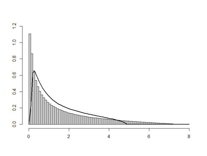
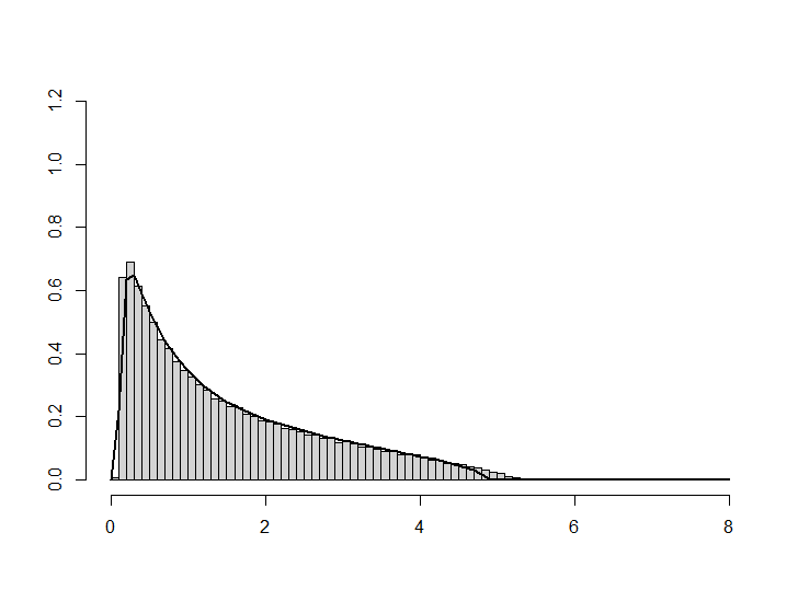
Figure 1: Left panel: histogram of the eigenvalues of an empircal covariance matrix from a bootstrap sample drawn randomly with replacement; Right panel: histogram of the eigenvalues of an empircal covariance matrix from the bootstrap sample drawn by the $(m,mp/n)$ out of $(n,p)$ proposed in this paper. Solid line (in both panels) the density of the limiting spectral distribution. The sample size is $n=80000$, the dimension $p=40000$ and the population covariance matrix is a diagonal matrix with $50\%$ of the entries equal to $1$ and $50\%$ equal to $2$.

Despite of these discouraging results, the aim of this article is to provide a powerful, fully nonparametric and computationally tractable tool to obtain accurate approximations for the distribution of the eigenvalues of the sample covariance matrix in the high-dimensional context. Our approach is based on the traditionally in a wider range applicable $m$ out of $n$ bootstrap (Politis and Romano,, 1994; Bickel et al.,, 1997), which has already been investigated to approximate the eigenvalue distribution in the case where the dimension is fixed. However, the use of this approach in the high-dimensional setting presents another challenge as it does not even preserve the limiting ratio $c$ of dimension and sample size if $m\ll n$, which appears already explicitly in the characterizing Marc̆enko-Pastur equation for the Stieltjes transform of the LSD (see Marčenko and Pastur,, 1967; Silverstein,, 1995). To address this difficulty, we propose to also select (possibly by a random mechanism) $q=\lfloor mp/n\rfloor$ coordinates from the estimator for the covariance matrix obtained from the subsample of $m$ observations such that the ratio of dimension and sample size remains (asymptotically) unchanged. This procedure will be called “$(m,mp/n)$ out of $(n,p)$ bootstrap” throughout this paper and is based on the crucial observation that in many situations of interest, a subvector of $Y_{1}$, selected according to an appropriate random sampling mechanism, provides a covariance matrix, say $\tilde{\Sigma}_{n}$, with a similar spectral distribution as the covariance matrix $\Sigma_{n}$ of the full vector $Y_{1}$. We will prove that under the so-called Representative Subpopulation Condition and minimal moment requirements, the ”$(m,mp/n)$ out of $(n,p)$” bootstrap provides a consistent approximation of the Marc̆enko-Pastur distribution if $m=o(n)$. Moreover, it consistently mimics the distribution of linear spectral statistics (LSS’) of the sample covariance matrix if $m=o(\sqrt{n})$. Appealingly, the simultaneously reduced dimension and sample size make its implementation computationally tractable even if original dimension and sample size are very large. In the right panel of Figure 1 we show the histogram of the empirical spectral distribution where the sample is obtained by ”$(m,mp/n)$ out of $(n,p)$” bootstrap with subsample size $m=8000$, and where the $p$-dimensional data is projected on $q=mp/n=4000$ randomly chosen coordinates. We observe a reasonable approximation of the limiting distribution.

We conclude this section with a discussion of related work on bootstrap for the spectrum of high-dimensional covariance matrices. El Karoui and Purdom, (2016, 2019) investigated the nonparametric bootstrap and demonstrated that this method is in general not a reliable tool for statistical inference in the high-dimensional regime. They also argued that for the largest eigenvalues the nonparametric bootstrap performs as it does in finite dimension if the population covariance matrix can be well approximated by a finite rank matrix. Han et al., (2018) proposed a multiplier bootstrap based on a high-dimensional Gaussian approximation to approximate the distribution of the largest eigenvalue of the sample covariance matrix under the assumption of a spherical population covariance matrix. However, the validity of this procedure can only be proved under very restricted assumptions on the increasing dimension, that is $p=o(n^{1/9})$. Yao and Lopes, (2022) derived finite sample bounds for the Kolmogorov distance between the distribution of the largest eigenvalue and a bootstrap distribution obtained by sampling with replacement in terms of the effective rank of the population covariance matrix and sample size. More recently, Ding et al., (2023) investigated the extreme eigenvalues of the sample covariance matrix under the generalized elliptical model. As a special case they considered a factor model and developed a multiplier bootstrap test for the number of factors by investigating the stochastic properties of the first few eigenvalues of the bootstrap sample covariance matrix (see also Yu et al.,, 2024, who directly concentrate on a high-dimensional factor model).
While most of this work has its focus on the extreme eigenvalues, the bootstrap for linear spectral statistics of high-dimensional covariance matrices is much less explored. Lopes et al., (2019) proposed a parametric type bootstrap method in the high-dimensional setting sampling bootstrap data from a proxy distribution that is parameterized by estimates of the eigenvalues and kurtosis. Roughly speaking these authors suggested to generate a matrix of the form (1.1) from independent random vectors with iid. Pearson distributed entries (matching the first four moments asymptotically) and to multiply the resulting matrix from the left and the right by a square root of the diagonal matrix containing the spectrum. We also mention the paper of Wang and Lopes, (2023) who developed a parametric type bootstrap for linear spectral statistics in the high-dimensional elliptical model, which uses the specific structure of this model and also requires the estimation of a diagonal matrix containing the spectrum. In contrast to these authors the bootstrap procedure proposed here is completely nonparametric, does not require estimation of the spectrum of the population covariance matrix and is provably consistent under minimal moment assumptions. As a consequence we do not need assumptions on the limiting spectrum of the population covariance matrix which are usually required to make its estimation possible.

2 Preliminaries

For any Hermitian matrix $A\in\mathbb{C}^{p\times p}$ with eigenvalues $\lambda_{1}(A),\dots,\lambda_{p}(A)$,

$$\mu^{A}=\frac{1}{p}\sum_{i=1}^{p}\delta_{\lambda_{i}(A)}$$

denotes its (normalized) spectral measure. For any matrix $A$, we write $A^{\top}$ for its transpose of $A$ and $\bar{A}$ for its complex conjugate. For $1\leq r\leq\infty$, we denote by $\|A\|_{S_{r}}=\big{(}\sum_{j=1}^{p}\lambda_{j}(A\bar{A}^{\top})^{r/2}\big{)}^{1/r}$ the Schatten-$r$-norm of the matrix $A$. The Stieltjes transform of a distribution $G$ on the real line is given by $m_{G}:\mathbb{C}^{+}\rightarrow\mathbb{C}^{+}$ with

$$m_{G}(z)=\int{1\over\lambda-z}dG(\lambda),$$

where $\mathbb{C}^{+}=\{z\in\mathbb{C}\arrowvert\,\Im(z)>0\}$ denotes the upper complex half-plane. If $\mu_{n}$, $n\in\mathbb{N}$, and $\mu$ are finite signed measures on a common measurable space, $\mu_{n}\Rightarrow\mu$ denotes weak convergence of $(\mu_{n})_{n\in\mathbb{N}}$ to $\mu$.

Model assumptions. Aligning with the common framework in random matrix theory, we shall work under the same type of conditions and study a triangular array of $p=p(n)$-dimensional observations $Y_{1},\dots,Y_{n}$ of the form

$$Y_{i}=A_{n}X_{i},\ \ \ i=1,\dots,n.$$ (2.1)

Here, $X_{i}=(X_{i1},X_{i2},\ldots)^{\top}$ $(i\in\mathbb{N})$ are independent identically distributed (iid) infinite dimensional random vectors and $A_{n}$ is a $p\times\infty$ matrix such that the following assumptions are satisfied:

• The $(p\times\infty)$-matrix $A_{n}$ has square summable rows and $\sup_{n\in\mathbb{N}}\|A_{n}\|_{S_{\infty}}<\infty$.

• $p/n\rightarrow c$ for some real constant $c>0$ as $n\rightarrow\infty$.

• The vector $X_{1}$ has iid entries $X_{1k}$, $k\in\mathbb{N}$, with $\mathbb{E}X_{11}=0$ and $\mathbb{E}X_{11}^{2}=1$.

Note that under these conditions, the random variable $Y_{1}=A_{n}X_{1}$ is well defined as limit in $L^{2}(\mathbb{P})$ with covariance matrix

$$\Sigma_{n}=\mathbb{E}[Y_{1}Y_{1}^{\top}]=A_{n}A_{n}^{\top}~{}.$$

As concerns normal approximation of linear spectral statistics, the existence of the fourth moment $\mathbb{E}X_{11}^{4}<\infty$ is known to be necessary. Therefore, we shall impose in that case the stronger assumption

• In addition to assumption (A3), $\mathbb{E}X_{11}^{3}=0$ and $\mathbb{E}X_{11}^{4}=3$.

Coincidence of the third and fourth moment with those of the standard normal distribution can be avoided in the CLT for linear spectral statistics of high-dimensional covariance matrices at the expense of additional regularity assumptions on the eigenvectors, see Najim and Yao, (2016). Here, we refrain from this generalization to keep the technical expenditure as small as possible. We emphasize that model (2.1) was also considered in Zou et al., (2022) and contains the commonly used model

$$Y_{i}=\Sigma_{n}^{1/2}\tilde{X}_{i},$$ (2.2)

where $\tilde{X}_{i}$ is a $p$-dimensional with iid entries $\tilde{X}_{ik}$ ($\mathbb{E}\tilde{X}_{11}=0$, $\mathbb{E}\tilde{X}_{11}^{2}=1$) and $\Sigma_{n}^{1/2}$ is the square root of the $p\times p$ matrix $\Sigma_{n}$. For model (2.2), it is well-known that if $(\mu^{\Sigma_{n}})$ is weakly convergent as $p,n\to\infty$ and $p/n\to c\in(0,\infty)$, that is

$$\mu^{\Sigma_{n}}\Rightarrow H\ \ \text{as}\ n\rightarrow\infty$$ (2.3)

for some distribution $H$, the limiting spectral distribution (LSD) of the sample covariance matrix exists and is given by the Marc̆enko-Pastur law $\mu_{H}^{0}$ whose Stieltjes transform can be characterized as the unique solution of the Marc̆enko-Pastur (MP) equation

$$m_{H}^{0}(z)=\int\frac{1}{\lambda(1-c-czm_{H}^{0}(z))-z}dH(\lambda).$$ (2.4)

These results were extended to model (2.1) by Zou et al., (2022). Finally, we define for a distribution $G$ on the real line $\underline{m}_{G}^{0}$ as the unique solution in $\mathbb{C}^{+}$ of the equation

$$\underline{m}_{G}^{0}(z)=-\bigg{(}z-c\int\frac{t}{1+t\underline{m}_{G}^{0}(z)}\operatorname{d}G(t)\bigg{)}^{-1}.$$ (2.5)

Note that

$$\underline{m}_{G}^{0}(z)=-\frac{1-c}{z}+cm_{G}^{0}(z),$$

where $m_{G}^{0}(z)$ is the solution of the equation (2.4) for $H=G$.

3 Representative subpopulations and the ”$(m,mp/n)$ out of $(n,p)$” bootstrap

The $m$ out of $n$ sampling-with-replacement bootstrap with $m=o(n)$ provides a powerful methodology for constructing valid bootstrap procedures in situations where the classical bootstrap “resampling with replacement” does not work (Politis and Romano,, 1994; Bickel et al.,, 1997). However, in the high dimensional regime $p/n\to c>0$ as $n\to\infty$ the properties of the LSD and LSS’ depend sensitively of the “proportion” $c$ and the application of this methodology is not obvious as a sample covariance matrix based on a random sample of $m$ observations from $Y_{1},\ldots,Y_{n}$ with $m=o(n)$ would exhibit an asymptotic behaviour as in the case $c=\infty$. To address this difficulty, we propose to also sample (possibly by a randomly mechanism) $q=\lfloor mp/n\rfloor$ coordinates from the estimator of the covariance matrix obtained from the subsample of $m$ observations such that $q/m\to c$ as $n\to\infty$, $m\to\infty$, $m=o(n)$. Interpreting the entries $Y_{i1},\dots,Y_{i_{p}}$ of each vector $Y_{i}$ as data of $p$ individuals in some population, our approach originates from the idea of selecting a representative subpopulation which shares the statistical properties of interest with the full population.

This procedure will be called “$(m,mp/n)$ out of $(n,p)$ bootstrap” throughout this paper and is based on the crucial observation that in many situations of interest, a subvector $Y_{1,sub}$ of length $q=q(n)$ of $Y_{1}$, selected according to an appropriate (random) sampling mechanism, provides a $q\times q$ covariance matrix, say $\tilde{\Sigma}_{n}$, with a similar spectral distribution, say $\mu^{\tilde{\Sigma}_{n}}$, as the spectral distribution $\mu^{\Sigma_{n}}$ of the population covariance matrix $\Sigma_{n}$ corresponding to the full vector $Y_{1}$, that is

$$\mu^{\tilde{\Sigma}_{n}}-\mu^{\Sigma_{n}}\Rightarrow 0\ \ \text{as}\ n\rightarrow\infty\ \ \text{in probability}.$$ (3.1)

To illustrate this observation we present three examples.

Example 3.1 (Diagonal positive semi-definite matrices).

Let

$$(\Sigma_{n})_{n\in\mathbb{N}}=(\text{diag}(g_{1},\ldots,g_{p}))_{n\in\mathbb{N}}$$

denote a sequence of positive semi-definite diagonal matrices satisfying (2.3), that is

$$\frac{1}{p}\sum^{p}_{i=1}\delta_{g_{i}}\Longrightarrow H$$ (3.2)

for some distribution function $H$. If $Y_{1,sub}$ consists of $q$ out of $p$ different entries of the vector $Y_{1}$ uniformly sampled at random, its covariance matrix, say $\tilde{\Sigma}_{n},$ is a principal $q\times q$ submatrix sampled uniformly at random from $\Sigma_{n}$. Hence, by Theorem 1 of Chatterjee and Ledoux, (2009) and assumption (2.3) it follows that (3.1) holds.

More generally, let $M$ be an arbitrary Hermitian matrix of order $n$ and $k$ be a positive integer less than $n$. Chatterjee and Ledoux, (2009) prove the remarkable result that if $k$ is large, the distribution of eigenvalues on the real line is almost the same for almost all principal submatrices of $M$ of order $k$.

Example 3.2 (Symmetric Toeplitz and block Toeplitz matrices).

• If the components of the vectors $Y_{i}=(Y_{i,\ell})_{\ell=1,\ldots p}$ are defined by a stationary process, then it follows by Wold’s theorem (see Brockwell and Davis,, 1998) that

  $$Y_{i,\ell}=\sum^{\infty}_{j=0}b_{j}X_{i,p-\ell+j+1}$$ (3.3)

  where $\sum_{j=0}^{\infty}b_{j}^{2}<\infty$ and for each $i$ the random variables in the vector $X_{i}=(X_{i,j})_{j\in\mathbb{N}}$ are uncorrelated. If the random variables $X_{i,j}$ are independent with $\mathbb{E}X_{11}=0$, $\mathbb{E}X_{11}^{2}=1$ (as assumed in the present paper) we obtain a representation of the form (2.1), where the $p\times\infty$ matrix $A_{n}$ is given by

  $$A_{n} = \left(\begin{array}[]{ccccccccc}0&0&\ldots&\ldots&{\ldots}&0&b_{0}&b_{1}&{\ldots}\\ 0&0&\ldots&\ldots&{\ldots}&b_{0}&b_{1}&b_{2}&{\ldots}\\ \vdots&\vdots&\ddots&\ddots&\ddots&\ddots&\ddots&\ddots&{\cdots}\\ 0&0&b_{0}&b_{1}&\cdots&b_{p-4}&b_{p-3}&b_{p-2}&\cdots\\ 0&b_{0}&b_{1}&b_{2}&\cdots&b_{p-3}&b_{p-2}&b_{p-1}&\cdots\\ b_{0}&b_{1}&b_{2}&b_{3}&\cdots&b_{p-2}&b_{p-1}&b_{p}&{\ldots}\end{array}\right).$$ (3.10)

  Note that the $p\times p$ autocovariance matrix

  $$\Sigma_{n}=A_{n}A^{\top}_{n}=(t_{i-j})^{p}_{ij=1}$$

  is a Toeplitz matrix, where

  $$t_{k}={\rm Cov}(Y_{i,\ell},Y_{i,\ell-k})=\sum^{\infty}_{j=k}b_{j}b_{j-k}=\sum^{\infty}_{j=0}b_{j}b_{j+k}$$

  (note that $t_{-\ell}=t_{\ell}$). In particular $\Sigma_{n}$ is a $p\times p$ principal minor of the fixed (infinite) Toeplitz matrix $(t_{i-j})_{ij\in\mathbb{N}}$. Now, if $\sum^{\infty}_{\ell=0}|t_{\ell}|<\infty$, it follows from Szegö’s theorem (see Grenander and Szego,, 1958) that the normalized spectral distribution of $\Sigma_{n}$ satisfies (2.3), where the limiting distribution $H$ is supported on the interval $(-\pi,\pi]$. More precisely, $\mu^{\Sigma_{n}}\Rightarrow H$ as $n\to\infty$, where the measure $H$ is defined by

  $$H((-\alpha,\beta])=\frac{1}{2\pi}\lambda\big{(}\big{\{}t\in(-\pi,\pi]\big{|}\alpha<T(e^{it})\leq\beta\big{\}}\big{)}$$

  and $T(z)$ is the Laurent series

  $$T(z)=t_{0}+2\sum^{\infty}_{\ell=1}t_{\ell}(z^{\ell}+z^{-\ell}).$$

  If $\tilde{\Sigma}_{n}$ is a $q\times q$ principal minor of $\Sigma_{n}$, then obviously its spectral distribution converges weakly to $H$ as $q\to\infty$. Consequently, if $Y_{1,sub}$ consists of $q$ consecutive entries of $Y_{1}$, its covariance matrix is equal to $\Sigma_{q}$, and spectral similarity holds in the sense of (3.1).

  Note that in this example, it is not even necessary to rely on a random sampling mechanism.

• If $p=\tilde{p}r$ for some $\tilde{p},r\in\mathbb{N}$, similar results are available in the case where the components of the vectors $Y_{i}$ can be decomposed in $\tilde{p}$ block of length $r$, that is

  $$Y_{i}=\big{(}Y^{(1)\top}_{i},\ldots,Y^{(\tilde{p})\top}_{i}\big{)}^{\top}\qquad i=1,\ldots,n,$$

  which are defined by a vector moving average model of order $\ell\leq\tilde{p}-1$, that is

  $$Y^{(s)}_{i}=\sum^{\ell}_{j=0}B_{j}\varepsilon_{i,\tilde{p}-s+j+1}~{},~{}~{}s=1,\ldots,\tilde{p}.$$

  Here ($\varepsilon_{i,j})_{i\in\mathbb{N},j\in\mathbb{N}_{0}}$ is an array of independent $r$-dimensional vectors with $\mathbb{E}[\varepsilon_{ij}]=0\in\mathbb{R}^{r}$ and Var$(\varepsilon_{ij})=I_{r}$, $I_{r}$ denotes the $r$-dimensional identity matrix and $B_{0},\ldots,B_{k}$ are given $r\times r$ matrices. In this case, it is easy to see that the population covariance matrix $\Sigma_{n}$ of $Y_{i}$ is a banded block Toeplitz matrix, that is

  $$\Sigma_{n}=\big{(}T_{|i-j|}I\{|i-j|\leq\ell\}\big{)}^{\tilde{p}}_{i,j=1}~{},$$ (3.11)

  where $T_{0},\ldots,T_{\ell}$ are symmetric $r\times r$ matrices defined by

  $$T_{s}=\sum_{j=0}^{\ell-s}B_{j}B_{j+\ell}^{\top}~{},~{}~{}s=0,\ldots\ell-1$$

  (and $T_{\ell+1}=\ldots=T_{\tilde{p}-1}=I_{r}$). If $\tilde{p}\to\infty$, the LSP of the population covariance matrix exists and can be characterized in terms of an equilibrium problem (see Delvaux,, 2012). However, an explicit form is only possible in very special cases. For example, if $\ell=1$, $T_{1}$ is a a non-singular matrix, such that $\lim_{n\to\infty}T^{-n}_{1}T_{0}T_{1}^{n}=T_{\rm lim}$ exists, the LSD is absolute continuous with respect to the Lebesgue measure with density

  $$f(t)=\frac{1}{r}\mbox{tr}\big{(}X_{T_{1},T_{\rm lim}}(t)\big{)}$$

  where $X_{T_{1},T_{\rm lim}}$ is the density of the matrix measure of orthogonality corresponding to matrix Chebyshev polynomials of the first kind with recurrence coefficients ${T_{1},T_{\rm lim}}\in\mathbb{R}^{r\times r}$ (see, for example, Duran et al.,, 1999). Now, if $\tilde{\Sigma}_{n}$ is a $q\times q$ principal minor of $\Sigma_{n}$ maintaining the block structure of $\Sigma_{n}$, then (3.1) obviously holds.

Example 3.3 (Representative subpopulations).

In a recent paper Fan and Johnstone, (2019) investigated properties of the LSP of variance components in linear random effect models. In the simplest case of a random effect ANOVA model with $k$ factors, we have

$$\tilde{Y}_{ij}=M_{i}+s_{ii}X_{ij}\qquad\qquad j=1,\ldots,p_{i}\ ;\quad i=1,\ldots,k,$$ (3.12)

$s_{11},\ldots,s_{kk}>0$ are constants, $\{X_{ij}|~{}j=1,\ldots,p_{i};i=1,\ldots,k\}$ are independent random variables with $\mathbb{E}[X_{ij}]=0$, ${\rm Var}(X_{ij})=1$ and $M=(M_{1},\ldots,M_{k})^{\top}$ is a $k$-dimensional random vector with covariance matrix $T=(\tau_{ij})^{k}_{i,j=1}$ representing the group effects. In this case the vector $Y_{1}$ can be decomposed in $k$ groups, that is

$$Y^{\top}_{1}=(\tilde{Y}_{11},\ldots,\tilde{Y}_{1p_{1}},\tilde{Y}_{21},\ldots,\tilde{Y}_{2p_{2}},\ldots,\tilde{Y}_{k_{1}},\ldots,\tilde{Y}_{kp_{k}})^{\top}\in\mathbb{R}^{p}~{},$$

where $p=\sum_{i=1}^{k}p_{i}$. With the notation $s_{ii}=\sqrt{\sigma_{ii}-\tau_{ii}}$ with $\sigma_{ii}=s^{2}_{ii}+\tau_{ii}$ $(i=1,\ldots,k)$ the covariance matrix of the vector $Y_{1}$ is given by the positive semi-definite symmetric block matrix

$$\Sigma_{n}=\left(\begin{matrix}G_{11}&G_{12}&G_{13}&\dots&G_{1k}\\ G_{21}&G_{22}&G_{23}&\dots&G_{2k}\\ \vdots&\vdots&\vdots&\ddots&\vdots\\ G_{k1}&G_{k2}&G_{k3}&\dots&G_{kk}\end{matrix}\right)$$

with blocks

$$G_{ii}=\left(\begin{matrix}\sigma_{ii}&\tau_{ii}&\dots&\tau_{ii}\\ \tau_{ii}&\sigma_{ii}&\dots&\tau_{ii}\\ \vdots&\vdots&\ddots&\vdots\\ \tau_{ii}&\tau_{ii}&\dots&\sigma_{ii}\end{matrix}\right)\in\mathbb{R}^{p_{i}\times p_{i}},~{}G_{ij}=\tau_{ij}\left(\begin{matrix}1&1&\dots&1\\ 1&1&\dots&1\\ \vdots&\vdots&\ddots&\vdots\\ 1&1&\dots&1\\ \end{matrix}\right)\in\mathbb{R}^{p_{i}\times p_{j}}~{}(i\not=j).$$

A simple calculation shows that the matrix $\Sigma_{n}$ has at most $2k$ different eigenvalues and that there are $k$ eigenvalues $\lambda_{i}=\sigma_{ii}-\tau_{ii}$ of multiplicity $p_{i}-1$ ($i=1,\ldots,k$). Therefore, if $k=o(p)$ and there exist nonnegative constants $\omega_{1},\ldots\omega_{k}$ such that $\sum_{i=1}^{k}\omega_{i}=1$ and $\max^{k}_{i=1}|\frac{p_{i}}{p}-\omega_{i}|=o(1)$ as $n\to\infty$, $p_{i}\to\infty$, the sequence $(\mu^{\Sigma_{n}})_{n\in\mathbb{N}}$ of spectral measures converges weakly to the discrete measure $\sum^{k}_{i=1}\omega_{i}\delta_{\lambda_{i}}$. If $Y_{1,sub}$ consists of $q$ out of $p$ different entries of the vector $Y_{1}$ uniformly sampled at random without replacement, its covariance matrix ${\tilde{\Sigma}_{n}}$ has again at most $2k$ different eigenvalues and there exist $k$ eigenvalues $\lambda_{i}=\sigma_{ii}-\tau_{ii}$ of multiplicity $\max(q_{i}-1,0)$ ($i=1,\ldots,k$), where $(q_{1},\ldots,q_{k})$ is amultivariate hypergeometrically distributed random variable with parameters $((p_{1},\ldots,p_{k}),q)$. Consequently, condition (3.1) is satisfied.

Motivated by these examples we introduce the following condition, which will be crucial in the analysis of the “$(m,mp/n)$ out of $(n,p)$ bootstrap” introduced afterwards.

Condition 3.4 (Representative Subpopulation Condition).

The triangular array of $p$-dimensional vectors $Y_{1},\dots,Y_{n}$ in model (2.1) is said to satisfy the Representative Subpopulation Condition, if the following conditions are satisfied.

• For every $q\leq p$, there exists a possibly random strategy (independent of $Y_{1},\dots,Y_{n}$) of selecting q out of $p$ coordinates such that the covariance matrix ${\tilde{\Sigma}_{n}}$ of the resulting $q$-dimensional subvectors $Y_{i,sub}$ ($i=1,\dots,n$) satisfies

  $$\mu^{\tilde{\Sigma}_{n}}-\mu^{\Sigma_{n}}\Rightarrow 0\ \ \text{as}\ q,n\rightarrow\infty\ \ \text{in probability}.$$ (3.13)

• If $\Pi_{n}=\Pi_{n,q}$ denotes the projection corresponding to the possibly random selection strategy, that is $Y_{i,sub}=\Pi_{n}Y_{i}$ ($i=1,\dots,n$), then there exists for almost all realizations a decomposition of the form

  $$\Pi_{n}A_{n}=L_{n}+R_{n}~{},$$ (3.14)

  where the sets of non-zero entries of the matrices $L_{n}$ and $R_{n}$ are disjoint, the matrix $L_{n}$ has a most $q^{\prime}$ non-zero columns with $q^{\prime}$ a possibly random integer of deterministic order $O(q)$, and $\mathbb{E}_{\Pi_{n}}\big{[}||R_{n}||_{S_{2}}^{2}\big{]}=o(1)$ as $q,n\rightarrow\infty$. Here, $\mathbb{E}_{\Pi_{n}}$ denotes expectation with respect to the random projection $\Pi_{n}$.

Remark 3.5.

(a) Note that (3.13) refers to the population covariance matrix $\Sigma_{n}$ and that randomness enters in the submatrix $\tilde{\Sigma}_{n}$ of $\Sigma_{n}$ only through the random coordinate selection. Interpreting the $p=p(n)$ entries of $Y_{1}$ as the individuals of a population with their $p\times p$ covariance matrix $\Sigma_{n}$, the weak convergence assumption (3.13) is justified by the belief that the spectral measure encodes information of the population, and that a representative subpopulation behaves qualitatively in the same way as the full population.
(b) Note that Assumption (A1) implies in particular that the spectral norm of the matrix $\tilde{\Sigma}_{n}=\Pi_{n}\Sigma_{n}\Pi_{n}$ is uniformly bounded in $n\in\mathbb{N}$.

The Representative Subpopulation Condition being granted, we propose the following resampling scheme.

Algorithm 3.6 ( $(m,mp/n)$ out of $(n,p)$ Bootstrap).

• For $m=o(n)$, draw an iid sample $Y_{1}^{*},\dots,Y_{m}^{*}$ from the empirical distribution

  $$\hat{\mathbb{P}}_{n}=\frac{1}{n}\sum_{i=1}^{n}\delta_{Y_{i}}.$$

• Define the bootstrap sample

  $$Z_{i}^{*}=\Pi_{n}Y^{*}_{i}=(Y_{ij_{1}}^{*},\dots,Y_{ij_{q}}^{*})^{\top},\ \ i=1,\dots,m,$$

  using the $q=\lfloor mp/n\rfloor$ coordinates $j_{1},\dots,j_{q}$ selected according to the Representative Subpopulation Condition.

• Output: the estimator

  $$\hat{\Sigma}_{n}^{*}={1\over m}\sum_{i=1}^{m}Z_{i}^{*}{Z_{i}^{*}}^{\top}=\Pi_{n}\Big{(}{1\over m}\sum_{i=1}^{m}Y^{*}_{i}{Y^{*}_{i}}^{\top}\Big{)}\Pi_{n}^{\top}$$

  and its corresponding spectral distribution $\mu^{\hat{\Sigma}_{n}^{*}}$.

In the following section we will show that under appropriate assumptions, Algorithm 3.6 yields a consistent bootstrap estimate of the LSD and of the distribution of linear spectral statistics. We conclude this section revisiting Examples 3.1 – 3.3, where the Representative Subpopulation Condition is satisfied and – as a consequence of the theory developed in the subsequent Section 4 – the $(m,mp/n)$ out of $(n,p)$ bootstrap is consistent.

Example 3.7.

In the situation of Example 3.1 we assumed that the empirical distribution function of the points $g_{1},\ldots,g_{p}$ converges weakly, to some distribution function $H$ (see (3.2)). In this case, the matrix $A_{n}$ in (2.1) is given by $A_{n}={\rm diag}(g_{1},\ldots,g_{p},0,0\ldots)$. If $Y^{*}_{1},\ldots,Y^{*}_{m}$ are sampled uniformly at random from $Y_{1},\ldots,Y_{n}$, then it is easy to see that $\mu^{\tilde{\Sigma}_{n}}\Longrightarrow H$ in probability and (3.13) is satisfied. Moreover, (3.14) also holds using $L_{n}=\Pi_{n}{\rm diag}(g_{1},\ldots,g_{p})\in\mathbb{R}^{q\times p},R_{n}=0\in\mathbb{R}^{q\times\infty}$ and $\Pi_{n}\in\mathbb{R}^{q\times p}$ corresponds to the random projection which picks $q$ coordinates from $(1,\ldots,p)$ uniformly at random without replacement.

Example 3.8.

Recall the model considered in Example 3.2 and let $\Pi_{n}$ denote the projection which selects the first $q$ components of the vector $Y_{1}$ defined in (3.3). Then, recalling the definition of the matrix $A_{n}$ in (3.10), a decomposition of the form (3.14) holds with

$$~{}~{}~{}~{}~{}L_{n} = \left(\begin{array}[]{ccccccccccc}0&0&0&\cdots&0&b_{0}&\cdots&b_{q}&0&0&\cdots\\ 0&0&0&\cdots&b_{0}&b_{1}&\cdots&b_{q+1}&0&0&\cdots\\ \vdots&\vdots&\vdots&\ddots&\vdots&\vdots&\ddots&\vdots&\vdots&\vdots&\ddots\\ 0&0&b_{0}&\cdots&b_{q-4}&b_{q-3}&\cdots&b_{2q-3}&0&0&\cdots\\ 0&b_{0}&b_{1}&\cdots&b_{q-3}&b_{q-2}&\cdots&b_{2q-2}&0&0&\cdots\\ b_{0}&b_{1}&b_{2}&\cdots&b_{q-2}&b_{q-1}&\cdots&b_{2q-1}&0&0&\cdots\end{array}\right)~{}$$

and

$$R_{n} = \left(\begin{array}[]{ccccccc}0&0&\cdots&0&b_{q+1}&b_{q+2}&\cdots\\ 0&0&\cdots&0&b_{q+2}&b_{q+3}&\cdots\\ \vdots&\vdots&\ddots&\vdots&\vdots&\vdots&\ddots\\ 0&0&\cdots&0&b_{2q-2}&b_{2q-1}&\cdots\\ 0&0&\cdots&0&b_{2q-1}&b_{2q}&\cdots\\ 0&0&\cdots&0&b_{2q}&b_{2q+1}&\cdots\end{array}\right)~{}$$

(note that both matrices have $q$ rows and that the first $2q$ columns of the matrix $R_{n}$ have zero entries). Now under the additional assumption that

$$\sum^{\infty}_{\ell=1}\ell b^{2}_{\ell}<\infty,$$

it is easy to see that

$$\|L_{n}\|^{2}_{S_{2}} = q\sum^{q}_{i=0}b^{2}_{i}+\sum^{2q-1}_{i=q+1}(2q-i)b^{2}_{i}=O(q)$$

$$\|R_{n}\|^{2}_{S_{2}} = \sum^{q}_{i=1}\sum^{\infty}_{\ell=i}b^{2}_{q+\ell}\leq q\sum^{\infty}_{\ell=q+1}b^{2}_{\ell}\leq\sum^{\infty}_{\ell=q+1}\ell b^{2}_{\ell}=o(1)$$

as $n\to\infty$. A similar argument applies if $q$ consecutive components of $Y_{1}$ are sampled from a uniformly distributed position on the set $\{1,\ldots,p-q+1\}$. Hence, the triangular array $(Y_{1},\dots,Y_{n})$ satisfies the Representative Subpopulation Condition (note that the first assumption in Condition 3.4 was shown in Example 3.2).

Example 3.9.

Note note that model (3.12) in Example 3.3 can be rewritten as

$$Y_{1}=EM+SX~{},$$ (3.17)

where

$$X = \big{(}X_{11},\ldots,X_{1p_{1}},\ldots,X_{k1},\ldots,X_{kp_{k}})^{\top}\in\mathbb{R}^{p},$$

$$M = \big{(}M_{1},\ldots,M_{k})^{\top}\in\mathbb{R}^{k},$$

the $p\times k$ matrix $E$ and the $p\times p$ matrix $S$ are defined by

$$E = \left(\begin{array}[]{cccc}1_{p_{1}}&&&\\ &1_{p_{2}}&&\\ &&\ddots\\ &&&1_{p_{k}}\end{array}\right)\in\mathbb{R}^{p\times k}~{},~{}~{}S=\left(\begin{array}[]{cccc}s_{11}I_{p_{1}}&&&\\ &s_{22}I_{p_{2}}&&\\ &&\ddots\\ &&&s_{kk}I_{p_{k}}\end{array}\right)\in\mathbb{R}^{p\times p}~{},$$

respectively, and $1_{p_{\ell}}=(1,\ldots,1)^{\top}\in\mathbb{R}^{p_{\ell}}$ (all other entries in the matrices $E$ and $S$ are $0$). The model (3.17) can alternatively be represented (in distribution) as

$$Y_{1}=\tilde{E}Z$$ (3.19)

where $Z=(X^{\top},U^{\top})^{\top}\in\mathbb{R}^{p+k},U=(U_{1},\ldots,U_{k})^{\top}$ is a vector with iid entries independent of $X$, such that $\mathbb{E}[U_{i}]=0$, ${\rm Var}(U_{i})=1$ and the $p\times(p+k)$ matrix $\tilde{E}$ is given by

$$\tilde{E}=(S:ET^{1/2})~{}.$$

The model (3.19) can obviously written in the form (2.1). Moreover, the matrix $L_{n}$ in the decomposition (3.14) is given by $q$ randomly drawn rows from the matrix $\tilde{E}$, while the matrix $R_{n}$ has only $0$ entries. As the matrix $S$ is diagonal, the matrix $L_{n}$ has at most $q+k=O(q)$ non-zero columns, and the triangular array in Example 3.3 satisfies the Representative Subpopulation Condition.

4 Probabilistic properties of the ’$(m,mp/n)$ out of $(n,p)$’ bootstrap

In view of the failure of the classical sampling-with-replacement bootstrap, it is apparent that independence of the bootstrap observations $(Z_{1}^{*},\ldots,Z_{m}^{*})=(\Pi_{n}A_{n}X_{1}^{*},\ldots,\Pi_{n}A_{n}X_{m}^{*})$ conditionally on the original data $Y_{1},\ldots,Y_{n}$ and $\Pi_{n}$ cannot be sufficient to successfully run classical arguments in the conditional bootstrap world for proving consistency of our new approach. Indeed, the vectors $X_{i}^{*}$ do not satisfy Assumption (A3) any longer (conditional on $X_{1},\dots,X_{n}$); in particular, they do not possess the essential structure of independent components which however is a crucial requirement for the classical MP law and the CLT of linear spectral statistics to hold.

4.1 Spectral distribution

Our first result demonstrates that $\widehat{\Sigma}_{n}^{*}$ mimics the sample covariance matrix in terms of spectral distributions. Besides being of interest in its own, this is a necessary ingredient for the CLT for linear spectral statistics studied later as the limiting spectral distribution of the sample covariance matrix explicitly enters the limiting variance expression of linear spectral statistics.

Theorem 4.1 (Spectral distribution).

Grant assumptions (A1)–(A3). Suppose that the triangular array of $p$-dimensional vectors $Y_{1},\dots,Y_{n}$ in model (2.1) satisfies the Representative Subpopulation Condition 3.4. If $m=o(n)$, then

$$\mu^{\widehat{\Sigma}_{n}}-\mu^{\widehat{\Sigma}_{n}^{*}}\Longrightarrow 0~{}~{}\text{ in probability. }$$

As concerns the proof of Theorem 4.1, note that the derivation of the classical MP-law via the Stieltjes transform method has two major steps:

• to establish the concentration of the Stieltjes transform of the bootstrap spectral measure around its conditional expectation (see equation (B.30) in the online supplement);

• to prove that the conditional expectation approaches the solution of a particular MP equation (see equation (B.29) in the online supplement).

Whereas (1) can be carried out by adapting classical martingale arguments due to the conditional independence of the bootstrap observations, carrying out (2) is substantially more involved. At this point, it starts to matter that there may be ties in the bootstrap sample when studying quadratic forms of the type

$$Z_{1}^{*\top}A(Z_{2}^{*},\ldots,Z_{m}^{*})Z_{1}^{*}-{\rm tr}\big{(}\Sigma_{n}A(Z_{2}^{*},\ldots,Z_{m}^{*})\big{)}.$$

Here, $A(Z_{2}^{*},\dots,Z_{m}^{*})$ is a matrix containing the resolvent of $\frac{1}{m}\sum_{j=2}^{m}Z_{i}^{*}{Z_{i}^{*}}^{\top}$ as a building block. Although $Z_{1}^{*}$ is conditionally independent of $A(Z_{2}^{*},\dots,Z_{m}^{*})$, these expressions are not centered any longer and therefore do not satisfy classical moment bounds for centered quadratic forms. Moreover, both, the vector $Z_{1}^{*}$ as well as the matrix $A(Z_{2}^{*},\ldots,Z_{m}^{*})$, depend in an intricate way on the sample $X_{1},\ldots,X_{n}$, which makes estimates on the unconditional expectation rather delicate, see Section B.3. When performing the ’$(m,mp/n)$ out of $(n,p)$’ bootstrap, the probability of generating ties in the bootstrap sample turns out to be sufficiently small for the required approximation quality if $m=o(n)$.

Remark 4.2.

Note that the finite second moment of $X_{11}$ is necessary to define $\Sigma_{n}$. Therefore, it is the the weakest possible requirement for $\widehat{\Sigma}_{n}$ and its spectral distribution to be meaningful.

4.2 Extremal eigenvalues

A further important step in the proof of the CLT for linear spectral statistics are estimates on the probability of exceedance for the extremal eigenvalues of $\widehat{\Sigma}_{n}^{*}$ from the support of the limiting spectral measure. Our next result shows that $\widehat{\Sigma}_{n}^{*}$ even shares these properties with the sample covariance matrix to a large extent. Note that for the latter, Bai et al., (1988) proved boundedness of $\mathbb{E}X_{11}^{4}$ to be the weakest condition to ensure that its spectral norm stays bounded almost surely.

Theorem 4.3 (Extremal eigenvalues).

Grant assumptions (A1)–(A3), $\mathbb{E}X_{11}^{4}<\infty$ and assume that $\Sigma_{n}=I_{p}$.

• If $m=o(\sqrt{n})$, then there exists a constant $K_{r}>0$ such that

  $$\mathbb{P}\Big{(}\big{\Arrowvert}\widehat{\Sigma}_{n}^{*}\big{\Arrowvert}_{S_{\infty}}>K_{r}\Big{)}=o(m^{-l})\ \ \ \text{for every $l\in\mathbb{N}$. }$$ (4.1)

  Moreover, if $m=o(\log n)$, then (4.2) even holds for every $K_{r}>(1+\sqrt{c})^{2}$.

• If $m=o(\sqrt{n})$, then we have for every $K_{l}<(1-\sqrt{c})^{2}\mathds{1}_{(0,1)}(c)$

  $$\mathbb{P}\Big{(}\lambda_{\min}\big{(}\widehat{\Sigma}_{n}^{*}\big{)}<K_{l}\Big{)}=o(m^{-l})\ \ \ \text{for every $l\in\mathbb{N}$}.$$

• If $m=o(\sqrt{n})$, then $\limsup_{n\to\infty}\mathbb{E}\big{\Arrowvert}\widehat{\Sigma}_{n}^{*}\big{\Arrowvert}_{S_{\infty}}^{\ell}<\infty$ for all $\ell\in\mathbb{N}$.

A few comments on the proof are in order. For the classical covariance matrix, corresponding bounds in Yin et al., (1988) and Bai and Yin, (1993) are based on trace moment estimates, which are deduced by graph theory involving combinatorial arguments. Since our results do not contain bounds conditional (and potentially uniform) on $X_{1},\dots,X_{n}$, we were able to develop essentially two types of manipulation of their original combinatorial arguments in order to extend their results for the sample covariance matrix to the bootstrap setting as follows.

• Let $(W_{1},\cdots,W_{n})^{\top}$ denote a vector with a multinomial distribution with parameter $(m,(\frac{1}{n},\cdots,\frac{1}{n}))$, independent of $X_{1},\dots,X_{n}$, that is $(W_{1},\cdots,W_{n})^{\top}\sim\mathcal{M}(m,(\frac{1}{n},\cdots,\frac{1}{n}))$. Using the representation

  $$\widehat{\Sigma}_{n}^{*}=\frac{1}{m}\sum_{i=1}^{n}W_{i}(\Pi_{n}X_{i})(\Pi_{n}X_{i})^{\top},$$

  we aim at bounding expectations of the type

  $$\mathbb{E}\operatorname{tr}\big{(}\widehat{\Sigma}_{n}^{*}\big{)}^{k} =\mathbb{E}\operatorname{tr}\Big{(}\frac{1}{m}\sum_{i=1}^{n}W_{i}(\Pi_{n}X_{i})(\Pi_{n}X_{i})^{\top}\Big{)}^{k}$$

  $$=\frac{1}{m^{k}}\sum_{\begin{subarray}{c}i_{1},\dots,i_{k}\in\{1,\dots,n\}\\ j_{1},\dots,j_{k}\in\{1,\dots q\}\end{subarray}}\mathbb{E}\big{(}W_{i_{1}}\dots W_{i_{k}}\big{)}\mathbb{E}\big{(}X_{i_{1}j_{1}}X_{i_{2}j_{1}}X_{i_{2}j_{2}}\dots X_{i_{k}j_{k}}X_{i_{1}j_{k}}\big{)}.$$

  The difference to the analysis of Yin et al., (1988) for $\widehat{\Sigma}_{n}$ are the additional factors $\mathbb{E}\big{(}W_{j_{1}}\dots W_{j_{k}}\big{)}$ as well as the range of indices $\{1,\dots,q\},\{1,\dots,n\}$ instead of $\{1,\dots,p\},\{1,\dots,n\}$ in the above expression. Note that $n/p=\mathcal{O}(1)$ while $n/q\rightarrow\infty$. To address these problems, we prove in Section C the following result by deriving sharp bounds on mixed moments of a multinomial distribution with parameters $m$ and $(\frac{1}{n},\cdots,\frac{1}{n})$.

  Lemma 4.4.

  Assume that $(W_{1},\ldots,W_{n})\sim\mathcal{M}(m,\frac{1}{n},\ldots,\frac{1}{n})$ and denote $k_{m}=\lfloor\gamma\log m\rfloor$ for some $\gamma>0$. Then there exists a constant $c_{\gamma}>0$ such that

  $$\max_{k\leq k_{m}}~{}\max_{\begin{subarray}{c}s_{1},\ldots,s_{n}\in\mathbb{N}_{0}\\ \sum_{j=1}^{n}s_{j}=k_{m}\end{subarray}}\Big{(}\frac{n}{m}\Big{)}^{\sum_{j=1}^{n}\mathds{1}\{s_{j}\geq 1\}}\mathbb{E}[W^{s_{1}}_{1}\ldots W^{s_{n}}_{n}]\leq\Big{(}\ 1+c_{\gamma}{m^{1+\gamma}\over n}\Big{)}^{k_{m}}$$

  Similarly, we derive a bound for

  $$\mathbb{E}\Big{[}\operatorname{tr}\big{(}\operatorname{diag}\big{(}\widehat{\Sigma}_{n}^{*}\big{)}^{r}-I_{q}\big{)}^{k}\Big{]}$$

  by evaluating the arising expectation of products of coordinates of $W$ while using the already established bounds in Bai and Yin, (1993) on the corresponding products of coordinates of the $X_{i}$’s. Note the reduced dimension from $p$ to $q$, the reduced scaling by $m$ instead of $n$, but the index $i$ still ranges in $\{1,\dots,n\}$.

• We insert a probability conditional on $W$ when evaluating a tail bound on

  $$\max_{i=1,\dots,m}\sum_{j=1}^{q}\arrowvert X_{ij}^{*}\arrowvert^{l}=\max_{\begin{subarray}{c}i\in\{1,\dots,n\}:\\ W_{i}\not=0\end{subarray}}\sum_{j=1}^{q}\arrowvert X_{ij}\arrowvert^{l}$$

  in order to avoid the maximum running over a set of cardinality $n$ instead of (at most) $m$. Note at this point that this conditioning argument is not admissible for the probabilities in the statement of Theorem 4.3, because conditionally on $W$ the matrx $\widehat{\Sigma}_{n}^{*}$ does not have the same distribution as $m^{-1}\sum_{i=1}^{m}(\Pi_{n}X_{i})(\Pi_{n}X_{i})^{\top}$ (our bootstrap samples with replacement). Moreover, although sampling with and without replacement approximate each other in Kolmogorov distance by $\mathcal{O}(m^{2}/n)$ and the conditioning argument works for sampling without replacement, this approximation is by far too weak to transfer the tail bounds formulated in the theorem.

Corollary 4.5.

Grant assumptions (A1)–(A3) and $\mathbb{E}X_{11}^{4}<\infty$. Suppose that the triangular array of $p$-dimensional vectors $Y_{1},\dots,Y_{n}$ in model (2.1) satisfies the Representative Subpopulation Condition 3.4. Let $c^{\prime}=\limsup(q^{\prime}/m)$.

• If $m=o(\sqrt{n})$, then there exists a constant $K_{r}>0$ such that

  $$\mathbb{P}\Big{(}\big{\Arrowvert}\widehat{\Sigma}_{n}^{*}\big{\Arrowvert}_{S_{\infty}}>K_{r}\Big{)}=o(m^{-l})\ \ \ \text{for every $l\in\mathbb{N}$}.$$ (4.2)

  If $m=o(\log n)$, then (4.2) holds even for every $K_{r}>\limsup_{n\in\mathbb{N}}\|\Sigma_{n}\|_{S_{\infty}}(1+\sqrt{c^{\prime}})^{2}$.

• If $m=o(\sqrt{n})$, then we have for any $K_{l}<\liminf_{n\in\mathbb{N}}\|\Sigma_{n}\|_{S_{\infty}}\max\{(1-\sqrt{c^{\prime}})^{2},0\}$

  $$\mathbb{P}\Big{(}\lambda_{\min}\big{(}\widehat{\Sigma}_{n}^{*}\big{)}<K_{l}\Big{)}=o(m^{-l})\ \ \ \text{for every $l\in\mathbb{N}$ }.$$

4.3 Linear spectral statistics

Finally, we study linear spectral statistics

$$\hat{T}_{n}^{*}(f)=\sum_{j=1}^{q}f\big{(}\hat{\lambda}_{j}^{*}\big{)}=q\int f(x)\operatorname{d}\mu^{\widehat{\Sigma}_{n}^{*}}(x),$$ (4.3)

where $\hat{\lambda}_{1}^{*},\dots,\hat{\lambda}_{q}^{*}$ denote the eigenvalues of the matrix $\widehat{\Sigma}_{n}^{*}$. To keep the technical expenditure as small as possible, we restrict attention to functions $f$ which are analytic in a region of the complex plane containing the support of $\mu^{\widehat{\Sigma}_{n}^{*}}$ finally. As shown in Najim and Yao, (2016), this restriction on $f$ can be relaxed in the CLT for classical sample covariance matrices by representing the linear spectral statistic with the help of Helffer–Sjöstrand’s formula instead of the Cauchy integral formula. Furthermore, we set $f$ equal to $0$ outside its domain and introduce the function $f_{m}:=f\mathds{1}\{|f|\leq m^{\ell}\}$ for some arbitrary $\ell\in\mathbb{N}$. This definition ensures the existence of $\mathbb{E}\hat{T}_{n}^{*}(f)$ for functions that grow faster than any polynomial.

Theorem 4.6 (Linear spectral statistics).

Grant assumptions (A1)–(A3+) and suppose that the triangular array of $p$-dimensional vectors $Y_{1},\dots,Y_{n}$ in model (2.1) satisfies the Representative Subpopulation Condition 3.4. Let $f$ be a real-valued function which is analytic in a region of the complex plane containing the interval

$$I=\big{[}K_{l}-\limsup_{n\to\infty}\|{\Sigma}_{n}\|_{S_{\infty}},K_{r}+\limsup_{n\to\infty}\|{\Sigma}_{n}\|_{S_{\infty}}\big{]},$$ (4.4)

where $K_{l}$ and $K_{r}$ are the constant in Theorem 4.3. Furthermore, assume that $m=o(\sqrt{n})$. If $\mathbb{E}|X_{11}|^{6}<\infty$, then

$$d_{BL}\Big{[}\mathcal{L}\big{(}\hat{T}_{n}^{*}(f)-\mathbb{E}^{*}\hat{T}_{n}^{*}(f_{m})\big{)}\big{\arrowvert}Y_{1},\dots,Y_{n}\big{)},\mathcal{L}\big{(}\hat{T}_{n}(f)-\mathbb{E}\hat{T}_{n}(f_{n})\big{)}\Big{]}\longrightarrow_{\mathbb{P}}0,$$ (4.5)

where $d_{BL}$ denotes the dual bounded Lipschitz metric. Moreover, the conditional distribution of $\hat{T}_{n}^{*}(f)-\mathbb{E}^{*}\hat{T}_{n}^{*,{\rm trunc}}(f_{m})$ is asymptotically centered normal with variance

$$-\frac{1}{2\pi^{2}}\ointctrclockwise\ointctrclockwise\frac{f(z_{1})f(z_{2})}{(\underline{{m}}_{\mu^{\widehat{\Sigma}_{n}}}(z_{1})-\underline{{m}}_{\mu^{\widehat{\Sigma}_{n}}}(z_{2}))^{2}}\underline{{m}}_{\mu^{\widehat{\Sigma}_{n}}}^{\prime}(z_{1})\underline{{m}}_{\mu^{\widehat{\Sigma}_{n}}}^{\prime}(z_{2})\operatorname{d}z_{1}\operatorname{d}z_{2}+o_{\mathbb{P}}(1).$$

For the reader’s convenience, the definition of $d_{BL}$ is provided (A.13) in Section A.

Remark 4.7.

It is interesting to note that although the ’$(m,mp/n)$ out of $(n,p)$’-bootstrap consistently mimics the spectral distribution of the sample covariance matrix if $m=o(n)$, consistently matching the variance in the CLT of linear spectral statistics requires $m^{2}=o(n)$. Again, this requirement is caused by moment bounds on non-centered quadratic forms of the type $Z_{1}^{*\top}A(Z_{2}^{*},\ldots,Z_{m}^{*})Z_{1}^{*}-{\rm tr}\big{(}\Sigma_{n}A(Z_{2}^{*},\ldots,Z_{m}^{*})\big{)}$, see Proposition D.4 and Lemmas D.7 and D.8. As the expressions in there appear in the proof with an additional factor $q$, they cause the requirement $m^{2}=o(n)$, see, for example, (D.41), (D.42), (D.49), (D.54) and (D.79).

As compared to the classical CLT for linear spectral statistics, the assumption of a moment of order $6$ instead of an order $4$ stands out. The reason is that in a preliminary step of its proof, the components $X_{ik}$ of the random vectors in in model (2.1) are truncated at $\delta_{n}\sqrt{n}$ with some suitably chosen null sequence $(\delta_{n})$ in order to make higher order moment bounds possible. Since

$$\hat{T}_{n}(f)-\check{T}_{n}(f)=o_{\mathbb{P}}(1),$$

where $\check{T}_{n}(f)$ is the linear spectral statistic of the sample covariance matrix based on the truncated components, this does not affect the limiting distribution of $\hat{T}_{n}(f)-p\int fd\mu_{\Sigma_{n}}^{0}$. However, it is in general not true that

$$\mathbb{E}\big{[}\hat{T}_{n}(f)-\check{T}_{n}(f)\big{]}$$

converges to $0$ likewise. Indeed, consider the function $g_{2}(\lambda)=\lambda^{2}$ and the population covariance matrix $\Sigma_{n}=I_{p}$, for which we obtain by a straightforward but tedious calculation

$$\mathbb{E}\big{[}\hat{T}_{n}(g)-\check{T}_{n}(g)\big{]} ={p\over n}(1+o(1))\mathbb{E}|X_{11}|^{4}\mathds{1}\{|X_{11}|>\delta_{n}\sqrt{n}\}$$

$$+{2p(p-1)\over n}\mathbb{E}|X_{11}|^{2}\mathds{1}\{|X_{11}|>\delta_{n}\sqrt{n}\}$$ (4.6)

$$+{p(p-1)(n-1)\over n}\big{(}2+o(1)\big{)}\mathbb{E}|X_{11}|^{2}\mathds{1}\{|X_{11}|>\delta_{n}\sqrt{n}\}.$$

If $\mathbb{E}|X_{11}|^{4}<\infty$, the sequence $(\delta_{n})$ can be chosen such $\delta_{n}^{-4}\mathbb{E}|X_{11}|^{4}\mathds{1}\{|X_{11}|>\delta_{n}\sqrt{n}\}\to 0$ (see equation (1.8) in Bai and Silverstein,, 2004). However, this result can only be used to show that the first two terms in (4.6) are negligible. On the other hand, under the existence of a moment of order $6$, a similar argument shows that the third term converges to $0$ as well. We will prove in this paper that $\mathbb{E}|X_{11}|^{6}<\infty$ being granted, the convergence of expectations carries over to general (truncated) analytic functions $f$. Moreover, we will also establish a bootstrap analog, see Section D.1 and D.2 of the online supplement.

Remark 4.8.

A version of Theorem 4.6 requiring only fourth moments is valid if a different centering of both – the LSS and the bootstrapped LSS – is used. An inspection of its proof reveals that centering the LSS with the expectation built from the standardized truncated components $X_{ik}\mathds{\{}\arrowvert X_{ik}\arrowvert\leq\delta_{n}\sqrt{n}\}$ and correspondingly its bootstrapped counterpart with the $\mathbb{E}^{*}$-expectation built from the standardized truncated components $X_{ik}^{*}\mathds{\{}\arrowvert X_{ik}^{*}\arrowvert\leq\delta_{m}\sqrt{m}\}$, respectively, is suitable. As the statistician has only the observations $Y_{1},\dots,Y_{n}$ at its disposal, however, this observation is of limited value for the bootstrap a priori. Yet, in analogy to the variance expression of the normal limit law in Theorem 4.6 and the expectation of the limiting normal distribution of linear spectral statistics in Bai and Silverstein, (2004), we anticipate that the $\mathbb{E}^{*}$-expectation built from the standardized truncated components is approximated by

$$m\frac{p}{n}\ointctrclockwise f(z)m_{\widehat{\Sigma}_{n}}(z)\operatorname{d}z-\frac{1}{2\pi i}\ointctrclockwise f(z)\frac{\frac{p}{n}\int\underline{m}_{\mu_{\widehat{\Sigma}_{n}}}(z)^{3}t^{2}\big{(}1+t\underline{m}_{\mu_{\widehat{\Sigma}_{n}}}(z)\big{)}^{-3}\operatorname{d}\mu_{\widehat{\Sigma}_{n}}(t)}{\Big{(}1-\frac{p}{n}\int\underline{m}_{\mu_{\widehat{\Sigma}_{n}}}(z)^{2}t^{2}\big{(}1+t\underline{m}_{\mu_{\widehat{\Sigma}_{n}}}(z)\big{)}^{-2}\operatorname{d}\mu_{\widehat{\Sigma}_{n}}(t)\Big{)}^{2}}\operatorname{d}z$$

in probability as $m=o(\sqrt{n})$ goes to infinity, solely granted (A1)–(A3+) and the Representative Subpopulation Condition. Note that this centering is in fact purely data-driven. Together with Theorem 4.1 and the techniques already developed in our proof of Theorem 4.6, its verification can be conducted along the lines of the proof for the sample covariance matrix in Bai and Silverstein, (2004) and remains of technical nature only. As this centering of $\hat{T}_{n}^{*}(f)$ does not seem to be more natural than centering of the bootstrapped statistic with its $\mathbb{E}^{*}$-expectation anyway, we have decided not to pursue it any further. Nonetheless, it is worth noting that neither $\hat{T}_{n}(f)$ nor $(q/p)\hat{T}_{n}(f)$ are appropriate for (asymptotically unbiased) centering of $\hat{T}_{n}^{*}(f)$.

Building on Theorems 4.1 and 4.3, the core of the proof of Theorem 4.6 consists in proving a functional central limit theorem for (an appropriately truncated version of) the bootstrap Stieltjes process conditional on the original sample in probability (Proposition D.3 in the online supplement) as follows:

• We formulate and prove a (conditional) bootstrap version of the classical Martingale CLT (Theorem D.10 in the online supplement).

• We represent the centered bootstrap Stieltjes process as a martingale difference sum (conditional on the original observations and the projection $\Pi_{n}$) and verify the conditions of Theorem D.10 in (i). The crux is, however, to prove stochastic convergence of the sum of conditional squared moments in equation (D.43) – corresponding to (D.87) in Theorem D.10 – to the right limit (required for bootstrap consistency).

• Given weak convergence of the conditional finite dimensional distributions in probability, we continue with proving in Section D.5.3 of the online supplement that unconditional tightness is sufficient to deduce the functional central limit theorem for the bootstrap Stieltjes process (Proposition D.3 in the online supplement).

• As concerns verification of unconditional tightness, we cannot rely our analysis on quadratic moments estimates as in the proof of Bai and Silverstein, (2004) or Najim and Yao, (2016) of the spectral CLT for high-dimensional sample covariance matrices. Instead, we derive fractional moment bounds on the increments of the bootstrap Stieltjes process. Their derivation makes essential use of Corollary 4.5.

Rewriting $f(x)$ on the right-hand side in (4.3) by the Cauchy integral formula as complex curve integral and applying Fubini’s theorem (see equation (D.20) in the online supplement), the statement of Theorem 4.6 then follows by an application of the continuous mapping theorem.

One particular interesting function $f$ is the principal value of the logarithm with the log-determinant as corresponding LSS. Here, Theorem 4.6 requires the left end-point of the interval (4.4) to be strictly positive. The next proposition states that Theorem 4.6 continues to hold if the function $f$ is analytic only in an open neighbourhood of the complex plane containing the smaller interval

$$I=\big{[}\liminf_{n\to\infty}\lambda_{\min}({\Sigma}_{n})(1-\sqrt{c})^{2}11_{\{c\in(0,1)\}},K_{r}+\limsup_{n\to\infty}\|{\Sigma}_{n}\|_{S_{\infty}}\big{]}$$ (4.7)

as long as $m$ is of sufficiently small order. Note that as compared to the interval (4.4), the left boundary point of the interval (4.7) is necessarily non-negative.

Proposition 4.9.

Grant assumptions (A1)–(A3+) and suppose that the triangular array of $p$-dimensional vectors $Y_{1},\dots,Y_{n}$ in model (2.1) satisfies the Representative Subpopulation Condition 3.4. Let $f$ be a real-valued function which is analytic in a region of the complex plane containing the interval (4.7). If $\mathbb{E}|X_{11}|^{6}<\infty$ and that ${m^{5+\eta}}=O(n)$ for some $\eta>0$, then (4.5) holds.

5 Conclusions

Thinking of the $p$ components $Y_{i,1},\dots Y_{i,p}$ of each observation vector $Y_{i}$ as data of the same $p$ individuals, our approach originates from the idea of selecting a subpopulation which is representative for the full population concerning the statistics of interest – here the spectral distribution. Building on the so-called Representative Subpopulation Condition, we have introduced a fully nonparametric and computationally tractable bootstrap of high-dimensional sample covariance matrices. This ’$(m,mp/n)$ out of $(n,p)$’ bootstrap provably possesses desirably consistency properties, which we have exemplarily demonstrated for estimating the spectral distribution itself and for linear spectral statistics. Besides obvious technical extensions of studying LSS’ under less restrictive circumstances, let us conclude with two essential open problems which are left for future work:

• Our results on the extremal eigenvalues prompt the question whether the approach may even be successful for distributional approximation of the largest eigenvalue. Here, the particularly interesting feature is the phase transition in its limiting behavior, depending on whether some suitably separated spike in the population covariance matrix is present or not, see Baik et al., (2005) for the complex and Paul, (2007) for the real Gaussian case. Although our current mathematical formalization of the Representative Subpopulation Condition is insensitive for individual eigenvalues, it is worth being investigated if the ’$(m,mp/n)$ out of $(n,p)$’ bootstrap is successful under this condition when there are no spikes in the population spectrum.

• What has been essential are the upper bounds $m=o(n)$ (for spectrum consistency) and $m^{2}=o(n)$ (for LSS’ consistency), respectively. However, our results do not provide any guidance on how to choose $m$ in an optimal way so far. Even if the underlying population covariance matrix is a multiple of the identity such that there is no extra bias in the population spectrum by moving to a subpopulation, the optimal choice of $m$ is a challenging open problem. The reason is that its investigation requires sharp quantitative bounds on the distance between the conditional bootstrap and the original distribution, which we have derived so far only in parts.

Acknowledgements. This work was supported by the DFG Research unit 5381 Mathematical Statistics in the Information Age, project number 460867398. The authors would like to thank Nina Dörnemann for useful discussions and Patrick Bastian for his help with the numerical examples.

Supplement to : Nonparametric bootstrap of high-dimensional sample covariance matrices

Appendix A Preliminaries and further notation

For technical convenience, we will assume throughout this supplement that the sequence of spectral measures $(\mu^{\Sigma_{n}})$ is weakly convergent, that is,

$$\mu^{\Sigma_{n}}\Rightarrow H\ \ \text{as}\ n\rightarrow\infty$$ (A.1)

for some limiting distribution $H$. Note that this does not impose any further restriction on our results, because Assumption (A1) implies tightness of the sequence $(\mu^{\Sigma_{n}})$ such that we can restrict attention in all proofs to weakly convergent subsequences anyway.

Recall that our model (2.1) extends the classical setting with observation vectors $Y_{i}=\Sigma_{n}^{1/2}X_{i}$, $i=1,\dots,n$. The next lemma states that the well-known MP-limit for the spectrum of the sample covariance matrix remains valid in model (2.1).

Lemma A.1.

Let $\Sigma_{n}=A_{n}A_{n}^{\top}$ and $\sup_{n\in\mathbb{N}}\|A_{n}\|_{S_{\infty}}<\infty$, then

$$\mu^{\widehat{\Sigma}_{n}}-\mu^{0}_{\Sigma_{n}}\Longrightarrow 0\ \ \ \text{almost surely,}$$

where $\mu^{0}_{\Sigma_{n}}$ is the measure corresponding to the solution of the MP-equation (2.4) for the spectral measure $\mu^{\Sigma_{n}}$.

Proof.

Assume first that the matrix $A_{n}$ has $k<\infty$ non-vanishing columns, let $A_{n}=(a_{1}\ldots,a_{k})=UDV^{\top}\in\mathbb{R}^{p\times k}$ be the singular value decomposition of the matrix $A_{n}$ and let $e_{i}\in\mathbb{R}^{k}$ denote the $i$th unit vector, then we obtain for the $i$th column $a_{i}=A_{n}e_{i}=UDV^{\top}e_{i}$ of $A_{n}$. This implies

$$\|a_{i}\|^{2}=e_{i}^{\top}~{}VDU^{\top}~{}UDV^{\top}e_{i}=e^{\top}_{i}VD^{2}V^{\top}e_{i}=\sum^{d}_{j=1}d^{2}_{i}v^{2}_{ij}~{},$$

where $(v_{i1},\ldots,v_{ip})^{\top}$ is the $i$th column of the matrix $V$ and $d_{1}\geq d_{2}\geq\ldots\geq 0$ are the singular values of the matrix $A_{n}$. Note that $\sum^{p}_{j=1}v_{ij}^{2}=1$, which implies $\|a_{i}\|^{2}\leq d_{1}$. Consequently, if $d_{1}=\|A_{n}\|_{S_{\infty}}<\infty$ it follows that

$$\max^{k}_{i=1}\|a_{i}\|\leq d_{1}<\infty.$$

This statement is also correct in the case $k=\infty$ (just use a truncation and a limiting argument). With this inequality we obtain for any $\eta>0$

$$\frac{1}{np\eta^{2}}~{}\sum^{k}_{i=1}\sum^{n}_{j=1}\|a_{i}\|^{2}_{2}~{}\mathbb{E}\left[|X_{ij}|^{2}I\{\|a_{i}\||X_{ij}|>\sqrt{n}\eta\}\right]$$

$$\qquad\quad\leq\frac{1}{p\eta^{2}}\sum^{k}_{i=1}\|a_{i}\|^{2}\mathbb{E}\left[|X_{i1}|^{2}I\{\|A_{n}\|_{S_{\infty}}|X_{i1}|>\sqrt{n}\eta~{}\right\}]$$

$$\qquad\quad=\frac{1}{\eta^{2}}\frac{1}{p}\|A_{n}\|_{S_{2}}^{2}~{}o(1)=o(1),$$

where we have used the fact that $p/n\rightarrow c$. Consequently the Lindeberg-type condition in zou2022clt is satisfied, and the assertion follows from their Theorem 1. ∎

A.1 Further notation

In the following discussion, $\mathbb{E}$ denotes the expectation, $\mathbb{E}_{X}$ the expectation with respect to $X_{1},\ldots,X_{n}$, $\mathbb{E}_{\Pi_{n}}$ with respect to $\Pi_{n}$ (note that $X$ and $\Pi_{n}$ are independent), $\mathbb{E}^{*}$ denotes the expectation with respect to the (random) measure $\hat{\mathbb{P}}_{n}^{\otimes m}$ and $\mathbb{E}^{*}_{j}$ is the conditional expectation operator corresponding to $\hat{\mathbb{P}}_{n}$ with respect to the $\sigma$-field generated by $X_{1}^{*},\dots,X_{j}^{*}$. Subsequently, $q$ equals $\lfloor mp/n\rfloor$. We will also frequently make use of the abbreviations

$$r_{j}^{*} =\frac{1}{\sqrt{m}}L_{n}X_{j}^{*}\in\mathbb{R}^{q}$$ (A.2)

$$D^{*}(z) =\sum_{j=1}^{m}r_{j}^{*}r_{j}^{*^{\top}}-zI_{q}\in\mathbb{R}^{q\times q}$$ (A.3)

$$D_{j}^{*}(z) =D^{*}(z)-r_{j}^{*}r_{j}^{*^{\top}}$$ (A.4)

$$\varepsilon_{j}^{*}(z) =r_{j}^{*^{\top}}{D_{j}^{*}}(z)^{-1}r_{j}^{*}-\frac{1}{m}\operatorname{tr}\Big{(}L_{n}{D_{j}^{*}}(z)^{-1}L_{n}\Big{)}$$ (A.5)

$${\delta_{j}^{*}(z)} =r_{j}^{*^{\top}}{D_{j}^{*}}(z)^{-2}r_{j}^{*}-\frac{1}{m}\operatorname{tr}\Big{(}L_{n}^{{}^{\top}}{D_{j}^{*}}(z)^{-2}L_{n}\Big{)}=\frac{\operatorname{d}}{\operatorname{d}z}\varepsilon_{j}^{*}(z)$$ (A.6)

$$\beta_{j}^{*}(z) =\frac{1}{1+r_{j}^{*^{\top}}{D_{j}^{*}}(z)^{-1}r_{j}^{*}}$$ (A.7)

$$\bar{\beta}_{j}^{*}(z) =\frac{1}{1+m^{-1}\operatorname{tr}\big{(}L_{n}L_{n}^{{}^{\top}}{D_{j}^{*}}(z)^{-1}\big{)}}$$ (A.8)

$$b_{n}^{*}(z) =\frac{1}{1+m^{-1}\mathbb{E}^{*}\operatorname{tr}\big{(}L_{n}L_{n}^{\top}{D_{1}^{*}}(z)^{-1}\big{)}}.$$ (A.9)

$$D_{ij}^{*}(z) =D_{j}^{*}(z)-r_{i}^{*}{r_{i}^{*}}^{\top}$$ (A.10)

$$\beta_{ij}^{*}(z) =\frac{1}{1+{r_{i}^{*}}^{\top}D_{ij}^{*}(z)^{-1}r_{i}^{*}}$$ (A.11)

$$b_{1}^{*}(z) {=\frac{1}{1+m^{-1}\mathbb{E}^{*}\operatorname{tr}\big{(}L_{n}L_{n}^{\top}{D_{12}^{*}}(z)^{-1}\big{)}}.}$$ (A.12)

For any real-valued bounded function $f$, its supremum norm is denoted by $\Arrowvert f\Arrowvert_{\sup}$. If $f$ is defined on some metric space $(X,d_{X})$ and Lipschitz in addition, then its bounded-Lipschitz norm is defined as $\Arrowvert f\Arrowvert_{BL}=\max\big{(}\Arrowvert f\Arrowvert_{\sup},\Arrowvert f\Arrowvert_{L}\big{)}$ with

$$\Arrowvert f\Arrowvert_{L}:=\sup_{x\not=y}\frac{\arrowvert f(x)-f(y)\arrowvert}{d_{X}(x,y)}.$$

Correspondingly, we write $BL:=\big{\{}f:X\rightarrow\mathbb{R}\big{\arrowvert}\,\Arrowvert f\Arrowvert_{BL}<\infty\big{\}}$ for the space of bounded Lipschitz functions. With slight abuse of notation, $d_{BL}$ denotes the dual bounded-Lipschitz metric on the space of probability measures on $(X,\mathcal{B}(\mathcal{X}))$, i.e.

$$d_{BL}(\mu,\nu) :=\sup\bigg{\{}\int fd\mu-\int fd\nu:\ \Arrowvert f\Arrowvert_{BL}\leq 1\bigg{\}}.$$ (A.13)

If $(X,d_{X})$ is separable, then $d_{BL}$ metrizes weak convergence for probability measures on $(X,\mathcal{B}(\mathcal{X}))$. On the space of probability measures on $(\mathbb{R},\mathcal{B}(\mathbb{R}))$, recall furthermore the Kolmogorov metric $d_{K}$ and the Lévy metric $d_{L}$, given by

$$d_{K}(\mu,\nu) :=\big{\Arrowvert}\mu((-\infty,\cdot])-\nu((-\infty,\cdot])\big{\Arrowvert}_{\sup}$$

and

$$d_{L}(\mu,\nu) :=\Big{\{}\varepsilon>0\Big{\arrowvert}\mu((-\infty,x-\varepsilon])-\varepsilon\leq\nu((-\infty,x])\leq\mu((-\infty,x+\varepsilon])+\varepsilon\ \text{for all }x\in\mathbb{R}\Big{\}},$$

respectively. We will frequently make use of the well-known relation $d_{L}\leq d_{K}$. Finally, $C$ and $K$ denote numerical constants which do not depend on the variable parameters in the respective expressions unless explicitly indicated. Their value may change from line to line.

Appendix B Proof of Theorem 4.1

B.1 Reduction to $L_{n}$

In this subsection we will prove that we can replace the matrix $\Pi_{n}A_{n}$ in (3.14) by the matrix $L_{n}$. Moreover, we also show that we can restrict ourselves to centered and standardized random vectors with uniformly bounded iid components.

With $\widehat{\Sigma}_{n,L_{n}}^{*}:=m^{-1}L_{n}X^{*}X^{*\top}L_{n}^{\top}$, where $L_{n}X^{*}=(L_{n}X^{*}_{1},\ldots,L_{n}X^{*}_{m})\in\mathbb{R}^{q\times m}$ we shall prove that

$$d_{BL}\left(\mu^{\widehat{\Sigma}_{n}^{*}},\mu^{\widehat{\Sigma}_{n,L_{n}}^{*}}\right)=o_{\mathbb{P}}(1).$$ (B.1)

To this aim, note first that by the definition of the dual bounded Lipschitz metric and inequality (1.2) in limath1999,

$$d_{BL}\left(\mu^{\widehat{\Sigma}_{n}^{*}},\mu^{\widehat{\Sigma}_{n,L}^{*}}\right)\leq\frac{1}{q}\left\|\frac{1}{m}L_{n}X^{*}X^{*\top}L_{n}^{\top}-\widehat{\Sigma}_{n}^{*}\right\|_{S_{1}}.$$

Next,

$$\left\|\frac{1}{m}L_{n}X^{*}X^{*\top}L_{n}^{\top}-\widehat{\Sigma}_{n}^{*}\right\|_{S_{1}}\leq A_{1}+A_{2}+A_{3}$$

with

$$A_{1} = \frac{1}{m}\big{\|}L_{n}X^{*}X^{*\top}R_{n}^{\top}\big{\|}_{S_{1}}$$

$$A_{2} = \frac{1}{m}\big{\|}R_{n}X^{*}X^{*\top}L^{\top}_{n}\big{\|}_{S_{1}}$$

$$A_{3} = \frac{1}{m}\big{\|}R_{n}X^{*}X^{*\top}R_{n}^{\top}\big{\|}_{S_{1}}$$

and $L_{n}$ and $R_{n}$ are defined by the decomposition (3.14). We now show that $A_{1}$, $A_{2}$ and $A_{3}$ are of order $o_{\mathbb{P}}(q)$ starting with $A_{3}$. By the Cauchy-Schwarz inequality for Schatten norms,

$$\frac{1}{m}\mathbb{E}\Arrowvert R_{n}X^{*}X^{*\top}R_{n}^{\top}\Arrowvert_{S_{1}} \leq\frac{1}{m}\mathbb{E}\Big{(}\Arrowvert R_{n}X^{*}\Arrowvert_{S_{2}}\Arrowvert X^{*\top}R_{n}^{\top}\Arrowvert_{S_{2}}\Big{)}$$

$$=\frac{1}{m}\mathbb{E}\operatorname{tr}\left(R_{n}X^{*}X^{*\top}R_{n}^{\top}\right)=\mathbb{E}_{\Pi_{n}}\big{[}\Arrowvert R_{n}\Arrowvert_{S_{2}}^{2}\big{]}=o(q),$$

where we used Condition 3.4. As concerns $A_{1}$ and $A_{2}$, we obtain similarly

$$\frac{1}{m}\mathbb{E}\Arrowvert R_{n}X^{*}X^{*\top}L^{\top}_{n}\Arrowvert_{S_{1}} \leq\frac{1}{m}\mathbb{E}\Big{(}\Arrowvert R_{n}X^{*}\Arrowvert_{S_{2}}\Arrowvert X^{*\top}L^{\top}_{n}\Arrowvert_{S_{2}}\Big{)}$$

$$=\frac{1}{m}\mathbb{E}^{1/2}\operatorname{tr}\left(R_{n}X^{*}X^{*\top}R_{n}^{\top}\right)\mathbb{E}^{1/2}\operatorname{tr}(L_{n}X^{*}X^{*\top}L_{n}^{\top})$$

$$=\mathbb{E}_{\Pi_{n}}^{1/2}\big{[}\Arrowvert R_{n}\Arrowvert_{S_{2}}^{2}\big{]}\mathbb{E}_{\Pi_{n}}^{1/2}\big{[}\Arrowvert L_{n}\Arrowvert_{S_{2}}^{2}\big{]}=o(q).$$

Here, we used (A1) and the Random Subpopulation Condition 3.4 to get

$$\sup_{n\in\mathbb{N}}\mathbb{E}_{\Pi_{n}}\Arrowvert L_{n}\Arrowvert_{S_{2}}^{2}\leq q\cdot\sup_{n\in\mathbb{N}}\mathbb{E}_{\Pi_{n}}\Arrowvert\Pi A_{n}\Arrowvert_{S_{\infty}}^{2}\leq q\cdot\sup_{n}\Arrowvert A_{n}\Arrowvert_{\mathbb{S}_{\infty}}^{2}=\mathcal{O}(q).$$

Combining these estimates yields (B.1). Therefore, we will assume in the following discussion that, given the random projection $\Pi_{n}$,

$$\tilde{\Sigma}_{n}=\Pi_{n}\Sigma_{n}\Pi_{n}^{\top}=L_{n}L_{n}^{\top}$$ (B.2)

and correspondingly

$$\widehat{\Sigma}_{n}^{*}={1\over m}L_{n}X^{*}X^{*\top}L_{n}^{\top}~{},$$

where $L_{n}$ is a $q\times q^{\prime}$ matrix satisfying $\|L_{n}\|_{S_{\infty}}\leq\alpha<\infty$ (for all $n\in\mathbb{N}$) and $X^{*}$ is an $q^{\prime}\times m$ matrix and $q^{\prime}=O(q)$. Moreover, without loss of generality, we assume in the following discussion that the corresponding matrix $X$ is of dimension $q^{\prime}\times n$ and work conditionally on the projection $\Pi_{n}$.

B.2 Reduction to uniformly bounded iid components

Note that arguments in this section do not depend on the projection matrix $\Pi_{n}$. We now show that without loss of generality, we may assume that the random variables $X_{ij}$ are centered, standardized and bounded. To this aim, we will prove in what follows that

$$\limsup_{K\rightarrow\infty}\limsup_{p\rightarrow\infty}\mathbb{E}^{*}d_{L}^{2}\left(\mu^{\widehat{\Sigma}_{n}^{*}},\mu^{\check{\Sigma}_{n}^{*K}}\right)\longrightarrow 0\ \ \text{in probability},$$ (B.3)

where $\check{\Sigma}_{n}^{*K}=m^{-1}L_{n}\check{X}^{*}\check{X}^{*\top}L_{n}^{\top}$ is built from the truncated, centered and standardized random variables

$$\check{X}_{ij}=\check{X}_{ij}(K)=\frac{X_{ij}\mathds{1}\{\arrowvert X_{jk}\arrowvert\leq K\}-\mathbb{E}X_{ij}\mathds{1}\{\arrowvert X_{jk}\arrowvert\leq K\}}{\sqrt{\mathrm{Var}(X_{ij}\mathds{1}\{\arrowvert X_{jk}\arrowvert\leq K\})}}$$

for an arbitrary constant $K>0$. This is sufficient as it will turn out that the weak limit of $\mu^{\check{\Sigma}_{n}^{*K}}$ in probability does not depend on $K$.

Define the matrices $\tilde{X}=\tilde{X}(K)$ and $\tilde{\Sigma}_{n}^{*K}=m^{-1}L_{n}\tilde{X}^{*}\tilde{X}^{*\top}L_{n}^{\top}$, where

$$\tilde{X}_{ij}=X_{ij}\mathds{1}\{\arrowvert X_{jk}\arrowvert\leq K\}.$$

Next, define for any $\delta>0$ the event

$$\Delta_{j,p,n}=\Big{\{}\frac{1}{n}\Big{\arrowvert}\sum_{i=1}^{n}X_{ij}^{2}-\mathbb{E}X_{ij}^{2}\Big{\arrowvert}\vee\frac{1}{n}\Big{\arrowvert}\sum_{i=1}^{n}\Big{(}X_{ij}^{2}\mathds{1}\{\arrowvert X_{ij}\arrowvert>K\}-\mathbb{E}X_{ij}^{2}\mathds{1}\{\arrowvert X_{ij}\arrowvert>K\}\Big{)}\Big{\arrowvert}<\delta\Big{\}}.$$

With this notation, we introduce the Hermitian matrices

$$\hat{\Sigma}_{n}^{*^{\prime}}=\frac{1}{m}L_{n}{X^{*}}^{\prime}{X^{*}}^{{}^{\prime}\top}L_{n}^{\top}\ \ \text{and}\ \ \Sigma_{n}^{*^{\prime}}=\frac{1}{m}L_{n}\tilde{X^{*}}^{\prime}{\tilde{X^{*}}}^{{}^{\prime}\top}L_{n}^{\top}$$

with $X^{\prime}_{ij}=X_{ij}\mathds{1}_{\Delta_{j,p,n}}\ \text{and}\ \tilde{X}^{\prime}_{ij}=\tilde{X}_{ij}\mathds{1}_{\Delta_{j,p,n}}.$ Then

$$d_{L} \Big{(}\mu^{\widehat{\Sigma}_{n}^{*}},\mu^{\check{\Sigma}_{n}^{*K}}\Big{)}\leq d_{L}\Big{(}\mu^{\widehat{\Sigma}_{n}^{*}},\mu^{\hat{\Sigma}_{n}^{*^{\prime}}}\Big{)}+d_{L}\Big{(}\mu^{\widehat{\Sigma}_{n}^{*^{\prime}}},\mu^{\tilde{\Sigma}_{n}^{*^{\prime}}}\Big{)}+d_{L}\Big{(}\mu^{\tilde{\Sigma}_{n}^{*^{\prime}}},\mu^{\check{\Sigma}_{n}^{*K}}\Big{)}$$ (B.4)

For the second term in (B.4), we have by Theorem A.38 in baisilverstein2010, the Lidskii-Wielandt perturbation bound (1.2) in limath1999, $\limsup_{n}\|L_{n}\|_{S_{\infty}}\leq\sup_{n}\Arrowvert A_{n}\Arrowvert_{S_{\infty}}$ by the Representative Subpopulation Condition 3.4, Hölder’s inequality for Schatten norms, and the Cauchy-Schwarz inequality

$$\mathbb{E}^{*}d_{L}^{2} \Big{(}\mu^{\widehat{\Sigma}_{n}^{*^{\prime}}},\mu^{\tilde{\Sigma}_{n}^{*^{\prime}}}\Big{)}$$

$$\leq\mathbb{E}^{*}\frac{1}{q}\sum_{j=1}^{q}\Big{\arrowvert}\lambda_{i}(\widehat{\Sigma}_{n}^{*^{\prime}})-\lambda_{i}(\tilde{\Sigma}_{n}^{*^{\prime}})\Big{\arrowvert}$$

$$\leq\mathbb{E}^{*}\frac{1}{q}\big{\Arrowvert}\widehat{\Sigma}_{n}^{*^{\prime}}-\tilde{\Sigma}_{n}^{*^{\prime}}\big{\Arrowvert}_{S_{1}}$$

$$\leq\mathbb{E}^{*}\frac{1}{qm}\Big{\Arrowvert}X^{*^{\prime}}X^{*^{\prime}\top}-\tilde{X}^{*^{\prime}}\tilde{X}^{*^{\prime}\top}\Big{\Arrowvert}_{S_{1}}\Big{(}\sup_{n\in\mathbb{N}}\Arrowvert A_{n}\Arrowvert_{S_{\infty}}^{2}+o(1)\Big{)}$$

$$=\mathbb{E}^{*}\frac{1}{qm}\Big{\Arrowvert}(X^{*^{\prime}}-\tilde{X}^{*^{\prime}})(X^{*^{\prime}}-\tilde{X}^{*^{\prime}})^{\top}+(X^{*^{\prime}}-\tilde{X}^{*^{\prime}})\tilde{X}^{*^{\prime}\top}+\tilde{X}^{*^{\prime}}(X^{*^{\prime}}-\tilde{X}^{*^{\prime}})^{\top}\Big{\Arrowvert}_{S_{1}}$$

$$\hskip 256.0748pt\cdot\Big{(}\sup_{n\in\mathbb{N}}\Arrowvert A_{n}\Arrowvert_{S_{\infty}}^{2}+o(1)\Big{)}$$

$$\leq\mathbb{E}^{*}\frac{1}{qm}\bigg{(}\Big{\Arrowvert}(X^{*^{\prime}}-\tilde{X}^{*^{\prime}})(X^{*^{\prime}}-\tilde{X}^{*^{\prime}})^{\top}\Big{\Arrowvert}_{S_{1}}+2\big{\Arrowvert}X^{*^{\prime}}-\tilde{X}^{*^{\prime}}\big{\Arrowvert}_{S_{2}}\big{\Arrowvert}\tilde{X}^{*^{\prime}}\big{\Arrowvert}_{S_{2}}\bigg{)}$$

$$\hskip 256.0748pt\cdot\Big{(}\sup_{n\in\mathbb{N}}\Arrowvert A_{n}\Arrowvert_{S_{\infty}}^{2}+o(1)\Big{)}$$

$$\leq\frac{1}{qm}\bigg{\{}\mathbb{E}^{*}\operatorname{tr}\big{(}(X^{*^{\prime}}-\tilde{X}^{*^{\prime}})(X^{*^{\prime}}-\tilde{X}^{*^{\prime}})^{\top}\big{)}$$

$$\quad\quad\quad\quad+2\Big{(}\mathbb{E}^{*}\operatorname{tr}\big{(}(X^{*^{\prime}}-\tilde{X}^{*^{\prime}})(X^{*^{\prime}}-\tilde{X}^{*^{\prime}})^{\top}\big{)}\Big{)}^{1/2}\big{(}\mathbb{E}^{*}\operatorname{tr}\big{(}\tilde{X}^{*^{\prime}}\tilde{X}^{*^{\prime}\top}\big{)}^{1/2}\bigg{\}}$$

$$\hskip 256.0748pt\cdot\Big{(}\sup_{n\in\mathbb{N}}\Arrowvert A_{n}\Arrowvert_{S_{\infty}}^{2}+o(1)\Big{)}.$$

But with $K^{\prime}>0$ being a uniform upper bound on $q^{\prime}/q$ we obtain

$$\sup_{p}\frac{1}{qm}\mathbb{E}^{*}\operatorname{tr}\big{(}(X^{*^{\prime}}-\tilde{X}^{*^{\prime}})(X^{*^{\prime}}-\tilde{X}^{*^{\prime}})^{\top}\big{)} =\sup_{p}\frac{1}{qm}\sum_{i=1}^{m}\sum_{j=1}^{q^{\prime}}\mathbb{E}^{*}\big{(}X_{ij}^{*^{\prime}}-\tilde{X}_{ij}^{*^{\prime}})^{2}$$

$$=\sup_{p}\frac{1}{q}\sum_{j=1}^{q^{\prime}}\frac{1}{n}\sum_{i=1}^{n}\big{(}X_{ij}^{\prime}-\tilde{X}_{ij}^{\prime})^{2}$$

$$\leq\sup_{p}\frac{1}{qn}\sum_{j=1}^{q^{\prime}}\mathds{1}_{\Delta_{j,p,n}}\sum_{i=1}^{n}X_{ij}^{2}\mathds{1}\{\arrowvert X_{ij}\arrowvert>K\}$$

$$\leq K^{\prime}\big{(}\mathbb{E}X_{11}^{2}\mathds{1}\{\arrowvert X_{11}\arrowvert>K\big{\}}+\delta\big{)},$$

while

$$\sup_{p}\frac{1}{qm}\mathbb{E}^{*}\operatorname{tr}\big{(}\tilde{X}^{*^{\prime}}\tilde{X}^{*^{\prime}\top}\big{)} =\sup_{p}\frac{1}{qn}\sum_{j=1}^{q^{\prime}}\mathds{1}_{\Delta_{j,p,n}}\sum_{i=1}^{n}X_{ij}^{2}\mathds{1}\{\arrowvert X_{ij}\arrowvert\leq K\}\leq K^{\prime}\big{(}\mathbb{E}X_{11}^{2}+2\delta\big{)}.$$

Summarizing these calculations, we obtain for the second term in (B.4) the estimate

$$\limsup_{p\to\infty}\mathbb{E}^{*}d_{L}^{2}\Big{(}\mu^{\widehat{\Sigma}_{n}^{*^{\prime}}},\mu^{\tilde{\Sigma}_{n}^{*^{\prime}}}\Big{)}\leq \ K^{\prime}\sup_{n}\Arrowvert A_{n}\Arrowvert_{S_{\infty}}^{2}\Big{\{}\big{(}\mathbb{E}X_{11}^{2}\mathds{1}\{\arrowvert X_{11}\arrowvert>K\big{\}}+\delta\big{)}$$

$$\ \ +2\big{(}\mathbb{E}X_{11}^{2}\mathds{1}\{\arrowvert X_{11}\arrowvert>K\big{\}}+\delta\big{)}^{1/2}\big{(}\mathbb{E}X_{11}^{2}+2\delta\big{)}^{1/2}\Big{\}}.$$

For a corresponding estimate of the first term in (B.4) we note that $\mathbb{P}(\Delta_{j,p,n})\rightarrow 1$ as $n\rightarrow\infty$ by the weak law of large numbers. Moreover, for fixed $n$, the value $\mathbb{P}(\Delta_{j,p,n})$ is the same for all $j\in\{1,2,\dots,p\}$. Hence, for sufficiently large $n$,

$$\mathbb{P}\Big{(}\sum_{j=1}^{q^{\prime}}\mathds{1}_{\Delta_{j,p,n}^{c}}\geq\delta q\Big{)} \leq\mathbb{P}\Big{(}\sum_{j=1}^{q^{\prime}}\big{(}\mathds{1}_{\Delta_{j,p,n}^{c}}-\mathbb{P}(\Delta_{j,p,n}^{c})\geq\frac{1}{2}\delta q\Big{)}\leq\exp\Big{(}-\frac{\delta^{2}q}{2K^{\prime}}\Big{)}$$

by Hoeffding’s inequality. The Borel-Cantelli lemma then reveals

$$\limsup_{p\rightarrow\infty}\frac{1}{q}\sum_{j=1}^{q^{\prime}}\mathds{1}_{\Delta_{j,p,n}^{c}}<\delta$$

almost surely (with the exceptional set not depending on the sequence of $\Pi_{n}^{\prime}$s). Using that $d_{L}\leq d_{K}$, where $d_{K}$ denotes the Kolmogorov distance, Theorem A.43 of baisilverstein2010, the inequality $\operatorname{rank}(AB)\leq\min(\operatorname{rank}(A),\operatorname{rank}(B))$ we obtain

$$\limsup_{p\rightarrow\infty}d_{L}\Big{(}\mu^{\widehat{\Sigma}_{n}^{*}},\mu^{\hat{\Sigma}_{n}^{*^{\prime}}}\Big{)} \leq\limsup_{p\rightarrow\infty}d_{K}\Big{(}\mu^{\widehat{\Sigma}_{n}^{*}},\mu^{\hat{\Sigma}_{n}^{*^{\prime}}}\Big{)}$$

$$\leq\limsup_{p\rightarrow\infty}\frac{1}{q}\operatorname{rank}\Big{(}\widehat{\Sigma}_{n}^{*}-\widehat{\Sigma}_{n}^{*^{\prime}}\Big{)}$$

$$\leq\limsup_{p\rightarrow\infty}\frac{1}{q}\operatorname{rank}\Big{(}X^{*}X^{*\top}-X^{*^{\prime}}X^{*^{\prime}\top}\Big{)}$$

$$\leq\limsup_{p\rightarrow\infty}\frac{1}{q}\sharp\Big{\{}j\in\{1,\dots,q^{\prime}\}:\mathds{1}_{\Delta_{j,p,n}^{c}}=1\Big{\}}\leq\delta~{}~{}~{}\text{a.s.}$$

Here the fourth inequality follows from

$$\text{rank}\Big{(}X^{*}X^{*^{\prime}}-X^{*^{\prime}}X^{*^{\prime}\top}\Big{)} =\text{rank}\Big{(}\sum^{m}_{i=1}(X^{*}_{i}X^{*\top}_{i}-X_{i}^{*^{\prime}}X_{i}^{*^{\prime}\top})\Big{)}$$

$$=\text{rank}\Big{(}\sum^{n}_{i=1}\delta_{i}\big{(}{X_{i}X_{i}^{\top}-{X_{i}^{\prime}}X_{i}^{{}^{\prime}\top}}\big{)}\Big{)}$$

where $\delta_{i}\in\sharp\{j\in\{1,\ldots,n\}~{}|~{}X_{j}^{*}=X_{i}\}\in\{0,\ldots,m\}$ with $\sum^{n}_{i=1},\delta_{i}=m$ and the fact that the $j$ the row and column of the $q^{\prime}\times q^{\prime}$ matrix $\sum^{n}_{i=1}\delta_{i}(X_{i}X_{i}^{\top}-X_{i}X_{i}^{{}^{\prime}\top})$ are the $0$-vector if $\mathds{1}_{\Delta_{j,p,n}^{c}}=0$.

The third term in (B.4) can be bounded by $\delta>0$ analogously. Summarizing the estimates for the terms on the right-hand side of (B.4), we obtain

$$\limsup_{p\rightarrow\infty} \,\mathbb{E}^{*}d_{L}^{2}\Big{(}\mu^{\widehat{\Sigma}_{n}^{*}},\mu^{\check{\Sigma}_{n}^{*K}}\Big{)}$$

$$\leq\ 2\delta+\Big{[}K^{\prime}\sup_{n}\Arrowvert A_{n}\Arrowvert_{S_{\infty}}\big{(}\mathbb{E}X_{11}^{2}\mathds{1}\{\arrowvert X_{11}\arrowvert>K\big{\}}+\delta\big{)}$$

$$+2K^{\prime}\sup_{n}\Arrowvert A_{n}\Arrowvert_{S_{\infty}}\big{(}\mathbb{E}X_{11}^{2}\mathds{1}\{\arrowvert X_{11}\arrowvert>K\big{\}}+\delta\big{)}^{1/2}\big{(}\mathbb{E}X_{11}^{2}+2\delta\big{)}^{1/2}\Big{]}^{1/2}.$$

almost surely. Since $\delta>0$ may be chosen arbitrarily small, it follows that

$$\limsup_{p\rightarrow\infty} \ \mathbb{E}^{*}d_{L}^{2}\Big{(}\mu^{\widehat{\Sigma}_{n}^{*}},\mu^{\check{\Sigma}_{n}^{*K}}\Big{)}$$

$$\leq K^{\prime}\sup_{n}\Arrowvert A_{n}\Arrowvert_{S_{\infty}}\Big{[}\mathbb{E}X_{11}^{2}\mathds{1}\{\arrowvert X_{11}\arrowvert>K\big{\}}+2\big{(}\mathbb{E}X_{11}^{2}\mathds{1}\{\arrowvert X_{11}\arrowvert>K\big{\}}\big{)}^{1/2}\Big{]}$$

almost surely. Now, the last expression can be made arbitrarily small for $K$ sufficiently large, independently of the projection $\Pi_{n}$. Since the centralization of the truncated random variables $\tilde{X}_{ij}$ leads to a finite rank perturbation of $\tilde{\Sigma}_{n}$ (uniformly in $p$), we may assume the entries $\tilde{X}_{ij}$ to be centered. Next, as in the truncation step by replacing there $\mathds{1}\{\arrowvert X_{ij}\arrowvert\leq K\}$ with $1/\sqrt{\mathrm{Var}(X_{ij}\mathds{1}\{\arrowvert X_{jk}\arrowvert\leq K\})}$ in the definition of $\tilde{X}$, we may assume the entries to be standardized since the variance of the truncated variables converges to one as the truncation level tends to infinity, which completes the proof of (B.3).

Note that the matrix $L_{n}$ can be a random matrix, but it is independent of $X_{1},\ldots,X_{n}$ as well as from $X_{1}^{*},\dots,X_{m}^{*}$. As a a consequence of Section B.1 and B.2, we assume from now on that conditional on $\Pi_{n}$, the variables $X_{ij}$ are centered, standardized and bounded, that the vectors $X_{i}$ have $q^{\prime}=O(q)$ components and that the matrix $L_{n}$ is of dimension $q\times q^{\prime}$.

B.3 A first non-standard result on quadratic forms

In this section, we derive moment bounds on

$$X_{1}^{*\top}C^{*}(X_{2}^{*},\dots,X_{m}^{*})X_{1}^{*}-\operatorname{tr}C^{*}(X_{2}^{*},\dots,X_{m}^{*})$$

for the particular matrices

$$C^{*} = L_{n}^{\top}D_{1}^{*}(z)^{-1}L_{n},$$ (B.5)

$$C^{*} = L_{n}^{\prime}D_{1}^{*}(z)^{-1}(\mathbb{E}^{*}\underline{m}_{n}^{*}(z)\tilde{\Sigma}_{n}+I_{q})^{-1}L_{n}~{}.$$ (B.6)

Proposition B.1.

For any $p\geq 2$, there exists some constant $K_{p}(z)>0$, such that for any $n\in\mathbb{N}$,

$$\mathbb{E}_{X}\big{\arrowvert}X_{1}^{*\top}C^{*}X_{1}^{*}-\operatorname{tr}C^{*}\big{\arrowvert}^{p}\leq{K_{p}(z)}\Big{(}m^{p/2}+\frac{m^{p+1}}{n}\Big{)},$$ (B.7)

where $C^{*}$ is either given by (B.6) or (B.5) and the constant $K_{p}(z)$ depends only $z$ and $p$.

A natural idea of proving this result is to first condition on $X_{1},\ldots,X_{n}$ and applying Lemma B.26 of baisilverstein2010 to

$$\mathbb{E}_{X}^{*}\big{\arrowvert}X_{1}^{*\top}C^{*}X_{1}^{*}-\operatorname{tr}C^{*}\big{\arrowvert}^{p}.$$

However, this approach fails as the components of the vector $X_{1}^{*}$ are conditional on $X_{1},\ldots,X_{n}$ neither independent nor normalized. Therefore, a proof of the estimate (B.7) for the unconditional expectation relies on a different argument, which originates the condition $m=o(n)$. Note that in the unconditional world, the vector $X_{1}^{*}$ and the matrix $C^{*}$ are not independent any longer.

Proof of Proposition B.1.

For $i=1,\dots,m$ define

$$\tilde{X}_{i}^{*} =X_{i}^{*}I\{X_{i}^{*}\not=X_{1}\},$$ (B.8)

$$\tilde{r}_{i}^{*} ={1\over\sqrt{m}}L_{n}\tilde{X}_{i}^{*},$$

and write

$$\Delta_{n}^{*}=\sharp\big{\{}i\in\{2,\dots,m\}:X_{i}^{*}=X_{1}\big{\}}~{},~{}~{}\bar{\Delta}_{n}^{*}=\sharp\big{\{}i\in\{1,\dots,m\}:X_{i}^{*}=X_{1}\big{\}}.$$ (B.9)

We note that

$$\mathbb{E}^{*}[\Delta_{n}^{*}]={m-1\over n}~{},~{}~{}\mathbb{E}^{*}[\bar{\Delta}_{n}^{*}]={m\over n}.$$ (B.10)

Furthermore, we introduce the matrices

$$C^{*}=L_{n}^{\top}D_{1}^{*}(z)^{-1}BL_{n}$$ (B.11)

$$\check{C}^{*}=L_{n}^{\top}D_{1}^{*}(z)^{-1}\tilde{B}L_{n}$$ (B.12)

where

$$B =(\mathbb{E}^{*}\underline{m}_{n}^{*}(z)\tilde{\Sigma}_{n}+I_{q})^{-1}$$ (B.13)

$$\tilde{B} =(\widetilde{\mathbb{E}^{*}\underline{m}_{n}^{*}(z)}\tilde{\Sigma}_{n}+I_{q})^{-1}$$ (B.14)

and

$$\widetilde{\mathbb{E}^{*}\underline{m}_{n}^{*}(z)}=\mathbb{E}^{*}{q\over m}\Big{\{}{1\over q}{\rm tr}\Big{[}\sum_{j=1}^{m}\tilde{r}_{j}^{*}\tilde{r}_{j}^{*\top}-zI_{q}\Big{]}^{-1}\Big{\}}-{1-q/m\over z}~{}.$$

Note that the difference between the terms $\mathbb{E}^{*}\underline{m}_{n}^{*}(z)$ and $\widetilde{\mathbb{E}^{*}\underline{m}_{n}^{*}(z)}$ consists in the fact that the sum in the latter term does not contain the variable $X_{1}$ anymore. In a first step we can replace $C^{*}$ by $\check{C}^{*}$ with an error of order $O(m/n)$. For this purpose we use the identity $A^{-1}_{1}-A_{2}^{-1}=A^{-1}_{1}(A_{2}-A_{1})A_{2}^{-1}$ and first consider

$$\mathbb{E} \big{\arrowvert}X_{1}^{*\top}(C^{*}-\check{C}^{*})X_{1}^{*}\big{\arrowvert}^{p}$$

$$=\mathbb{E}\Big{|}X_{1}^{*\top}L_{n}^{\top}D_{1}^{*}(z)^{-1}(\widetilde{\mathbb{E}^{*}\underline{m}_{n}^{*}(z)}\tilde{\Sigma}_{n}+I_{q})^{-1}$$

$$\ \ \ \ \ \ \ \ \mathbb{E}^{*}\Big{[}{1\over m^{2}}\bar{\Delta}_{n}^{*}X_{1}^{\top}L_{n}^{\top}L_{n}X_{1}\Big{]}\tilde{\Sigma}_{n}(\mathbb{E}^{*}\underline{m}_{n}^{*}(z)\tilde{\Sigma}_{n}+I_{q})^{-1}L_{n}X_{1}^{*}\Big{|}^{p}$$

$$\leq{1\over m^{2p}}\mathbb{E}\Big{[}|X_{1}^{*\top}X_{1}^{*}|^{p}|X_{1}^{\top}X_{1}|^{p}(\bar{\Delta}_{n}^{*})^{p}\|L_{n}\|_{S_{\infty}}^{6p}\max\Big{(}\frac{4\Arrowvert L_{n}\Arrowvert_{S_{\infty}}^{2}}{\Im(z)},2\Big{)}^{2p}\Big{]}$$

$$\leq K_{p}(z){m\over n},$$

where we have used Lemma 2.3 silverstein1995 for the first inequality, (B.10), and the fact that the $X_{i}$ and $X_{i}^{*}$ are $q´=O(q)=O(m)$ dimensional vectors with uniformly bounded components (by the arguments in Section B.1 and B.2). Similarly, we have

$$\mathbb{E}\big{\arrowvert}{\rm tr}(C^{*}-\check{C}^{*})\big{\arrowvert}^{p}\leq K_{p}(z){m\over n}.$$

and it follows that

$$\mathbb{E}\big{\arrowvert}X_{1}^{*\top}C^{*}X_{1}^{*}-\operatorname{tr}C^{*}-\big{(}X_{1}^{*\top}\check{C}^{*}X_{1}^{*}-\operatorname{tr}\check{C}^{*}\big{)}\big{\arrowvert}^{p}\leq K_{p}(z){m\over n}.$$ (B.15)

Consequently, it is sufficient to show the assertion for the matrix

$$C^{*}=L_{n}^{\top}D_{1}^{*}(z)^{-1}ML_{n}~{},$$ (B.16)

where $M$ a potentially random matrix, which is, conditionally on $X_{1},\ldots,X_{n}$ independent of $X_{1}^{*}$, depending only on $X_{2},\ldots,X_{n}$ with almost surely bounded spectral norm (uniformly in $n$). We then apply the result for the matrices $M=I_{q}$ and $M=\tilde{B}$ in (B.14) (note the latter has a uniformly bounded spectral norm by Lemma 2.3 in silverstein1995).

Since

$$\mathbb{E}\big{[}\mathbb{E}^{*}\big{[}\arrowvert{X_{1}^{*}}^{\top}C^{*}X_{1}^{*}-\operatorname{tr}C^{*}\arrowvert^{p}~{}\big{|}X_{2}^{*},\ldots,X_{m}^{*}\big{]}\big{]} =\mathbb{E}\Big{[}\frac{1}{n}\sum_{j=1}^{n}\arrowvert X_{j}^{\top}C^{*}X_{j}-\operatorname{tr}C^{*}\arrowvert^{p}\Big{]}$$ (B.17)

$$=\mathbb{E}\arrowvert X_{1}^{\top}C^{*}X_{1}-\operatorname{tr}C^{*}\arrowvert^{p},$$

it is sufficient to deduce the bound for the right-hand side, that is

$$\mathbb{E}\arrowvert X_{1}^{\top}C^{*}X_{1}-\operatorname{tr}C^{*}\arrowvert^{p}\leq K_{p}(z)\Big{(}m^{p/2}+\frac{m^{p+1}}{n}\Big{)}\ .$$

Note that standard results results on centered random quadratic forms as Lemma B.26 in baisilverstein2010 are not directly applicable, as the matrix $C^{*}$ in (B.16) depends on $X_{1}$ (note that $X_{1}^{*},\dots,X_{m}^{*}\overset{iid}{\sim}\hat{\mathbb{P}}_{n}$).

By the Sherman-Morrison formula we have

$$C^{*} =\tilde{C}^{*}-\frac{\Delta_{n}^{*}L_{n}^{\top}\tilde{D}_{1}^{*}(z)^{-1}{1\over\sqrt{m}}L_{n}X_{1}X_{1}^{\top}{1\over\sqrt{m}}L_{n}^{\top}\tilde{D}_{1}^{*}(z)^{-1}L_{n}}{1+{1\over m}\Delta_{n}^{*}X_{1}^{\top}L_{n}^{\top}\tilde{D}_{1}^{*}(z)^{-1}L_{n}X_{1}}\cdot M$$ (B.18)

$$=\tilde{C}^{*}-\frac{{1\over{m}}\Delta_{n}^{*}\tilde{C}^{*}X_{1}X_{1}^{\top}\tilde{C}^{*}}{1+{1\over m}\Delta_{n}^{*}X_{1}^{\top}\tilde{C}^{*}X_{1}}\cdot M$$

where $\tilde{D}_{1}^{*}$ is defined as $D_{1}^{*}$ with $X_{2}^{*},\dots,X_{m}^{*}$ replaced by $\tilde{X}_{2}^{*},\dots,\tilde{X}_{m}^{*}$ and

$$\tilde{C}^{*}=\tilde{C}(\tilde{X}_{2}^{*},\dots,\tilde{X}_{m}^{*})=L_{n}^{\top}\tilde{D}_{1}^{*}(z)^{-1}L_{n}\cdot M.$$ (B.19)

Note that the matrix $\tilde{C}^{*}$ does not depend on the random variable $X_{1}$ anymore. Therefore, inserting the conditional expectation with respect to $\tilde{X}_{2}^{*},\dots,\tilde{X}_{m}^{*}$, Lemma B.26 in baisilverstein2010 reveals

$$\mathbb{E}\big{\arrowvert}X_{1}^{\top}\tilde{C}^{*}X_{1}-\operatorname{tr}\tilde{C}^{*}\big{\arrowvert}^{p}\leq K_{p}(z)m^{p/2}~{}.$$ (B.20)

Consequently, it remains to derive a bound for the difference

$$\tilde{C}^{*}-C^{*}=\frac{{1\over{m}}\Delta_{n}^{*}\tilde{C}^{*}X_{1}X_{1}^{\top}\tilde{C}^{*}}{1+{1\over m}\Delta_{n}^{*}X_{1}^{\top}\tilde{C}^{*}X_{1}}\cdot M,$$ (B.21)

that is, a bound on

$$\mathbb{E}\big{\arrowvert}X_{1}^{\top}(\tilde{C}^{*}-C^{*})X_{1}-\operatorname{tr}(\tilde{C}^{*}-C^{*})\big{\arrowvert}^{p}.$$ (B.22)

Employing the estimate (3.4) in baisil1998 for the denominator yields

$$\bigg{\arrowvert}\frac{\frac{\Delta_{n}^{*}}{m}X_{1}^{\top}\tilde{C}^{*}X_{1}}{1+\frac{\Delta_{n}^{*}}{m}X_{1}^{\top}\tilde{C}^{*}X_{1}}\bigg{\arrowvert} =\bigg{\arrowvert}\frac{\frac{\Delta_{n}^{*}}{m}X_{1}^{\top}\tilde{C}^{*}X_{1}}{1+\frac{\Delta_{n}^{*}}{m}X_{1}^{\top}\tilde{C}^{*}X_{1}}\bigg{\arrowvert}I_{\big{\{}\frac{\Delta_{n}^{*}}{m}\arrowvert X_{1}^{\top}\tilde{C}^{*}X_{1}\arrowvert>2\big{\}}}$$

$$\quad\quad\quad+\bigg{\arrowvert}\frac{\frac{\Delta_{n}^{*}}{m}X_{1}^{\top}\tilde{C}^{*}X_{1}}{1+\frac{\Delta_{n}^{*}}{m}X_{1}^{\top}\tilde{C}^{*}X_{1}}\bigg{\arrowvert}I_{\big{\{}\frac{\Delta_{n}^{*}}{m}\arrowvert X_{1}^{\top}\tilde{C}^{*}X_{1}\arrowvert\leq 2\big{\}}}$$

$$\leq 2\Big{(}1+\frac{\arrowvert z\arrowvert}{\Im(z)}\Big{)},$$ (B.23)

and we obtain (using (B.21) twice)

$$\mathbb{E}\Big{\arrowvert} X_{1}^{\top}(C^{*}-\tilde{C}^{*})X_{1}-\operatorname{tr}(C^{*}-\tilde{C}^{*})\Big{\arrowvert}^{p}$$

$$\leq 2^{p-1}\mathbb{E}\big{\arrowvert}X_{1}^{\top}(C^{*}-\tilde{C}^{*})X_{1}\big{\arrowvert}^{p}+2^{p-1}\mathbb{E}\big{\arrowvert}\operatorname{tr}(C^{*}-\tilde{C}^{*})\big{\arrowvert}^{p}$$

$$\leq 2^{2p-2}\bigg{(}1+\frac{\arrowvert z\arrowvert}{\Im(z)}\bigg{)}^{p-1}\mathbb{E}\bigg{[}\frac{\arrowvert{1\over m}\Delta_{n}^{*}X_{1}^{\top}\tilde{C}^{*}X_{1}\arrowvert}{|1+{1\over m}\Delta_{n}^{*}X_{1}^{\top}\tilde{C}^{*}X_{1}|}\big{\arrowvert}X_{1}^{\top}\tilde{C}^{*}MX_{1}\big{\arrowvert}^{p}\bigg{]}$$

$$\hskip 56.9055pt+2^{p-1}{1\over m^{p}}\mathbb{E}\bigg{\arrowvert}\Delta_{n}^{*}\frac{X_{1}^{\top}\tilde{C}^{*}M\tilde{C}^{*}X_{1}}{1+{1\over m}\Delta_{n}^{*}X_{1}^{\top}\tilde{C}^{*}X_{1}}\bigg{\arrowvert}^{p}$$

$$\leq 2^{2p-2}\bigg{(}1+\frac{\arrowvert z\arrowvert}{\Im(z)}\bigg{)}^{p-1}\frac{\arrowvert z\arrowvert}{\Im(z)}{1\over m}\mathbb{E}\Big{[}\Delta_{n}^{*}\big{\arrowvert}X_{1}^{\top}\tilde{C}^{*}X_{1}\big{\arrowvert}\big{\arrowvert}X_{1}^{\top}\tilde{C}^{*}MX_{1}\big{\arrowvert}^{p}\Big{]}$$ (B.24)

$$\hskip 56.9055pt+2^{p-1}{|z|^{p}\over\Im^{p}(z)}{1\over m^{p}}\mathbb{E}\big{\arrowvert}\Delta_{n}^{*}X_{1}^{\top}\tilde{C}^{*}M\tilde{C}^{*}X_{1}\big{\arrowvert}^{p}$$

$$\leq 2^{2p-2}\bigg{(}1+\frac{\arrowvert z\arrowvert}{\Im(z)}\bigg{)}^{p-1}\frac{\arrowvert z\arrowvert}{\Im(z)}{1\over m}\mathbb{E}\Big{[}\Delta_{n}^{*}E_{X_{1}}\big{[}\big{\arrowvert}X_{1}^{\top}\tilde{C}^{*}X_{1}\big{\arrowvert}\big{\arrowvert}X_{1}^{\top}\tilde{C}^{*}MX_{1}\big{\arrowvert}^{p}\big{]}\Big{]}$$

$$\hskip 56.9055pt+2^{p-1}{|z|^{p}\over\Im^{p}(z)}{1\over m^{p}}\mathbb{E}\Big{[}(\Delta_{n}^{*})^{p}E_{X_{1}}\big{[}\big{\arrowvert}X_{1}^{\top}\tilde{C}^{*}M\tilde{C}^{*}X_{1}\big{\arrowvert}^{p}\big{]}\Big{]}$$

$$\leq K_{p}(z)\Big{(}\frac{m^{p+1}}{n}\Big{)},$$ (B.25)

where we used the fact that $X_{1}$ has uniformly bounded components and that the spectral norms of $\tilde{C}^{*}$ and $M$ are also uniformly bounded. Combining this result with (B.20) completes the proof. ∎

B.4 Remaining part of the proof

Let $\mu^{\widehat{\Sigma}_{n}^{*}}$ denote the spectral measure of the matrix $\widehat{\Sigma}_{n}^{*}$ and denote by $m_{n}^{*}:\mathbb{C}^{+}\to\mathbb{C}^{+}$ the corresponding Stieltjes transform, that is

$$m_{n}^{*}(z) =\frac{1}{q}\operatorname{tr}\Big{[}\big{(}\hat{\Sigma}_{n}^{*}-zI_{q}\big{)}^{-1}\Big{]}$$ (B.26)

We define

$$\underline{m}_{n}^{*}(z)=\frac{q}{m}m_{n}^{*}(z)-\Big{(}1-\frac{q}{m}\Big{)}\frac{1}{z}$$

and denote by $\mu^{\tilde{\Sigma}_{n}}$ the spectral distribution of the matrix $\tilde{\Sigma}_{n}$ defined in (B.2). Finally, we define

$$\underline{\tilde{m}}_{n}^{0}=\underline{m}_{\mu^{\tilde{\Sigma}_{n}}}^{0}$$ (B.27)

as the solution of the equation (2.5) with $G=\mu^{\tilde{\Sigma}_{n}}$. In order to show

$$\mu^{\widehat{\Sigma}_{n}^{*}}-\mu^{\widehat{\Sigma}_{n}}\Longrightarrow 0\ \ \text{in probability}$$ (B.28)

we will prove in Subsection B.5 and B.6 that, conditionally on $\Pi_{n}$,

$$\big{\arrowvert}\mathbb{E}^{*}\underline{m}_{n}^{*}(z)-\underline{\tilde{m}}_{n}^{0}(z)\big{\arrowvert} =o_{\mathbb{P}}(1)+\mathcal{O}_{\mathbb{P}}\Big{(}\frac{m}{n}\Big{)}~{},$$ (B.29)

$$\big{\arrowvert}\mathbb{E}^{*}\underline{m}_{n}^{*}(z)-\underline{m}_{n}^{*}(z)\big{\arrowvert} =\mathcal{O}_{\mathbb{P}}\Big{(}\frac{1}{\sqrt{m}}\Big{)}~{}.$$ (B.30)

As a consequence of the previous two steps,

$$\big{\arrowvert}\underline{m}_{n}^{*}(z)-\underline{\tilde{m}}_{n}^{0}(z)\big{\arrowvert}={o}_{\mathbb{P}}(1)$$ (B.31)

for any $z\in\mathbb{C}^{+}$ conditionally on $\Pi_{n}$. Note that both terms in this expression depend on the random projection $\Pi_{n}$. Due to condition (3.13) in the Representative Subpopulation Condition, we have

$$|\underline{m}_{\mu^{\Sigma_{n}}}^{0}(z)-\underline{\tilde{m}}_{n}^{0}(z)\big{|}=o_{\mathbb{P}}(1)$$ (B.32)

for all $z\in\mathbb{C}^{+}$, because the solution of the MP-equation (2.4) is continuous in $H$ (with respect to the topology of weak convergence); see formula (3.10) and the discussion in the lines below in baisil1998. Therefore, (see equation (2.5) with $c=p/n$) we arrive at

$$\big{\arrowvert}\underline{m}_{n}^{*}(z)-\underline{m}_{\mu^{\Sigma_{n}}}^{0}(z)\big{\arrowvert}=o_{\mathbb{P}}(1)~{}.$$ (B.33)

Let $\mathbb{C}_{0}^{+}=\{z_{1},z_{2},\dots\}$ be a countable dense subset of $\mathbb{C}^{+}$ and denote by $(k_{n})_{n\in\mathbb{N}}$ an arbitrary subsequence of $(n)_{n\in\mathbb{N}}$. Due to the characterization of stochastic convergence in terms of almost sure convergence, there exists some subsubsequence $(k_{n}^{\prime})_{n\in\mathbb{N}}$ such that

$$\big{\arrowvert}\underline{m}_{k_{n}^{\prime}}^{*}(z_{1})-\underline{m}^{0}_{\mu^{\Sigma_{k_{n}^{\prime}}}}(z_{1})\big{\arrowvert}\rightarrow 0\ \text{a.s.}$$

Denote the exceptional null set by $N_{1}\subset\Omega$. Due to (B.28) again, there exists a subsequence $(k_{n}^{\prime\prime})_{n\in\mathbb{N}}$ of $(k_{n}^{\prime})_{n\in\mathbb{N}}$ such that

$$\big{\arrowvert}\underline{m}_{k_{n}^{\prime\prime}}^{*}(z_{2})-\underline{m}^{0}_{\mu^{\Sigma_{k_{n}^{\prime\prime}}}}(z_{2})\big{\arrowvert}\rightarrow 0$$

outside a null set $N_{2}$. Continuing inductively and applying finally the Cantor diagonalization principle, we extract a subsequence $(\tilde{k}_{n})_{n\in\mathbb{N}}$ of $(k_{n})_{n\in\mathbb{N}}$ such that

$$\big{\arrowvert}\underline{m}_{\tilde{k}_{n}}^{*}(z)-\underline{m}^{0}_{\mu^{\Sigma_{\tilde{k}_{n}}}}(z)\big{\arrowvert}\rightarrow 0\ \ \forall\,z\in\mathbb{C}_{0}^{+}$$

outside the null set $N=\bigcup_{j\in\mathbb{N}}N_{j}$. For any $\ell\in\mathbb{N}$, let $\mathbb{C}_{\ell}^{+}:=\{z\in\mathbb{C}^{+}:\Im(z)>1/\ell,\arrowvert z\arrowvert\leq\ell\}$. Then $\arrowvert\underline{m}^{0}_{\mu^{\Sigma_{\tilde{k}_{n}}}}(z)\arrowvert\leq l$ and $|\underline{m}_{\tilde{k}_{n}}^{*}(z)\arrowvert\leq l$ for all $z\in\mathbb{C}_{l}^{+}$. By Vitali’s convergence theorem,

$$\big{\arrowvert}\underline{m}_{\tilde{k}_{n}}^{*}(z)-\underline{m}^{0}_{\mu^{\Sigma_{\tilde{k}_{n}}}}(z)\big{\arrowvert}\rightarrow 0\ \ \forall\,z\in\mathbb{C}_{l}^{+}\ \ \text{a.s.}$$

As this convergence is true for every $l\in\mathbb{N}$, we conclude

$$\big{\arrowvert}\underline{m}_{\tilde{k}_{n}}^{*}(z)-\underline{m}^{0}_{\mu^{\Sigma_{\tilde{k}_{n}}}}(z)\big{\arrowvert}\rightarrow 0\ \ \forall\,z\in\mathbb{C}^{+}\ \ \text{a.s.}$$

But as $\underline{m}^{0}_{\mu^{\Sigma_{n}}}(z)\rightarrow\underline{m}_{H}^{0}(z)$ $\forall\,z\in\mathbb{C}^{+}$ and $m_{H}^{0}$ is the Stieltjes transform of a probability measure $\mu_{H}^{0}$ with compact support. This implies weak convergence of $(\mu^{\widehat{\Sigma}_{\tilde{k}_{n}}^{*}})_{n\in\mathbb{N}}$ to $\mu_{H}^{0}$ almost surely. Since $(k_{n})_{n\in\mathbb{N}}$ was an arbitrary subsequence,

$$\mu^{\widehat{\Sigma}_{n}^{*}}\Longrightarrow\mu_{H}^{0}\ \ \text{in probability.}$$

Finally, by the triangle inequality, Lemma A.1 and $\mu^{0}_{\Sigma_{n}}\Rightarrow\mu_{H}^{0}$, we have

$$d_{BL}\big{(}\mu^{\widehat{\Sigma}_{\check{k}_{n}}^{*}},\mu^{\widehat{\Sigma}_{\tilde{k}_{n}}}\big{)}\longrightarrow 0\ \ \text{a.s.}$$

and therefore $d_{BL}\big{(}\mu^{\widehat{\Sigma}_{n}^{*}},\mu^{\widehat{\Sigma}_{n}}\big{)}\longrightarrow 0$ in probability.

B.5 Proof of (B.29)

Recall the definition of the population covariance matrix $\Sigma_{n}$ and that the matrix $\tilde{\Sigma}_{n}=\Pi_{n}\Sigma_{n}\Pi_{n}^{\top}=L_{n}L_{n}^{\top}$ in (B.2) is the population covariance matrix corresponding to sub-sampling process, where $L_{n}\in\mathbb{R}^{q\times q^{\prime}}$. Note that $\tilde{\Sigma}_{n}$ can be a random object which is independent of $X_{1},\ldots,X_{n}$. With the notation from Section A.1 we can rewrite $\widehat{\Sigma}_{n}^{*}$ as

$$\widehat{\Sigma}_{n}^{*} =\sum_{j=1}^{m}r_{j}^{*}r_{j}^{*\top}\in\mathbb{R}^{q\times q}.$$

Next, we define (for $\ z\in\mathbb{C}^{+}$) the Stieltjes transform

$$\underline{m}_{n}^{*}(z)=\frac{q}{m}m_{n}^{*}(z)-\Big{(}1-\frac{q}{m}\Big{)}\frac{1}{z}~{},$$

where ${m}_{n}^{*}(z)$ denotes the Stieltjes transform of the spectral measure $\mu^{\widehat{\Sigma}_{n}^{*}}$ of the matrix $\widehat{\Sigma}_{n}^{*}$ defined in (B.26) (note that the supports of the measures corresponding to $\underline{m}_{n}^{*}(z)$ and ${m}_{n}^{*}(z)$ differ by $\arrowvert m-q\arrowvert$ zeros only).

As in expression (5.2) of baisil1998, we obtain the identity

$$\frac{q}{m} \int\frac{\operatorname{d}\mu^{\tilde{\Sigma}_{n}}(t)}{1+t\mathbb{E}^{*}\underline{m}_{n}^{*}(z)}+z\frac{q}{m}\mathbb{E}^{*}\big{(}m_{n}^{*}(z)\big{)}$$

$$=\mathbb{E}^{*}\bigg{\{}\beta_{1}^{*}(z)\bigg{[}r_{1}^{*\top}D_{1}^{*}(z)^{-1}(\mathbb{E}^{*}\underline{m}_{n}^{*}(z)\tilde{\Sigma}_{n}+I_{q})^{-1}r_{1}^{*}$$

$$\hskip 85.35826pt-\frac{1}{m}\operatorname{tr}(\mathbb{E}^{*}\underline{m}_{n}^{*}(z)\tilde{\Sigma}_{n}+I_{q})^{-1}\tilde{\Sigma}_{n}\mathbb{E}^{*}\big{(}D^{*}(z)^{-1}\big{)}\bigg{]}\bigg{\}}.$$

Rewriting the left-hand side

$$\frac{q}{m} \int\frac{\operatorname{d}\mu^{\tilde{\Sigma}_{n}}(t)}{1+t\mathbb{E}^{*}\underline{m}_{n}^{*}(z)}+z\frac{q}{m}\mathbb{E}^{*}\big{(}m_{n}^{*}(z)\big{)}$$

$$=\frac{q}{m}\bigg{(}1-\int\frac{t\mathbb{E}^{*}\underline{m}_{n}^{*}(z)}{1+t\mathbb{E}^{*}\underline{m}_{n}^{*}(z)}\operatorname{d}\mu^{\tilde{\Sigma}_{n}}(t)\bigg{)}+z\mathbb{E}^{*}\big{(}\underline{m}_{n}^{*}(z)\big{)}+\Big{(}1-\frac{q}{m}\Big{)}$$

$$=\mathbb{E}^{*}\big{(}\underline{m}_{n}^{*}(z)\big{)}\bigg{[}z-\frac{q}{m}\int\frac{t}{1+t\mathbb{E}^{*}\underline{m}_{n}^{*}(z)}\operatorname{d}\mu^{\tilde{\Sigma}_{n}}(t)+\frac{1}{\mathbb{E}^{*}\underline{m}_{n}^{*}(z)}\bigg{]}$$

and recalling that

$$z-\frac{q}{m}\int\frac{t}{1+t\underline{\tilde{m}}_{n}^{0}(z)}d\mu^{\tilde{\Sigma}_{n}}(t)+\frac{1}{\underline{\tilde{m}}_{n}^{0}(z)}=0~{},$$ (B.34)

by (2.5), we start with establishing the estimate

$$\mathbb{E}\bigg{\arrowvert}\mathbb{E}^{*} \bigg{\{}\beta_{1}^{*}(z)\bigg{[}r_{1}^{*\top}D_{1}^{*}(z)^{-1}(\mathbb{E}^{*}\underline{m}_{n}^{*}(z)\tilde{\Sigma}_{n}+I_{q})^{-1}r_{1}^{*}$$

$$\hskip 85.35826pt-\frac{1}{m}\operatorname{tr}\Big{(}(\mathbb{E}^{*}\underline{m}_{n}^{*}(z)\tilde{\Sigma}_{n}+I_{q})^{-1}\tilde{\Sigma}_{n}\mathbb{E}^{*}\big{(}D^{*}(z)^{-1}\big{)}\Big{)}\bigg{]}\bigg{\}}\bigg{\arrowvert}$$

$$=\mathcal{O}\Big{(}\frac{1}{m}+\frac{m}{n}\Big{)}.$$ (B.35)

This is carried out in the subsequent Steps (i) – (iii). Their proofs are given at the end of this paragraph.

• We shall prove the bound

  $$\frac{1}{m}\mathbb{E}\bigg{\arrowvert}\operatorname{tr} \Big{(}\big{(}\mathbb{E}^{*}\underline{m}_{n}^{*}(z)\tilde{\Sigma}_{n}+I_{q}\big{)}^{-1}\tilde{\Sigma}_{n}\mathbb{E}^{*}\big{(}D^{*}(z)^{-1}\big{)}\Big{)}$$

  $$-\operatorname{tr}\Big{(}\big{(}\mathbb{E}^{*}\underline{m}_{n}^{*}(z)\tilde{\Sigma}_{n}+I_{q}\big{)}^{-1}\tilde{\Sigma}_{n}\mathbb{E}^{*}\big{(}D_{1}^{*}(z)^{-1}\big{)}\Big{)}\bigg{\arrowvert}=\mathcal{O}(m^{-1}).$$ (B.36)

  (uniformly with respect to the projection $\Pi_{n}$).

• The next aim is to verify

  $$\mathbb{E} \Big{\arrowvert}\frac{1}{m}\operatorname{tr}\Big{(}\big{(}\mathbb{E}^{*}\underline{m}_{n}^{*}(z)\tilde{\Sigma}_{n}+I_{q}\big{)}^{-1}\tilde{\Sigma}_{n}D_{1}^{*}(z)^{-1}\Big{)}$$

  $$\hskip 85.35826pt-\frac{1}{m}\operatorname{tr}\Big{(}\big{(}\mathbb{E}^{*}\underline{m}_{n}^{*}(z)\tilde{\Sigma}_{n}+I_{q}\big{)}^{-1}\tilde{\Sigma}_{n}\mathbb{E}^{*}\big{(}D_{1}^{*}(z)^{-1}\big{)}\Big{)}\Big{\arrowvert}^{2}$$

  $$=\mathcal{O}(m^{-1})\ \ \ \text{(uniformly with respect to $\Pi_{n}$)}.$$ (B.37)

• We shall deduce (B.35).

Finally, we prove

$$\arrowvert\mathbb{E}^{*}\underline{m}_{n}^{*}(z)\arrowvert\geq c(z)+\mathcal{O}_{\mathbb{P}}(m^{-1}).$$ (B.38)

for some constant $c(z)>0$. Because of the identity

$$z\underline{m}_{n}^{*}(z)=-\frac{1}{m}\sum_{j=1}^{m}\beta_{j}^{*}(z)$$ (B.39)

[cf. identity (2.2) in ][]silverstein1995, we have $\arrowvert\mathbb{E}^{*}\underline{m}_{n}^{*}(z)\arrowvert=\arrowvert z\arrowvert^{-1}\arrowvert\mathbb{E}^{*}\beta_{1}^{*}(z)\arrowvert$. But it follows from (B.52) and the inequalities $\arrowvert b_{n}^{*}(z)\arrowvert,\arrowvert\beta_{1}^{*}(z)\arrowvert\leq\arrowvert z\arrowvert/\Im(z)$ that

$$\mathbb{E}\arrowvert\mathbb{E}^{*}\beta_{1}^{*}(z)-b_{n}^{*}(z)\arrowvert =\mathbb{E}\Big{\arrowvert}\mathbb{E}^{*}\big{(}b_{n}^{*}(z)\beta_{1}^{*}(z)\gamma_{1}^{*}(z)\big{)}\Big{\arrowvert}$$

$$\leq\frac{\arrowvert z\arrowvert^{2}}{\big{(}\Im(z)\big{)}^{2}}\mathbb{E}^{1/2}_{X}\big{\arrowvert}\gamma_{1}^{*}(z)\big{\arrowvert}^{2}=\mathcal{O}\Big{(}{1\over m^{1/2}}+\sqrt{\frac{m}{n}}\Big{)},$$ (B.40)

while

$$\arrowvert b_{n}^{*}(z)\arrowvert\geq\frac{1}{1+\Arrowvert\tilde{\Sigma}_{n}\Arrowvert_{S_{\infty}}/\Im(z)},$$

which is bounded away from zero uniformly in $\Pi_{n}$ and $n\in\mathbb{N}$. Hence, (B.38) is verified.

Having established (B.35) and (B.38), we conclude that

$$\arrowvert\omega_{n}(z)\arrowvert=\mathcal{O}_{\mathbb{P}}\big{(}m^{-1}+m/n)$$ (B.41)

with

$$\omega_{n}(z) :=z-\frac{q}{m}\int\frac{t}{1+t\mathbb{E}^{*}\underline{m}_{n}^{*}(z)}\operatorname{d}\mu^{\tilde{\Sigma}_{n}}(t)+\frac{1}{\mathbb{E}^{*}\underline{m}_{n}^{*}(z)},$$ (B.42)

that is, $\mathbb{E}^{*}\underline{m}_{n}^{*}(z)$ is an approximate solution to the fixed point equation (B.34) for $\underline{\tilde{m}}_{n}^{0}$. Next, we may rewrite (B.42)

$$\mathbb{E}^{*}\underline{m}_{n}^{*}(z)=-\bigg{(}z-\frac{q}{m}\int\frac{t}{1+t\mathbb{E}^{*}\underline{m}_{n}^{*}(z)}\operatorname{d}\mu^{\tilde{\Sigma}_{n}}(t)+\omega_{n}(z)\bigg{)}^{-1}.$$ (B.43)

From (B.43) and the equation (B.34) we get the identity

$$\mathbb{E}^{*}\underline{m}_{n}^{*}(z)-\underline{\tilde{m}}_{n}^{0}(z)=\big{(}\mathbb{E}^{*}\underline{m}_{n}^{*}(z)-\underline{\tilde{m}}_{n}^{0}(z)\big{)}\kappa_{n}(z)+\omega_{n}(z)\underline{\tilde{m}}_{n}^{0}(z)\mathbb{E}^{*}\underline{m}_{n}^{*}(z)$$ (B.44)

with

$$\kappa_{n}(z)=\frac{q}{m}\frac{\int\frac{t^{2}}{(1+t\mathbb{E}^{*}\underline{m}_{n}^{*}(z))(1+t\underline{\tilde{m}}_{n}^{0}(z))}\operatorname{d}\mu^{\tilde{\Sigma}_{n}}(t)}{\Big{(}-z+\frac{q}{m}\int\frac{t}{1+t\mathbb{E}^{*}\underline{m}_{n}^{*}(z)}\operatorname{d}\mu^{\tilde{\Sigma}_{n}}(t)-\omega_{n}(z)\Big{)}\Big{(}-z+\frac{q}{m}\int\frac{t}{1+t\underline{\tilde{m}}_{n}^{0}(z)}\operatorname{d}\mu^{\tilde{\Sigma}_{n}}(t)\Big{)}}.$$

An application of the Cauchy-Schwarz inequality, the identity

$$\Im(\underline{\tilde{m}}_{n}^{0}(z))=\frac{\Im(z)+\Im(\underline{\tilde{m}}_{n}^{0}(z))\frac{q}{m}\int\frac{t^{2}\operatorname{d}\mu^{\tilde{\Sigma}_{n}}(t)}{\arrowvert 1+t\underline{\tilde{m}}_{n}^{0}(z)\arrowvert^{2}}}{\Big{\arrowvert}-z+\frac{q}{m}\int\frac{t}{1+t\underline{\tilde{m}}_{n}^{0}(z)}\operatorname{d}\mu^{\tilde{\Sigma}_{n}}(t)\Big{\arrowvert}^{2}}$$

(which follows from (2.5)), and a similar identity for the second factor (which follows from (B.42)) yields

$$\arrowvert\kappa_{n}(z)\arrowvert \leq\left[\frac{\frac{q}{m}\Im(\mathbb{E}^{*}\underline{m}_{n}^{*}(z))\int\frac{t^{2}}{\arrowvert 1+t\mathbb{E}^{*}\underline{m}_{n}^{*}(z)\arrowvert^{2}}\operatorname{d}\mu^{\tilde{\Sigma}_{n}}(t)}{\Im(z)+\Im(\mathbb{E}^{*}\underline{m}_{n}^{*}(z))\frac{q}{m}\int\frac{t^{2}}{\arrowvert 1+t\mathbb{E}^{*}\underline{m}_{n}^{*}(z)\arrowvert^{2}}\operatorname{d}\mu^{\tilde{\Sigma}_{n}}(t)+\Im(\omega_{n}(z))}\right]^{1/2}$$

$$\quad\quad\quad\quad\quad\quad\quad\quad\quad\quad\quad\quad\times\left[\frac{\frac{q}{m}\Im(\underline{\tilde{m}}_{n}^{0}(z))\int\frac{t^{2}}{\arrowvert 1+t\underline{\tilde{m}}_{n}^{0}(z)\arrowvert^{2}}\operatorname{d}\mu^{\tilde{\Sigma}_{n}}(t)}{\Im(z)+\Im(\underline{\tilde{m}}_{n}^{0}(z))\frac{q}{m}\int\frac{t^{2}}{\arrowvert 1+t\underline{\tilde{m}}_{n}^{0}(z)\arrowvert^{2}}\operatorname{d}\mu^{\tilde{\Sigma}_{n}}(t)}\right]^{1/2}~{}.$$

In the case $\arrowvert\Im(\omega_{n}(z))/\Im(z)\arrowvert<1$ this in turn can be bounded by

$$\left[\frac{\frac{q}{m}\Im(\underline{\tilde{m}}_{n}^{0}(z))\int\frac{t^{2}}{\arrowvert 1+t\underline{\tilde{m}}_{n}^{0}(z)\arrowvert^{2}}\operatorname{d}\mu^{\tilde{\Sigma}_{n}}(t)}{\Im(z)+\Im(\underline{\tilde{m}}_{n}^{0}(z))\frac{q}{m}\int\frac{t^{2}}{\arrowvert 1+t\underline{\tilde{m}}_{n}^{0}(z)\arrowvert^{2}}\operatorname{d}\mu^{\tilde{\Sigma}_{n}}(t)}\right]^{1/2}.$$

Therefore,

$$\liminf_{n}\,\mathbb{P}\Big{(}\arrowvert\kappa_{n}(z)\arrowvert<1\big{)}$$

$$\ \ \geq\liminf_{n}\mathbb{P}\left(\left[\frac{\frac{q}{m}\Im(\underline{\tilde{m}}_{n}^{0}(z))\int\frac{t^{2}}{\arrowvert 1+t\underline{\tilde{m}}_{n}^{0}(z)\arrowvert^{2}}\operatorname{d}\mu^{\tilde{\Sigma}_{n}}(t)}{\Im(z)+\Im(\underline{\tilde{m}}_{n}^{0}(z))\frac{q}{m}\int\frac{t^{2}}{\arrowvert 1+t\underline{\tilde{m}}_{n}^{0}(z)\arrowvert^{2}}\operatorname{d}\mu^{\tilde{\Sigma}_{n}}(t)}\right]^{1/2}<1,\ \arrowvert\Im(\omega_{n}(z))/\Im(z)\arrowvert<1\right)$$

$$\ \ =1$$

because $\Im(\omega_{n}(z))\rightarrow_{\mathbb{P}}0$ and

$$\frac{\Im(\underline{\tilde{m}}_{n}^{0}(z))\frac{q}{m}\int\frac{t^{2}}{\arrowvert 1+t\underline{\tilde{m}}_{n}^{0}(z)\arrowvert^{2}}\operatorname{d}\mu^{\tilde{\Sigma}_{n}}(t)}{\Im(z)+\Im(\underline{\tilde{m}}_{n}^{0}(z))\frac{q}{m}\int\frac{t^{2}}{\arrowvert 1+t\underline{\tilde{m}}_{n}^{0}(z)\arrowvert^{2}}\operatorname{d}\mu^{\tilde{\Sigma}_{n}}(t)}\longrightarrow_{\mathbb{P}}\frac{\Im(\underline{m}_{0}(z))c\int\frac{t^{2}}{\arrowvert 1+t\underline{m}_{0}(z)\arrowvert^{2}}\operatorname{d}H(t)}{\Im(z)+\Im(\underline{m}_{0}(z))c\int\frac{t^{2}}{\arrowvert 1+t\underline{m}_{0}(z)\arrowvert^{2}}\operatorname{d}{H}(t)}<1$$

(note that the support of $\mu^{\tilde{\Sigma}_{n}}$ is uniformly bounded because $\sup_{n\in\mathbb{N}}\|L_{n}\|_{S_{\infty}}<\infty$, by assumption). At the same time, $\arrowvert\mathbb{E}^{*}\underline{m}_{n}^{*}(z)\arrowvert$ and $\arrowvert\underline{\tilde{m}}_{n}^{0}(z)\arrowvert$ are bounded from above by $1/\Im(z)$. Hence, (B.29) follows from (B.41) and (B.44) .

• Proof of (i). By the Sherman-Morrison formula applied to the matrix $D^{*}(z)-D_{1}^{*}(z)$, we may rewrite the left-hand side of (B.36) as

  $$\frac{1}{m} \mathbb{E}\bigg{\arrowvert}\operatorname{tr}\big{(}\mathbb{E}^{*}\underline{m}_{n}^{*}(z)\tilde{\Sigma}_{n}+I_{q}\big{)}^{-1}\tilde{\Sigma}_{n}\mathbb{E}^{*}\big{(}D^{*}(z)^{-1}\big{)}$$

  $$\hskip 28.45274pt-\operatorname{tr}\big{(}\mathbb{E}^{*}\underline{m}_{n}^{*}(z)\tilde{\Sigma}_{n}+I_{q}\big{)}^{-1}\tilde{\Sigma}_{n}\mathbb{E}^{*}\big{(}D_{1}^{*}(z)^{-1}\big{)}\bigg{\arrowvert}$$

  $$=\frac{1}{m}\mathbb{E}\bigg{\arrowvert}\mathbb{E}^{*}\Big{(}\beta_{1}^{*}(z)r_{1}^{*\top}D_{1}^{*}(z)^{-1}\big{(}\mathbb{E}^{*}\underline{m}_{n}^{*}(z)\tilde{\Sigma}_{n}+I_{q}\big{)}^{-1}\tilde{\Sigma}_{n}D_{1}^{*}(z)^{-1}r_{1}^{*}\Big{)}\bigg{\arrowvert}.$$ (B.45)

  Next, as $\underline{m}_{n}^{*}(.)$ is a Stieltjes transform and the class of Stieltjes transforms is closed under convex combination, $\mathbb{E}^{*}\underline{m}_{n}^{*}$ is a Stieltjes transform again, such that Lemma 2.3 in silverstein1995 implies

  $$\Big{\Arrowvert}(\mathbb{E}^{*}\underline{m}_{n}^{*}(z)\tilde{\Sigma}_{n}+I_{q})^{-1}\Big{\Arrowvert}_{S_{\infty}}\leq\max\bigg{(}\frac{4\Arrowvert\tilde{\Sigma}_{n}\Arrowvert_{S_{\infty}}}{\Im(z)},2\bigg{)}.$$ (B.46)

  Using additionally the estimates $\arrowvert\beta_{1}^{*}(z)\arrowvert\leq\arrowvert z\arrowvert/\Im(z)$, $\Arrowvert D_{1}^{*}(z)^{-1}\Arrowvert_{S_{\infty}}\leq 1/\Im(z)$, we find that (B.45) can be bounded by

  $$\frac{\arrowvert z\arrowvert}{(\Im(z))^{3}}\max\bigg{(}\frac{4\Arrowvert\tilde{\Sigma}_{n}\Arrowvert_{S_{\infty}}^{3}}{\Im(z)},2\Arrowvert\tilde{\Sigma}_{n}\Arrowvert_{S_{\infty}}^{2}\bigg{)}\mathcal{O}(m^{-1}).$$

• Proof of (ii). Using the representation by a telecope sum and recalling the notation (A.11) yields

  $$D_{1}^{*}(z)^{-1}-\mathbb{E}^{*}\big{[}D_{1}^{*}(z)^{-1}\big{]} =\sum_{j=2}^{m}\big{(}\mathbb{E}_{j}^{*}-\mathbb{E}_{j-1}^{*}\big{)}D_{1}^{*}(z)^{-1}$$

  $$=\sum_{j=2}^{m}\big{(}\mathbb{E}_{j}^{*}-\mathbb{E}_{j-1}^{*}\big{)}\Big{(}D_{1}^{*}(z)^{-1}-D_{1j}^{*}(z)^{-1}\Big{)}$$

  $$=-\sum_{j=2}^{m}\big{(}\mathbb{E}_{j}^{*}-\mathbb{E}_{j-1}^{*}\big{)}\Big{(}D_{1j}^{*}(z)^{-1}r_{j}^{*}r_{j}^{*\top}D_{1j}^{*}(z)^{-1}\beta_{1j}^{*}(z)\Big{)}$$

  and the fact that these $(m-1)$ summands are orthogonal with respect to $\mathbb{E}^{*}$, we obtain

  $$\mathbb{E} \Big{\arrowvert}\frac{1}{m}\operatorname{tr}\Big{(}\big{(}\mathbb{E}^{*}\underline{m}_{n}^{*}(z)\tilde{\Sigma}_{n}+I_{q}\big{)}^{-1}\tilde{\Sigma}_{n}D_{1}^{*}(z)^{-1}\Big{)}$$

  $$\hskip 85.35826pt-\frac{1}{m}\operatorname{tr}\Big{(}\big{(}\mathbb{E}^{*}\underline{m}_{n}^{*}(z)\tilde{\Sigma}_{n}+I_{q}\big{)}^{-1}\tilde{\Sigma}_{n}\mathbb{E}^{*}\big{(}D_{1}^{*}(z)^{-1}\big{)}\Big{)}\Big{\arrowvert}^{2}$$

  $$=\frac{1}{m^{2}}\sum_{j=2}^{m}\mathbb{E}\Big{\arrowvert}\big{(}\mathbb{E}_{j}^{*}-\mathbb{E}_{j-1}^{*}\big{)}\beta_{1j}^{*}(z)r_{j}^{*\top}D_{1j}^{*}(z)^{-1}\big{(}\mathbb{E}^{*}\underline{m}_{n}^{*}(z)\tilde{\Sigma}_{n}+I_{q}\big{)}^{-1}\tilde{\Sigma}_{n}D_{1j}^{*}(z)^{-1}r_{j}^{*}\Big{\arrowvert}^{2}$$

  $$\leq\frac{4}{m^{3}}\frac{\arrowvert z\arrowvert}{\Im(z)}\mathbb{E}\Big{\arrowvert}X_{1}^{\top}L_{n}^{\top}D_{12}^{*}(z)^{-1}\big{(}\mathbb{E}^{*}\underline{m}_{n}^{*}(z)\tilde{\Sigma}_{n}+I_{q}\big{)}^{-1}\tilde{\Sigma}_{n}D_{12}^{*}(z)^{-1}L_{n}X_{1}\Big{\arrowvert}^{2}$$

  $$\leq\frac{4}{m^{3}}\frac{\arrowvert z\arrowvert}{\Im(z)^{5}}\mathbb{E}[\|X_{1}\|_{2}^{4}]\cdot\|L_{n}\|_{S_{\infty}}^{8}\max\Big{(}\frac{4\|\tilde{\Sigma}_{n}\|_{S_{\infty}}}{\Im(z)},2\|\tilde{\Sigma}_{n}\|_{S_{\infty}}\Big{)}^{2}$$

  $$=\mathcal{O}(m^{-1})$$

  where we have used again Lemma 2.3 in silverstein1995.

• Proof of (iii). It follows from (i) that the left-hand side in (B.35) is bounded by

  $$\mathbb{E} \bigg{\arrowvert}\mathbb{E}^{*}\bigg{\{}\beta_{1}^{*}(z)\bigg{[}r_{1}^{*\top}D_{1}^{*}(z)^{-1}(\mathbb{E}^{*}\underline{m}_{n}^{*}(z)\tilde{\Sigma}_{n}+I_{q})^{-1}r_{1}^{*}$$

  $$\hskip 56.9055pt-\frac{1}{m}\operatorname{tr}\Big{(}\mathbb{E}^{*}\big{(}D_{1}^{*}(z)^{-1}\big{)}(\mathbb{E}^{*}\underline{m}_{n}^{*}(z)\tilde{\Sigma}_{n}+I_{q})^{-1}\tilde{\Sigma}_{n}\Big{)}\bigg{]}\bigg{\}}\bigg{\arrowvert}+\mathcal{O}(m^{-1})$$ (B.47)

  (uniformly with respect to $\Pi_{n}$). Employing the identity

  $$\beta_{1}^{*}(z)-b_{n}^{*}(z) =-\beta_{1}^{*}(z)b_{n}^{*}(z)\gamma_{1}^{*}(z)=-b_{n}^{*}(z)^{2}\gamma_{1}^{*}(z)+b_{n}^{*}(z)^{2}\beta_{1}^{*}(z)\gamma_{1}^{*}(z)^{2}$$ (B.48)

  with (note that $L_{n}L_{n}^{\top}=\tilde{\Sigma}_{n}$ )

  $$\gamma_{1}^{*}(z) ={1\over\beta_{1}^{*}(z)}-{1\over b_{n}^{*}(z)}=r_{1}^{*\top}D_{1}^{*}(z)^{-1}r_{1}^{*}-\frac{1}{m}\operatorname{tr}\Big{(}\tilde{\Sigma}_{n}\mathbb{E}^{*}\big{(}D_{1}^{*}(z)^{-1}\big{)}\Big{)},$$ (B.49)

  we may rewrite

  $$\mathbb{E} \bigg{\arrowvert}\mathbb{E}^{*}\bigg{\{}\beta_{1}^{*}(z)\bigg{[}r_{1}^{*\top}D_{1}^{*}(z)^{-1}(\mathbb{E}^{*}\underline{m}_{n}^{*}(z)\tilde{\Sigma}_{n}+I_{q})^{-1}r_{1}^{*}$$

  $$\hskip 56.9055pt-\frac{1}{m}\operatorname{tr}\Big{(}\mathbb{E}^{*}\big{(}D_{1}^{*}(z)^{-1}\big{)}(\mathbb{E}^{*}\underline{m}_{n}^{*}(z)\tilde{\Sigma}_{n}+I_{q})^{-1}\tilde{\Sigma}_{n}\Big{)}\bigg{]}\bigg{\}}\bigg{\arrowvert}$$

  $$=\mathbb{E}\bigg{[}\arrowvert b_{n}^{*}(z)\arrowvert^{2}\bigg{\arrowvert}\mathbb{E}^{*}\bigg{\{}\Big{(}\gamma_{1}^{*}(z)-\beta_{1}^{*}(z)\gamma_{1}^{*}(z)^{2}\Big{)}\bigg{[}r_{1}^{*\top}D_{1}^{*}(z)^{-1}(\mathbb{E}^{*}\underline{m}_{n}^{*}(z)\tilde{\Sigma}_{n}+I_{q})^{-1}r_{1}^{*}$$

  $$\hskip 42.67912pt-\frac{1}{m}\operatorname{tr}\Big{(}\mathbb{E}^{*}\big{(}D_{1}^{*}(z)^{-1}\big{)}(\mathbb{E}^{*}\underline{m}_{n}^{*}(z)\tilde{\Sigma}_{n}+I_{q})^{-1}\tilde{\Sigma}_{n}\Big{)}\bigg{]}\bigg{\}}\bigg{\arrowvert}\bigg{]}.$$ (B.50)

  Using the bounds $\arrowvert b_{n}^{*}(z)\arrowvert,\arrowvert\beta_{1}^{*}(z)\arrowvert\leq\arrowvert z\arrowvert/\Im(z)$, the Cauchy-Schwarz inequality and (ii) shows that (B.47) is bounded by

  $$\frac{\arrowvert z\arrowvert^{2}}{\big{(}\Im(z)\big{)}^{2}}\bigg{(}2\mathbb{E}\arrowvert\gamma_{1}^{*}(z)\arrowvert^{2}+\frac{2\arrowvert z\arrowvert^{2}}{\big{(}\Im(z)\big{)}^{2}}\mathbb{E}\arrowvert\gamma_{1}^{*}(z)\arrowvert^{4}\bigg{)}^{1/2}$$

  $$\hskip 28.45274pt\times\bigg{[}\mathbb{E}^{1/2}_{X}\bigg{\arrowvert}r_{1}^{*\top}D_{1}^{*}(z)^{-1}(\mathbb{E}^{*}\underline{m}_{n}^{*}(z)\tilde{\Sigma}_{n}+I_{q})^{-1}r_{1}^{*}$$

  $$\hskip 71.13188pt-\frac{1}{m}\operatorname{tr}\Big{(}D_{1}^{*}(z)^{-1}(\mathbb{E}^{*}\underline{m}_{n}^{*}(z)\tilde{\Sigma}_{n}+I_{q})^{-1}\tilde{\Sigma}_{n}\Big{)}\bigg{\arrowvert}^{2}+\mathcal{O}\big{(}m^{-1/2}\big{)}\bigg{]}.$$

  Note that, conditional on $X_{1},\dots,X_{n}$, the random variable $D_{1}^{*}(z)^{-1}(\mathbb{E}^{*}\underline{m}_{n}^{*}(z)\tilde{\Sigma}_{n}+I_{q})^{-1}$ is independent of $r_{1}^{*}$. Hence, by Proposition B.1 (with the matrix $C^{*}$ in (B.6)) we obtain for the second factor

  $$\mathbb{E}\bigg{\arrowvert}r_{1}^{*\top}D_{1}^{*}(z)^{-1}(\mathbb{E}^{*}\underline{m}_{n}^{*}(z)\tilde{\Sigma}_{n}+I_{q})^{-1}r_{1}^{*}-\frac{1}{m}\operatorname{tr}\Big{(}D_{1}^{*}(z)^{-1}(\mathbb{E}^{*}\underline{m}_{n}^{*}(z)\tilde{\Sigma}_{n}+I_{q})^{-1}\tilde{\Sigma}_{n}\Big{)}\bigg{\arrowvert}^{2}$$

  $$~{}~{}~{}~{}~{}~{}~{}~{}~{}~{}~{}~{}~{}~{}~{}~{}~{}~{}~{}~{}~{}~{}~{}~{}~{}~{}~{}~{}=\mathcal{O}\Big{(}{1\over m}+{m\over n}\Big{)}$$ (B.51)

  In order to complete the proof of (iii), we continue to show

  $$\mathbb{E}\arrowvert\gamma_{1}^{*}(z)\arrowvert^{p}=\mathcal{O}\Big{(}{1\over m^{p/2}}+\frac{m}{n}\Big{)}\ \ \ \text{for any $p\geq 2$}.$$ (B.52)

  To this aim, note first that

  $$\mathbb{E}\Big{\arrowvert}{r_{1}^{*\top}}D_{1}^{*}(z)^{-1}r_{1}^{*}-\frac{1}{m}\operatorname{tr}\big{(}\tilde{\Sigma}_{n}D_{1}^{*}(z)^{-1}\big{)}\Big{\arrowvert}^{p}\leq{K_{p}(z)}\Big{(}\frac{1}{m^{p/2}}+\frac{m}{n}\Big{)}$$ (B.53)

  by Proposition B.1, where the constant depends only on $z$ and $p$. But the same consideration as at the beginning of step (ii) provides the identity

  $$\mathbb{E} \Big{\arrowvert}\frac{1}{m}\operatorname{tr}\big{(}\tilde{\Sigma}_{n}D_{1}^{*}(z)^{-1}\big{)}-\frac{1}{m}\operatorname{tr}\Big{(}\tilde{\Sigma}_{n}\mathbb{E}^{*}\big{(}D_{1}^{*}(z)^{-1}\big{)}\Big{)}\Big{\arrowvert}^{p}$$

  $$=\mathbb{E}\bigg{\arrowvert}\frac{1}{m}\sum_{j=2}^{m}\big{(}\mathbb{E}_{j}^{*}-\mathbb{E}_{j-1}^{*}\big{)}\beta_{1j}^{*}(z){r_{j}^{*}\top}D_{1j}^{*}(z)^{-1}\tilde{\Sigma}_{n}D_{1j}^{*}(z)^{-1}(z)r_{j}^{*}\bigg{\arrowvert}^{p},$$

  which is bounded by the (discrete) Burkholder-Davis-Gundy inequality, the inequality $\arrowvert\beta_{1j}^{*}(z)\arrowvert\leq\arrowvert z\arrowvert/\Im(z)$, Jensen’s inequality

  $$K_{p} \frac{1}{m^{p}}\mathbb{E}\bigg{(}\sum_{j=2}^{m}\bigg{\arrowvert}\big{(}\mathbb{E}_{j}^{*}-\mathbb{E}_{j-1}^{*}\big{)}\beta_{1j}^{*}(z)r_{j}^{*\top}D_{1j}^{*}(z)^{-1}\tilde{\Sigma}_{n}D_{1j}^{*}(z)^{-1}(z)r_{j}^{*}\bigg{\arrowvert}^{2}\bigg{)}^{p/2}$$ (B.54)

  $$\leq K_{p}\frac{1}{m^{p/2}}\frac{2^{p}\arrowvert z\arrowvert^{p}}{\Im(z)^{p}}\frac{1}{m}\sum_{j=2}^{m}\mathbb{E}\bigg{\arrowvert}r_{j}^{*\top}D_{1j}^{*}(z)^{-1}\tilde{\Sigma}_{n}D_{1j}^{*}(z)^{-1}(z)r_{j}^{*}\bigg{\arrowvert}^{p}$$

  $$=\mathcal{O}\big{(}m^{-p/2}\big{)}.$$

  Combining (B.53) and (B.54) yields (B.52). Hence we obtain for (B.47) the bound $\mathcal{O}\big{(}m^{-1}+m/n)$, which proves (iii).

B.6 Proof of (B.30)

The proof follows the martingale arguments of the almost sure convergence of the random part for classical covariance matrices, replacing the expectations involved there by corresponding conditional expectations in the bootstrap world. We present the adapted reasoning for the sake of completeness.

Inserting and subtracting conditional expectations, we rewrite

$$m_{n}^{*}(z)-\mathbb{E}^{*}m_{n}^{*}(z) =\frac{1}{q}\sum_{j=1}^{m}\mathbb{E}_{j}^{*}\operatorname{tr}\big{(}D^{*}(z)^{-1}\big{)}-\mathbb{E}_{j-1}^{*}\operatorname{tr}\big{(}D^{*}(z)^{-1}\big{)}=:\frac{1}{q}\sum_{j=1}^{m}\rho_{j}^{*}.$$

Next, we get by conditional independence of $D^{*}_{j}(z)$ from $X_{j}^{*}$, the Sherman-Morrison formula and invariance of the trace under cyclic permutation

$$\rho_{j}^{*} =\big{(}\mathbb{E}_{j}^{*}-\mathbb{E}_{j-1}^{*}\big{)}\Big{[}\operatorname{tr}\big{(}D^{*}(z)^{-1}\big{)}-\operatorname{tr}\big{(}D^{*}_{j}(z)^{-1}\big{)}\Big{]}=\big{(}\mathbb{E}_{j}^{*}-\mathbb{E}_{j-1}^{*}\big{)}\frac{r_{j}^{*\top}D^{*}_{j}(z)^{-2}r_{j}^{*}}{1+r_{j}^{*\top}D^{*}_{j}(z)^{-1}r_{j}^{*}}.$$

Moreover, with the diagonal representation $\sum_{j=1}^{m}r_{j}^{*}r_{j}^{*\top}=U\Lambda{U}^{\top}$ for some diagonal matrix $\Lambda$ and orthorgonal matrix $U$,

$$\bigg{\arrowvert}\frac{r_{j}^{*\top}D^{*}_{j}(z)^{-2}r_{j}^{*}}{1+r_{j}^{*\top}D^{*}_{j}(z)^{-1}r_{j}^{*}}\bigg{\arrowvert} =\bigg{\arrowvert}\frac{({U}^{\top}r_{j}^{*})^{\top}(\Lambda-zI_{q})^{-2}{U}^{\top}r_{j}^{*}}{1+({U}^{\top}r_{j}^{*})^{\top}(\Lambda-zI_{q})^{-1}{U}^{\top}r_{j}^{*}}\bigg{\arrowvert}$$

$$\leq\frac{({U}^{\top}r_{j}^{*})^{\top}((\Lambda-\Re(z)I_{q})^{2}+(\Im(z)I_{q})^{2})^{-1}{U}^{\top}r_{j}^{*}}{\Im(1+({U}^{\top}r_{j}^{*})^{\top}(\Lambda-zI_{q})^{-1}{U}^{\top}r_{j}^{*})}=\frac{1}{\Im(z)},$$

where we have used the identity

$$\Im\Big{(}\frac{1}{\lambda-z}\Big{)}=\frac{\Im(z)}{(\lambda-\Re(z))^{2}+\Im(z)^{2}}$$

for $\lambda\in\mathbb{R}$ in the last identity. Therefore, the family $\rho_{1}^{*},\dots,\rho_{m}^{*}$ forms a bounded martingale difference sequence, and writing the expectation $\mathbb{E}$ as expected conditional expectation $\mathbb{E}\mathbb{E}^{*}$, an application of Burkholder’s inequality reveals

$$\mathbb{E}\big{\arrowvert}m_{n}^{*}(z)-\mathbb{E}^{*}m_{n}^{*}(z)\big{\arrowvert}^{4} \leq\frac{K_{4}}{q^{4}}\mathbb{E}\Big{(}\mathbb{E}^{*}\sum_{j=1}^{m}\arrowvert\rho_{j}^{*}\arrowvert^{2}\Big{)}^{2}\leq\frac{4K_{4}m^{2}}{\Im(z)^{4}q^{4}}=\mathcal{O}\Big{(}\frac{1}{m^{2}}\Big{)}.$$

Because of

$$\frac{m}{q}\big{(}m_{n}^{*}(z)-\mathbb{E}^{*}m_{n}^{*}(z)\big{)}=\underline{m}_{n}^{*}(z)-\mathbb{E}^{*}\underline{m}_{n}^{*}(z)$$

the assertion (B.30) follows.

Appendix C Proof of Theorem 4.3

We begin with the proof of Lemma 4.4, which will be crucial for the proof of Theorem 4.3.

Proof of Lemma 4.4.

For $r\in\mathbb{N}_{0}$ let $(x)_{r}=x(x-1)\ldots(x-r+1)$ then

$$x^{r}=\sum^{r}_{j=0}a_{r,j}(x)_{j}$$ (C.1)

where $\{a_{r,j}\mid j=0,\ldots,r\}$ are the Stirling numbers of the second kind [see][]riordan1958. Using this representation twice we obtain

$$\mathbb{E}\Big{[}\prod^{k}_{\ell=1}W^{s_{\ell}}_{\ell}\Big{]} = \sum^{s_{\ell}}_{j_{1}=0}\ldots\sum^{s_{k}}_{j_{k}=0}a_{s_{1},j_{1}}\ldots a_{s_{k},j_{k}}\mathbb{E}\Big{[}\prod^{k}_{\ell=1}(W_{\ell})_{j_{\ell}}\Big{]}$$

$$\leq \sum^{s_{\ell}}_{j_{1}=0}\ldots\sum^{s_{k}}_{j_{k}=0}a_{s_{1},j_{1}}\ldots a_{s_{k},j_{k}}\prod^{k}_{\ell=1}\mathbb{E}\Big{[}(W_{\ell})_{j_{\ell}}\Big{]}$$

$$= \prod^{k}_{\ell=1}\Big{(}\sum^{s_{\ell}}_{j_{\ell}=0}a_{s_{\ell},j_{\ell}}\mathbb{E}\Big{[}(W_{\ell})_{j_{\ell}}\Big{]}\Big{)}$$

$$= \prod^{k}_{\ell=1}\mathbb{E}\Big{[}W_{\ell}^{s_{\ell}}\Big{]}$$

where the inequality follows evaluating the factorial moments of the multinomial distribution, which gives

$$\mathbb{E}\Big{[}\prod^{k}_{\ell=1}(W_{\ell})_{j_{\ell}}\Big{]} = \Big{(}\frac{1}{n}\Big{)}^{m}\sum_{i_{1}\geq j_{1}\ldots i_{k}\geq j_{k}}\sum_{i_{k+1}\ldots i_{n}\geq 0}\frac{m!\mathds{1}\{\sum^{n}_{\ell=1}i_{\ell}=m\}}{\prod^{k}_{\ell=1}(i_{\ell}-j_{\ell})!i_{k+1}!\ldots i_{n}!}$$

$$= \frac{m!}{(m-j_{1}-\ldots-j_{k})!}\Big{(}\frac{1}{n}\Big{)}^{m}n^{m-j_{1}-\ldots-j_{k}}$$

$$\leq \prod_{\ell=1}^{k}\frac{m!}{(m-j_{\ell})!}\Big{(}\frac{1}{n}\Big{)}^{m}n^{m-j_{\ell}}=\prod_{\ell=1}^{k}\mathbb{E}\Big{[}(W_{\ell})_{j_{\ell}}\Big{]}~{}.$$

Therefore, the assertion will follow from the estimate for $s\geq 1$

$$\max_{s\leq k_{m}}\Big{(}\frac{n}{m}\Big{)}\mathbb{E}[W^{s}_{\ell}]\leq 1+c_{\gamma}{m^{1+\gamma}\over n}~{},$$ (C.3)

which we will prove in the following. For this purpose we note that

$$\mathbb{E}\Big{[}(W_{\ell})_{k}\Big{]} = \frac{m!}{(m-k)!}\Big{(}\frac{1}{n}\Big{)}^{m}n^{m-k}~{}\leq~{}\Big{(}\frac{m}{n}\Big{)}^{k}.$$

We now use (C.1) and obtain for $s\geq 1$ (note that $a_{s,0}=0$, $a_{s,1}=1$)

$$\mathbb{E}\big{[}W^{s}_{\ell}\big{]} \leq \sum^{s}_{j=0}a_{s,j}\Big{(}\frac{m}{n}\Big{)}^{j}={m\over n}+a_{s,2}\Big{(}{m\over n}\Big{)}^{2}+\Big{(}{m\over n}\Big{)}^{2}R~{},$$ (C.4)

where

$$R=\sum^{s}_{j=3}a_{s,j}\Big{(}\frac{m}{n}\Big{)}^{j-2}\leq\sum^{s}_{j=3}\Big{(}{m\over n}\Big{)}^{j-2}s^{j}{j^{s}\over j!}$$ (C.5)

and we have used the estimate

$$a_{s,j}\leq\binom{s}{j}j^{s-j}\leq{s^{j}\over j!}j^{s}$$

for the Stirling numbers of the second kind. We first show that the term in (C.5) is bounded by a constant independently of $s$. For this purpose we use the estimate $\log{m\over n}\leq-\log m$, for the terms in the sum in the sum

$$R_{j} = \Big{(}{m\over n}\Big{)}^{j-2}s^{j}{j^{s}\over j!}\leq\exp\{j\log s-(j-2)\log m+s\log j\}$$

$$\leq \exp\{j\log k_{m}-(j-2)\log m+k_{m}\log j\}$$

Observing that $k_{m}=\lfloor\gamma\log m\rfloor$ yields for all $m\geq m(\gamma)=e^{\gamma}$

$$R_{j} \leq \exp\{2j\log\log m-(j-2)\log m+\gamma\log m\log j\}$$

$$\leq \exp\Big{\{}\log m\Big{(}-{j\over 2}+2+\gamma\log j\Big{)}\Big{\}}~{},$$

where the second inequality follows from $\log m\leq m^{1/4}$. We now define $j^{*}=j^{*}(\gamma)$ as the smallest integer such that the inequality

$$\gamma\log j\leq{j\over 4}-{3\over 2}$$ (C.6)

holds for all $j\geq j^{*}$ obtain

$$R_{j}\leq\Big{(}{1\over{m}^{1/4}}\Big{)}^{j-2}$$

for all $j\geq j^{*}$. Consequently, for sufficiently large $m$ the term

$$R\leq\sum_{j=3}^{j^{*}-1}\Big{(}{m\over n}\Big{)}^{j-2}s^{j}{j^{s}\over j!}+\sum^{s}_{j=j^{*}}\Big{(}{1\over{m}^{1/4}}\Big{)}^{j-2}$$

is bounded and we obtain from (C.4), observing that $a_{s,2}\leq 2^{s}$, that

$$\mathbb{E}\big{[}W^{s}_{\ell}\big{]}\leq\frac{m}{n}\Big{\{}1+c_{\gamma}\frac{m^{1+\gamma\log 2}}{n}\Big{\}}\leq\frac{m}{n}\Big{\{}1+c_{\gamma}\frac{m^{1+\gamma}}{n}\Big{\}}~{},$$

where the bound is uniform with respect to $s\leq k_{m}$. ∎

Proof of Theorem 4.3.

Applying the same arguments as in Lemma 2.2 and 2.3 of yinbaikri1988 and the reasoning at beginning of Section 2 in baiyin1993 to the bootstrap matrix $\widehat{\Sigma}_{n}^{*}$, we may assume that $|X_{ij}|\leq\sqrt{m}\delta_{m}$ for some sequence $\delta_{m}$ satisfying the conditions of Lemma D.1 as well as (D.6).

Next, we shall prove that for the sequence $k_{m}=\lfloor\gamma\log m\rfloor$ (with $\gamma>0$ to be specified later) we have

$$\sum_{m=1}^{\infty}\mathbb{E}\Big{[}\Big{(}\frac{\Arrowvert\widehat{\Sigma}_{n}^{*}\Arrowvert_{S_{\infty}}}{z}\Big{)}^{k_{m}}\Big{]}<\infty$$ (C.7)

for some $z>z_{0}(\gamma)>0$, where $z_{0}(\gamma)$ will be specified later according to the cases (a) and (b) in Theorem 4.3. In what follows, we suppress the $m$-dependence of $k=k_{m}$. Let $(W_{1},\cdots,W_{n})$ denote a multinomial distributed vector with parameter $(m,(1/n,\cdots,1/n))$. Then (note that $\Sigma_{n}=I_{p}$)

$$\mathbb{E}\big{\Arrowvert}\widehat{\Sigma}_{n}^{*}\big{\Arrowvert}_{S_{\infty}}^{k} \leq\mathbb{E}\operatorname{tr}\Big{(}\widehat{\Sigma}_{n}^{*k}\Big{)}$$

$$=\frac{1}{m^{k}}\sum_{\begin{subarray}{c}i_{1},\dots,i_{k}\in\{1,\dots,q\}\\ j_{1},\dots,j_{k}\in\{1,\dots,n\}\end{subarray}}\mathbb{E}\big{[}W_{j_{1}}\dots W_{j_{k}}\big{]}\mathbb{E}\big{[}X_{i_{1}j_{1}}X_{i_{2}j_{1}}X_{i_{2}j_{2}}\cdots X_{i_{k}j_{k}}X_{i_{1}j_{k}}\big{]}.$$

The difference to the analysis of yinbaikri1988 for the matrix $\widehat{\Sigma}_{n}$ are the additional factors $\mathbb{E}[W_{j_{1}}\dots W_{j_{k}}]$ as well as the range of indices $\{1,\dots,q\},\{1,\dots,n\}$ instead of $\{1,\dots,p\},\{1,\dots,n\}$ in the above expression. Note that $n/p=\mathcal{O}(1)$ while $n/q\rightarrow\infty$.

Nevertheless, due to the similarity of our expression to the corresponding expectation analyzed in yinbaikri1988, we may adopt their strategy of decomposing the summation as follows. Drawing two parallel lines, the so-called $I$-line and $J$-line, we can construct a directed multigraph by plotting for a given sequence $(i_{1},j_{1},i_{2},j_{2},\dots,i_{k},j_{k})$ the indices $i_{1},\dots,i_{k}\in\{1,\dots,q\}$ on the $I$-line, the indices $j_{1},\dots,j_{k}\in\{1,\dots,n\}$ on the $J$-line and interpret them as vertices on two disjoint classes on the two parallel lines. Edges will be the directed segments $i_{1}j_{1},j_{1}i_{2},\dots,j_{k}i_{1}$. They are $2k$ in number and they are regarded as different from each other, even if they have the same initials and ends. Two edges are said to coincide if they have the same vertex set. If not every edge coincides at least with one other edge, then

$$\mathbb{E}\big{[}X_{i_{1}j_{1}}X_{i_{2}j_{1}}X_{i_{2}j_{2}}\cdots X_{i_{k}j_{k}}X_{i_{1}j_{k}}\big{]}=0.$$

In order to treat the remaining terms, we have to distinguish between different types of edges within canonical graphs, meaning graphs that satisfy $i_{1}=1$, $j_{1}=1$, $i_{k}\leq\max\{i_{k-1},\dots,i_{1}\}+1$ and $j_{k}\leq\max\{i_{k-1},\dots,j_{1}\}+1$ ($k\geq 2$). In the terminology of yinbaikri1988, an edge is called innovation if its right vertex does not occur before. Depending on whether the right vertex belongs to the $I$-line or $J$-line, it is called row- or column-innovation. An edge is called $T_{3}$-edge, if there is exactly one innovation before which coincides with it. An edge will be called $T_{4}$-edge, if it is neither an innovation nor $T_{3}$. Equipped with these notions, the remaining sum can be split into the sums $\sum^{\prime}\sum^{\prime\prime}\sum^{\prime\prime\prime}$

$$\mathbb{E}\big{[}\operatorname{tr}\big{(}\widehat{\Sigma}_{n}^{*k}\big{)}\big{]} =\frac{1}{m^{k}}\sum^{\prime}\sum^{\prime\prime}\sum^{\prime\prime\prime}\mathbb{E}[W_{j_{1}}\dots W_{j_{k}}]\mathbb{E}\big{[}X_{i_{1}j_{1}}X_{i_{2}j_{1}}X_{i_{2}j_{2}}\cdots X_{i_{k}j_{k}}X_{i_{1}j_{k}}\big{]}.$$

Here, the $\sum^{\prime}$-summation is over different arrangement of the four different types of edges (row innovation, column innovation, $T_{3}$ and $T_{4}$) at the $2k$ positions, the $\sum^{\prime\prime}$-summation is running over different canonical graphs with given arrangement of the four types for $2k$ positions, and the $\sum^{\prime\prime\prime}$-summation over those constellations for which the graph is isomorphic to the given canonical graph.

If each edge coincides at least with one other edge and if $r$ denotes the number of row innovations and $l$ the number of $T_{3}$-edges, then there are $l-r$ column innovations and $(2k-2l)$ $T_{4}$-edges. As shown in yinbaikri1988 page 518 ff, the number of summands in the first sum is bounded by

$$\sum^{\prime} \leq\sum_{l=1}^{k}\sum_{r=1}^{l}\binom{k}{r}\binom{k}{l-r}\binom{2k-l}{l},$$

the number of summands in the third sum can be estimated from above by

$$\sum^{\prime\prime\prime} \leq q^{r+1}n^{l-r}$$

if the canonical graph corresponding to $$\sum^{\prime\prime\prime} r l T_{3} t T_{4}$$ possesses row innovations and -edges, and finally, if denotes the number of non-coincident -edges,

$$\sum^{\prime\prime} \leq k^{2t}(t+1)^{6k-6l},$$

where $t$ ranges from $0$ to $2k-2l$.

It remains to evaluate the corresponding summands

$$\mathbb{E}\big{[}W_{j_{1}}\dots W_{j_{k}}\big{]}\mathbb{E}\big{[}X_{i_{1}j_{1}}X_{i_{2}j_{1}}X_{i_{2}j_{2}}\cdots X_{i_{k}j_{k}}X_{i_{1}j_{k}}\big{]}$$

when there are $r$ row innovations, $l$ $T_{3}$-edges and $t$ non-coincident $T_{4}$-edges. As argued in yinbaikri1988,

$$\Big{\arrowvert}\mathbb{E}\big{[}X_{i_{1}j_{1}}X_{i_{2}j_{1}}X_{i_{2}j_{2}}\cdots X_{i_{k}j_{k}}X_{i_{1}j_{k}}\big{]}\Big{\arrowvert}\leq k^{t}\big{(}\delta_{m}\sqrt{m}\big{)}^{2k-2l-t},$$

while our Lemma 4.4 implies that

$$\Big{\arrowvert}\mathbb{E}\big{[}W_{j_{1}}\dots W_{j_{k}}\Big{]}\Big{\arrowvert}\leq\Big{(}\frac{m}{n}\Big{)}^{l-r}\Big{(}1+c_{\gamma}{m^{1+\gamma}\over n}\Big{)}^{k}$$

as there are $l-r$ different indices ammong $j_{1},\ldots,j_{k}$. Putting these ingredients together, we obtain

$$\mathbb{E}\big{[}\operatorname{tr}(\widehat{\Sigma}_{n}^{*k})\big{]} \leq\frac{1}{m^{k}}\Big{(}1+c_{\gamma}{m^{1+\gamma}\over n}\Big{)}^{k}\sum_{l=1}^{k}\sum_{r=1}^{l}\bigg{\{}\binom{k}{r}\binom{k}{l-r}\binom{2k-l}{l}q^{r+1}n^{l-r}$$

$$\hskip 71.13188pt\times\sum_{t=0}^{2k-2l}k^{2t}(t+1)^{6k-6l}K\Big{(}\frac{m}{n}\Big{)}^{l-r}k^{t}\big{(}\delta_{m}\sqrt{m}\big{)}^{2k-2l-t}\bigg{\}}$$

$$\leq q\Big{(}1+c_{\gamma}{m^{1+\gamma}\over n}\Big{)}^{k}\sum_{l=1}^{k}\sum_{r=1}^{l}\binom{k}{r}\binom{k}{l-r}\binom{2k-l}{l}\Big{(}\frac{q}{m}\Big{)}^{r}$$

$$\hskip 71.13188pt\times\sum_{t=0}^{2k-2l}k^{3t}(t+1)^{6k-6l}\big{(}\delta_{m}\sqrt{m}\big{)}^{-t}\delta_{m}^{2(k-l)}.$$

Using now the same arguments as in yinbaikri1988, pages 519 – 520 (replacing there $n$ by $m$ and $p$ by $q$) we finally obtain

$$\mathbb{E}\big{[}{\rm tr}(\widehat{\Sigma}_{n}^{*k})\big{]} \leq\Big{(}1+c_{\gamma}{m^{1+\gamma}\over n}\Big{)}^{k}\Big{[}\big{(}2mq\big{)}^{1/k}\big{(}1+\sqrt{\delta_{m}}\big{)}^{2}\Big{\{}\Big{(}1+\sqrt{q\over m}\Big{)}^{2}+\big{(}{18\delta_{m}^{1/6}\gamma}\big{)}^{6}\Big{\}}\Big{]}^{k}$$

Note that $\big{(}1+c_{\gamma}{m^{1+\gamma}\over n}\big{)}^{k}\to 1$ and $\big{(}1+\sqrt{\delta_{m}}\big{)}^{2}\big{\{}\big{(}1+\sqrt{q\over m}\big{)}^{2}+\big{(}{18\delta_{m}^{1/6}\gamma}\big{)}^{6}\big{\}}\to(1+\sqrt{c})^{2}$ as $m\to\infty$. Furthermore, if $m=o(\sqrt{n})$ we use $\gamma=1/(1+\varepsilon/2)$ for $\varepsilon>$ to obtain

$$\big{(}2mq\big{)}^{1/k}\to e^{2+\varepsilon}$$

which proves (C.7) for any $z>z(\gamma)=e^{2}$ in the case (a) of Theorem 4.3.

If $m=o(\log n)$, we have ${m^{1+\gamma}\log m\over n}\to 0$ for any $\gamma>0$, and it follows

$$\big{(}2mq\big{)}^{1/k}\to e^{2/\gamma}$$

for any $\gamma$. Therefore (C.7) holds for any $z>(1+\sqrt{c})^{2}$, which completes the proof of Theorem 4.3(a) and (c).

For a proof of part (b), note that it follows from the arguments in baiyin1993,

$$\mathbb{P} \Big{(}\lambda_{\min}\big{(}\widehat{\Sigma}_{n}^{*}\big{)}<K\Big{)}$$

$$=\mathbb{P}\Big{(}\lambda_{\min}\big{(}\widehat{\Sigma}_{n}^{*}-(1+c)I_{q}\big{)}<K-\big{(}1-\sqrt{c}\big{)}^{2}-2\sqrt{c}\Big{)}$$

$$\leq\mathbb{P}\Big{(}\big{\Arrowvert}\widehat{\Sigma}_{n}^{*}-(1+c)I_{q}\big{\Arrowvert}_{S_{\infty}}>2\sqrt{c}+\big{(}1-\sqrt{c}\big{)}^{2}-K\Big{)}$$

$$\leq\mathbb{P}\Big{(}\big{\Arrowvert}\widehat{\Sigma}_{n}^{*}-cI_{q}-\operatorname{diag}\big{(}\widehat{\Sigma}_{n}^{*}\big{)}\big{\Arrowvert}_{S_{\infty}}>2\sqrt{c}+\frac{1}{2}\big{(}\big{(}1-\sqrt{c}\big{)}^{2}-K\big{)}\Big{)}$$

$$\ \ \ +\mathbb{P}\Big{(}\big{\Arrowvert}\operatorname{diag}\big{(}\widehat{\Sigma}_{n}^{*}\big{)}-I_{q}\big{\Arrowvert}_{S_{\infty}}>\frac{1}{2}\big{(}\big{(}1-\sqrt{c}\big{)}^{2}-K\big{)}\Big{)}.$$

Hence, it remains to show that for any $\varepsilon>0$ and any $l\in\mathbb{N}$,

$$\mathbb{P}\Big{(}\big{\Arrowvert}\operatorname{diag}\big{(}\widehat{\Sigma}_{n}^{*}\big{)}-I_{q}\big{\Arrowvert}_{S_{\infty}}>\varepsilon\Big{)}=o(m^{-l})$$ (C.8)

and

$$\mathbb{P}\Big{(}\big{\Arrowvert}\widehat{\Sigma}_{n}^{*}-\operatorname{diag}\big{(}\widehat{\Sigma}_{n}^{*}\big{)}-cI_{q}\big{\Arrowvert}_{S_{\infty}}>2\sqrt{c}+\varepsilon\Big{)}=o(m^{-l}).$$ (C.9)

Proof of (C.8). Since $q=\mathcal{O}(m)$, it is sufficient to show

$$\mathbb{P}\bigg{(}\bigg{\arrowvert}\frac{1}{m}\sum_{i=1}^{m}\Big{(}\arrowvert X_{i1}^{*}\arrowvert^{2}-1\Big{)}\bigg{\arrowvert}>\varepsilon\bigg{)}=o(m^{-l}).$$ (C.10)

For the sequence $k=k_{m}=\gamma\log m$, an application of Markov’s inequality yields an upper bound on the left-hand side (recall that $|X_{ij}|\leq\delta_{m}\sqrt{m})$

$$m^{-2k} \varepsilon^{-2k}\mathbb{E}\bigg{[}\sum_{i=1}^{m}\Big{(}\arrowvert X_{i}^{*}\arrowvert^{2}-\mathbb{E}\arrowvert X_{1}\arrowvert^{2}\Big{)}\bigg{]}^{2k}$$

$$=m^{-2k}\varepsilon^{-2k}\mathbb{E}\bigg{[}\sum_{i=1}^{n}W_{i}\Big{(}\arrowvert X_{i}\arrowvert^{2}-\mathbb{E}\arrowvert X_{1}\arrowvert^{2}\Big{)}\bigg{]}^{2k}$$

$$=m^{-2k}\varepsilon^{-2k}{l}\sum_{\begin{subarray}{c}i_{1}\geq 0,\dots,i_{n}\geq 0\\ i_{1}+\dots+i_{n}=2k\end{subarray}}\binom{2k}{i_{1}\dots i_{n}}\mathbb{E}\bigg{[}\prod_{t=1}^{n}W_{t}^{i_{t}}\Big{(}\arrowvert X_{i}\arrowvert^{2}-\mathbb{E}\arrowvert X_{1}\arrowvert^{2}\Big{)}^{i_{t}}\bigg{]}$$

$$\leq 2^{2k}m^{-2k}\varepsilon^{-2k}\sum_{l=1}^{k}\binom{n}{l}\sum_{\begin{subarray}{c}i_{1}\geq 2,\dots,i_{l}\geq 2\\ i_{1}+\dots+i_{l}=2k\end{subarray}}\binom{2k}{i_{1}\dots i_{l}}\mathbb{E}\bigg{[}\prod_{t=1}^{l}W_{t}^{i_{t}}\bigg{]}\prod_{t=1}^{l}\mathbb{E}\arrowvert X_{1}\arrowvert^{2i_{t}}$$

$$\leq K2^{2k}m^{-2k}\varepsilon^{-2k}\sum_{l=1}^{k}n^{l}\sum_{\begin{subarray}{c}i_{1}\geq 2,\dots,i_{l}\geq 2\\ i_{1}+\dots+i_{l}=2k\end{subarray}}\binom{2k}{i_{1}\dots i_{l}}\Big{(}\frac{m}{n}\Big{)}^{l}\Big{(}\ 1+c_{\gamma}{m^{1+\gamma}\over n}\Big{)}^{k}\prod_{t=1}^{l}\mathbb{E}\arrowvert X_{1}\arrowvert^{2i_{t}}$$

$$=K2^{2k}m^{-2k}\varepsilon^{-2k}\Big{(}\ 1+c_{\gamma}{m^{1+\gamma}\over n}\Big{)}^{k}\sum_{l=1}^{k}m^{l}\sum_{\begin{subarray}{c}i_{1}\geq 2,\dots,i_{l}\geq 2\\ i_{1}+\dots+i_{l}=2k\end{subarray}}\binom{2k}{i_{1}\dots i_{l}}\prod_{t=1}^{l}\mathbb{E}\arrowvert X_{1}\arrowvert^{2i_{t}},$$

where Lemma 4.4 has been applied in the last inequality. Arguing as in the proof of Lemma 2’ in baisil2004, page 602 (where $f=1$ and their $m$ corresponds to $k$), we obtain the upper bound

$$\gamma\log m\Big{(}{16\gamma\delta_{m}^{2}\log m\over\varepsilon\log(4\delta_{m}^{4}m/\mathbb{E}|X_{11}|^{4}))}\Big{)}^{2\gamma\log m} \leq\gamma(\log m)\Big{(}{32\gamma\delta_{m}^{2}\over\varepsilon}\Big{)}^{2\gamma\log m}$$

$$=\gamma(\log m)m^{2\gamma\log\big{(}{32\gamma\delta_{m}^{2}\over\varepsilon}\big{)}}$$ (C.11)

if $m$ is sufficiently large such that $\log(4\delta_{m}^{4}m/\mathbb{E}|X_{11}|^{4})\geq{1\over 2}\log m$ (note that by (D.6) eventually, $\delta_{m}\geq m^{-1/8}$ as $m\to\infty$). Because of $\delta_{m}\to 0$ as $m\to\infty$, it follows that for any $a\in(0,1)$, there exists an integer $m_{0}=m_{0}(a)$ such that the expression in (C) is bounded by $m^{2\gamma\log a}$ for all $m\geq m_{0}$, which proves (C.10) and completes the proof of (C.8).

Proof of (C.9). With the notation $\hat{T}_{n}^{*}=\widehat{\Sigma}_{n}^{*}-\operatorname{diag}\big{(}\widehat{\Sigma}_{n}^{*}\big{)}$, it is sufficient to prove the following result. There exists a positive constant $C>0$, such that for every $r\in\mathbb{N}$ and positive $\varepsilon$ and $l$,

$$\mathbb{P}\Big{(}\big{\Arrowvert}\hat{T}_{n}^{*}-cI_{q}\big{\Arrowvert}_{S_{\infty}}^{r}>Cr^{4}2^{r}c^{r/2}+\varepsilon\Big{)}=o(m^{-l}).$$ (C.12)

To this aim, we need to establish the bootstrap analogs of lemmata 1’ – 8’ in the appendix of baisil2004. Since all of them can be deduced by our manipulation technique and Lemma 4.4 in a straightforward manner, we omit them at this point.

∎

Proof of Corollary 4.5.

We begin part (b). By the discussion in Section B.1 we can assume that $R_{n}=0$, which gives

$${x^{\top}\widehat{\Sigma}_{n}^{*}x\over\|x\|^{2}} \geq\lambda_{\rm min}\Big{(}{1\over m}\sum_{i=1}^{m}X_{i}^{*}X_{i}^{*\top}\Big{)}{x^{\top}L_{n}L_{n}^{\top}x\over\|x\|^{2}}\geq\lambda_{\rm min}\Big{(}{1\over m}\sum_{i=1}^{m}X_{i}^{*}X_{i}^{*\top}\Big{)}\lambda_{\rm min}(\Sigma_{n}).$$

The assertion follows applying Theorem 4.3 for $q^{\prime}\times q^{\prime}$-matrix ${1\over m}\sum_{i=1}^{m}X_{i}^{*}X_{i}^{*\top}$. Part (a) is an immediate consequence of the fact that the spectral norm is a matrix norm. ∎

Appendix D Proof of the results in Section 4.3

Throughout this section, we assume that Assumptions (A1) – (A3+) are satisfied. All proofs have in common the truncation steps in (D.2), (D.3) and (D.11) discussed in the following Section D.1 and D.2, respectively. The proofs of Theorem 4.6 and Proposition 4.9 require additionally (D.12) and

$$\mathbb{E}\hat{T}_{n}(f_{m})-\mathbb{E}\check{T}_{n}(f_{m})\rightarrow_{\mathbb{P}}0$$ (D.1)

D.1 Reduction to $L_{n}$ and $f_{m}$

Recalling the notation from Section B.1 we will will first prove that we can replace the matrix $\Pi_{n}A_{n}$ in the decomposition (3.14) by the matrix $L_{n}$, that is

$$\hat{T}_{n}^{*}(f)-\hat{T}_{n,L_{n}}^{*}(f_{m})\rightarrow_{\mathbb{P}}0$$ (D.2)

$$\mathbb{E}^{*}\hat{T}_{n}^{*}(f_{m})-\mathbb{E}^{*}\hat{T}_{n,L_{n}}^{*}(f_{m})\rightarrow_{\mathbb{P}}0,$$ (D.3)

where $f_{m}:=f\mathds{1}_{\{|f|\leq m^{\ell}\}}$ and $\hat{T}_{n,L_{n}}^{*}(f)$ and $\hat{T}_{n,L_{n}}^{*}(f_{m})$ denotes the linear spectral statistics corresponding to the matrix

$$\widehat{\Sigma}_{n,L_{n}}^{*}:=\frac{1}{m}L_{n}X^{*}X^{*\top}L_{n}^{\top},$$

and $L_{n}X^{*}=(L_{n}X^{*}_{1},\ldots,L_{n}X^{*}_{m})\in\mathbb{R}^{q\times m}$. Define

$$\mathcal{D}_{n}=\Big{\{}\lambda_{\min}(\widehat{\Sigma}_{n}^{*})>K_{l},~{}\lambda_{\min}(\widehat{\Sigma}_{n,L_{n}}^{*})>K_{l},~{}\|\widehat{\Sigma}_{n,L_{n}}^{*}\|_{S_{\infty}}<K_{r},~{}\|\widehat{\Sigma}_{n}^{*}\|_{S_{\infty}}<K_{r}\Big{\}}$$

where constants $K_{l}$ and $K_{r}$ come from Corollary 4.5. By this result we have $\mathbb{P}(\mathcal{D}_{n}^{c})=o(m^{-\ell})$ for any $\ell\in\mathbb{N}$ (note that due to the Representative Subpopulation Condition 3.4, it follows that $\big{|}\|\widehat{\Sigma}_{n,L_{n}}^{*})\|_{S_{\infty}}-\|\widehat{\Sigma}_{n}^{*}\|_{S_{\infty}})\big{|}=o_{\mathbb{P}}(1))$. By the Lipschitz continuity of $f$, the $1$-Wielandt-Hoffman inequality, and Assumption (A1), it follows that (note that on the set $[K_{l},K_{r}]$ we have $f=f_{m}$ if $m$ is sufficiently large)

$$\big{\arrowvert}\hat{T}_{n,L_{n}}^{*}(f_{m})-\hat{T}_{n}^{*}(f)\big{\arrowvert} \leq{\max}_{\lambda\in[K_{l},K_{r}]}|f^{\prime}(\lambda)|\sum_{j=1}^{q}\big{\arrowvert}{\hat{\lambda}}_{j,L_{n}}^{*}-\hat{\lambda}_{j}^{*}\arrowvert+o_{\mathbb{P}}(1)$$

$$\leq{\max}_{\lambda\in[K_{l},K_{r}]}|f^{\prime}(\lambda)|\big{\Arrowvert}\widehat{\Sigma}_{n,L_{n}}^{*}-\widehat{\Sigma}_{n}^{*}\big{\Arrowvert}_{S_{1}}+o_{\mathbb{P}}(1)~{},$$

$\hat{\lambda}_{j,L_{n}}^{*}$ is the $j$th eigenvalue of the matrix $\widehat{\Sigma}_{n,L_{n}}^{*}$. By the discussion in Section B.1, the right-hand side is of order $o_{\mathbb{P}}(1)$ if $\mathbb{E}_{\Pi_{n}}\big{[}||R_{n}||_{S_{2}}^{2}\big{]}=o(1)$, which proves (D.2). Similarly, we obtain

$$\mathbb{E}^{*}\Big{[}\big{\arrowvert}\hat{T}_{n,L_{n}}^{*}(f_{m})-\hat{T}_{n}^{*}(f_{m})\big{\arrowvert}\mathds{1}_{\mathcal{D}_{n}}\Big{]} \leq{\max}_{\lambda\in[K_{l},K_{r}]}|f^{\prime}(\lambda)|\mathbb{E}^{*}\big{\Arrowvert}\widehat{\Sigma}_{n,L_{n}}^{*}-\widehat{\Sigma}_{n}^{*}\big{\Arrowvert}_{S_{1}}=o_{\mathbb{P}}(1).$$

On the other hand, since $\mathbb{P}(\mathcal{D}_{n}^{c})=o(m^{-\ell})$ for any $\ell\in\mathbb{N}$, it follows for the remaining part

$$\mathbb{E}\mathbb{E}^{*}\big{[}\arrowvert\hat{T}_{n,L_{n}}^{*}(f_{m})-\hat{T}_{n}^{*}(f_{m})\arrowvert\mathds{1}_{\mathcal{D}_{n}^{c}}\big{]}\leq 2qm^{\ell}\mathbb{P}(\mathcal{D}_{n}^{c})=o(1)$$

which proves (D.3).

Therefore, we will assume in the following discussion that given the random projection $\Pi_{n}$ the matrix $\widehat{\Sigma}_{n}^{*}$ can be represented as

$$\widehat{\Sigma}_{n}^{*}={1\over m}L_{n}X^{*}X^{*\top}L_{n}^{\top}~{},$$

where $L_{n}$ is a $q\times q^{\prime}$ matrix satisfying $\|L_{n}\|_{S_{\infty}}\leq\alpha<\infty$ (for all $n\in\mathbb{N}$) and $X^{*}$ is an $q^{\prime}\times m$ matrix and $q^{\prime}=O(q)$. Furthermore, $f$ is replaced by $f_{m}$. Note that these arguments only require the existence of moments of order $4$.

D.2 Reduction to truncated components

We will continue truncating the random variables $X_{ij}$. For this purpose we formulate the following lemma.

Lemma D.1.

There exists a sequence $(\delta_{m})_{n\in\mathbb{N}}$ converging decreasingly to zero such that

$$\delta_{m}^{-4}\mathbb{E}\Big{(}I_{\{\arrowvert X_{11}\arrowvert\geq\delta_{m}m^{1/2}\}}X_{11}^{4}\Big{)}\longrightarrow 0\ \ \text{as}\ \ n\rightarrow\infty.$$ (D.4)

If in addition $\mathbb{E}\arrowvert X_{11}\arrowvert^{6}<\infty$, then the sequence can be chosen such that

$$\delta_{m}^{-6}\mathbb{E}\Big{(}I_{\{\arrowvert X_{11}\arrowvert\geq\delta_{m}m^{1/2}\}}X_{11}^{6}\Big{)}\longrightarrow 0\ \ \text{as}\ \ n\rightarrow\infty.$$ (D.5)

If $\mathbb{E}\arrowvert X_{11}\arrowvert^{4+\varepsilon}<\infty$ for some $\varepsilon>0$, then (D.4) holds true with $\delta_{m}^{-1}=o\big{(}m^{\frac{\varepsilon}{2(4+\varepsilon)}}\big{)}.$

Proof.

The proof of (D.4) is given on page 559 in baisil2004, that we repeat here for the reader’s convenience. First observe that for any $k\in\mathbb{N}$, there exists a strictly increasing sequence $(n_{k})_{k\in\mathbb{N}}$ with

$$k^{4}\mathbb{E}\Big{(}I\big{\{}\arrowvert X_{11}\arrowvert\geq m_{n_{k}}^{1/2}/k\big{\}}X_{11}^{4}\Big{)}<\frac{1}{2^{k}}$$

by monotone convergence, because $\mathbb{E}X_{11}^{4}<\infty$. Choose $\delta_{m}=1/k$ for $n\in[n_{k},n_{k+1})$, $\delta_{m}=1$ for $n<n_{1}$. Then, $\delta_{m}\searrow 0$ and

$$\delta_{m}^{-4}\mathbb{E}\Big{(}I_{\{\arrowvert X_{11}\arrowvert\geq\delta_{m}m^{1/2}\}}X_{11}^{4}\Big{)}\longrightarrow 0\ \ \text{as}\ \ n\rightarrow\infty.$$

The statement (D.5) under the assumption $\mathbb{E}\arrowvert X_{11}\arrowvert^{6}<\infty$ follows in the same way. If $\mathbb{E}\arrowvert X_{11}\arrowvert^{4+\varepsilon}<\infty$,

$$\delta_{m}^{-4}\mathbb{E}\Big{(}I_{\{\arrowvert X_{11}\arrowvert\geq\delta_{m}m^{1/2}\}}X_{11}^{4}\Big{)}\leq\delta_{m}^{-(4+\varepsilon)}m^{-\varepsilon/2}\mathbb{E}\arrowvert X_{11}\arrowvert^{4+\varepsilon},$$

which converges to zero if $\delta_{m}^{-1}=o\big{(}m^{\frac{\varepsilon}{2(4+\varepsilon)}}\big{)}$. ∎

We choose the sequence $(\delta_{m})$ such that Lemma D.1 holds and additionally such that

$$\delta_{m}m^{1/8}\rightarrow\infty~{}$$ (D.6)

With this sequence, we show that it is sufficient to consider random variables which satisfy

$$\arrowvert X_{ij}\arrowvert \leq\delta_{m}\sqrt{m}\ \ i=1,\dots n,\ j=1,\dots,p$$ (D.7)

$$\mathbb{E}\ X_{11} =0$$ (D.8)

$$\operatorname{Var}(X_{11}) =1$$ (D.9)

$$\mathbb{E}X_{11}^{4} \rightarrow 3.$$ (D.10)

For this purpose, we introduce the notation

$$\check{X}_{ij}=\frac{X_{ij}I\big{\{}|X_{ij}|\leq\delta_{m}\sqrt{m}\big{\}}-\mathbb{E}\big{[}X_{ij}I\big{\{}|X_{ij}|\leq\delta_{m}\sqrt{m}\big{\}}\big{]}}{\sqrt{{\rm Var}\big{(}X_{ij}I\big{\{}|X_{ij}|\leq\delta_{m}\sqrt{m}\big{\}}\big{)}}}.$$

We write

$$\check{\Sigma}_{n}^{*}:=\frac{1}{m}\sum_{i=1}^{m}L_{n}\check{X}_{i}^{*}{\check{X}^{*\top}_{i}}L_{n}^{\top}$$

and denote by $\check{\lambda}_{i}^{*}$ ($i=1,\dots,q$) its eigenvalues in decreasing order and by

$$\check{T}_{n}^{*}(f)=\sum_{i=1}^{q}f(\check{\lambda}_{i}^{*})$$

the corresponding linear spectral statistic.

Lemma D.2 (Bootstrap truncation lemma).

Grant Assumptions (A1)–(A3+). Then

$$\hat{T}_{n}^{*}(f_{m})-\check{T}_{n}^{*}(f_{m})\rightarrow_{\mathbb{P}}0.$$ (D.11)

If additionally $\mathbb{E}|X_{11}|^{6}<\infty$, we have

$$\mathbb{E}^{*}\hat{T}_{n}^{*}(f_{m})-\mathbb{E}^{*}\check{T}_{n}^{*}(f_{m})\rightarrow_{\mathbb{P}}0.$$ (D.12)

Proof of Lemma D.2.

For the sequence $(\delta_{m})$ specified above we set

$$\tilde{X}_{ij}:=X_{ij}I\{\arrowvert X_{ij}\arrowvert<\delta_{m}\sqrt{m}\}$$

and denote by $\tilde{X}_{1}^{*},\dots,\tilde{X}_{n}^{*}$ the corresponding iid sample from $n^{-1}\sum_{i=1}^{n}\delta_{\hat{X}_{i}}$. With

$$\widehat{\Sigma}_{n}^{*} =\frac{1}{m}\sum_{i=1}^{m}Y_{i}^{*}Y_{i}^{*\top}=\frac{1}{m}\sum_{i=1}^{m}L_{n}{X}_{i}^{*}{X}_{i}^{*\top}L_{n}^{\top}$$ (D.13)

and

$$\tilde{B}_{n}^{*} =\frac{1}{m}\sum_{i=1}^{m}L_{n}\tilde{X}_{i}^{*}{\tilde{X}_{i}^{*\top}}L_{n}^{\top}$$ (D.14)

we get by the union bound and Lemma D.1 that

$$\mathbb{P}(\widehat{\Sigma}_{n}^{*}\not=\tilde{B}_{n}^{*}) \leq\mathbb{P}\Big{(}\tilde{X}_{ij}^{*}\not=X_{ij}^{*}\text{ for some }(i,j)\Big{)}\leq mq^{\prime}\,\mathbb{P}\big{(}\tilde{X}_{11}^{*}\not={X}_{11}^{*}\big{)}$$ (D.15)

$$=mq^{\prime}\,\mathbb{E}\Big{(}\frac{1}{n}\sum_{i=1}^{n}I\{\arrowvert X_{i1}\arrowvert\geq\delta_{m}\sqrt{m}\}\Big{)}=mq^{\prime}\,\mathbb{P}(\arrowvert X_{11}\arrowvert>\delta_{m}\sqrt{m})$$

$$\leq K\delta_{m}^{-4}\int_{\{\arrowvert X_{11}\arrowvert\geq\delta_{m}\sqrt{m}\}}\arrowvert X_{11}\arrowvert^{4}d\mathbb{P}=o(1).$$

Now, we are passing over from $\tilde{X}_{1},\dots,\tilde{X}_{n}$ to the centered and standardized modifications $\check{X}_{1},\dots,\check{X}_{n}$, where

$$\check{X}_{ij}:=\frac{\tilde{X}_{ij}-\mathbb{E}\tilde{X}_{ij}}{\sigma_{n}}\ \ \text{ with }\sigma_{n}:=\sqrt{\operatorname{Var}(\tilde{X}_{ij})},$$

and denote by $\check{X}_{1}^{*},\dots,\check{X}_{m}^{*}$ the corresponding iid sample from $n^{-1}\sum_{i=1}^{n}\delta_{\tilde{X}_{i}}$. Further, we introduce $\check{\mathfrak{X}}^{*}=(\check{X}_{1}^{*},\dots,\check{X}_{m}^{*})$ and ${\tilde{\mathfrak{X}}}^{*}=(\tilde{X}_{1}^{*},\dots,\tilde{X}_{m}^{*})$,

$$\check{\Sigma}_{n}^{*}=\frac{1}{m}\sum_{i=1}^{m}L_{n}\check{X}_{i}^{*}\check{X}_{i}^{*\top}L_{n}^{\top}=L_{n}\tilde{\mathfrak{X}}^{*}\tilde{\mathfrak{X}}^{*\top}L_{n}^{\top},$$

and denote by $\check{\lambda}_{1}^{*}\geq\check{\lambda}_{2}^{*}\geq\dots\geq\check{\lambda}_{q}^{*}$ its eigenvalues with corresponding linear spectral statistic

$$\check{T}_{n}^{*}(f_{m})=\sum_{j=1}^{q}f_{m}(\check{\lambda}_{j}).$$

By employing the Lipschitz continuity of $f$, the $1$-Wielandt-Hoffman inequality and the reasoning of the proof of Lemma 2.7 in bai1999, we deduce the upper bound

$$\big{\arrowvert}\check{T}_{n}^{*}(f_{m})-\tilde{T}_{n}^{*}(f_{m})\big{\arrowvert} \leq{\max}_{\lambda\in[K_{l},K_{r}]}|f_{m}^{\prime}(\lambda)|\cdot\sum_{j=1}^{q}\big{\arrowvert}\check{\lambda}_{j}^{*}-\tilde{\lambda}_{j}^{*}\arrowvert+o_{\mathbb{P}}(1)$$

$$\leq{2}{\max}_{\lambda\in[K_{l},K_{r}]}|f_{m}^{\prime}(\lambda)|\cdot\Big{(}\frac{1}{m}\operatorname{tr}\Big{[}L_{n}({\tilde{\mathfrak{X}}}-\check{\mathfrak{X}})({\mathfrak{X}}-\check{\mathfrak{X}})^{\top}L_{n}^{\top}\Big{]}\Big{)}^{1/2}$$

$$\hskip 142.26378pt\times\Big{(}\operatorname{tr}\big{(}\tilde{B}_{n}^{*}\big{)}+\operatorname{tr}\big{(}\check{\Sigma}_{n}^{*}\big{)}\Big{)}^{1/2}+o_{\mathbb{P}}(1),$$ (D.16)

where $\tilde{T}_{n}^{*}(f_{m})=\sum_{j=1}^{q}f_{m}(\tilde{\lambda}_{j})$ denotes the linear spectral statistic corresponding to the matrix $\tilde{B}_{n}^{*}=L_{n}\check{\mathfrak{X}}^{*}\check{\mathfrak{X}}^{*\top}L_{n}^{\top}$. In order to bound the latter expression, observe that

$$\frac{1}{m} \operatorname{tr}\Big{[}L_{n}(\tilde{\mathfrak{X}}-\check{\mathfrak{X}})(\tilde{\mathfrak{X}}-\check{\mathfrak{X}})^{\top}L_{n}^{\top}\Big{]}$$

$$\leq\frac{2}{m}\Big{(}1-\frac{1}{\sigma_{n}}\Big{)}^{2}q\Arrowvert\tilde{B}_{n}^{*}\Arrowvert_{S_{\infty}}+\frac{2}{m}\frac{1}{\sigma_{n}^{2}}\operatorname{tr}\left[L_{n}(\mathbb{E}\tilde{X}_{1})(\mathbb{E}\tilde{X}_{1})^{\top}L_{n}^{\top}\right]$$

$$\leq 2c\frac{(\sigma_{n}^{2}-1)^{2}}{\sigma_{n}^{2}(1+\sigma_{n})^{2}}\Arrowvert\tilde{B}_{n}^{*}\Arrowvert_{S_{\infty}}+\frac{2c}{\sigma_{n}^{2}}(\mathbb{E}\tilde{X}_{11})^{2}\Arrowvert L_{n}\Arrowvert_{S_{\infty}}^{2}.$$

But

$$\arrowvert\sigma_{n}^{2}-1\arrowvert \leq 2\mathbb{E}\Big{(}I\{\arrowvert X_{11}\arrowvert\geq\delta_{m}\sqrt{m}\}\arrowvert X_{11}\arrowvert^{2}\Big{)}=o(\delta_{m}^{2}m^{-1})$$

and

$$\arrowvert\mathbb{E}\tilde{X}_{11}\arrowvert =o(\delta_{m}m^{-3/2}),$$ (D.17)

such that

$$\frac{1}{m} \operatorname{tr}\Big{[}L_{n}(\tilde{\mathfrak{X}}-\check{\mathfrak{X}})(\tilde{\mathfrak{X}}-\check{\mathfrak{X}})^{\top}L_{n}^{\top}\Big{]}=o(\delta_{m}^{4}m^{-2})\Arrowvert\tilde{B}_{n}^{*}\Arrowvert_{S_{\infty}}+o(\delta_{m}^{2}m^{-3})\Arrowvert L_{n}\Arrowvert_{S_{\infty}}^{2}.$$

Plugging this bound into (D.16), we find

$$\big{\arrowvert}\check{T}_{n}^{*}(f_{m})-\tilde{T}_{n}^{*}(f_{m})\big{\arrowvert} \leq\mathcal{O}_{\mathbb{P}}(1)o\big{(}\delta_{m}^{2}m^{-1}\sqrt{\Arrowvert\tilde{B}_{n}^{*}\Arrowvert_{S_{\infty}}}+o(\delta_{m}m^{-3/2})\big{)}\Big{)}O_{\mathbb{P}}(\sqrt{q}),$$ (D.18)

where we used the fact that, by Theorem 4.3 and (D.15), ${\max}_{\lambda\in[K_{l},K_{r}]}|f^{\prime}(\lambda)|=\mathcal{O}_{\mathbb{P}}(1)$ and

$$\operatorname{tr}\big{(}\tilde{B}_{n}^{*}\big{)}+\operatorname{tr}\big{(}\check{\Sigma}_{n}^{*}\big{)}=\mathcal{O}_{\mathbb{P}}({q}).$$

This proves (D.11). Note that these arguments only require the existence of the moments order $4$.

For a proof of (D.12) we note that we need a substitute for (D.15) which allows to transfer the $\mathbb{E}^{*}$-expectations. For this purpose recall that $\hat{T}_{n}^{*}(f_{m})$ and $\tilde{T}_{n}^{*}(f_{m})$ are the linear spectral statistics corresponding to the matrices $\widehat{\Sigma}_{n}^{*}$ and $\tilde{B}_{n}^{*}$ in (D.13) and (D.14), respectively. By a similar reasoning as in (D.16) we have

$$\mathbb{E}\big{\arrowvert}\hat{T}_{n}^{*}(f_{m})-\tilde{T}_{n}^{*}(f_{m})\big{\arrowvert} \leq{2}{\max}_{\lambda\in[K_{l},K_{r}]}|f_{m}^{\prime}(\lambda)|\cdot\Big{(}\mathbb{E}\frac{1}{m}\operatorname{tr}\Big{[}L_{n}({\tilde{\mathfrak{X}}}-\check{\mathfrak{X}})({\mathfrak{X}}-\check{\mathfrak{X}})^{\top}L_{n}^{\top}\Big{]}\Big{)}^{1/2}$$

$$\hskip 85.35826pt\times\mathbb{E}\big{(}\operatorname{tr}\big{(}\tilde{B}_{n}^{*}\big{)}+\operatorname{tr}\big{(}\check{\Sigma}_{n}^{*}\big{)}\big{)}^{1/2}+2qm^{\ell}\mathbb{P}(\mathcal{D}_{n}^{c}).$$ (D.19)

By Theorem 4.3 we have $2qm^{\ell}\mathbb{P}(\mathcal{D}_{n}^{c})=o(1)$. Moreover, $\mathbb{E}\big{(}\operatorname{tr}\big{(}\tilde{B}_{n}^{*}\big{)}+\operatorname{tr}\big{(}\check{\Sigma}_{n}^{*}\big{)}\big{)}^{1/2}=O(\sqrt{q})$ while we obtain for the other factor on the right-hand side of (D.19)

$$\mathbb{E}\frac{1}{m}\operatorname{tr}\Big{[}L_{n}({\tilde{\mathfrak{X}}}-\check{\mathfrak{X}})({\mathfrak{X}}-\check{\mathfrak{X}})^{\top}L_{n}^{\top}\Big{]} =\frac{1}{m}\mathbb{E}\|L_{n}({\tilde{\mathfrak{X}}}-\check{\mathfrak{X}})\|^{2}_{S_{2}}\leq\frac{1}{m}\|L_{n}\|^{2}_{S_{\infty}}\mathbb{E}\|{\tilde{\mathfrak{X}}}-\check{\mathfrak{X}}\|^{2}_{S_{2}}.$$

Using (D.5) in Lemma D.1 it follows

$$\frac{1}{m}\mathbb{E}\|{\tilde{\mathfrak{X}}}-\check{\mathfrak{X}}\|^{2}_{S_{2}}=\frac{1}{m}\sum_{i=1}^{m}\sum_{j=1}^{q^{\prime}}\mathbb{E}\big{[}|X_{ij}|^{2}\mathds{1}\{|X_{ij}|\geq\delta_{m}\sqrt{m}\}\big{]}\leq{\delta_{m}^{2}\over m}\mathbb{E}|X_{11}|^{6}~{},$$

which implies $\mathbb{E}\big{\arrowvert}\hat{T}_{n}^{*}(f_{m})-\tilde{T}_{n}^{*}(f_{m})\big{\arrowvert}=o(1)$. The bound $\mathbb{E}^{*}\big{\arrowvert}\check{T}_{n}^{*}(f_{m})-\tilde{T}_{n}^{*}(f_{m})\big{\arrowvert}=o_{\mathbb{P}}(1)$ follows by similar arguments as used in the proof of the estimate (D.16). ∎

Summarizing the discussion of Section D.1 and D.2, we will from now assume that the random variables $X_{ij}$ satisfy (D.7) - (D.10), that the vectors $X_{i}$ have $q^{\prime}=O(q)$ components and that the matrix $L_{n}$ is of dimension $q\times q^{\prime}$. Note that the matrix $L_{n}$ can be a random matrix which is independent of $X_{1},\ldots X_{n}$.

D.3 Passing over to the bootstrapped process of Stieltjes transforms

Define

$${M}_{n}^{*}(z):=q\Big{(}m_{\mu^{\widehat{\Sigma}_{n}^{*}}}(z)-m_{\mathbb{E}^{*}\mu^{\widehat{\Sigma}_{n}^{*}}}(z)\Big{)}=q\Big{(}m_{\mu^{\widehat{\Sigma}_{n}^{*}}}(z)-\mathbb{E}^{*}\Big{[}m_{\mu^{\widehat{\Sigma}_{n}^{*}}}(z)\Big{]}\Big{)}$$

and

$${M}_{n,\mathcal{D}_{n}}^{*}(z):=q\Big{(}m_{\mu^{\widehat{\Sigma}_{n}^{*}}}(z)\mathds{1}_{\mathcal{D}_{n}}-\mathbb{E}^{*}\Big{[}m_{\mu^{\widehat{\Sigma}_{n}^{*}}}(z)\mathds{1}_{\mathcal{D}_{n}}\Big{]}\Big{)},$$

where $\mathcal{D}_{n}=\big{\{}\lambda_{\min}(\widehat{\Sigma}_{n}^{*})>K_{l}~{},~{}\|\widehat{\Sigma}_{n}^{*}\|_{S_{\infty}}<K_{r}\big{\}}~{}.$ Because

$$\widehat{T}_{n}(f_{m})-\mathbb{E}^{*}\widehat{T}_{n}(f_{m})=\widehat{T}_{n}(f_{m})\mathds{1}_{\mathcal{D}_{n}}-\mathbb{E}^{*}\Big{(}\widehat{T}_{n}(f_{m})\mathds{1}_{\mathcal{D}_{n}}\Big{)}+o_{\mathbb{P}}(1)$$ (D.20)

by Corollary 4.5 and the relation

$$\hat{T}_{n}(f_{m})^{*}\mathds{1}_{\mathcal{D}_{n}}-\mathbb{E}^{*}\Big{(}\hat{T}_{n}(f_{m})^{*}\mathds{1}_{\mathcal{D}_{n}}\Big{)}=-\frac{1}{2\pi i}\ointctrclockwise f_{m}(z){M}_{n,\mathcal{D}_{n}}^{*}(z)\operatorname{d}z$$

provided by the Cauchy integral formula, the result is deduced from the corresponding limit theorem for

$$\ointctrclockwise f_{m}(z){M}_{n,\mathcal{D}_{n}}^{*}(z)\operatorname{d}z,$$

where the curve integral is along any closed curve within a region on which $f$ is analytic and which encloses the interval $[K_{l},K_{r}]$. The latter indeed boils down to proving a conditional Donsker-type theorem of a truncated version of the bootstrapped process $M_{n}^{*}(.)$, denoted by $\widehat{M}_{n}^{*}(.)$, see Section D.5. For a precise definition of $\widehat{M}_{n}^{*}(.)$ let $x_{l}$, $x_{r}$ be two real numbers with

$$x_{l}\in\begin{cases}(0,K_{l})&\text{if }c^{\prime}\in(0,1)\\ (-\infty,~{}0)&\text{if }c^{\prime}\geq 1\end{cases}$$

and $x_{r}>K_{r}$, where $K_{l}$ and $K_{r}$ are the constants introduced in Corollary 4.5 and

$$c^{\prime}=\limsup_{n\to\infty}\frac{q^{\prime}}{m}.$$

Moreover, define $\mathcal{C}_{u}=\{x+iv_{0}:~{}x\in[x_{l},x_{r}]\}$ and

$$\mathcal{C}=\{x_{l}+iv:v\in[0,v_{0}]\}\cup\mathcal{C}_{u}\cup\{x_{r}+iv:v\in[0,v_{0}]\}$$

such that the closed curve $\mathcal{C}\cup\bar{\mathcal{C}}$ is contained in a region where $f$ is analytic. Further, for some null sequence $(\varepsilon_{n})$ satisfying

$$\varepsilon_{n}\geq m^{-\alpha}$$ (D.21)

for some $\alpha\in(0,1)$, we introduce

$$\mathcal{C}_{l,n} :=\begin{cases}\{x_{l}+iv:~{}v\in[m^{-1}\varepsilon_{n},v_{0}]\},&\text{if }x_{l}>0\\ \{x_{l}+iv:~{}v\in[0,v_{0}]\}&\text{if }x_{l}\leq 0,\end{cases}$$ (D.22)

$$\mathcal{C}_{r,n} :=\{x_{r}+iv:~{}v\in[m^{-1}\varepsilon_{n},v_{0}]\}$$

and

$$\mathcal{C}_{n} :=\mathcal{C}_{l,n}\cup\mathcal{C}_{u}\cup\mathcal{C}_{r,n}.$$ (D.23)

Lastly, we define

$$\widehat{M}_{n}^{*}(z)=\begin{cases}M_{n}^{*}(z),&\text{for }z\in\mathcal{C}_{n},\\ M_{n}^{*}(x_{r}+im^{-1}\varepsilon_{n}),&\text{for }z=x_{r}+iv\text{ with }v\in[0,m^{-1}\varepsilon_{n}]\\ M_{n}^{*}(x_{l}+im^{-1}\varepsilon_{n}),&\text{for }z=x_{l}+iv\text{ with }x_{l}>0\text{ and }v\in[0,m^{-1}\varepsilon_{n}],\end{cases}$$

and because of $m(\bar{z})=\overline{m(z)}$ for any Stieltjes transform $m$, we have $\widehat{M}_{n}^{*}(\bar{z}):=\overline{\widehat{M}_{n}^{*}(z)}$ for $z\in\mathcal{C}$. Analogously, we define $\widehat{M}_{n,\mathcal{D}_{n}}^{*}$ for the truncated version $M_{n,\mathcal{D}_{n}}^{*}$. Since

$$\widehat{T}_{n}(f_{m})\mathds{1}_{\mathcal{D}_{n}} -\mathbb{E}^{*}\Big{(}\widehat{T}_{n}(f_{m})\mathds{1}_{\mathcal{D}_{n}}\Big{)}$$

$$= \ointctrclockwise_{\mathcal{C}\cup\bar{\mathcal{C}}}f_{m}(z)M_{n,\mathcal{D}_{n}}^{*}(z)\operatorname{d}z$$

$$= \ointctrclockwise_{\mathcal{C}\cup\bar{\mathcal{C}}}f_{m}(z)\widehat{M}_{n,\mathcal{D}_{n}}^{*}(z)\operatorname{d}z+\mathcal{O}\bigg{(}8\varepsilon_{n}{q\over m}\|f_{m}\|_{\mathcal{C}\cup\bar{\mathcal{C}}}\Big{(}\big{|}K_{r}-x_{r}\big{|}^{-1}+\big{|}K_{l}-x_{l}\big{|}^{-1}\Big{)}\bigg{)}$$

$$= \ointctrclockwise_{\mathcal{C}\cup\bar{\mathcal{C}}}f_{m}(z)\widehat{M}_{n}^{*}(z)\operatorname{d}z+o_{\mathbb{P}}(1)$$ (D.24)

by Corollary 4.5, is sufficient to consider $\widehat{M}_{n}^{*}$ in what follows. The essential part of the proof of Theorem 4.6 consists of verifying the following Donsker-type result. As the restrictions of $f_{m}$ and $f$ to $\mathcal{C}\cup\bar{\mathcal{C}}$ coincide for $m$ sufficiently large, Gaussianity of (D.20) then follows with (D.24) from the continuous mapping Theorem.

Proposition D.3 (Functional CLT for the conditional process $\widehat{M}_{n}^{*}$ in probability).

Grant the conditions of either Theorem 4.6 or Proposition 4.9, then

$$d_{BL}\bigg{\{}\mathcal{L}\Big{(}\big{(}\widehat{M}_{n}^{*}(z)\big{)}_{z\in\mathcal{C}}\Big{\arrowvert}X_{1},\dots,X_{n},\Pi_{n}\Big{)},\,\mathcal{L}(Z)\bigg{\}}\longrightarrow_{\mathbb{P}}0$$

with a centered Gaussian process $(Z)$ on $\mathcal{C}$ satisfying $Z(\bar{z})=\overline{Z(z)}$ and

$$\mathbb{E}\big{(}Z(z_{1}),Z(z_{2})\big{)}=2\frac{(\underline{m}_{{H}}^{0})^{\prime}(z_{1})(\underline{m}_{{H}}^{0})^{\prime}(z_{2})}{\big{(}\underline{m}_{H}^{0}(z_{1})-\underline{m}_{{H}}^{0}(z_{2})\big{)}^{2}}-\frac{2}{(z_{1}-z_{2})^{2}}\ \text{ for }z_{1},z_{2}\in\mathcal{C}$$

(understood as its continuous extrapolation for the removable singularities at $z_{1}=z_{2}$).

A central tool in the proof of this result is an analog of Proposition B.1 for the truncation in Section D.1 with a bound which is not depending on $z\in\mathcal{C}_{n}$. These results will be presented first in the following section. The proof of Proposition D.3 is given in Section D.5.

D.4 A non-standard result on quadratic forms

For the statement of an analog of Proposition B.1 for the truncation in Section D.1 we study the following matrices in the quadratic form

$$C^{*} = C^{*}(z)=L_{n}^{\top}D_{1}^{*}(z)^{-1}L_{n},$$ (D.25)

$$C^{*} = C^{*}(z)=L_{n}^{\top}D_{1}^{*}(z)^{-1}ML_{n},$$ (D.26)

$$C^{*} = C^{*}(z)=L_{n}^{\top}D_{1}^{*}(z)^{-2}L_{n},$$ (D.27)

$$C^{*} = C^{*}(z_{1},z_{2})=L_{n}^{\top}D_{12}^{*}(z_{1})^{-1}L_{n}L_{n}^{\top}D_{12}^{*}(z_{2})^{-1}L_{n}~{},$$ (D.28)

$$C^{*} = C^{*}(z_{1},z_{2})=L_{n}^{\top}\mathbb{E}_{j}^{*}\big{[}D_{1j}^{*}(z_{1})^{-1}\big{]}L_{n}L_{n}^{\top}D_{1j}^{*}(z_{2})^{-1}L_{n}~{},$$ (D.29)

$$C^{*} = C^{*}(z)=L_{n}^{\top}D_{1}^{*}(z)^{-2}L_{n},$$ (D.30)

$$C^{*} = C^{*}(z_{1},z_{2})=L_{n}^{\top}D_{1}^{*}(z_{1})^{-2}D_{1}^{*}(z_{2})^{-1}L_{n},$$ (D.31)

$$C^{*} = C^{*}(z_{1},z_{2})=L_{n}^{\top}D_{1}^{*}(z_{1})^{-1}D_{1}^{*}(z_{2})^{-1}L_{n}$$ (D.32)

for $z,z_{1},z_{2}\in\mathcal{C}_{n}$. $M\in\mathbb{C}^{q\times q}$ is deterministic and of bounded spectral norm, uniformly in $n$. Recall that the notation $\mathbb{E}_{X}$ means integration with respect to $X=(X_{1},\ldots,X_{n})$. In other words (as the projection is independent of $X$), the expectation is taken conditional on $\Pi_{n}$.

Proposition D.4.

For any $p\geq 2$, there exists some constant $K_{p}>0$, such that for any $n\in\mathbb{N}$,

$$\mathbb{E}_{X}\big{\arrowvert}X_{1}^{*\top}C^{*}X_{1}^{*}-\operatorname{tr}C^{*}\big{\arrowvert}^{p}\leq K_{p}\Big{(}m^{p-1}\delta_{m}^{2p-4}+\frac{m^{p+1}}{n}\Big{)}~{},$$

where $K_{p}$ is a constant depending only on $p$ and the matrix $C^{*}$ is given by one of the matrices in (D.27) - (D.32).

Proof.

We denote by $\widehat{\Sigma}_{n,1,\ldots,j}^{*}$ the matrix. which is obtained from $\widehat{\Sigma}_{n}^{*}$ by omitting the terms involving $X_{1}^{*},\ldots,X_{j}^{*}$ (for $j=0$ this is $\Sigma_{n}^{*}$) and the matrix $\tilde{\Sigma}_{n,1}^{*}$ is the empirical covariance matrix of the vectors $\tilde{X}_{2}^{*},\dots,\tilde{X}_{m}^{*}$ with normalizing factor $1/m$ which are defined in (B.8). By Corollary 4.5 (with an adaptation of its proof to the matrices $\widehat{\Sigma}_{n,1}^{*},\widehat{\Sigma}_{n,1,2}^{*}$ we find constants $K_{l}$ and $K_{r}$ such that the event

$$\mathcal{A}_{n}:=\Big{\{} \lambda_{\min}(\tilde{\Sigma}_{n,1}^{*})\geq K_{l},~{}\|\tilde{\Sigma}_{n,1}^{*}\|_{S_{\infty}}\leq K_{r},~{}$$ (D.33)

$$~{}~{}~{}~{}~{}~{}~{}~{}~{}~{}~{}~{}~{}~{}~{}~{}~{}~{}~{}~{}~{}~{}~{}~{}\lambda_{\min}(\widehat{\Sigma}_{n,1,\ldots,j}^{*})\geq K_{l},~{}\|\widehat{\Sigma}_{n,1,\ldots,j}^{*}\|_{S_{\infty}}\leq K_{r}~{}\text{for }j=0,1,2\Big{\}},$$

satisfies for all $\ell\in\mathbb{N}$

$$\mathbb{P}(\mathcal{A}_{n}^{c})=o(m^{-\ell})~{}.$$ (D.34)

We will begin proving the statement for matrices of the form (D.25). Observing the arguments as given in the proof of Proposition B.1 we obtain

$$\mathbb{E}_{X}\big{\arrowvert}X_{1}^{*\top}C^{*}X_{1}^{*}-\operatorname{tr}C^{*}\big{\arrowvert}^{p} \leq 2^{p-1}\Big{(}\mathbb{E}_{X}\big{\arrowvert}X_{1}^{\top}\tilde{C}^{*}X_{1}-\operatorname{tr}\tilde{C}^{*}\big{\arrowvert}^{p}$$ (D.35)

$$~{}~{}~{}~{}~{}~{}~{}~{}~{}~{}~{}+\mathbb{E}_{X}\big{\arrowvert}X_{1}^{\top}(\tilde{C}^{*}-C^{*})X_{1}-\operatorname{tr}(\tilde{C}^{*}-C^{*})\big{\arrowvert}^{p}\Big{)}~{},$$

where matrix $\tilde{C}^{*}$ is defined by (B.19) with $M=I_{q}$. By the same reasoning leading to equation (3.2) in baisil2004 with $a(v)=1$ and $B(v)=\tilde{C}^{*}$ it follows that

$$\mathbb{E}_{X}\big{\arrowvert}X_{1}^{\top}\tilde{C}^{*}X_{1}-\operatorname{tr}\tilde{C}^{*}\big{\arrowvert}^{p}\leq c{\delta_{m}^{2p-4\vee 0}\over m^{1\wedge p}}=c{\delta_{m}^{2p-4}\over m}~{}.$$

Note that the matrix $\tilde{C}^{*}$ satisfies the corresponding assumption for such an estimate, that is

$$\|\tilde{C}^{*}\|_{S_{\infty}}\leq\|L_{n}\|_{S_{\infty}}^{2}\|(\tilde{D}^{*}_{1}(z))^{-1}\|_{S_{\infty}}\leq c(\mathds{1}_{\mathcal{A}_{n}}+\mathds{1}_{\mathcal{A}_{n}^{c}}m^{1+\alpha})\leq c(1+\mathds{1}_{\mathcal{A}_{n}^{c}}m^{1+\alpha}),$$ (D.36)

where $\tilde{D}_{1}^{*}(z)$ is defined as $D_{1}^{*}(z)$ with $X_{2}^{*},\dots,X_{m}^{*}$ replaced by $\tilde{X}_{2}^{*},\dots,\tilde{X}_{m}^{*}$.

Now we turn to the second term in (D.35) and consider

$$\mathbb{E}_{X}\big{|}\operatorname{tr}(\tilde{C}^{*}-C^{*})\big{|}^{p} \leq m^{p}\mathbb{E}_{X}\big{\|}\tilde{C}^{*}-C^{*}\big{\|}_{S_{\infty}}^{p}\leq m^{p}\|L_{n}\|_{S_{\infty}}^{2p}\mathbb{E}_{X}\big{\|}D_{1}^{*}(z)^{-1}-\tilde{D}_{1}^{*}(z)^{-1}\big{\|}_{S_{\infty}}^{p}$$

$$\leq cm^{p}\mathbb{E}_{X}\big{[}\|D_{1}^{*}(z)^{-1}\|_{S_{\infty}}^{p}\|\tilde{D}_{1}^{*}(z)^{-1}\|_{S_{\infty}}^{p}\|\widehat{\Sigma}_{n,1}^{*}-\tilde{\Sigma}_{n,1}^{*}\|_{S_{\infty}}^{p}\big{]},$$

where the last inequality follows from the formula $B^{-1}-A^{-1}=A^{-1}(A-B)B^{-1}$. Note that we have

$$\|D_{1}^{*}(z)^{-1}\|_{S_{\infty}} \leq\max_{i=1}^{q}{1\over|z-\lambda_{i}(\widehat{\Sigma}_{n,1}^{*})|}\leq\max_{i=1}^{q}{1\over|\Re(z-\lambda_{i}(\widehat{\Sigma}_{n,1}^{*}))|}\mathds{1}_{\mathcal{A}_{n}}+\frac{\arrowvert z\arrowvert}{\Im(z)}\mathds{1}_{\mathcal{A}_{n}^{c}}$$ (D.37)

$$\leq\max\Big{\{}{1\over|x_{r}-K_{r}|},{1\over|x_{l}-K_{l}|}\Big{\}}+\frac{\arrowvert z\arrowvert}{\Im(z)}\mathds{1}_{\mathcal{A}_{n}^{c}}$$

where $K_{l}$ and $K_{r}$ are the constants from Corollary 4.5. Moreover,

$$\|\widehat{\Sigma}_{n,1}^{*}-\tilde{\Sigma}_{n,1}^{*}\|_{S_{\infty}}\leq\|\Sigma_{n}\|_{S_{\infty}}\|X_{1}\|^{2}{\Delta_{n}^{*}\over m},$$

and

$${1\over m^{p/2}}\mathbb{E}_{X}\|X_{1}\|^{p} \leq c,$$ (D.38)

$$\mathbb{E}_{X}\|\Delta_{n}^{*}\|^{p} \leq c_{p}{m\over n}$$ (D.39)

(note that (D.38) follows from the fact that here the random variable $X_{1}$ is of dimension $q^{\prime}$ and has independent components bounded by $\delta_{m}\sqrt{m}$). Combining these estimates and and using the corresponding bound for the quantity $\|\tilde{D}_{1}^{*}(z)^{-1}\|_{S_{\infty}}$ and obtain (observing (D.34)), we arrive at

$$\mathbb{E}_{X}\big{|} \operatorname{tr}(\tilde{C}^{*}-C^{*})\big{|}^{p}$$

$$\leq cm^{p}\Big{\{}\mathbb{E}_{X}\big{[}\mathds{1}_{\mathcal{A}_{n}}\|\widehat{\Sigma}_{n,1}^{*}-\tilde{\Sigma}_{n,1}^{*}\|_{S_{\infty}}^{p}\big{]}+\big{|}{z\over\Im(z)}\big{|}^{2p}\mathbb{E}_{X}\big{[}\mathds{1}_{\mathcal{A}_{n}^{c}}\|\widehat{\Sigma}_{n,1}^{*}-\tilde{\Sigma}_{n,1}^{*}\|_{S_{\infty}}^{p}\big{]}\big{\}}$$

$$\leq cm^{p}\Big{\{}{1\over m^{p}}\mathbb{E}_{X}|\Delta_{n}^{*}|^{p}\mathbb{E}_{X}\|X_{1}\|^{2p}+\big{|}{z\over\Im(z)}\big{|}^{2p}\big{(}\mathbb{P}({\mathcal{A}_{n}^{c}})\big{)}^{1/2}\big{(}\mathbb{E}_{X}\|\widehat{\Sigma}_{n,1}^{*}-\tilde{\Sigma}_{n,1}^{*}\|_{S_{\infty}}^{2p}\big{)}^{1/2}\big{\}}$$

$$\leq cm^{p}\Big{\{}{m\over n}+m^{2p(1+\alpha)}(\mathbb{P}({\mathcal{A}_{n}^{c}})\big{)}^{1/2}\sqrt{m\over n}\Big{\}}$$

$$\leq c{m^{p+1}\over n}~{}.$$ (D.40)

Similarly, we obtain

$$\mathbb{E}_{X}\big{\|}X_{1}^{\top}(\tilde{C}^{*}-C^{*})X_{1}\big{|}^{p} \leq\mathbb{E}_{X}\big{[}\|X_{1}\|1^{2p}\|C^{*}-C^{*}\|^{p}_{S_{\infty}}\big{]}$$

$$\leq c\mathbb{E}_{X}\Big{[}\|X_{1}\|^{2p}\|D_{1}^{*}(z)^{-1}\|_{S_{\infty}}^{p}\|\tilde{D}_{1}^{*}(z)^{-1}\|_{S_{\infty}}^{p}\|X_{1}\|^{2p}\big{(}{\Delta_{n}^{*}\over m}\big{)}^{p}\Big{]}$$

$$\leq{c\over m^{p}}\Big{\{}\mathbb{E}_{X}\big{[}\mathds{1}_{\mathcal{A}_{n}}|\Delta_{n}^{*}|^{p}\|X_{1}\|^{4p}\big{]}+\big{|}{z\over\Im(z)}\big{|}^{2p}\mathbb{E}_{X}\big{[}\mathds{1}_{\mathcal{A}_{n}^{c}}|\Delta_{n}^{*}|^{p}\|X_{1}\|^{4p}\big{]}\Big{\}}$$

$$\leq{c\over m^{p}}\Big{\{}{m^{2p+1}\over n}+m^{(1+\alpha)2p}\big{(}\mathbb{P}({\mathcal{A}_{n}^{c}})\big{)}^{1/2}\big{(}\mathbb{E}_{X}[|\Delta_{n}^{*}|^{2p}\|X_{1}\|^{8p}]\big{)}^{1/2}\Big{\}}$$

$$\leq c{m^{p+1}\over n},$$

by (D.34). Combining this estimate with (D.40) and (D.36) yields the statement of Proposition D.4 for the matrix (D.25).

The statement for the other matrices follow by similar arguments, which are omitted for the sake of brevity. For, example, for the matrix (D.30) we use the identities

$$\tilde{D}_{1}^{*}(z)^{-2}-D_{1}^{*}(z)^{-2} =D_{1}^{*}(z)^{-2}\big{(}D_{1}^{*}(z)^{2}-\tilde{D}_{1}^{*}(z)^{2}\big{)}\tilde{D}_{1}^{*}(z)^{-2}$$

$$D_{1}^{*}(z)^{2}-\tilde{D}_{1}^{*}(z)^{2} =\big{(}D_{1}^{*}(z)-\tilde{D}_{1}^{*}(z)\big{)}\tilde{D}_{1}^{*}(z)+D_{1}^{*}(z)\big{(}D_{1}^{*}(z)-\tilde{D}_{1}^{*}(z)\big{)}$$

which gives

$$\|\tilde{D}_{1}^{*}(z)^{-2}-D_{1}^{*}(z)^{-2}\|_{S_{\infty}} \leq c\|\tilde{D}_{1}^{*}(z)^{-2}\|_{S_{\infty}}\|D_{1}^{*}(z)^{-2}\|_{S_{\infty}}$$

$$~{}~{}~{}~{}~{}~{}~{}~{}~{}~{}~{}~{}~{}~{}~{}\times\big{(}2|z|+\|\widehat{\Sigma}_{n,1}^{*}\|_{S_{\infty}}+\|\tilde{\Sigma}_{n,1}^{*}\|_{S_{\infty}}\big{)}\|\widehat{\Sigma}_{n,1}^{*}-\tilde{\Sigma}_{n,1}^{*}\|_{S_{\infty}}.$$

We now proceed in the same way as before multiplying with $(\mathds{1}_{\mathcal{A}_{n}}+\mathds{1}_{\mathcal{A}_{n}}^{c})$, where we use

$$\|\widehat{\Sigma}_{n,1}^{*}\|^{2}_{S_{\infty}}\leq\|\widehat{\Sigma}_{n,1}^{*}\|^{2}_{S_{2}}\leq{1\over m^{2}}\sum_{i,j=1}^{m}\|X_{i}\|^{2}\|X_{j}\|^{2}$$

on $\mathcal{A}_{n}^{c}$. ∎

Remark D.5.

Note that Proposition D.4 will replace Proposition B.1 in the following discussion. Moreover, in the case $p=2$ both results yield the same estimate. This fact will be of importance as we will use some of the estimates for Section B.4 - B.6 in the following discussion which also hold under Assumption (A3+) (instead of (A3)) and the truncation scheme considered in this section.

D.5 Proof of Proposition D.3

D.5.1 Weak convergence of finite dimensional distributions in probability

Recall that $\mathbb{E}_{j}^{*}$ denotes the conditional expectation operator corresponding to $\hat{\mathbb{P}}_{n}$ with respect to the $\sigma$-field generated by $X_{1}^{*},\dots,X_{j}^{*}$ (conditional on $\Pi_{n}$) Similar calculations as in Section 2 (p. 569-570) of baisil2004 and an application of Proposition D.4 for the matrices $L_{n}^{\top}D_{1}^{*}(z)^{-1}L_{n}$ and $L_{n}^{\top}D_{1}^{*}(z)^{-2}L_{n}$ yield for $z\in\mathcal{C}_{n}$

$$\widehat{M}_{n}^{*}(z):=q\big{(}m_{\mu^{\widehat{\Sigma}_{n}^{*}}}(z)-\mathbb{E}^{*}m_{\mu^{\widehat{\Sigma}_{n}^{*}}}(z)\big{)}=\sum_{j=1}^{m}Y_{j}^{*}+O_{\mathbb{P}}\Big{(}\delta_{m}^{2}+\sqrt{m^{2}\over n}\Big{)}=\sum_{j=1}^{m}Y_{j}^{*}+o_{\mathbb{P}}(1))~{},$$

where

$$Y_{j}^{*} =-(\mathbb{E}_{j}^{*}-\mathbb{E}_{j-1}^{*})\Big{(}\bar{\beta}_{j}^{*}(z)\delta_{j}^{*}(z)-\bar{\beta}_{j}^{*}(z)^{2}\varepsilon_{j}^{*}(z)\frac{1}{m}\operatorname{tr}\big{(}L_{n}L_{n}^{\top}D_{j}^{*}(z)^{-2}\big{)}\Big{)}$$

$$=-(\mathbb{E}_{j}^{*}-\mathbb{E}_{j-1}^{*})\Big{(}\frac{\operatorname{d}}{\operatorname{d}z}\bar{\beta}_{j}^{*}(z)\varepsilon_{j}^{*}(z)\Big{)}.$$

For example, by the algebraic manipulations on page 569 in this reference we obtain

$$\widehat{M}_{n}^{*}(z)=\sum_{i=1}^{m}Y_{j}^{*}+\sum_{i=1}^{m}Z_{j}^{*}$$

where

$$Z_{j}^{*}=(\mathbb{E}_{j}^{*}-\mathbb{E}_{j-1}^{*})\big{[}\bar{\beta}_{j}^{*}(z)(\varepsilon_{j}^{*}(z)\delta_{j}^{*}(z)-{\beta}_{j}^{*}(z)r_{j}^{*\top}D_{j}^{-2}(z)r_{j}^{*}\varepsilon_{j}^{*}(z)^{2})\big{]}.$$

The $L^{2}$-norm of the first term is now estimated as follows

$$\mathbb{E}\Big{[}\mathbb{E}^{*}\Big{|}\sum_{i=1}^{m}(\mathbb{E}_{j}^{*}-\mathbb{E}_{j-1}^{*})(\bar{\beta}_{j}^{*}(z)\varepsilon_{j}^{*}(z)\delta_{j}^{*}(z))\Big{|}^{2}\Big{]} =\sum_{i=1}^{m}\mathbb{E}\big{|}(\mathbb{E}_{j}^{*}-\mathbb{E}_{j-1}^{*})(\bar{\beta}_{j}^{*}(z)\varepsilon_{j}^{*}(z)\delta_{j}^{*}(z))\big{|}^{2}\Big{]}$$

$$\leq 4\sum_{i=1}^{m}\mathbb{E}\big{|}\bar{\beta}_{j}^{*}(z)\varepsilon_{j}^{*}(z)\delta_{j}^{*}(z)\big{|}^{2}\Big{]}$$

$$=O_{\mathbb{P}}\Big{(}\delta_{m}^{2}+\sqrt{m^{2}\over n}\Big{)}~{},$$ (D.41)

where the last estimate follows from Proposition D.4 and the bounds $\arrowvert\bar{\beta}_{j}^{*}(z)\arrowvert\leq\arrowvert z\arrowvert/\Im(z)$. The second term can be estimated by similar arguments and is of order $O_{\mathbb{P}}(\delta_{m}^{4}+m^{2}/n)$. Note that one crucial difference to the analysis of baisil2004 is now caused by the fact that the random variables $\varepsilon_{j}^{*}$ and $\delta_{j}^{*}$ are not centered anymore with respect to $\mathbb{E}_{X_{j}^{*}}^{*}$:

$$\mathbb{E}_{X_{j}^{*}}^{*}\big{(}r_{j}^{*\top}D_{j}^{*}(z)^{-k}r_{j}^{*}\big{)} =\frac{1}{m}\operatorname{tr}\Big{(}L_{n}L_{n}^{\top}D_{j}^{*}(z)^{-k}\Big{)}\not=\frac{1}{m}\operatorname{tr}\Big{(}L_{n}L_{n}^{\top}D_{j}^{*}(z)^{-k}\Big{)},\ \ k=1,2.$$

In view of the limiting distribution result, it is therefore sufficient to study linear combinations

$$\sum_{i=1}^{r}\sum_{j=1}^{m}\alpha_{i}Y_{j}^{*}(z_{i})\ \ \text{with }\alpha_{1},\dots,\alpha_{r}\in\mathbb{C},\ r\in\mathbb{N},$$

due to the Cramér-Wold device (since the real parts of these linear combinations are running over all real linear combinations of $\Re(\sum_{j=1}^{m}Y_{j}^{*}(z_{i})),\Im(\sum_{j=1}^{m}Y_{j}(z_{i}))$, $i=1,\dots,r$, as $\alpha_{1},\dots,\alpha_{r}$ varies over $\mathbb{C}$). Note furthermore that it is sufficient to consider the case $\Im(z_{i})>0$ ($i=1,\ldots,r$), because the distribution of any $C(\mathcal{C},\mathbb{R}^{2})$-valued random variable $Z$ is uniquely determined by its finite dimensional distributions $\mathcal{L}(Z(z_{1}),\dots,Z(z_{k}))$ with $z_{1},\dots,z_{k}$ belonging to a dense subset of $\mathcal{C}$ and $k\in\mathbb{N}$. For this purpose, we shall prove that the conditions of Theorem D.10 in the online supplement are satisfied for

$$\Re\Big{(}\sum_{i=1}^{r}\sum_{j=1}^{m}\alpha_{i}Y_{j}^{*}(z_{i})\Big{)}.$$

By the bounds $\arrowvert\bar{\beta}_{j}^{*}(z)\arrowvert\leq\arrowvert z\arrowvert/\Im(z)$ and the estimate

$$\Big{\arrowvert}\frac{1}{m}\operatorname{tr}\big{(}L_{n}L_{n}^{\top}D_{j}^{*}(z)^{-2}\big{)}\Big{\arrowvert}\leq\frac{q}{m}\Arrowvert L_{n}\Arrowvert^{2}_{S_{\infty}}\cdot\Arrowvert D_{j}^{*}(z)^{-2}\Arrowvert_{S_{\infty}}\leq c(1+o(1))\frac{\Arrowvert L_{n}\Arrowvert^{2}_{S_{\infty}}}{\Im(z)^{2}},$$

we find by Proposition D.4 (with $p=2$) that

$$\mathbb{E}\arrowvert Y_{j}^{*}(z)\arrowvert^{4} \leq K\Big{(}\frac{\arrowvert z\arrowvert^{4}}{\Im(z)^{4}}\mathbb{E}\arrowvert\delta_{j}^{*}(z)\arrowvert^{4}+\frac{\arrowvert z\arrowvert^{8}}{\Im(z)^{16}}c^{4}(1+o(1))\mathbb{E}\arrowvert\varepsilon_{j}^{*}(z)\arrowvert^{4}\Big{)}=\mathcal{O}\Big{(}\frac{\delta_{m}^{4}}{m}+\frac{m}{n}\Big{)}$$

as $n\rightarrow\infty$. Consequently,

$$\mathbb{E}\bigg{[}\sum_{j=1}^{m}\mathbb{E}^{*}\bigg{(}\bigg{\arrowvert}\sum_{i=1}^{r}\alpha_{i}Y_{j}^{*}(z_{i})\bigg{\arrowvert}^{2}I\bigg{\{}\sum_{i=1}^{r}\alpha_{i}Y_{j}^{*}(z_{i})\arrowvert\geq\varepsilon\bigg{\}}\bigg{)}\bigg{]} \leq\frac{1}{\varepsilon^{2}}\sum_{j=1}^{m}\mathbb{E}\bigg{\arrowvert}\sum_{j=1}^{r}\alpha_{i}Y_{j}^{*}(z_{i})\bigg{\arrowvert}^{4}$$

$$=\mathcal{O}\Big{(}\delta_{m}^{4}+\frac{m^{2}}{n}\Big{)}=o(1)$$ (D.42)

as $n\rightarrow\infty$, and condition (D.88) of Theorem D.10 is fulfilled.

In order to verify condition (D.87), it is sufficient to show that for $z_{1},z_{2}$ with $\Im(z_{1})\not=0$, $\Im(z_{2})\not=0$,

$$\sum_{j=1}^{m}\mathbb{E}^{*}_{j-1}Y_{j}^{*}(z_{1})Y_{j}^{*}(z_{2})\longrightarrow_{\mathbb{P}}\begin{cases}\frac{1}{3}\frac{(\underline{m}_{H}^{0})^{\prime\prime\prime}(z_{1})}{(\underline{m}_{H}^{0})^{\prime}(z_{1})}-\frac{1}{2}\Big{(}\frac{(\underline{m}_{H}^{0})^{\prime\prime}(z_{1})}{(\underline{m}_{H}^{0})^{\prime}(z_{1})}\Big{)}^{2}&\text{ if }z_{1}=z_{2}\\ ~{}&{}\textstyle\\ 2\frac{(\underline{m}_{{H}}^{0})^{\prime}(z_{1})(\underline{m}_{{H}}^{0})^{\prime}(z_{2})}{\big{(}\underline{m}_{H}^{0}(z_{1})-\underline{m}_{{H}}^{0}(z_{2})\big{)}^{2}}-\frac{2}{(z_{1}-z_{2})^{2}}&\text{ if }z_{1}\not=z_{2}\end{cases}$$ (D.43)

(note that $\overline{Y_{j}^{*}(z)}=Y_{j}^{*}(\bar{z})$). By the theorem of dominated convergence,

$$\frac{\partial^{2}}{\partial z_{2}\partial z_{1}}\eqref{eq: 3.10}=\eqref{eq: 3.11}$$

with

$$\sum_{j=1}^{m}\mathbb{E}_{j-1}^{*}\Big{[}(\mathbb{E}_{j}^{*}-\mathbb{E}_{j-1}^{*})\big{(}\bar{\beta}_{j}^{*}(z_{1})\varepsilon_{j}^{*}(z_{1})\big{)}(\mathbb{E}_{j}^{*}-\mathbb{E}_{j-1}^{*})\big{(}\bar{\beta}_{j}^{*}(z_{2})\varepsilon_{j}^{*}(z_{2})\big{)}\Big{]}.$$ (D.44)

As for the classical CLT of linear spectral statistics, it follows from Vitali’s convergence theorem that the convergence of (D.43) in probability follows from the corresponding stochastic convergence of (D.44). For analyzing (D.44) we shall prove the following claims.

Claim I.

$$\sum_{j=1}^{m} \,\mathbb{E}_{j-1}^{*}\Big{[}(\mathbb{E}_{j}^{*}-\mathbb{E}_{j-1}^{*})\big{(}\bar{\beta}_{j}^{*}(z_{1})\varepsilon_{j}^{*}(z_{1})\big{)}(\mathbb{E}_{j}^{*}-\mathbb{E}_{j-1}^{*})\big{(}\bar{\beta}_{j}^{*}(z_{2})\varepsilon_{j}^{*}(z_{2})\big{)}\Big{]}$$

$$=\sum_{j=1}^{m}\mathbb{E}_{j-1}^{*}\Big{[}\mathbb{E}_{j}^{*}\big{(}\bar{\beta}_{j}^{*}(z_{1})\varepsilon_{j}^{*}(z_{1})\big{)}\mathbb{E}_{j}^{*}\big{(}\bar{\beta}_{j}^{*}(z_{2})\varepsilon_{j}^{*}(z_{2})\big{)}\Big{]}+o_{\mathbb{P}}(1).$$ (D.45)

Claim II.

$$\sum_{j=1}^{m} \,\mathbb{E}_{j-1}^{*}\Big{[}\mathbb{E}_{j}^{*}\big{(}\bar{\beta}_{j}^{*}(z_{1})\varepsilon_{j}^{*}(z_{1})\big{)}\mathbb{E}_{j}^{*}\big{(}\bar{\beta}_{j}^{*}(z_{2})\varepsilon_{j}^{*}(z_{2})\big{)}\Big{]}$$

$$=\sum_{j=1}^{m}b_{n}^{*}(z_{1})b_{n}^{*}(z_{2})\mathbb{E}_{j-1}^{*}\Big{[}\mathbb{E}_{j}^{*}\big{(}\varepsilon_{j}^{*}(z_{1})\big{)}\mathbb{E}_{j}^{*}\big{(}\varepsilon_{j}^{*}(z_{2})\big{)}\Big{]}+o_{\mathbb{P}}(1).$$ (D.46)

Claim III.

$$\sum_{j=1}^{m} \,b_{n}^{*}(z_{1})b_{n}^{*}(z_{2})\mathbb{E}_{j-1}^{*}\big{[}\mathbb{E}_{j}^{*}\big{(}\varepsilon_{j}^{*}(z_{1})\big{)}\mathbb{E}_{j}^{*}\big{(}\varepsilon_{j}^{*}(z_{2})\big{)}\big{]}$$

$$=2b_{n}^{*}(z_{1})b_{n}^{*}(z_{2})\frac{1}{m^{2}}\sum_{j=1}^{m}\operatorname{tr}\Big{(}L_{n}^{\top}\mathbb{E}_{j}^{*}\big{(}D_{j}^{*}(z_{1})^{-1}\big{)}L_{n}L_{n}^{\top}\mathbb{E}_{j}^{*}\big{(}D_{j}^{*}(z_{2})^{-1}\big{)}L_{n}\Big{)}+o_{\mathbb{P}}(1).$$

In order to prove stochastic convergence and to determine the limit in probability of the right-hand side in Claim III, we shall prove the representation

$$\frac{1}{m^{2}} \sum_{j=1}^{m}\operatorname{tr}\Big{(}L_{n}^{\top}\mathbb{E}_{j}^{*}\big{(}D_{j}^{*}(z_{1})^{-1}\big{)}L_{n}L_{n}^{\top}\mathbb{E}_{j}^{*}\big{(}D_{j}^{*}(z_{2})^{-1}\big{)}L_{n}\Big{)}$$

$$=a_{n}(z_{1},z_{2})\frac{1}{m}\sum_{j=1}^{m}\Big{(}1-\frac{j-1}{m}a_{n}(z_{1},z_{2})\Big{)}^{-1}+o_{\mathbb{P}}(1)$$

for some function $a_{n}(z_{1},z_{2})$ that will be specified in Claim VI. This is the most involved part of the proof. Claims IV and V are intermediate steps on this way. For this purpose, we recall the notation of $D_{ij}^{*}(z)$, $\beta_{ij}^{*}(z)$ and $b_{1}^{*}(z)$ in (A.10), (A.11), and (A.12), respectively, which will be used intensively in the following discussion.

Claim IV. There exists some constant $K>0$, such that for all $n\in\mathbb{N}$ and any $j\leq m$

$$\operatorname{tr} \Big{(}\mathbb{E}_{j}^{*}\big{(}D_{j}^{*}(z_{1})^{-1}\big{)}L_{n}L_{n}^{\top}\mathbb{E}_{j}^{*}\big{(}D_{j}^{*}(z_{2})^{-1}\big{)}L_{n}L_{n}^{\top}\Big{)}$$

$$\ \ \ \times\bigg{[}1{-}\frac{j-1}{m^{2}}b_{1}^{*}(z_{1})b_{1}^{*}(z_{2})\operatorname{tr}\bigg{(}\Big{(}z_{2}I-\frac{m-1}{m}b_{1}^{*}(z_{2})L_{n}L_{n}^{\top}\Big{)}^{-1}L_{n}L_{n}^{\top}$$

$$\hskip 128.0374pt\times\Big{(}z_{1}I-\frac{m-1}{m}b_{1}^{*}(z_{1})L_{n}L_{n}^{\top}\Big{)}^{-1}L_{n}L_{n}^{\top}\bigg{)}\bigg{]}$$

$$=\operatorname{tr}\bigg{[}\Big{(}z_{1}I-\frac{m-1}{m}b_{1}^{*}(z_{1})L_{n}L_{n}^{\top}\Big{)}^{-1}L_{n}L_{n}^{\top}\Big{(}z_{2}I-\frac{m-1}{m}b_{1}^{*}(z_{2})L_{n}L_{n}^{\top}\Big{)}^{-1}L_{n}L_{n}^{\top}\bigg{]}$$ (D.47)

$$\hskip 341.43306pt~{}+R(z_{1},z_{2})$$

with $\mathbb{E}\arrowvert R(z_{1},z_{2})\arrowvert\leq K\sqrt{m}$.

Claim V. Recall the notation of $\underline{\tilde{m}}_{n}^{0}$ in (B.27). For any $j\leq m$,

$$\operatorname{tr}\Big{(}\mathbb{E}_{j}^{*}\big{(}D_{j}^{*}(z_{1})^{-1}\big{)}L_{n}L_{n}^{\top}\mathbb{E}_{j}^{*}\big{(}D_{j}^{*}(z_{2})^{-1}\big{)}L_{n}L_{n}^{\top}\Big{)}$$

$$\quad\quad\times\bigg{[}1-\frac{j-1}{m^{2}}\underline{\tilde{m}}_{n}^{0}(z_{1})\underline{\tilde{m}}_{n}^{0}(z_{2})$$

$$\hskip 113.81102pt\cdot\operatorname{tr}\Big{(}(I+\underline{\tilde{m}}_{n}^{0}(z_{2})L_{n}L_{n}^{\top})^{-1}L_{n}L_{n}^{\top}(I+\underline{\tilde{m}}_{n}^{0}(z_{1})L_{n}L_{n}^{\top})^{-1}L_{n}L_{n}^{\top}\Big{)}\bigg{]}$$

$$=\frac{1}{z_{1}z_{2}}\operatorname{tr}\Big{(}(I+\underline{\tilde{m}}_{n}^{0}(z_{2})L_{n}L_{n}^{\top})^{-1}L_{n}L_{n}^{\top}(I+\underline{\tilde{m}}_{n}^{0}(z_{1})L_{n}L_{n}^{\top})^{-1}L_{n}L_{n}^{\top}\Big{)}+R^{\prime}(z_{1},z_{2})$$ (D.48)

with $\arrowvert R^{\prime}(z_{1},z_{2})\arrowvert=\mathcal{O}_{\mathbb{P}}(\sqrt{m})$.

Claim VI: We shall conclude the stochastic convergence in (D.43):

$$\sum_{j=1}^{m}\mathbb{E}^{*}_{j-1}Y_{j}^{*}(z_{1})Y_{j}^{*}(z_{2})\longrightarrow_{\mathbb{P}}\begin{cases}\frac{1}{3}\frac{(\underline{m}_{H}^{0})^{\prime\prime\prime}(z_{1})}{(\underline{m}_{H}^{0})^{\prime}(z_{1})}-\frac{1}{2}\Big{(}\frac{(\underline{m}_{H}^{0})^{\prime\prime}(z_{1})}{(\underline{m}_{H}^{0})^{\prime}(z_{1})}\Big{)}^{2}&\text{ if }z_{1}=z_{2}\\ ~{}&{}\textstyle\\ 2\frac{(\underline{m}_{{H}}^{0})^{\prime}(z_{1})(\underline{m}_{{H}}^{0})^{\prime}(z_{2})}{\big{(}\underline{m}_{H}^{0}(z_{1})-\underline{m}_{{H}}^{0}(z_{2})\big{)}^{2}}-\frac{2}{(z_{1}-z_{2})^{2}}&\text{ if }z_{1}\not=z_{2}.\end{cases}$$

Note that the expression for $z_{2}=z_{2}$ is the continuous extrapolation of the one for $z_{1}\not=z_{2}$ for the removable singularities at $z_{1}=z_{2}$.

D.5.2 Proofs of Claim I – Claim VI

Proof of Claim I. Due to the identity

$$\mathbb{E}_{j-1}^{*} \,\Big{[}(\mathbb{E}_{j}^{*}-\mathbb{E}_{j-1}^{*})\big{(}\bar{\beta}_{j}^{*}(z_{1})\varepsilon_{j}^{*}(z_{1})\big{)}(\mathbb{E}_{j}^{*}-\mathbb{E}_{j-1}^{*})\big{(}\bar{\beta}_{j}^{*}(z_{2})\varepsilon_{j}^{*}(z_{2})\big{)}\Big{]}$$

$$=\mathbb{E}_{j-1}^{*}\Big{[}\mathbb{E}_{j}^{*}\big{(}\bar{\beta}_{j}^{*}(z_{1})\varepsilon_{j}^{*}(z_{1})\big{)}\mathbb{E}_{j}^{*}\big{(}\bar{\beta}_{j}^{*}(z_{2})\varepsilon_{j}^{*}(z_{2})\big{)}\Big{]}$$

$$\quad\quad\quad\quad-\mathbb{E}_{j-1}^{*}\big{(}\bar{\beta}_{j}^{*}(z_{1})\varepsilon_{j}^{*}(z_{1})\big{)}\mathbb{E}_{j-1}^{*}\big{(}\bar{\beta}_{j}^{*}(z_{2})\varepsilon_{j}^{*}(z_{2})\big{)},$$

the claim follows if

$$\sum_{j=1}^{m}\mathbb{E}_{j-1}^{*}\big{(}\bar{\beta}_{j}^{*}(z_{1})\varepsilon_{j}^{*}(z_{1})\big{)}\mathbb{E}_{j-1}^{*}\big{(}\bar{\beta}_{j}^{*}(z_{2})\varepsilon_{j}^{*}(z_{2})\big{)}\longrightarrow_{\mathbb{P}}0.$$

Employing the operator identity $\mathbb{E}_{j-1}^{*}=\mathbb{E}_{j-1}^{*}\mathbb{E}_{X_{j}^{*}}^{*}$, the independence of $\bar{\beta}_{j}^{*}(z)$ and $D_{j}^{*}(z)$ from $X_{j}^{*}$ and the bound

$$\arrowvert\bar{\beta}_{j}^{*}(z)\arrowvert\leq\frac{\arrowvert z\arrowvert}{\Im(z)},$$

we deduce with $A_{j}(z)=\mathbb{E}_{j-1}^{*}\big{(}\bar{\beta}_{j}^{*}(z)D_{j}^{*}(z)^{-1}\big{)}$ and Lemma D.7 that

$$\mathbb{E}\bigg{\arrowvert} \sum_{j=1}^{m}\mathbb{E}_{j-1}^{*}\big{(}\bar{\beta}_{j}^{*}(z_{1})\varepsilon_{j}^{*}(z_{1})\big{)}\mathbb{E}_{j-1}^{*}\big{(}\bar{\beta}_{j}^{*}(z_{2})\varepsilon_{j}^{*}(z_{2})\big{)}\bigg{\arrowvert}$$

$$\leq\sum_{j=1}^{m}\mathbb{E}\bigg{\arrowvert}\mathbb{E}_{j-1}^{*}\big{(}\bar{\beta}_{j}^{*}(z_{1})\mathbb{E}_{X_{j}^{*}}^{*}\varepsilon_{j}^{*}(z_{1})\big{)}\mathbb{E}_{j-1}^{*}\big{(}\bar{\beta}_{j}^{*}(z_{2})\mathbb{E}_{X_{j}^{*}}^{*}\varepsilon_{j}^{*}(z_{2})\big{)}\bigg{\arrowvert}$$

$$=\sum_{j=1}^{m}\mathbb{E}\Big{\arrowvert}\mathbb{E}_{X_{j}^{*}}^{*}\big{(}r_{j}^{*\top}A_{j}(z_{1})r_{j}^{*}-{1\over m}\operatorname{tr}A_{j}(z_{1})\big{)}\mathbb{E}_{X_{j}^{*}}^{*}\big{(}r_{j}^{*\top}A_{j}(z_{2})r_{j}^{*}-{1\over m}\operatorname{tr}A_{j}(z_{2})\big{)}\Big{\arrowvert}$$

$$\leq K(z_{1},z_{2})\Big{(}{\delta_{m}^{2}m\over\sqrt{n}}+\frac{m^{2}}{n}\Big{)}$$ (D.49)

Proof of Claim II. Inserting the conditional expectation operator $\mathbb{E}^{*}$, the proof follows by representing the difference as a martingale difference sum and Burkholder’s inequality with the exponent $2$ and Lemma D.9.

Proof of Claim III. Since $\arrowvert b_{n}^{*}(z)\arrowvert\leq\arrowvert z\arrowvert/\Im(z)$, $\mathbb{E}_{j-1}^{*}D_{j}^{*}(z)^{-1}=\mathbb{E}_{j}^{*}D_{j}^{*}(z)^{-1}$ and

$$\mathbb{E}\bigg{\arrowvert}\sum_{j=1}^{m} \bigg{\{}\mathbb{E}_{j-1}^{*}\Big{[}\mathbb{E}_{j}^{*}\big{(}\varepsilon_{j}^{*}(z_{1})\big{)}\mathbb{E}_{j}^{*}\big{(}\varepsilon_{j}^{*}(z_{2})\big{)}\Big{]}$$

$$\quad\quad\quad-\frac{2}{m^{2}}\operatorname{tr}\Big{(}L_{n}^{\top}\mathbb{E}_{j}^{*}\big{(}D_{j}^{*}(z_{1})^{-1}\big{)}L_{n}L_{n}^{\top}\mathbb{E}_{j}^{*}\big{(}D_{j}^{*}(z_{2})^{-1}\big{)}L_{n}^{\top}\Big{)}\bigg{\}}\bigg{\arrowvert}$$

$$\leq\sum_{j=1}^{m}\mathbb{E}\bigg{\arrowvert}\mathbb{E}_{j-1}^{*}\Big{[}\mathbb{E}_{j}^{*}\big{(}\varepsilon_{j}^{*}(z_{1})\big{)}\mathbb{E}_{j}^{*}\big{(}\varepsilon_{j}^{*}(z_{2})\big{)}\Big{]}$$

$$\quad\quad\quad\quad-\frac{2}{m^{2}}\operatorname{tr}\Big{(}L_{n}^{\top}\mathbb{E}_{j}^{*}\big{(}D_{j}^{*}(z_{1})^{-1}L_{n}L_{n}^{\top}\mathbb{E}_{j}^{*}\big{(}D_{j}^{*}(z_{2})^{-1}\big{)}L_{n}^{\top}\Big{)}\bigg{\arrowvert}$$

$$=\sum_{j=1}^{m}\mathbb{E}\bigg{\arrowvert}\mathbb{E}_{X_{j}^{*}}^{*}\bigg{[}\big{(}X_{j}^{*\top}A_{j}(z_{1})X_{j}^{*}-\operatorname{tr}A_{j}(z_{1}))\big{(}X_{j}^{*\top}A_{j}(z_{2})X_{j}^{*}-\operatorname{tr}A_{j}(z_{2}))$$

$$~{}~{}~{}~{}~{}~{}~{}~{}~{}~{}~{}~{}~{}~{}~{}~{}~{}~{}~{}~{}~{}~{}~{}~{}~{}~{}~{}~{}~{}~{}~{}~{}~{}~{}~{}~{}~{}~{}~{}~{}~{}~{}~{}~{}~{}~{}~{}~{}~{}~{}~{}~{}~{}~{}~{}~{}~{}~{}~{}~{}~{}~{}~{}~{}~{}~{}~{}~{}~{}~{}~{}~{}~{}~{}~{}~{}~{}~{}~{}~{}~{}~{}~{}~{}~{}~{}~{}~{}-2\operatorname{tr}(A_{j}(z_{1})A_{j}(z_{2}))\bigg{]}\bigg{\arrowvert}$$

with

$$A_{j}(z_{k})=\frac{1}{m}L_{n}^{\top}\mathbb{E}_{j-1}^{*}\big{(}D_{j}^{*}(z_{k})^{-1}\big{)}L_{n},\ \ k=1,2,$$

the proof is an immediate consequence of Lemma D.8.

Proof of Claim IV. The algebraic manipulations in Bai and Silverstein, (2004) on page 572 provide the representation

$$D_{j}^{*}(z_{1})^{-1} =-\Big{(}z_{1}I-\frac{m-1}{m}b_{1}^{*}(z_{1})L_{n}L_{n}^{\top}\Big{)}^{-1}+b_{1}^{*}(z_{1})A^{*}(z_{1})+B^{*}(z_{1})+C^{*}(z_{1})$$ (D.50)

with

$$A^{*}(z_{1}) =\sum_{\begin{subarray}{c}1\leq i\leq m\\ i\not=j\end{subarray}}\Big{(}z_{1}I-\frac{m-1}{m}b_{1}^{*}(z_{1})L_{n}L_{n}^{\top}\Big{)}^{-1}\Big{(}r_{i}^{*}{r_{i}^{*}}^{\top}-\frac{1}{m}L_{n}L_{n}^{\top}\Big{)}D_{ij}^{*}(z_{1})^{-1},$$

$$B^{*}(z_{1}) =\sum_{\begin{subarray}{c}1\leq i\leq m\\ i\not=j\end{subarray}}\big{(}\beta_{ij}^{*}(z_{1})-b_{1}^{*}(z_{1})\big{)}\Big{(}z_{1}I-\frac{m-1}{m}b_{1}^{*}(z_{1})L_{n}L_{n}^{\top}\Big{)}^{-1}r_{i}^{*}{r_{i}^{*}}^{\top}D_{ij}^{*}(z_{1})^{-1}$$

and

$$C^{*}(z_{1}) =\frac{1}{m}b_{1}^{*}(z_{1})\Big{(}z_{1}I-\frac{m-1}{m}b_{1}^{*}(z_{1})L_{n}L_{n}^{\top}\Big{)}^{-1}L_{n}L_{n}^{\top}$$

$$\hskip 113.81102pt\times\sum_{\begin{subarray}{c}1\leq i\leq m\\ i\not=j\end{subarray}}\Big{(}D_{ij}^{*}(z_{1})^{-1}-D_{j}^{*}(z_{1})^{-1}\Big{)}.$$

In order to prove Claim IV, we establish the following steps.

• If a possibly random $q\times q$-matrix $M$ satisfies $\Arrowvert M\Arrowvert_{S_{\infty}}\leq c$, then

  $$\mathbb{E}\big{\arrowvert}\operatorname{tr}\big{(}B^{*}(z_{1})M\big{)}\big{\arrowvert}\leq Kc\frac{\arrowvert z_{1}\arrowvert^{2}(1+m/(q\Im(z_{1})))}{\Im(z_{1})^{5}}\sqrt{m}.$$

• If a possibly random $q\times q$-matrix $M$ satisfies $\Arrowvert M\Arrowvert_{S_{\infty}}\leq c$, then

  $$\mathbb{E}\big{\arrowvert}\operatorname{tr}\big{(}C^{*}(z_{1})M\big{)}\big{\arrowvert}\leq Kc\frac{\arrowvert z_{1}\arrowvert(1+m/(q\Im(z_{1})))}{\Im(z_{1})^{3}}.$$

• We have

  $$\operatorname{tr}\Big{(}\mathbb{E}_{j}^{*} \big{(}A^{*}(z_{1})\big{)}L_{n}L_{n}^{\top}D_{j}^{*}(z_{2})^{-1}L_{n}L_{n}^{\top}\Big{)}$$

  $$=\operatorname{tr}\Big{(}\mathbb{E}_{j}^{*}\big{(}\check{A}^{*}(z_{1})\big{)}L_{n}L_{n}^{\top}D_{j}^{*}(z_{2})^{-1}L_{n}L_{n}^{\top}\Big{)}+\check{R}(z_{1},z_{2}),$$

  with

  $$\check{A}^{*}(z_{1}) =\sum_{1\leq i<j}\Big{(}z_{1}I-\frac{m-1}{m}b_{1}^{*}(z_{1})L_{n}L_{n}^{\top}\Big{)}^{-1}\Big{(}r_{i}^{*}{r_{i}^{*}}^{\top}-\frac{1}{m}L_{n}L_{n}^{\top}\Big{)}D_{ij}^{*}(z_{1})^{-1}$$

  and $\mathbb{E}\arrowvert\check{R}(z_{1},z_{2})\arrowvert\leq K(z_{1},z_{2})\sqrt{m}$.

• Moreover,

  $$\operatorname{tr}\Big{(}\mathbb{E}_{j}^{*}\big{(}\check{A}^{*}(z_{1})\big{)}L_{n}L_{n}^{\top}D_{j}^{*}(z_{2})^{-1}L_{n}L_{n}^{\top}\Big{)}=A_{1}^{*}(z_{1},z_{2})+R^{\prime\prime}(z_{1},z_{2}),$$

  where $\mathbb{E}\arrowvert R^{\prime\prime}(z_{1},z_{2})\arrowvert\leq K\sqrt{m}$ and

  $$A_{1}^{*}(z_{1},z_{2}) =-\sum_{1\leq i<j}\beta_{ij}^{*}(z_{2}){r_{i}^{*}}^{\top}\mathbb{E}_{j}^{*}\Big{(}D_{ij}^{*}(z_{1})^{-1}\Big{)}L_{n}L_{n}^{\top}D_{ij}^{*}(z_{2})^{-1}r_{i}^{*}{r_{i}^{*}}^{\top}D_{ij}^{*}(z_{2})^{-1}$$

  $$\hskip 85.35826pt\times L_{n}L_{n}^{\top}\Big{(}z_{1}I-\frac{m-1}{m}b_{1}^{*}(z_{1})L_{n}L_{n}^{\top}\Big{)}^{-1}r_{i}^{*}.$$

• Each summand of $A_{1}^{*}(z_{1},z_{2})$ satisfies the approximation

  $$\beta_{ij}^{*}(z_{2}) {r_{i}^{*}}^{\top}\mathbb{E}_{j}^{*}\Big{(}D_{ij}^{*}(z_{1})^{-1}\Big{)}L_{n}L_{n}^{\top}D_{ij}^{*}(z_{2})^{-1}r_{i}^{*}{r_{i}^{*}}^{\top}D_{ij}^{*}(z_{2})^{-1}$$

  $$\hskip 71.13188pt\times L_{n}L_{n}^{\top}\Big{(}z_{1}I-\frac{m-1}{m}b_{1}^{*}(z_{1})L_{n}L_{n}^{\top}\Big{)}^{-1}r_{i}^{*}$$

  $$=b_{1}^{*}(z_{2})\frac{1}{m^{2}}\operatorname{tr}\Big{[}\mathbb{E}_{j}^{*}\Big{(}D_{ij}^{*}(z_{1})^{-1}\Big{)}L_{n}L_{n}^{\top}D_{ij}^{*}(z_{2})^{-1}L_{n}L_{n}^{\top}\Big{]}$$

  $$\hskip 71.13188pt\times\operatorname{tr}\bigg{[}D_{ij}^{*}(z_{2})^{-1}L_{n}L_{n}^{\top}\Big{(}z_{1}I-\frac{m-1}{m}b_{1}^{*}(z_{1})L_{n}L_{n}^{\top}\Big{)}^{-1}L_{n}L_{n}^{\top}\bigg{]}$$

  $$\quad+R^{\prime\prime\prime}(z_{1},z_{2})$$

  with $\mathbb{E}\arrowvert R^{\prime\prime\prime}(z_{1},z_{2})\arrowvert\leq Km^{-1/2}$.

Having established these five steps, the proof of Claim IV is conducted as follows. By the triangle and Jensen inequality,

$$\mathbb{E} \bigg{\arrowvert}\operatorname{tr}\Big{(}\mathbb{E}_{j}^{*}\big{(}D_{j}^{*}(z_{1})^{-1}\big{)}L_{n}L_{n}^{\top}\mathbb{E}_{j}^{*}\big{(}D_{j}^{*}(z_{2})^{-1}\big{)}L_{n}L_{n}^{\top}\Big{)}$$

$$\quad-\operatorname{tr}\bigg{[}\Big{(}z_{1}I-\frac{m-1}{m}b_{1}^{*}(z_{1})L_{n}L_{n}^{\top}\Big{)}^{-1}L_{n}L_{n}^{\top}\mathbb{E}_{j}^{*}\big{(}D_{j}^{*}(z_{2})^{-1}\big{)}L_{n}L_{n}^{\top}\bigg{]}$$

$$\quad-b_{1}^{*}(z_{1})\operatorname{tr}\Big{(}\mathbb{E}_{j}^{*}\big{(}A^{*}(z_{1})\big{)}L_{n}L_{n}^{\top}\mathbb{E}_{j}^{*}\big{(}D_{j}^{*}(z_{2})^{-1}\big{)}L_{n}L_{n}^{\top}\Big{)}\bigg{\arrowvert}$$

$$=\mathbb{E}\bigg{\arrowvert}\mathbb{E}_{j}^{*}\Big{[}\operatorname{tr}\Big{(}B^{*}(z_{1})L_{n}L_{n}^{\top}\mathbb{E}_{j}^{*}\big{(}D_{j}^{*}(z_{2})^{-1}\big{)}L_{n}L_{n}^{\top}\Big{)}\Big{]}$$

$$\quad\quad\quad+\mathbb{E}_{j}^{*}\Big{[}\operatorname{tr}\Big{(}C^{*}(z_{1})L_{n}L_{n}^{\top}\mathbb{E}_{j}^{*}\big{(}D_{j}^{*}(z_{2})^{-1}\big{)}L_{n}L_{n}^{\top}\Big{)}\Big{]}\bigg{\arrowvert}$$

$$\leq\mathbb{E}\Big{\arrowvert}\operatorname{tr}\Big{(}B^{*}(z_{1})L_{n}L_{n}^{\top}\mathbb{E}_{j}^{*}\big{(}D_{j}^{*}(z_{2})^{-1}\big{)}L_{n}L_{n}^{\top}\Big{)}\Big{\arrowvert}$$

$$\quad+\mathbb{E}\Big{\arrowvert}\operatorname{tr}\Big{(}C^{*}(z_{1})L_{n}L_{n}^{\top}\mathbb{E}_{j}^{*}\big{(}D_{j}^{*}(z_{2})^{-1}\big{)}L_{n}L_{n}^{\top}\Big{)}\Big{\arrowvert}$$

$$\leq K(z_{1},z_{2})\sqrt{m},$$

where the last inequality is established in steps (i) and (ii). By Jensen’s inequality, the bound $\arrowvert b_{1}^{*}(z_{1})\arrowvert\leq\arrowvert z_{1}\arrowvert/\Im(z_{1})$ and steps (iii) and (iv),

$$\mathbb{E} \bigg{\arrowvert}\operatorname{tr}\Big{(}b_{1}^{*}(z_{1})\mathbb{E}_{j}^{*}\big{(}A^{*}(z_{1})\big{)}L_{n}L_{n}^{\top}\mathbb{E}_{j}^{*}\big{(}D_{j}^{*}(z_{2})^{-1}\big{)}L_{n}L_{n}^{\top}\Big{)}-b_{1}^{*}(z_{1})\mathbb{E}_{j}^{*}\big{(}A_{1}^{*}(z_{1},z_{2})\big{)}\bigg{\arrowvert}$$

$$\leq K(z_{1},z_{2})\sqrt{m}.$$

It remains to prove the approximation

$$\mathbb{E} \bigg{\arrowvert}b_{1}^{*}(z_{1})\mathbb{E}_{j}^{*}\big{(}A_{1}^{*}(z_{1},z_{2})\big{)}+\operatorname{tr}\Big{(}\mathbb{E}_{j}^{*}\big{(}D_{j}^{*}(z_{1})^{-1}\big{)}L_{n}L_{n}^{\top}\mathbb{E}_{j}^{*}\big{(}D_{j}^{*}(z_{2})^{-1}\big{)}L_{n}L_{n}^{\top}\Big{)}$$

$$\hskip 8.53581pt\times\frac{j-1}{m^{2}}b_{1}^{*}(z_{1})b_{1}^{*}(z_{2})\operatorname{tr}\bigg{(}\mathbb{E}_{j}^{*}\big{(}D_{j}^{*}(z_{2})^{-1}\big{)}L_{n}L_{n}^{\top}\Big{(}z_{1}I_{q}-\frac{m-1}{m}b_{1}^{*}(z_{1})L_{n}L_{n}^{\top}\Big{)}^{-1}L_{n}L_{n}^{\top}\bigg{)}\bigg{\arrowvert}$$

$$\leq K(z_{1},z_{2})\sqrt{m}.$$ (D.51)

Applying the approximation of step (v), we deduce

$$\mathbb{E}\Big{\arrowvert}b_{1}^{*}(z_{1})\mathbb{E}_{j}^{*}\big{(}A_{1}^{*}(z_{1},z_{2})\big{)}-b_{1}^{*}(z_{1})\mathbb{E}_{j}^{*}\big{(}\tilde{A}_{1}^{*}(z_{1},z_{2})\big{)}\Big{\arrowvert}\leq K(z_{1},z_{2})\sqrt{m},$$

with

$$\tilde{A}_{1}^{*} (z_{1},z_{2})$$

$$=-\sum_{1\leq i<j\leq m}b_{1}^{*}(z_{2})\frac{1}{m^{2}}\operatorname{tr}\Big{[}\mathbb{E}_{j}^{*}\Big{(}D_{ij}^{*}(z_{1})^{-1}\Big{)}L_{n}L_{n}^{\top}D_{ij}^{*}(z_{2})^{-1}L_{n}L_{n}^{\top}\Big{]}$$

$$\hskip 14.22636pt\times\operatorname{tr}\bigg{[}D_{ij}^{*}(z_{2})^{-1}L_{n}L_{n}^{\top}\Big{(}z_{1}I-\frac{m-1}{m}b_{1}^{*}(z_{1})L_{n}L_{n}^{\top}\Big{)}^{-1}L_{n}L_{n}^{\top}\bigg{]}.$$

By Lemma 2.10 of Bai and Silverstein, (1998), we may successively replace $\mathbb{E}_{j}^{*}\big{(}D_{ij}^{*}(z)^{-1}\big{)}$ by $\mathbb{E}_{j}^{*}\big{(}D_{j}^{*}(z)^{-1}\big{)}$ within the traces

$$\bigg{\arrowvert}\operatorname{tr}\Big{[}\mathbb{E}_{j}^{*}\Big{(}D_{ij}^{*}(z_{1})^{-1}\Big{)}L_{n}L_{n}^{\top}D_{ij}^{*}(z_{2})^{-1}L_{n}L_{n}^{\top}\Big{]}$$

$$\hskip 14.22636pt\times\operatorname{tr}\bigg{[}D_{ij}^{*}(z_{2})^{-1}L_{n}L_{n}^{\top}\Big{(}z_{1}I-\frac{m-1}{m}b_{1}^{*}(z_{1})L_{n}L_{n}^{\top}\Big{)}^{-1}L_{n}L_{n}^{\top}\bigg{]}$$

$$\ \ -\operatorname{tr}\Big{[}\mathbb{E}_{j}^{*}\Big{(}D_{j}^{*}(z_{1})^{-1}\Big{)}L_{n}L_{n}^{\top}D_{j}^{*}(z_{2})^{-1}L_{n}L_{n}^{\top}\Big{]}$$

$$\hskip 14.22636pt\times\operatorname{tr}\bigg{[}D_{j}^{*}(z_{2})^{-1}L_{n}L_{n}^{\top}\Big{(}z_{1}I-\frac{m-1}{m}b_{1}^{*}(z_{1})L_{n}L_{n}^{\top}\Big{)}^{-1}L_{n}L_{n}^{\top}\bigg{]}\bigg{\arrowvert}$$

$$\leq K(z_{1},z_{2})\cdot m,$$

which proves (D.51) and therefore the equation

$$\operatorname{tr} \Big{(}\mathbb{E}_{j}^{*}\big{(}D_{j}^{*}(z_{1})^{-1}\big{)}L_{n}L_{n}^{\top}\mathbb{E}_{j}^{*}\big{(}D_{j}^{*}(z_{2})^{-1}\big{)}L_{n}L_{n}^{\top}\Big{)}$$

$$\ \ \ \times\bigg{[}1+\frac{j-1}{m^{2}}b_{1}^{*}(z_{1})\operatorname{tr}\bigg{(}\mathbb{E}_{j}^{*}\big{(}D_{j}^{*}(z_{2})^{-1}\big{)}L_{n}L_{n}^{\top}\Big{(}z_{1}I-\frac{m-1}{m}b_{1}^{*}(z_{1})L_{n}L_{n}^{\top}\Big{)}^{-1}L_{n}L_{n}^{\top}\bigg{)}\bigg{]}$$

$$=-\operatorname{tr}\bigg{[}\Big{(}z_{1}I-\frac{m-1}{m}b_{1}^{*}(z_{1})L_{n}L_{n}^{\top}\Big{)}^{-1}L_{n}L_{n}^{\top}\mathbb{E}_{j}^{*}\big{(}D_{j}^{*}(z_{2})^{-1}\big{)}L_{n}L_{n}^{\top}\bigg{]}~{}+\tilde{R}(z_{1},z_{2})$$ (D.52)

with $\mathbb{E}\arrowvert\tilde{R}(z_{1},z_{2})\arrowvert\leq K\sqrt{m}$. Now, inserting the representation (D.50) into (D.5.2), this time for $D_{j}^{*}(z_{2})^{-1}$, and using (i) and (ii) together with the bound

$$\mathbb{E}\big{\arrowvert}\operatorname{tr}\big{(}A(z_{2})M\big{)}\big{\arrowvert} \leq\sum_{i\not=j}\mathbb{E}^{1/2}\bigg{\arrowvert}{r_{i}^{*}}^{\top}D_{ij}^{*}(z_{2})^{-1}M\Big{(}z_{2}I-\frac{m-1}{m}b_{1}^{*}(z_{1})L_{n}L_{n}^{\top}\Big{)}^{-1}r_{i}^{*}$$

$$\ \ \ \ \ \ -\frac{1}{m}\operatorname{tr}\Big{(}D_{ij}^{*}(z_{2})^{-1}M\Big{(}z_{2}I-\frac{m-1}{m}b_{1}^{*}(z_{1})L_{n}L_{n}^{\top}\Big{)}^{-1}\Big{)}\bigg{\arrowvert}^{2}$$

$$\leq K(z_{2},\Arrowvert M\Arrowvert_{S_{\infty}})\sqrt{m}\Big{(}1+\frac{m}{\sqrt{n}}\Big{)}$$

for non-random matrices $M$ of uniformly bounded spectral norm by Proposition D.4, Claim IV is verified.

• Proof of (i). First, applying the same reasoning as for inequality (2.10) in Bai and Silverstein (2004), we obtain the spectral norm bound

  $$\Big{\Arrowvert}\Big{(}z_{1}I-\frac{m-1}{m}b_{1}^{*}(z_{1})L_{n}L_{n}^{\top}\Big{)}^{-1}\Big{\Arrowvert}_{S_{\infty}}\leq\frac{1+m/(q\Im(z_{1}))}{\Im(z_{1})}.$$ (D.53)

  By the Cauchy-Schwarz inequality, the upper bounds $\arrowvert\beta_{12}^{*}(z)\arrowvert,\arrowvert b_{1}^{*}(z)\arrowvert\leq\arrowvert z\arrowvert/\Im(z)$ and $\Arrowvert D_{ij}^{*}(z)^{-1}\Arrowvert_{S_{\infty}}\leq 1/\Im(z)$, (D.53), and Lemma D.9,

  $$\mathbb{E}\big{\arrowvert}\operatorname{tr}\big{(}B^{*}(z_{1})M\big{)}\big{\arrowvert} \leq m\mathbb{E}^{1/2}\big{\arrowvert}\beta_{12}^{*}(z_{1})-b_{1}^{*}(z_{1})\big{\arrowvert}^{2}$$

  $$\hskip 28.45274pt\times\mathbb{E}^{1/2}\Big{\arrowvert}{r_{i}^{*}}^{\top}D_{ij}^{*}(z_{1})^{-1}M\Big{(}z_{1}I-\frac{m-1}{m}b_{1}^{*}(z_{1})L_{n}L_{n}^{\top}\Big{)}^{-1}r_{i}^{*}\Big{\arrowvert}^{2}$$

  $$\leq\frac{\arrowvert z_{1}\arrowvert^{2}}{(\Im(z_{1}))^{2}}\mathbb{E}^{1/2}\bigg{[}\big{\arrowvert}r_{1}^{*\top}r_{1}^{*}\big{\arrowvert}^{2}\big{\Arrowvert}D_{ij}^{*}(z_{1})^{-1}\big{\Arrowvert}_{S_{\infty}}^{2}\Arrowvert M\Arrowvert_{S_{\infty}}^{2}$$

  $$\hskip 85.35826pt\times\Big{\Arrowvert}\Big{(}z_{1}I-\frac{m-1}{m}b_{1}^{*}(z_{1})L_{n}L_{n}^{\top}\Big{)}^{-1}\Big{\Arrowvert}_{S_{\infty}}^{2}\bigg{]}$$

  $$\leq K\frac{\arrowvert z_{1}\arrowvert^{2}(1+m/(q\Im(z_{1})))}{\Im(z_{1})^{5}}\sqrt{m}.$$

• Proof of (ii). By the cyclic invariance of the trace, the bound $\arrowvert b_{1}^{*}(z)\arrowvert\leq\arrowvert z\arrowvert/\Im(z)$, the submultiplicativity of $\Arrowvert\cdot\Arrowvert_{S_{\infty}}$, (D.53), and Lemma 2.6 in silversteinbai1995,

  $$\mathbb{E}\big{\arrowvert}\operatorname{tr}\big{(}C^{*}(z_{1})M\big{)}\big{\arrowvert} \leq\sum_{\begin{subarray}{c}1\leq i\leq m\\ i\not=j\end{subarray}}\mathbb{E}\bigg{[}\frac{1}{m}\big{\arrowvert}b_{1}^{*}(z_{1})\big{\arrowvert}\bigg{\arrowvert}\operatorname{tr}\bigg{(}\Big{(}D_{ij}^{*}(z_{1})^{-1}-D_{j}^{*}(z_{1})^{-1}\Big{)}M$$

  $$\hskip 113.81102pt\times\Big{(}z_{1}I-\frac{m-1}{m}b_{1}^{*}(z_{1})L_{n}L_{n}^{\top}\Big{)}^{-1}L_{n}L_{n}^{\top}\bigg{)}\bigg{\arrowvert}\bigg{]}$$

  $$\leq Kc\frac{\arrowvert z_{1}\arrowvert(1+m/(q\Im(z_{1})))}{\Im(z_{1})^{3}}.$$

• Proof of (iii). Because of $\mathbb{E}_{j}^{*}=\mathbb{E}_{j}^{*}\mathbb{E}_{X_{i}^{*}}^{*}$ for $i>j$, the triangle and Cauchy-Schwarz inequality,

  $$\mathbb{E}\bigg{\arrowvert} \operatorname{tr}\Big{(}\mathbb{E}_{j}^{*}\big{(}A^{*}(z_{1})\big{)}L_{n}L_{n}^{\top}D_{j}^{*}(z_{2})^{-1}L_{n}L_{n}^{\top}\Big{)}-\operatorname{tr}\Big{(}\mathbb{E}_{j}^{*}\big{(}\check{A}^{*}(z_{1})\big{)}L_{n}L_{n}^{\top}D_{j}^{*}(z_{2})^{-1}L_{n}L_{n}^{\top}\Big{)}\bigg{\arrowvert}$$

  $$=\mathbb{E}\bigg{\arrowvert}\sum_{i>j}\operatorname{tr}\Big{[}\Big{(}z_{1}I-\frac{m-1}{m}b_{1}^{*}(z_{1})L_{n}L_{n}^{\top}\Big{)}^{-1}\mathbb{E}_{X_{i}^{*}}^{*}\Big{(}r_{i}^{*}{r_{i}^{*}}^{\top}-\frac{1}{m}L_{n}L_{n}^{\top}\Big{)}$$

  $$\hskip 22.76219pt\times\mathbb{E}_{j}^{*}\big{(}D_{ij}^{*}(z_{1})^{-1}\big{)}L_{n}L_{n}^{\top}D_{j}^{*}(z_{2})^{-1}L_{n}L_{n}^{\top}\Big{]}\bigg{\arrowvert}$$

  $$\leq\frac{1}{m}\sum_{i>j}\mathbb{E}^{1/2}\Big{\Arrowvert}\frac{1}{n}\sum_{i=1}^{n}Y_{i}Y_{i}^{\top}-L_{n}L_{n}^{\top}\Big{\Arrowvert}_{S_{2}}^{2}$$

  $$\hskip 22.76219pt\times\mathbb{E}^{1/2}\Big{\Arrowvert}\mathbb{E}_{j}^{*}\big{(}D_{ij}^{*}(z_{1})^{-1}\big{)}L_{n}L_{n}^{\top}D_{j}^{*}(z_{2})^{-1}L_{n}L_{n}^{\top}\Big{(}z_{1}I-\frac{m-1}{m}b_{1}^{*}(z_{1})L_{n}L_{n}^{\top}\Big{)}^{-1}\Big{\Arrowvert}_{S_{2}}^{2}.$$

  Applying (D.53) and the estimates $\Arrowvert D_{ij}^{*}(z)\Arrowvert_{S_{\infty}}$, $\Arrowvert D_{j}^{*}(z)\Arrowvert_{S_{\infty}}\leq 1/\Im(z)$,

  $$\mathbb{E}^{1/2} \Big{\Arrowvert}\mathbb{E}_{j}^{*}\big{(}D_{ij}^{*}(z_{1})^{-1}\big{)}L_{n}L_{n}^{\top}D_{j}^{*}(z_{2})^{-1}L_{n}L_{n}^{\top}\times\Big{(}z_{1}I-\frac{m-1}{m}b_{1}^{*}(z_{1})L_{n}L_{n}^{\top}\Big{)}^{-1}\Big{\Arrowvert}_{S_{2}}^{2}$$

  $$\leq K(z_{1},z_{2})\sqrt{m},$$

  while

  $$\mathbb{E}^{1/2}\Big{\Arrowvert}\frac{1}{n}\sum_{i=1}^{n}Y_{i}Y_{i}^{\top}-L_{n}L_{n}^{\top}\Big{\Arrowvert}_{S_{2}}^{2}=\mathcal{O}\Big{(}\frac{m}{\sqrt{n}}\Big{)},$$ (D.54)

  since both matrices are of dimension $q\times q$. This proves (iii).

• Proof of (iv). Adding and subtracting $D_{ij}^{*}(z_{2})$ and applying the Sherman-Morrison formula to the difference $D_{j}^{*}(z_{2})^{-1}-D_{ij}^{*}(z_{2})^{-1}$ in the subsequent expression $A_{1}^{*}(z_{1},z_{2})$, we obtain the decomposition

  $$\operatorname{tr}\Big{(}\mathbb{E}_{j}^{*}\big{(}\check{A}^{*}(z_{1})\big{)} L_{n}L_{n}^{\top}D_{j}^{*}(z_{2})^{-1}L_{n}L_{n}^{\top}\Big{)}=A_{1}^{*}(z_{1},z_{2})+A_{2}^{*}(z_{1},z_{2})+A_{3}^{*}(z_{1},z_{2})$$

  with

  $$A_{1}^{*}(z_{1},z_{2}) =-\sum_{1\leq i<j}\beta_{ij}^{*}(z_{2}){r_{i}^{*}}^{\top}\mathbb{E}_{j}^{*}\big{(}D_{ij}^{*}(z_{1})^{-1}\big{)}L_{n}L_{n}^{\top}D_{ij}^{*}(z_{2})^{-1}r_{i}^{*}$$

  $$\hskip 28.45274pt\times{r_{i}^{*}}^{\top}{r_{i}^{*}}^{\top}D_{ij}^{*}(z_{2})^{-1}L_{n}L_{n}^{\top}\Big{(}z_{1}I_{q}-\frac{m-1}{m}b_{1}^{*}(z_{1})L_{n}L_{n}^{\top}\Big{)}^{-1}r_{i}^{*}$$

  $$A_{2}^{*}(z_{1},z_{2}) =-\operatorname{tr}\bigg{\{}\sum_{1\leq i<j}\Big{(}z_{1}I-\frac{m-1}{m}b_{1}^{*}(z_{1})L_{n}L_{n}^{\top}\Big{)}^{-1}\frac{1}{m}L_{n}L_{n}^{\top}$$

  $$\hskip 42.67912pt\times\mathbb{E}_{j}^{*}\big{(}D_{ij}^{*}(z_{1})^{-1}\big{)}L_{n}L_{n}^{\top}\Big{(}D_{j}^{*}(z_{2})^{-1}-D_{ij}^{*}(z_{2})^{-1}\Big{)}L_{n}L_{n}^{\top}\bigg{\}}$$

  $$A_{3}^{*}(z_{1},z_{2}) =\operatorname{tr}\bigg{\{}\sum_{1\leq i<j}\Big{(}z_{1}I-\frac{m-1}{m}b_{1}^{*}(z_{1})L_{n}L_{n}^{\top}\Big{)}^{-1}\Big{(}r_{i}^{*}{r_{i}^{*}}^{\top}-\frac{1}{m}L_{n}L_{n}^{\top}\Big{)}$$

  $$\hskip 28.45274pt\times\mathbb{E}_{j}^{*}\big{(}D_{ij}^{*}(z_{1})^{-1}\big{)}L_{n}L_{n}^{\top}D_{ij}^{*}(z_{2})^{-1}L_{n}L_{n}^{\top}\bigg{\}}.$$

  By Lemma 2.6 in silversteinbai1995 and (D.53),

  $$\big{\arrowvert}A_{2}^{*}(z_{1},z_{2})\big{\arrowvert}\leq K\frac{1+m/(q\Im(z_{1}))}{(\Im(z_{1}))^{2}}.$$

  Analogously to the proof of (i), we find

  $$\mathbb{E}\big{\arrowvert}A_{3}^{*}(z_{1},z_{2})\big{\arrowvert}\leq K\frac{1+m/(q\Im(z_{1}))}{(\Im(z_{1}))^{3}}\sqrt{m}.$$

• Proof of (v). By the Cauchy-Schwarz inequality and Lemma D.9, we have

  $$\mathbb{E}\bigg{\arrowvert} \big{(}\beta_{ij}^{*}(z_{2})-b_{1}^{*}(z_{2})\big{)}{r_{i}^{*}}^{\top}\mathbb{E}_{j}^{*}\big{(}D_{ij}^{*}(z_{1})^{-1}\big{)}L_{n}L_{n}^{\top}D_{ij}^{*}(z_{2})^{-1}r_{i}^{*}$$

  $$\hskip 56.9055pt\times{r_{i}^{*}}^{\top}D_{ij}^{*}(z_{2})^{-1}L_{n}L_{n}^{\top}\Big{(}z_{1}I-\frac{m-1}{m}b_{1}^{*}(z_{1})L_{n}L_{n}^{\top}\Big{)}^{-1}r_{i}^{*}\bigg{\arrowvert}$$

  $$\leq\mathbb{E}^{1/2}\big{\arrowvert}\beta_{ij}^{*}(z_{2})-b_{1}^{*}(z_{2})\big{\arrowvert}^{2}\cdot\mathbb{E}^{1/2}\bigg{\arrowvert}{r_{i}^{*}}^{\top}\mathbb{E}_{j}^{*}\big{(}D_{ij}^{*}(z_{1})^{-1}\big{)}L_{n}L_{n}^{\top}D_{ij}^{*}(z_{2})^{-1}r_{i}^{*}$$

  $$\hskip 56.9055pt\ \times{r_{i}^{*}}^{\top}D_{ij}^{*}(z_{2})^{-1}L_{n}L_{n}^{\top}\Big{(}z_{1}I-\frac{m-1}{m}b_{1}^{*}(z_{1})L_{n}L_{n}^{\top}\Big{)}^{-1}r_{i}^{*}\bigg{\arrowvert}^{2}$$

  $$\leq K(z_{1},z_{2})\frac{1}{\sqrt{m}},$$

  where the last inequality follows by a further application of the Cauchy-Schwarz inequality, (D.53), the bound $|{r_{1}^{*}}^{\top}Cr^{*}_{1}|\leq\|C\|_{S_{\infty}}\|r_{1}^{*}\|^{2}$ and the fact that $\mathbb{E}\|r_{1}^{*}\|^{p}\leq c$, which follows from (D.38). Next,

  $$\mathbb{E}\bigg{\arrowvert} b_{1}^{*}(z_{2}){r_{i}^{*}}^{\top}\mathbb{E}_{j}^{*}\big{(}D_{ij}^{*}(z_{1})^{-1}\big{)}L_{n}L_{n}^{\top}D_{ij}^{*}(z_{2})^{-1}r_{i}^{*}$$

  $$\hskip 56.9055pt\times{r_{i}^{*}}^{\top}D_{ij}^{*}(z_{2})^{-1}L_{n}L_{n}^{\top}\Big{(}z_{1}I-\frac{m-1}{m}b_{1}^{*}(z_{1})L_{n}L_{n}^{\top}\Big{)}^{-1}r_{i}^{*}$$

  $$-b_{1}^{*}(z_{2})\frac{1}{m^{2}}\operatorname{tr}\Big{[}\mathbb{E}_{j}^{*}\big{(}D_{ij}^{*}(z_{1})^{-1}\big{)}L_{n}L_{n}^{\top}D_{ij}^{*}(z_{2})^{-1}L_{n}L_{n}^{\top}\Big{]}$$

  $$\hskip 14.22636pt\times\operatorname{tr}\bigg{[}D_{ij}^{*}(z_{2})^{-1}L_{n}L_{n}^{\top}\Big{(}z_{1}I-\frac{m-1}{m}b_{1}^{*}(z_{1})L_{n}L_{n}^{\top}\Big{)}^{-1}L_{n}L_{n}^{\top}\bigg{]}\bigg{\arrowvert}$$

  $$\leq\mathbb{E}\bigg{\arrowvert}b_{1}^{*}(z_{2})\frac{1}{m}\operatorname{tr}\Big{[}\mathbb{E}_{j}^{*}\big{(}D_{ij}^{*}(z_{1})^{-1}\big{)}L_{n}L_{n}^{\top}D_{ij}^{*}(z_{2})^{-1}L_{n}L_{n}^{\top}\Big{]}$$

  $$\hskip 28.45274pt\times\bigg{(}{r_{i}^{*}}^{\top}D_{ij}^{*}(z_{2})^{-1}L_{n}L_{n}^{\top}\Big{(}z_{1}I-\frac{m-1}{m}b_{1}^{*}(z_{1})L_{n}L_{n}^{\top}\Big{)}^{-1}r_{i}^{*}$$

  $$\hskip 42.67912pt-\frac{1}{m}\operatorname{tr}\bigg{[}D_{ij}^{*}(z_{2})^{-1}L_{n}L_{n}^{\top}\Big{(}z_{1}I-\frac{m-1}{m}b_{1}^{*}(z_{1})L_{n}L_{n}^{\top}\Big{)}^{-1}L_{n}L_{n}^{\top}\bigg{]}\bigg{)}\bigg{\arrowvert}$$

  $$+\mathbb{E}\bigg{\arrowvert}b_{1}^{*}(z_{2})\bigg{(}{r_{i}^{*}}^{\top}\mathbb{E}_{j}^{*}\big{(}D_{ij}^{*}(z_{1})^{-1}\big{)}L_{n}L_{n}^{\top}D_{ij}^{*}(z_{2})^{-1}r_{i}^{*}$$

  $$\hskip 85.35826pt-\frac{1}{m}\operatorname{tr}\Big{[}\mathbb{E}_{j}^{*}\big{(}D_{ij}^{*}(z_{1})^{-1}\big{)}L_{n}L_{n}^{\top}D_{ij}^{*}(z_{2})^{-1}L_{n}L_{n}^{\top}\Big{]}\bigg{)}$$

  $$\hskip 28.45274pt\times{r_{i}^{*}}^{\top}D_{ij}^{*}(z_{2})^{-1}L_{n}L_{n}^{\top}\Big{(}z_{1}I-\frac{m-1}{m}b_{1}^{*}(z_{1})L_{n}L_{n}^{\top}\Big{)}^{-1}r_{i}^{*}\bigg{\arrowvert}.$$

  By an application of the Cauchy-Schwarz inequality to the first term, (D.53), the bounds $\arrowvert b_{1}^{*}(z)\arrowvert\leq\arrowvert z\arrowvert/\Im(z)$ and $\Arrowvert D_{ij}^{*}(z)^{-1}\Arrowvert_{S_{\infty}}\leq 1/\Im(z)$, and Proposition D.4, the right-hand side of the last inequality is bounded by

  $$K(z_{1},z_{2})\frac{1}{\sqrt{m}}.$$

Proof of Claim V. We shall prove

$$\big{\arrowvert}b_{1}^{*}(z)+z\underline{\tilde{m}}_{n}^{0}(z)\big{\arrowvert}=\mathcal{O}_{\mathbb{P}}(m^{-1/2}).$$ (D.55)

First,

$$\big{\arrowvert}b_{1}^{*}(z)-b_{n}^{*}(z)\big{\arrowvert} =\Big{\arrowvert}b_{1}^{*}(z)b_{n}^{*}(z)\frac{1}{m}\mathbb{E}^{*}\operatorname{tr}\Big{(}L_{n}L_{n}^{\top}\big{(}D_{1}^{*}(z)^{-1}-D_{12}^{*}(z)^{-1}\big{)}\Big{)}\Big{\arrowvert}$$

$$\leq\frac{\arrowvert z\arrowvert^{2}}{\big{(}\Im(z)\big{)}^{3}}\frac{\Arrowvert L_{n}\Arrowvert_{S_{\infty}}^{2}}{m}$$

by the inequalities $\arrowvert b_{1}^{*}(z)\arrowvert,\arrowvert b_{n}^{*}(z)\arrowvert\leq\arrowvert z\arrowvert/\Im(z)$ and Lemma 2.6 in silversteinbai1995. Next, note that the estimate (B.40) is still valid under the truncation scheme used in section. This follows by showing the inequality $\mathbb{E}\arrowvert\gamma_{1}^{*}(z)\arrowvert^{2}=\mathcal{O}({1\over m}+\frac{m}{n})$ by an application of Proposition D.4 with $p=2$ and using the same arguments following equation (B.52). Therefore, it follows that

$$\mathbb{E}\arrowvert b_{n}^{*}(z)-\mathbb{E}^{*}\beta_{1}^{*}(z)\arrowvert=\mathcal{O}(m^{-1/2}),$$

and by (B.39) we have $\mathbb{E}^{*}\beta_{1}^{*}(z)=-z\mathbb{E}^{*}\underline{m}_{n}^{*}(z)$. Together with (B.29), which is also valid under the truncation scheme used in section (see Remark D.5), we conclude (D.55). Replacing successively $b_{1}^{*}(z_{i})$ in the left-hand side of (D.47) by $z_{i}\underline{\tilde{m}}_{n}^{0}(z_{i})$, $i=1,2$, and employing Lemma 2.6 in silversteinbai1995, the proof of Claim V is completed.

Proof of Claim VI. Note that we may rewrite (D.48) as

$${1\over q}\operatorname{tr}\Big{(}\mathbb{E}_{j}^{*} \big{(}D_{j}^{*}(z_{1})^{-1}\big{)}L_{n}L_{n}^{\top}\mathbb{E}_{j}^{*}\big{(}D_{j}^{*}(z_{2})^{-1}\big{)}L_{n}L_{n}^{\top}\Big{)}$$

$$\quad\times\bigg{[}1+\frac{j-1}{m^{2}}\underline{\tilde{m}}_{n}^{0}(z_{1})\underline{\tilde{m}}_{n}^{0}(z_{2})\int\frac{t^{2}}{\big{(}1+t\underline{\tilde{m}}_{n}^{0}(z_{1})\big{)}\big{(}1+t\underline{\tilde{m}}_{n}^{0}(z_{2})\big{)}}d\mu^{\tilde{\Sigma}_{n}}(t)\bigg{]}$$

$$={q\over m}\frac{1}{z_{1}z_{2}}\int\frac{t^{2}}{\big{(}1+t\underline{\tilde{m}}_{n}^{0}(z_{1})\big{)}\big{(}1+t\underline{\tilde{m}}_{n}^{0}(z_{2})\big{)}}d\mu^{\tilde{\Sigma}_{n}}(t)+\mathcal{O}_{\mathbb{P}}(m^{1/2}).$$

As for (2.19) in Bai and Silverstein, (2004),

$$\limsup_{n}\bigg{\arrowvert}{q\over m}\frac{1}{z_{1}z_{2}}\int\frac{t^{2}}{\big{(}1+t\underline{\tilde{m}}_{n}^{0}(z_{1})\big{)}\big{(}1+t\underline{\tilde{m}}_{n}^{0}(z_{2})\big{)}}d\mu^{\tilde{\Sigma}_{n}}(t)\bigg{\arrowvert}<1.$$

Denoting

$$a_{n}(z_{1},z_{2})={q\over m}\frac{1}{z_{1}z_{2}}\int\frac{t^{2}}{\big{(}1+t\underline{\tilde{m}}_{n}^{0}(z_{1})\big{)}\big{(}1+t\underline{\tilde{m}}_{n}^{0}(z_{2})\big{)}}d\mu^{\tilde{\Sigma}_{n}}(t),$$

(D.44) can be written as

$$a_{n}(z_{1},z_{2})\frac{1}{m}\sum_{j=1}^{m}\Big{(}1-\frac{j-1}{m}a_{n}(z_{1},z_{2})\Big{)}^{-1}+O_{\mathbb{P}}(m^{-1/2}).$$

We now use the Representative Subpopulation Condition 3.4 to conclude that

$$a_{n}(z_{1},z_{2})\longrightarrow\frac{c}{z_{1}z_{2}}\int\frac{t^{2}}{\big{(}1+t\underline{m}^{0}_{H}(z_{1})\big{)}\big{(}1+t\underline{m}^{0}_{H}(z_{2})\big{)}}dH(t),$$ (D.56)

in probability. For this purpose, we note that it follows from (3.13), (A.1) and Condition 3.4 that $\mu^{\tilde{\Sigma}_{n}}\Rightarrow H$ in probability and $\underline{\tilde{m}}_{n}^{0}(z)\to\underline{m}^{0}_{H}(z)$ in probability, see equation (B.32). Together with the fact that the sequence of bounded continuous functions

$$t\mapsto\frac{t^{2}}{\big{(}1+t\underline{\tilde{m}}_{n}^{0}(z_{1})\big{)}\big{(}1+t\underline{\tilde{m}}_{n}^{0}(z_{2})\big{)}}$$

converges in probability uniformly on compacts to its limit, this implies (D.56). The final steps in the proof of (D.43) are then the same as on page 578 in baisil2004 and omitted for the sake of brevity.

D.5.3 Proof of Proposition D.3 under the unconditional tightness assumption on $M_{n}^{*}$

We start with the following lemma whose assumption can be deduced from the unconditional tightness of the sequence $\mathcal{L}({\widehat{M}_{n}^{*}})$ by an application of Markov’s inequality. Subsequently, we use the abbreviation $U:=(X_{1},,X_{2},\dots\Pi_{1},\Pi_{2},\dots)$ and denote by $\mathbb{P}^{\widehat{M}_{n}^{*}}(\cdot\,\arrowvert u)$ the conditional distribution $\mathcal{L}\big{(}(\widehat{M}_{n}^{*}(z))_{z\in\mathcal{C}}\arrowvert U=u\big{)}$.

Lemma D.6.

Assume that for every $\varepsilon>0$ and $\eta>0$, there exists some compact set $K$ such that

$$\sup_{n}\mathbb{P}\Big{(}\mathbb{P}^{\widehat{M}_{n}^{*}}(K^{c}\arrowvert U)>\varepsilon\Big{)}<\eta.$$ (D.57)

Then there exists some array of measurable sets $(A_{m,n})_{m,n\in\mathbb{N}}$ with $\sup_{n}\mathbb{P}(U\in A_{m,n}^{c})\rightarrow 0$ as $m\rightarrow\infty$, such that the family

$$\Big{(}\mathbb{P}^{\widehat{M}_{n}^{*}}(\cdot\arrowvert u):u\in A_{m,n},n\in\mathbb{N}\Big{)}$$

is tight for every $m\in\mathbb{N}$.

Proof.

Let $\varepsilon\searrow 0$ be some null sequence and $\eta_{k}=2^{-k}$, $k\in\mathbb{N}$. Let $(K_{k})$ be some increasing sequence of compacts such that $K_{k}$ satisfies (D.57) for $\varepsilon_{k}$ and $\eta_{k}$. Define

$$A_{m,n}^{c}:=\bigcup_{k\geq m}\Big{\{}u:\mathbb{P}^{\widehat{M}_{n}^{*}}(K_{k}^{c}\arrowvert u)>\varepsilon_{k}\Big{\}}.$$

Every measure $\mathbb{P}^{\widehat{M}_{n}^{*}}(\cdot\arrowvert u)$ with $u\in A_{m,n}$ satisfies $\mathbb{P}^{\widehat{M}_{n}^{*}}(K_{k}^{c}\arrowvert u)\leq\varepsilon_{k}$, $k\geq m$. Hence, the family

$$\Big{(}\mathbb{P}^{\widehat{M}_{n}^{*}}(\cdot\arrowvert u):u\in A_{m,n},n\in\mathbb{N}\Big{)}$$

is tight for every $m\in\mathbb{N}$ and by the sigma-subadditivity,

$$\sup_{n}\mathbb{P}(A_{n,m}^{c})\leq\sum_{k\geq m}\frac{1}{2^{k}}\longrightarrow 0\ \ \text{as }m\rightarrow\infty.$$

∎

Assume now that the condition of Lemma D.6 holds. Then the weak convergence of the finite dimensional distribution in probability implies the assertion of Proposition D.3, which can be seen as follows. We define for any measure $R$ on the Borel $\sigma$-field on the continuous function on $\mathcal{C}$ the operation

$$R\cdot\mathds{1}_{A}(u)=\begin{cases}R&\text{ if }u\in A\\ \delta_{0}&\text{ otherwise. }\end{cases}$$

Then

$$\mathbb{P}\big{(}d_{\rm BL} \big{(}\mathbb{P}^{\widehat{M}_{n}^{*}}(\cdot|U),\mathcal{L}(Z)\big{)}>\varepsilon\big{)}$$

$$\leq\mathbb{P}\big{(}d_{\rm BL}\big{(}\mathbb{P}^{\widehat{M}_{n}^{*}}(\cdot|U),\mathcal{L}(Z)\big{)}>\varepsilon,~{}U\in A_{m.n}\big{)}+\mathbb{P}\big{(}U\in A_{m.n}^{c}\big{)}$$

$$=\mathbb{P}\big{(}d_{\rm BL}\big{(}\mathbb{P}^{\widehat{M}_{n}^{*}}(\cdot|U)\mathds{1}_{A_{m,n}}(U),\mathcal{L}(Z)\mathds{1}_{A_{m,n}}(U)\big{)}>\varepsilon,~{}U\in A_{m.n}\big{)}+\mathbb{P}\big{(}U\in A_{m.n}^{c}\big{)}$$

$$\leq\mathbb{P}\big{(}d_{\rm BL}\big{(}\mathbb{P}^{\widehat{M}_{n}^{*}}(\cdot|U)\mathds{1}_{A_{m,n}}(U),\mathcal{L}(Z)\mathds{1}_{A_{m,n}}(U)\big{)}>\varepsilon\big{)}+\mathbb{P}\big{(}U\in A_{m.n}^{c}\big{)}$$ (D.58)

By Lemma D.6, the family $\big{\{}\mathbb{P}^{\widehat{M}_{n}^{*}}(\cdot|u)\mathds{1}_{A_{m,n}}(u)\big{\}}_{n\in\mathbb{N}}$ is tight uniformly in $u$ for every $m\in\mathbb{N}$. The same holds true for the sequence $\big{\{}\mathcal{L}(Z)\mathds{1}_{A_{m,n}}(u)\}_{n\in\mathbb{N}}$ which attains only the measures $\mathcal{L}(Z)$ and $\delta_{0}$. Now, let $(n_{k})$ denote an arbitrary subsequence of $(n)$. Then for every $u$, there exists a further subsequence $(n_{k}^{\prime})=(n_{k}^{\prime}(u))$ of $(n_{k})$ such that

$$\mathbb{P}^{\widehat{M}_{n_{k}^{\prime}}^{*}}(\cdot|u)\mathds{1}_{A_{m,n_{k}^{\prime}}}(u) \Rightarrow\nu(u)$$

$$\mathcal{L}(Z)\mathds{1}_{A_{m,n_{k}^{\prime}}}(u) \Rightarrow\bar{\nu}(u)$$

for some measures $\nu(u)$ and $\bar{\nu}(u)$. Moreover, by the weak convergence of the finite dimensional distributions in probability established in Section D.5.1, we can choose this subsequence such that additionally,

$$\mathcal{L}\big{(}(\widehat{M}_{n}^{*}(z_{1}),\ldots,\widehat{M}_{n}^{*}(z_{\ell}))|u\big{)}\Rightarrow\mathcal{L}\big{(}(Z(z_{1}),\ldots,Z(z_{\ell}))|u\big{)}$$

for all $z_{1},\ldots,z_{\ell}\in(\mathbb{Q}+i\mathbb{Q}^{+})\cap\mathcal{C}$, $\ell\in\mathbb{N}$ and for all $u\in A$, where $A$ is a measurable set with $\mathbb{P}(A)=1$. If $\bar{\nu}(u)=\delta_{0}$, then there exists a $k_{0}=k_{0}(u)$ such that $u\in A_{m,n_{k}^{\prime}}^{c}$ for all $k\geq k_{0}$. In this case,

$$d_{\rm BL}\bigg{(}\mathbb{P}^{\widehat{M}_{n_{k}^{\prime}}^{*}}(\cdot|u)\mathds{1}_{A_{m,n_{k}^{\prime}}}(u),\ \mathcal{L}(Z)\mathds{1}_{A_{m,n_{k}^{\prime}}}(u)\bigg{)}=0\ \ \text{for all $k\geq k_{0}$.}$$

Otherwise, if $\bar{\nu}(u)=\mathcal{L}(Z)$, there exists a $k_{1}=k_{1}(u)$ such that $u\in A_{m,n_{k}^{\prime}}$ for all $k\geq k_{1}$. Consequently it follows that $\nu(u)=\bar{\nu}(u)$ which implies

$$d_{\rm BL}\bigg{(}\mathbb{P}^{\widehat{M}_{n_{k}^{\prime}}^{*}}(\cdot|u)\mathds{1}_{A_{m,n_{k}^{\prime}}}(u),\ \mathcal{L}(Z)\mathds{1}_{A_{m,n_{k}^{\prime}}}(u)\bigg{)}\mathds{1}_{A}(u)\rightarrow 0.$$

Summarizing, we have shown that for any subsequence $(n_{k})$ and any $u$, there exists some further subsubsequence $(n_{k}^{\prime}(u))$ such that

$$d_{\rm BL}\bigg{(}\mathbb{P}^{\widehat{M}_{n_{k}^{\prime}}^{*}}(\cdot|u),\ \mathcal{L}(Z)\bigg{)}\mathds{1}_{A\cap A_{m,n_{k}^{\prime}(u)}}(u)\rightarrow 0.$$

Therefore,

$$d_{\rm BL}\bigg{(}\mathbb{P}^{\widehat{M}_{n}^{*}}(\cdot|u),\ \mathcal{L}(Z)\bigg{)}\mathds{1}_{A\cap A_{m,n}}(u)\rightarrow 0~{}~{}\text{ for every }u~{}.$$

By dominated convergence and $\mathbb{P}(A)=1$, this in turn implies

$$d_{\rm BL}\bigg{(}\mathbb{P}^{\widehat{M}_{n}^{*}}(\cdot|U),\ \mathcal{L}(Z)\bigg{)}\mathds{1}_{A_{m,n}}(U)\rightarrow_{\mathbb{P}}0.$$

Thus, it follows from (D.58) that

$$\limsup_{n\to\infty}\mathbb{P}\big{(}d_{\rm BL}\big{(}\mathbb{P}^{\widehat{M}_{n}^{*}}(\cdot|U),\mathcal{L}(Z)\big{)}>\varepsilon\big{)}\leq\sup_{n\in\mathbb{N}}\mathbb{P}\big{(}U\in A_{m.n}^{c}\big{)}$$

As the left-hand side does not depend on $m$, the assertion of Proposition D.3 now follows by taking the limit $m\to\infty$.

D.5.4 Unconditional tightness of the process $M_{n}^{*}$

We only need to verify that assumption (D.57) in Lemma D.6 is satisfied. But this can easily be deduced from the unconditional tightness of the sequence $\mathcal{L}({\widehat{M}_{n}^{*}})$ by an application of Markov’s inequality.

Therefore, it is sufficient to prove the moment condition (12.51) in billingsley1999, that is

$$\sup_{n}\sup_{z_{1},z_{2}}\mathbb{E}\Big{[}\mathbb{E}^{*}\Big{[}{|\widehat{M}_{n}^{*}(z_{1})-\widehat{M}_{n}^{*}(z_{2})|^{1+r}\over|z_{1}-z_{2}|^{1+r}}\Big{]}\Big{]}\leq K$$ (D.59)

for a sufficiently small number $r>0$, which will be specified below. Using similar arguments as in baisil2004, p.582 we obtain

$${\widehat{M}_{n}^{*}(z_{1})-\widehat{M}_{n}^{*}(z_{2})\over z_{1}-z_{2}}=H_{1n}+H_{2n}+H_{3n}$$ (D.60)

where

$$H_{1n} =\sum_{j=1}^{m}\big{(}\mathbb{E}_{j}^{*}-\mathbb{E}_{j-1}^{*}\big{)}\beta_{j}^{*}(z_{1})\beta_{j}^{*}(z_{2})\big{(}r_{j}{{}^{*}}^{\top}(D_{j}^{*}(z_{1}))^{-1}(D_{j}^{*}(z_{2}))^{-1}r_{j}^{*}\big{)}^{2}$$

$$H_{2n} =-\sum_{j=1}^{m}\big{(}\mathbb{E}_{j}^{*}-\mathbb{E}_{j-1}^{*}\big{)}\beta_{j}^{*}(z_{1})r_{j}{{}^{*}}^{\top}(D_{j}^{*}(z_{1}))^{-2}(D_{j}^{*}(z_{2}))^{-1}r_{j}^{*}$$

$$H_{3n} =-\sum_{j=1}^{m}\big{(}\mathbb{E}_{j}^{*}-\mathbb{E}_{j-1}^{*}\big{)}\beta_{j}^{*}(z_{2})r_{j}{{}^{*}}^{\top}(D_{j}^{*}(z_{2}))^{-2}(D_{j}^{*}(z_{1}))^{-1}r_{j}^{*}$$

We will show that the absolute moments of $1+r$ of all three terms are bounded, where $r$ will be specified below and we have to use different arguments for the two different assumptions in Theorem 4.6 and Proposition 4.9. In particular, from now on the arguments differ from those given in the tightness proof of baisil2004 as we have to address the specific properties of the bootstrap.

Proof of tightness under the assumptions of Proposition 4.9

We begin deriving a bound for the quantity $H_{2n}$ using the identity

$$b_{n}^{*}(z)=\beta_{1}^{*}(z)+\beta_{1}^{*}(z)b_{n}^{*}(z)\gamma_{1}^{*}(z),$$

where $\beta_{1}^{*}(z)$ and $\gamma_{1}^{*}(z)$ are defined in (A.7) and (B.49), respectively. It then follows by a straightforward calculation that

$$H_{2n}=b_{n}^{*}(z_{1})W_{1}^{*}-b_{n}^{*}(z_{1})W_{2}^{*}$$

where

$$W_{1}^{*} =\sum_{j=1}^{m}\big{(}\mathbb{E}^{*}_{j}-\mathbb{E}^{*}_{j-1}\big{)}r_{j}{{}^{*}}^{\top}D_{j}^{*}(z_{1})^{-2}D_{j}^{*}(z_{2})^{-1}r_{j}^{*}~{},$$

$$W_{2}^{*} =\sum_{j=1}^{m}\big{(}\mathbb{E}^{*}_{j}-\mathbb{E}^{*}_{j-1}\big{)}\Big{[}\beta_{j}^{*}(z_{1})r_{j}{{}^{*}}^{\top}D_{j}^{*}(z_{1})^{-2}D_{j}^{*}(z_{2})^{-1}r_{j}^{*}\gamma_{j}^{*}(z_{1})\Big{]}~{}.$$

Note that

$$\mathbb{E}|H_{2n}|^{1+r}\leq C\big{(}\mathbb{E}|b_{n}^{*}(z_{1})W_{1}^{*}|^{1+r}+\mathbb{E}|b_{n}^{*}(z_{1})W_{2}^{*}|^{1+r}\big{)}~{},$$ (D.61)

and that Hölder’s inequality gives for both terms on the right-hand side

$$\mathbb{E}\big{[}|b_{n}^{*}(z_{1})W_{j}^{*}|^{1+r}\big{]}\leq\big{(}\mathbb{E}\big{[}|b_{n}^{*}(z_{1})|^{2(1+r)/(1-r)}\big{]}\big{)}^{(1-r)/2}\big{(}\mathbb{E}\big{[}|W_{j}^{*}|^{2}\big{]}\big{)}^{(1+r)/2}~{}~{}~{}~{}~{}~{}~{}~{}~{}(j=1,2).$$ (D.62)

We will show at the end of this section that both factors s on the right-hand side are bounded, that is

$$\mathbb{E}\big{[}|b_{n}^{*}(z)|^{q(r)}\big{]} \leq C$$ (D.63)

$$\mathbb{E}|W_{j}^{*}|^{2} \leq C~{}~{}~{}~{}~{}~{}~{}~{}~{}(j=1,2)$$ (D.64)

for $z\in\mathcal{C}_{n}$ and

$$q(r)={2(1+r)\over 1-r}~{}~{}\text{ with ~{}}r\in\Big{(}0,{\eta\over 8+\eta}\Big{)}$$ (D.65)

and $\eta$ is the constant in the assumptions of Proposition 4.9. Therefore, observing (D.61) it follows that $\mathbb{E}|H_{2n}|^{1+r}\leq c$ for some constant $c$. The term $H_{3n}$ in the decomposition (D.60) can be bounded in the same way, which means

$$\mathbb{E}|H_{jn}|^{1+r}\leq c~{}~{}~{}j=2,3~{}.$$ (D.66)

To derive a bound for the first term $H_{1n}$ we use the same arguments as in baisil2004 and obtain the representation

$$H_{1n}=b_{n}^{*}(z_{1})b_{n}^{*}(z_{2})Y_{1}^{*}-b_{n}^{*}(z_{2})Y_{2}^{*}-b_{n}^{*}(z_{1})b_{n}^{*}(z_{2})Y_{3}^{*}$$ (D.67)

where

$$Y_{1}^{*} =\sum_{j=1}^{m}\big{(}\mathbb{E}_{j}^{*}-\mathbb{E}_{j-1}^{*}\big{)}\Big{[}\big{(}r_{j}{{}^{*}}^{\top}(D_{j}^{*}(z_{1}))^{-1}(D_{j}^{*}(z_{2}))^{-1}r_{j}^{*}\big{)}^{2}$$

$$~{}~{}~{}~{}~{}~{}~{}~{}~{}~{}~{}~{}~{}~{}~{}~{}~{}~{}~{}~{}~{}-\Big{(}{1\over m}{\rm tr}\big{(}L_{n}(D_{j}^{*}(z_{1}))^{-1}(D_{j}^{*}(z_{2}))^{-1}L_{n}^{\top}\big{)}\Big{)}^{2}\Big{]}$$

$$Y_{2}^{*} =\sum_{j=1}^{m}\big{(}\mathbb{E}_{j}^{*}-\mathbb{E}_{j-1}^{*}\big{)}\beta_{j}^{*}(z_{1})\beta_{j}^{*}(z_{2})\big{(}r_{j}{{}^{*}}^{\top}(D_{j}^{*}(z_{1}))^{-1}(D_{j}^{*}(z_{2}))^{-1}r_{j}^{*}\big{)}^{2}\gamma_{j}^{*}(z_{2})$$

$$Y_{3}^{*} =\sum_{j=1}^{m}\big{(}\mathbb{E}_{j}^{*}-\mathbb{E}_{j-1}^{*}\big{)}\beta_{j}^{*}(z_{1})\beta_{j}^{*}(z_{2})\big{(}r_{j}{{}^{*}}^{\top}(D_{j}^{*}(z_{1}))^{-1}(D_{j}^{*}(z_{2}))^{-1}r_{j}^{*}\big{)}^{2}\gamma_{j}^{*}(z_{1})$$

This yields

$$\mathbb{E}[|H_{1n}|^{1+r}] \leq C(\big{(}\mathbb{E}\big{[}|b_{n}^{*}(z_{1})b_{n}^{*}(z_{2})|^{q(r)}\big{]}\big{)}^{(1-r)/2}\big{(}\mathbb{E}\big{[}|Y_{1}^{*}|^{2}\big{]}\big{)}^{(1+r)/2}$$ (D.68)

$$+(\big{(}\mathbb{E}\big{[}|b_{n}^{*}(z_{2})|^{q(r)}\big{]}\big{)}^{(1-r)/2}\big{(}\mathbb{E}\big{[}|Y_{2}^{*}|^{2}\big{]}\big{)}^{(1+r)/2}$$

$$+(\big{(}\mathbb{E}\big{[}|b_{n}^{*}(z_{1})b_{n}^{*}(z_{2})|^{q(r)}\big{]}\big{)}^{(1-r)/2}\big{(}\mathbb{E}\big{[}|Y_{3}^{*}|^{2}\big{]}\big{)}^{(1+r)/2},$$

where $q(r)$ is defined in (D.65). At the end of this proof we will show that all expectations in this expression are bounded, that is

$$\mathbb{E}\big{[}|b_{n}^{*}(z_{1})b_{n}^{*}(z_{2})|^{q(r)}\big{]} \leq C$$ (D.69)

$$\mathbb{E}\big{[}|Y_{j}^{*}|^{2}\big{]} \leq C.~{}~{}~{}~{}(j=1,2,3)$$ (D.70)

for some constant $C>0$. It then follows that $\mathbb{E}[|H_{1n}|^{1+r}]\leq c$ and combining this estimate with (D.66) and (D.60) yields (D.59).

This proves tightness under the assumptions of Proposition 4.9, if we are able to show the estimates (D.63), (D.64), (D.69) and (D.70), which will be done next.

Proof of (D.63): We recall the definition of the set $\mathcal{A}_{n}$ in (D.33), the estimate in (D.34) and use the decomposition $|b_{n}^{*}(z)|=|b_{n}^{*}(z)|(\mathds{1}_{\mathcal{A}_{n}}+\mathds{1}_{\mathcal{A}_{n}^{c}}).$ For the second term we have

$$\mathbb{E}\big{[}\mathds{1}_{\mathcal{A}_{n}^{c}}|b_{n}^{*}(z)|^{q(r)}\big{]} \leq C\Big{|}{z\over\Im(z)}\Big{|}^{q(r)}\mathbb{P}(\mathcal{A}_{n}^{c})$$ (D.71)

$$\leq Cm^{q(r)}\varepsilon_{n}^{-q(r)}\mathbb{P}(\mathcal{A}_{n}^{c})\leq Cm^{q(r)(1+\alpha)}\mathbb{P}(\mathcal{A}_{n}^{c})=o(1),$$

by (D.34). For the first term we note that on the set $\mathcal{A}_{n}$ we have $\|D^{*}(z)^{-1}\|_{S_{\infty}}<C$ for some constant by the arguments given in the derivation of (D.37). Moreover, on the set $\mathcal{A}_{n}$ we have

$$\|r_{1}^{*}\|^{2} =\|r_{1}^{*}{r_{1}^{*}}^{\top}\|_{S_{\infty}}\leq\Big{\|}\sum_{j=1}^{m}r_{j}^{*}{r_{j}^{*}}^{\top}\Big{\|}_{S_{\infty}}+\Big{\|}\sum_{j=2}^{m}r_{j}^{*}{r_{j}^{*}}^{\top}\Big{\|}_{S_{\infty}}\leq 2K_{r},$$ (D.72)

and, recalling the definition of $\beta_{1}^{*}(z)$ in (A.7) yields

$$|\beta_{1}^{*}(z)|=|1-{r_{j}^{*}}^{\top}D^{*}(z)^{-1}{r_{j}^{*}}|\leq 1+\|D^{*}(z)^{-1}\|_{S_{\infty}}\|{r_{j}^{*}}\|^{2}<C$$ (D.73)

on $\mathcal{A}_{n}$ for some positive constant $C$. This gives

$$\mathbb{E}\big{[}\mathds{1}_{\mathcal{A}_{n}}|b_{n}^{*}(z)|^{q(r)}\big{]}\leq C\Big{(}1+\mathbb{E}\big{[}\mathds{1}_{\mathcal{A}_{n}}|b_{n}^{*}(z)|^{q(r)}|\gamma_{1}^{*}(z)|^{q(r)}\big{]}\Big{)}.$$ (D.74)

Next, we show that $\mathbb{E}\big{[}\mathds{1}_{\mathcal{A}_{n}}|\gamma_{1}^{*}(z)|^{q(r)}\big{]}$ converges to $0$. For this purpose we recall the definition of $\varepsilon_{1}^{*}(z)$ in (A.5) and obtain, the bound

$$\mathbb{E}\big{[} \mathds{1}_{\mathcal{A}_{n}}|\gamma_{1}^{*}(z)-\varepsilon_{1}^{*}(z)|^{q(r)}\big{]}$$

$$\leq{1\over m^{q(r)}}\mathbb{E}\Big{|}\sum_{j=2}^{m}(\mathbb{E}^{*}_{j}-\mathbb{E}^{*}_{j-1})\beta_{1j}^{*}(z){r_{j}^{*}}^{\top}D_{1j}^{*}(z)^{-1}L_{n}L_{n}^{\top}D_{1j}^{*}(z)^{-1}{r_{j}^{*}}\Big{|}^{q(r)}$$

$$\leq{C\over m^{q(r)/2}}\mathbb{E}\big{[}\big{|}\beta_{12}^{*}(z){r_{2}^{*}}^{\top}D_{12}^{*}(z)^{-1}L_{n}L_{n}^{\top}D_{12}^{*}(z)^{-1}{r_{2}^{*}}\big{|}^{q(r)}\big{]}$$

where $\beta_{12}^{*}(z)$ is defined in (A.11) and the last inequality follows from Lemma 2.1 in Li, (2003). Note that on the set ${\mathcal{A}_{n}}$ we have $\|D^{*}_{12}(z)^{-1}\|_{S_{\infty}}<C$ and $|\beta_{12}^{*}(z)|\leq C$ (which follows by similar calculations as used for the derivation of (D.73)). Observing (D.38), this yields

$$\mathbb{E}\big{[}\mathds{1}_{\mathcal{A}_{n}}|\gamma_{1}^{*}(z)-\varepsilon_{1}^{*}(z)|^{q(r)}\big{]} \leq{C\over m^{q(r)/2}}\Big{(}\mathbb{P}(\mathcal{A}_{n})$$

$$~{}~{}~{}~{}~{}+\mathbb{E}\big{[}\mathds{1}_{\mathcal{A}_{n}^{c}}\big{|}\beta_{12}^{*}(z){r_{2}^{*}}^{\top}D_{12}^{*}(z)^{-1}L_{n}L_{n}^{\top}D_{12}^{*}(z)^{-1}{r_{2}^{*}}\big{|}^{q(r)}\big{]}\Big{)}$$

$$\leq{C\over m^{q(r)/2}}~{},$$ (D.75)

where the last inequality follows by (D.34) and similar arguments as given before.

An application of Proposition D.4 with the matrix (D.25) then gives for any $v\geq 2$

$$\mathbb{E}\big{[}\mathds{1}_{\mathcal{A}_{n}}|\gamma_{1}^{*}(z)|^{\nu}\big{]} \leq c\Big{(}\mathbb{E}\big{[}\mathds{1}_{\mathcal{A}_{n}}|\varepsilon_{1}^{*}(z)|^{\nu}\big{]}+{1\over m^{\nu/2}}\Big{)}\leq c\Big{(}{\delta_{m}^{2\nu-4}\over m}+{m\over n}+{1\over m^{\nu/2}}\Big{)}=o(1).$$ (D.76)

Using this bound with $\nu=q(r)$ we continue with the estimate (D.74), and obtain by. Hölder’s inequality (with $q=1/a$ and $q^{\prime}=1/(1-a)$ for any $a\in(0,1)$)

$$\mathbb{E} \big{[}\mathds{1}_{\mathcal{A}_{n}}|b_{n}^{*}(z)|^{q(r)}\big{]}$$

$$\leq C\Big{\{}1\Big{|}{z\over\Im(z)}\Big{|}^{{q(r)}(1-a)}\mathbb{E}\big{[}\mathds{1}_{\mathcal{A}_{n}}|b_{n}^{*}(z)|^{{q(r)}a}|\gamma_{1}^{*}(z)|^{{q(r)}}\big{]}\Big{\}}$$

$$\leq C\Big{\{}1+m^{{q(r)}(1-a)}\varepsilon_{n}^{-{q(r)}(1-a)}\big{(}\mathbb{E}\big{[}\mathds{1}_{\mathcal{A}_{n}}|b_{n}^{*}(z)|^{q(r)}\big{]}\big{)}^{a}(\mathbb{E}\big{[}\mathds{1}_{\mathcal{A}_{n}}|\gamma_{1}^{*}(z)|^{{q(r)}/(1-a)})^{1-a}\Big{\}}$$

$$\leq C\Big{\{}1+\big{(}\mathbb{E}\big{[}\mathds{1}_{\mathcal{A}_{n}}|b_{n}^{*}(z)|^{q(r)}\big{]}\big{)}^{a}\kappa_{n}\Big{\}}~{},$$ (D.77)

where we use (D.76) with $\nu=q(r)/(1-a)$ and the sequence $\kappa_{n}$ is defined by

$$\kappa_{n} =\varepsilon_{n}^{-{q(r)}(1-a)}m^{{q(r)}(1-a)}\Big{(}{\delta_{m}^{2{q(r)}-4(1-a)}\over m^{1-a}}+\Big{(}{m\over n}\Big{)}^{1-a}+{1\over m^{{q(r)}/2}}\Big{)}$$ (D.78)

We now discuss the three terms separately noting that we can choose the sequence $\varepsilon_{n}$ in (D.21) as a sequence converging to $0$ at an arbitrarily slow rate as long as it satisfies $\varepsilon_{n}\geq m^{-\alpha}$ for some $\alpha\in(0,1)$. Therefore, we choose $\varepsilon_{n}=1/\log m$ and show that each of the three terms without the logarithmic factor $\varepsilon_{n}^{-{q(r)}(1-a)}m^{{q(r)}(1-a)}$ converges to $0$ at a polynomial rate. We begin with the second one

$$m^{{q(r)}(1-a)}\Big{(}{m\over n}\Big{)}^{1-a}=\Big{(}{m^{q(r)+1}\over n}\Big{)}^{1-a}=O\bigg{(}\Big{(}{m^{q(r)+1}\over m^{5+\eta}}\Big{)}^{1-a}\bigg{)}=O\Big{(}{1\over m^{2+\eta/2}}\Big{)}$$

where we use (D.65) and $n=m^{5+\eta}$ for the last equality. Note that the assumption $m^{3+\eta}=O(n)$ would also yield the polynomial bound $O\big{(}{1\over m^{\eta/2}}\big{)}$, but we will need the stronger assumption to derive a corresponding bound in the investigation of the term $H_{1n}$.

Turning to the third term in (D.78), it is easy to see that this term converges to $0$ at a polynomial rate in $m$ whenever $a>1/2$, and therefore it remains to consider the first term. Here we use the fact that we can choose $\delta_{m}=m^{-1/12}$, by Lemma D.1 (with $\varepsilon=2$), which gives for the third term

$$m^{{q(r)}(1-a)}{\delta_{m}^{2{q(r)}-4(1-a)}\over m^{1-a}}=m^{(1-a){4(2r+1)\over 3(1-r)}-{r+1\over 3(1-r)}}.$$

Therefore, by choosing $a\in(0,1)$ larger than $1-{r+1\over 4(2r+1)}$ it follows that this expression converges to $0$ at a polynomial rate as well. Consequently, (D.77) holds with a sequence $\kappa_{n}=o(1)$ and a constant $a\in(0,1)$, which implies that the sequence $\mathbb{E}\big{[}\mathds{1}_{\mathcal{A}_{n}}|b_{n}^{*}(z)|^{q(r)}\big{]}$ is bounded. Combining this result with (D.71) proves the assertion (D.63).

Proof of (D.64): Note that

$$W_{1}^{*}=\sum_{j=1}^{m}\big{(}\mathbb{E}^{*}_{j}-\mathbb{E}^{*}_{j-1}\big{)}\Big{\{}r_{j}{{}^{*}}^{\top}D_{j}^{*}(z_{1})^{-2}D_{j}^{*}(z_{2})^{-1}r_{j}^{*}-{1\over m}\operatorname{tr}\big{(}L_{n}L_{n}^{\top}D_{j}^{*}(z_{1})^{-2}D_{j}^{*}(z_{2})^{-1}\big{)}\Big{\}}~{},$$

and Proposition D.4 with the matrix (D.31) gives

$$\mathbb{E}\big{[}|W_{1}^{*}|^{2}\big{]}$$

$$\ =\mathbb{E}\big{[}\mathbb{E}^{*}[|W_{1}^{*}|^{2}]\big{]}$$

$$\ =\sum_{j=1}^{m}\mathbb{E}\Big{[}\Big{|}\big{(}\mathbb{E}^{*}_{j}-\mathbb{E}^{*}_{j-1}\big{)}\Big{\{}r_{j}{{}^{*}}^{\top}D_{j}^{*}(z_{1})^{-2}D_{j}^{*}(z_{2})^{-1}r_{j}^{*}-{1\over m}{\rm tr}\big{(}L_{n}^{\top}D_{j}^{*}(z_{1})^{-2}D_{j}^{*}(z_{2})^{-1}L_{n}\big{)}\Big{)}\Big{|}^{2}\Big{]}$$

$$\ \leq 4m\mathbb{E}\Big{[}\Big{|}r_{1}{{}^{*}}^{\top}D_{1}^{*}(z_{1})^{-2}D_{1}^{*}(z_{2})^{-1}r_{1}^{*}-{1\over m}{\rm tr}\big{(}L_{n}^{\top}D_{1}^{*}(z_{1})^{-2}D_{1}^{*}(z_{2})^{-1}L_{n}\big{)}\Big{|}^{2}\Big{]}$$

$$\ \leq 4mK_{2}\Big{(}{1\over m}+{m\over n}\big{)}\leq 4K_{2}(1+o(1))$$ (D.79)

For the term $W_{2}^{*}$ we have

$$\mathbb{E}[|W_{2}^{*}||^{2}] =\mathbb{E}\big{[}\mathbb{E}^{*}[|W_{2}^{*}|^{2}]\big{]}$$

$$\ =\sum_{j=1}^{m}\mathbb{E}\Big{[}\Big{|}\big{(}\mathbb{E}^{*}_{j}-\mathbb{E}^{*}_{j-1}\big{)}\big{[}\beta_{j}^{*}(z_{1})r_{j}{{}^{*}}^{\top}D_{j}^{*}(z_{1})^{-2}D_{j}^{*}(z_{2})^{-1}r_{j}^{*}\gamma_{j}^{*}(z_{1})\big{]}\Big{|}^{2}\Big{]}$$

$$\ \leq 4m\mathbb{E}\big{|}\beta_{1}^{*}(z_{1})r_{1}{{}^{*}}^{\top}D_{1}^{*}(z_{1})^{-2}D_{1}^{*}(z_{2})^{-1}r_{1}^{*}\gamma_{1}^{*}(z_{1})\big{|}^{2}~{}.$$

We now use the decomposition $\mathds{1}=\mathds{1}_{\mathcal{A}_{n}}+\mathds{1}_{\mathcal{A}_{n}^{c}}$, (D.34) and (D.37) to obtain

$$\mathbb{E}[|W_{2}^{*}||^{2}] \leq 4m\mathbb{E}\big{|}\mathds{1}_{\mathcal{A}_{n}}\gamma_{1}^{*}(z_{1})\big{|}^{2}+o(1)=O(1),$$

where the last equality follows from (D.76) with $\nu=2$.

Proof of (D.69): By the Cauchy-Schwarz inequality the assertion follows from the bound

$$\mathbb{E}\big{[}|b_{n}^{*}(z_{1})|^{2q(r)}\big{]}\leq c$$

where $q(r)={2(1+r)/(1-r)}$. For this purpose we proceed as in the proof of (D.63) where $q(r)$ is replaced by $2q(r)$. Consequently, we have to show that the sequence

$$\varepsilon_{n}^{-{2q(r)}(1-a)}m^{{2q(r)}(1-a)}\Big{(}{\delta_{m}^{4{q(r)}-4(1-a)}\over m^{1-a}}+\Big{(}{m\over n}\Big{)}^{1-a}+{1\over m^{{q(r)}}}\Big{)}$$

converges to $0$. We use again $\varepsilon_{n}=\log m$ and show that each term without the logarithmic factor $\varepsilon_{n}^{-{2q(r)}(1-a)}$ converges at a polynomial rate, say $m^{-\rho}$ for some small $\rho>0$. For the third this follows again for any $a\in(1/2,1)$. For the second we now use the assumption $m^{5+\eta}=O(n)$ which gives

$$m^{{2q(r)}}\Big{(}{m\over n}\Big{)}=O\Big{(}m^{{8r\over 1-r}-\eta}\Big{)},$$ (D.80)

where the exponent is negative by (D.65). Finally, using $\delta_{m}=m^{-1/12}$ we have for the third term

$$m^{{2q(r)}(1-a)}{\delta_{m}^{{4q(r)}-4(1-a)}\over m^{1-a}}=m^{(1-a){2(7r+5)\over 3(1-r)}-{r+1\over 3(1-r)}}$$

which converges to $0$ at a polynomial rate in $m$, if $a>1-{r+1\over 2(7r+5)}$.

Proof of (D.70): For the sake of brevity we restrict ourselves to the term $\mathbb{E}|Y_{1}^{*}|^{2}$. Corresponding bounds for $\mathbb{E}|Y_{2}^{*}|^{2}$ and $\mathbb{E}|Y_{3}^{*}|^{2}$ are derived in a similar way. Note that

$$\mathbb{E} |Y_{1}^{*}|^{2}=\sum_{j=1}^{m}\mathbb{E}\Big{|}\big{(}\mathbb{E}_{j}^{*}-\mathbb{E}_{j-1}^{*}\big{)}\Big{[}\big{(}r_{j}{{}^{*}}^{\top}(D_{j}^{*}(z_{1}))^{-1}(D_{j}^{*}(z_{2}))^{-1}r_{j}^{*}\big{)}^{2}$$

$$~{}~{}~{}~{}~{}~{}~{}~{}~{}~{}~{}~{}~{}~{}~{}~{}~{}~{}~{}~{}~{}~{}~{}~{}~{}~{}~{}~{}~{}~{}~{}~{}~{}~{}~{}~{}~{}~{}~{}~{}~{}~{}~{}~{}-\Big{(}{1\over m}{\rm tr}\big{(}L_{n}(D_{j}^{*}(z_{1}))^{-1}(D_{j}^{*}(z_{2}))^{-1}L_{n}^{\top}\big{)}\Big{)}^{2}\Big{]}\Big{|}^{2}$$

$$\leq 4m\mathbb{E}\Big{|}\big{(}r_{1}{{}^{*}}^{\top}(D_{1}^{*}(z_{1}))^{-1}(D_{1}^{*}(z_{2}))^{-1}r_{1}^{*}\big{)}^{2}$$

$$\hskip 170.71652pt-\big{(}{1\over m}{\rm tr}\big{(}L_{n}(D_{1}^{*}(z_{1}))^{-1}(D_{1}^{*}(z_{2}))^{-1}L_{n}^{\top}\big{)}\big{)}^{2}\Big{|}^{2}$$

We recall the definition of the set $\mathcal{A}_{n}$ defined in (D.33), the decomposition $\mathds{1}=\mathds{1}_{\mathcal{A}_{n}}+\mathds{1}_{\mathcal{A}_{n}^{c}}$ and the identity $|a^{2}-b^{2}|^{2}=|a-b|^{4}+2(\bar{a}b+a\bar{b})|a-b|^{2}$, which give (observing (D.34))

$$m\mathbb{E}\mathds{1}_{\mathcal{A}_{n}^{c}} \Big{|}\big{(}r_{1}{{}^{*}}^{\top}(D_{1}^{*}(z_{1}))^{-1}(D_{1}^{*}(z_{2}))^{-1}r_{1}^{*}\big{)}^{2}-\big{(}{1\over m}{\rm tr}\big{(}L_{n}(D_{1}^{*}(z_{1}))^{-1}(D_{1}^{*}(z_{2}))^{-1}L_{n}^{\top}\big{)}\big{)}^{2}\Big{|}^{2}$$

$$\leq C\big{(}1+o(1)\big{)}$$

for some positive constant $C$ and

$$\mathbb{E}\mathds{1}_{\mathcal{A}_{n}}\Big{|}\big{(}r_{1}{{}^{*}}^{\top}(D_{1}^{*}(z_{1}))^{-1}(D_{1}^{*}(z_{2}))^{-1}r_{1}^{*}\big{)}^{2}-\big{(}{1\over m}{\rm tr}\big{(}L_{n}(D_{1}^{*}(z_{1}))^{-1}(D_{1}^{*}(z_{2}))^{-1}L_{n}^{\top}\big{)}\big{)}^{2}\Big{|}^{2}$$

$$\leq\mathbb{E}\Big{|}r_{1}{{}^{*}}^{\top}(D_{1}^{*}(z_{1}))^{-1}(D_{1}^{*}(z_{2}))^{-1}r_{1}^{*}-{1\over m}{\rm tr}\big{(}L_{n}(D_{1}^{*}(z_{1}))^{-1}(D_{1}^{*}(z_{2}))^{-1}L_{n}^{\top}\big{)}\Big{|}^{4}$$

$$+4\mathbb{E}\Big{[}\Big{|}r_{1}{{}^{*}}^{\top}(D_{1}^{*}(z_{1}))^{-1}(D_{1}^{*}(z_{2}))^{-1}r_{1}^{*}-{1\over m}{\rm tr}\big{(}L_{n}(D_{1}^{*}(z_{1}))^{-1}(D_{1}^{*}(z_{2}))^{-1}L_{n}^{\top}\big{)}\Big{|}^{2}$$

$$\times\mathds{1}_{\mathcal{A}_{n}}\|(D_{1}^{*}(z_{1}))^{-1}(D_{1}^{*}(z_{2}))^{-1}\|_{{S}_{\infty}}^{2}{q\over m}\|r_{1}^{*}\|^{2}\Big{]}$$

$$=O\Big{(}{1\over m}\Big{)},$$

where we have used Proposition D.4 for the matrix (D.32) and the estimate (D.37) on the set $\mathcal{A}_{n}$. The bound on $\mathbb{E}|Y_{1}^{*}|^{2}$ now follows.

Proof of tightness under the assumptions of Theorem 4.6

If the function $f$ is analytic in a region of the complex plane containing the interval $I$ defined in (4.4) we can choose the contour in (D.23) such that

$$x_{l}<K_{l}-\limsup_{n\to\infty}\|\Sigma_{n}\|_{S_{\infty}}~{}~{}\text{ and }~{}x_{r}>K_{r}+\limsup_{n\to\infty}\|\Sigma_{n}\|_{S_{\infty}},$$

and it follows from (D.37) that

$$\|D_{1}^{*}(z)^{-1}\|_{S_{\infty}}\leq\max\Big{\{}{1\over|x_{l}-K_{l}|},{1\over|x_{r}-K_{r}|}\Big{\}}<{1\over\limsup_{n\to\infty}\|\Sigma_{n}\|_{S_{\infty}}}$$

on the set $\mathcal{A}_{n}$. This implies that

$$\limsup_{n\to\infty}\bigg{|}\mathbb{E}^{*}\Big{[}\frac{1}{m}\operatorname{tr}\big{(}L_{n}L_{n}^{\top}D_{1}^{*}(z)^{-1}\big{)}\Big{]}\bigg{|}\leq\limsup_{n\to\infty}\|L_{n}L_{n}^{\top}\|_{S_{\infty}}\|D_{1}^{*}(z)^{-1}\|_{S_{\infty}}\leq c<1$$

on the set $\mathcal{A}_{n}$. Consequently, we obtain the on the set $\mathcal{A}_{n}$ that

$$\limsup_{n\to\infty}|b_{n}^{*}(z)|\leq\limsup_{n\to\infty}{1\over 1-{1\over m}\|L_{n}L_{n}^{\top}\|_{S_{\infty}}\|D_{1}^{*}(z)^{-1}\|_{S_{\infty}}}\leq C<\infty,$$

and it follows

$$|b_{n}^{*}(z)|\leq\mathds{1}_{\mathcal{A}_{n}}|b_{n}^{*}(z)|+\mathds{1}_{\mathcal{A}_{n}^{c}}|b_{n}^{*}(z)|\leq C+\mathds{1}_{\mathcal{A}_{n}^{c}}|b_{n}^{*}(z)|\leq C+\mathds{1}_{\mathcal{A}_{n}^{c}}m^{1+\alpha}$$ (D.81)

for some positive constant $C$. We now prove (D.59) observing that

$$\mathbb{E}\Big{|}{\widehat{M}_{n}^{*}(z_{1})-\widehat{M}_{n}^{*}(z_{2})\over z_{1}-z_{2}}\Big{|}^{1+r}\leq C\big{(}\mathbb{E}|H_{1n}|^{1+r}+\mathbb{E}|H_{2n}|^{1+r}+\mathbb{E}|H_{3n}|^{1+r}\big{)},$$

where the moments $\mathbb{E}|H_{jn}|^{1+r}$ can estimated by similar but simpler arguments as given before. For example,

$$\mathbb{E}|H_{2n}|^{1+r}\leq C\big{(}\mathbb{E}|b_{n}^{*}(z_{1})W_{1}^{*}|^{1+r}+\mathbb{E}|b_{n}^{*}(z_{1})W_{2}^{*}|^{1+r}\big{)}$$

where, by (D.62),

$$\mathbb{E}\big{[}|b_{n}^{*}(z)W_{j}^{*}|^{1+r}\big{]}\leq\big{(}\mathbb{E}\big{[}|b_{n}^{*}(z)|^{2(1+r)/(1-r)}\big{]}\big{)}^{(1-r)/2}\big{(}\mathbb{E}\big{[}|W_{j}^{*}|^{2}\big{]}\big{)}^{(1+r)/2}~{}~{}~{}~{}~{}~{}~{}~{}~{}(j=1,2).$$

The term $\mathbb{E}\big{[}|W_{j}^{*}|^{2}\big{]}$ can be bounded by the same arguments as given in Section D.5.4. Moreover, by (D.81) and Corollary 4.5 we have

$$\mathbb{E}\big{[}|b_{n}^{*}(z)|^{2(1+r)/(1-r)}\big{]}\leq C(1+\mathbb{E}\big{[}\mathds{1}_{\mathcal{A}_{n}^{c}}|b_{n}^{*}(z)|^{2(1+r)/(1-r)}\big{]}\leq C(1+o(1)),$$

which shows that $\mathbb{E}|H_{2n}|^{1+r}$ is bounded. The arguments for $\mathbb{E}|H_{3n}|^{1+r}$ and $\mathbb{E}|H_{1n}|^{1+r}$ are similar and omitted for the sake of brevity.

D.6 Auxiliary results

Recall that in the next two Lemmata we consider truncated, centered and normalized $q^{\prime}$-dimensional random vector $X_{1},\ldots,X_{n}$ (see the discussion in Section D.1 and D.2).

Lemma D.7.

For $k=1,\ldots,m$ let

$$A_{k}(z)=L_{n}^{\top}\mathbb{E}_{k-1}^{*}\big{(}\bar{\beta}_{k}^{*}(z)D_{k}^{*}(z)^{-1}\big{)}L_{n}^{\top}\ .$$

Then

$$\mathbb{E}\bigg{\arrowvert}\mathbb{E}_{X_{k}^{*}}^{*}\Big{(}X_{k}^{*\top}A_{k}(z_{1})X_{k}^{*}-\operatorname{tr}(A_{k}(z_{1}))\Big{)}\mathbb{E}_{X_{k}^{*}}^{*}\Big{(}X_{k}^{*\top}A_{k}(z_{2})X_{k}^{*}-\operatorname{tr}(A_{k}(z_{2}))\Big{)}\bigg{\arrowvert}$$ (D.82)

$$~{}~{}~{}~{}~{}~{}~{}~{}~{}~{}~{}~{}~{}~{}~{}~{}~{}~{}~{}~{}~{}~{}~{}~{}~{}~{}~{}~{}~{}~{}~{}~{}~{}~{}~{}~{}~{}~{}~{}~{}~{}~{}~{}~{}~{}~{}~{}~{}~{}~{}~{}~{}~{}~{}~{}~{}~{}~{}~{}~{}~{}~{}~{}~{}~{}\leq K(z_{1},z_{2})\Big{(}{\delta_{m}^{2}m^{2}\over\sqrt{n}}+\frac{m^{3}}{n}\Big{)}$$

Proof.

Evaluating $E_{X_{k}^{*}}^{*}$ provides the upper bound

$$\mathbb{E}\Big{\arrowvert} \mathbb{E}_{X_{k}^{*}}^{*}\Big{(}X_{k}^{*\top}A_{k}(z_{1})X_{k}^{*}-\operatorname{tr}(A_{k}(z_{1}))\Big{)}\mathbb{E}_{X_{k}^{*}}^{*}\Big{(}X_{k}^{*\top}A_{k}(z_{2})X_{k}^{*}-\operatorname{tr}(A_{k}(z_{2}))\Big{)}\Big{\arrowvert}$$

$$\leq\mathbb{E}\bigg{\arrowvert}\frac{1}{n^{2}}\sum_{i=1}^{n}\big{(}X_{i}^{\top}A_{k}(z_{1})X_{i}-\operatorname{tr}(A_{k}(z_{1}))\big{)}\big{(}X_{i}^{\top}A_{k}(z_{2})X_{i}-\operatorname{tr}(A_{k}(z_{2}))\big{)}\bigg{\arrowvert}$$

$$\quad\quad+\mathbb{E}\bigg{\arrowvert}\frac{1}{n^{2}}\sum_{\begin{subarray}{c}i,i^{\prime}\in\{1,\dots n\}:\\ i\not=i^{\prime}\end{subarray}}\big{(}X_{i}^{\top}A_{k}(z_{1})X_{i}-\operatorname{tr}(A_{k}(z_{1}))\big{)}\big{(}X_{i^{\prime}}\top A_{k}(z_{2})X_{i^{\prime}}-\operatorname{tr}(A_{k}(z_{2}))\big{)}\bigg{\arrowvert}.$$ (D.83)

By the Cauchy-Schwarz inequality, we have

$$\mathbb{E}\bigg{\arrowvert} \frac{1}{n^{2}}\sum_{i=1}^{n}\big{(}X_{i}^{\top}A_{k}(z_{1})X_{i}-\operatorname{tr}(A_{k}(z_{1}))\big{)}\big{(}X_{i}^{\top}A_{k}(z_{2})X_{i}-\operatorname{tr}(A_{k}(z_{2}))\big{)}\bigg{\arrowvert}$$ (D.84)

$$\leq\frac{1}{n}\mathbb{E}^{1/2}\big{\arrowvert}X_{1}^{\top}A_{k}(z_{1})X_{1}-\operatorname{tr}(A_{k}(z_{1}))\big{\arrowvert}^{2}\mathbb{E}^{1/2}\big{\arrowvert}X_{1}^{\top}A_{k}(z_{2})X_{1}-\operatorname{tr}(A_{k}(z_{2}))\big{\arrowvert}.$$

We now investigate one factor using Jensen’s inequality for the conditional expectation and the bound $|\bar{\beta}_{j}^{*}(z)|\leq\frac{\arrowvert z\arrowvert}{\Im(z)}$:

$$\mathbb{E}\big{\arrowvert} X_{1}^{\top}A_{k}(z_{1})X_{1}-\operatorname{tr}(A_{k}(z_{1}))\big{\arrowvert}^{2}$$

$$\leq\Big{(}\frac{\arrowvert z_{1}\arrowvert}{\Im(z_{1})}\Big{)}^{2}\mathbb{E}\big{\arrowvert}X_{1}^{\top}L_{n}^{\top}D_{k}^{*}(z_{1})^{-1}(z_{1})L_{n}X_{1}-\operatorname{tr}(L_{n}^{\top}D_{k}^{*}(z_{1})^{-1}L_{n})\big{\arrowvert}^{2}$$

$$\leq K\Big{(}m+{m^{3}\over n}\Big{)},$$

where last inequality follows by the same arguments as given after formula (D.35) in the proof Proposition D.4. Therefore, the right-hand side of (D.84) is bounded by

$$K\frac{\arrowvert z_{1}\arrowvert\arrowvert z_{2}\arrowvert}{\Im(z_{1})\Im(z_{2})}\Big{(}1+\frac{m^{2}}{n}\Big{)}\frac{m}{n}.$$

We define $i^{*}_{\ell}$ as the index $j\in\{1,\ldots,n\}$ with $X_{\ell}^{*}=X_{j}$ For $k=1,\ldots,m$, we denote $\hat{I}_{k}=\{1,\dots,n\}\cap\{i_{1}^{*},\ldots,i_{k-1}^{*},i_{k+1}^{*},\ldots,i_{m}^{*}\}$ and observe that $\sharp\hat{I}_{k}\leq m$ and that $\hat{I}_{k},X_{1},\dots,X_{n}$ are jointly independent. With the notation

$$R_{ki}(z)=X_{i}^{\top}A_{k}(z)X_{i}-\operatorname{tr}(A_{k}(z)),\ \ i=1,\dots,n,µk=1,\ldots,m,$$

we decompose the expression in (D.83) into

$$\mathbb{E}\bigg{\arrowvert} \frac{1}{n^{2}}\sum_{\begin{subarray}{c}i,i^{\prime}\in\{1,\dots n\}:\\ i\not=i^{\prime}\end{subarray}}R_{ki}(z_{1})R_{ki^{\prime}}(z_{2})\bigg{\arrowvert}$$

$$\leq\mathbb{E}\bigg{\arrowvert}\frac{1}{n^{2}}\sum_{i,i^{\prime}\in\hat{I}_{k},i\not=i^{\prime}}R_{ki}(z_{1})R_{ki^{\prime}}(z_{2})\bigg{\arrowvert}+\ \mathbb{E}\bigg{\arrowvert}\frac{1}{n^{2}}\sum_{i,i^{\prime}\in\hat{I}_{k}^{c},i\not=i^{\prime}}R_{ki}(z_{1})R_{ki^{\prime}}(z_{2})\bigg{\arrowvert}$$

$$\quad\quad+\mathbb{E}\bigg{\arrowvert}\frac{1}{n^{2}}\sum_{i\in\hat{I}_{k}^{c},i^{\prime}\in\hat{I}_{k}}R_{ki}(z_{1})R_{ki^{\prime}}(z_{2})\bigg{\arrowvert}+\mathbb{E}\bigg{\arrowvert}\frac{1}{n^{2}}\sum_{i\in\hat{I}_{k},i^{\prime}\in\hat{I}_{k}^{c}}R_{ki}(z_{1})R_{ki^{\prime}}(z_{2})\bigg{\arrowvert}$$

and bound each summand separately. By the Cauchy-Schwarz inequality, we have

$$\mathbb{E}\bigg{\arrowvert}\frac{1}{n^{2}}\sum_{i,i^{\prime}\in\hat{I}_{k},i\not=i^{\prime}}R_{1i}R_{2i^{\prime}}\bigg{\arrowvert} \leq\frac{1}{n^{2}}\sum_{i\not=i^{\prime}}\mathbb{E}^{1/4}(I{\{i\in\hat{I}_{k}\}})\mathbb{E}^{1/4}(I{\{i^{\prime}\in\hat{I}_{k}\}})\mathbb{E}^{1/4}\arrowvert R_{1i}\arrowvert^{4}\mathbb{E}^{1/4}\arrowvert R_{2i^{\prime}}\arrowvert^{4}$$

$$\leq\sqrt{K}\Big{(}{\delta_{m}^{2}m^{2}\over\sqrt{n}}+\frac{m^{3}}{n}\Big{)}.$$

For the last inequality, we use Jensen’s inequality for the conditional expectation, the same arguments as given after formula (D.35) in the proof Proposition D.4 and the fact that $\mathbb{E}(I{\{i\in\hat{I}_{k}\}})\leq{m\over n}$, which follows because $\mathbb{E}(I{\{i\in\hat{I}_{k}\}})$ is independent of $i$ and $\sum_{i=1}^{n}\mathbb{E}(I{\{i\in\hat{I}_{k}\}})\leq m$.

Observing that, by Jensen’s inequality, the conditional expectations

$$\mathbb{E}[R_{ki}(z_{1})\arrowvert\hat{I}_{k},\{X_{j}:j\in\hat{I}_{k}\}]$$

vanish for $i\in\hat{I}^{c}_{k}$, the conditional independence of $R_{ki(z)}$ and $R_{ki^{\prime}}(z)$ for $i\not=i^{\prime}$, $i,i^{\prime}\in\hat{I}^{c}_{k}$ given $\hat{I}_{k}$ and $\{X_{j}:j\in\hat{I}_{k}\}$, and Lemma 2.7 of baisil1998,

$$\mathbb{E}^{2} \bigg{\arrowvert}\frac{1}{n^{2}}\sum_{i,i^{\prime}\in\hat{I}_{k}^{c},i\not=i^{\prime}}R_{ki}(z_{1})R_{ki^{\prime}}(z_{2})\bigg{\arrowvert}$$

$$\leq\mathbb{E}\frac{1}{n^{4}}\sum_{i,i^{\prime}\in\hat{I}_{k}^{c},i\not=i^{\prime}}\bigg{\{}\mathbb{E}\Big{[}R_{ki}(z_{1})\overline{R}_{ki}(z_{1})R_{ki^{\prime}}(z_{2})\overline{R}_{ki^{\prime}}(z_{2})\Big{\arrowvert}\hat{I}_{k},\{X_{j}:j\in\hat{I}_{k}\}\Big{]}$$

$$\quad\quad\quad\quad\quad\quad\quad\quad\quad+\mathbb{E}\Big{[}R_{ki}(z_{1})R_{ki}(z_{2})\overline{R}_{ki^{\prime}}(z_{1})\overline{R}_{ki^{\prime}}(z_{2})\Big{\arrowvert}\hat{I}_{k},\{X_{j}:j\in\hat{I}_{k}\}\Big{]}\bigg{\}}$$

$$=\mathbb{E}\frac{1}{n^{4}}\sum_{i,i^{\prime}\in\hat{I}k^{c},i\not=i^{\prime}}\bigg{\{}\mathbb{E}\big{[}\arrowvert R_{ki}(z_{1})\arrowvert^{2}\big{\arrowvert}\hat{I}_{k},\{X_{j}:j\in\hat{I}_{k}\}\big{]}\mathbb{E}\big{[}\arrowvert R_{ki^{\prime}}(z_{2})\arrowvert^{2}\big{\arrowvert}\hat{I}_{k},\{X_{j}:j\in\hat{I}_{k}\}\big{]}$$

$$\quad\quad\quad+\mathbb{E}\big{[}R_{ki}(z_{1})R_{ki}(z_{2})\big{\arrowvert}\hat{I}_{k},\{X_{j}:j\in\hat{I}_{k}\}\big{]}\mathbb{E}\big{[}\overline{R}_{ki^{\prime}}(z_{1})\overline{R}_{2i^{\prime}}(z_{2})\big{\arrowvert}\hat{I}_{k},\{X_{j}:j\in\hat{I}_{k}\}\big{]}\bigg{\}}$$

$$\leq K\frac{m^{2}}{n^{2}}.$$

Next, by the same arguments as above and the same arguments as given after formula (D.35) in the proof of Proposition D.4,

$$\mathbb{E}^{2}\bigg{\arrowvert} \frac{1}{n^{2}}\sum_{i\in\hat{I}_{k}^{c},i^{\prime}\in\hat{I}_{k}}R_{ki}(z_{1})R_{ki^{\prime}}(z_{2})\bigg{\arrowvert}$$

$$\leq\mathbb{E}\frac{1}{n^{4}}\sum_{\begin{subarray}{c}i,l\in\hat{I}_{k}^{c}\\ i^{\prime},l^{\prime}\in\hat{I}_{k}\end{subarray}}R_{ki^{\prime}}(z_{2})\overline{R}_{kl^{\prime}}(z_{2})\mathbb{E}\Big{[}R_{ki}(z_{1})\overline{R}_{kl}(z_{1})\Big{\arrowvert}\hat{I}_{k},\{X_{j}:j\in\hat{I}_{k}\}\Big{]}$$

$$=\mathbb{E}\frac{1}{n^{4}}\sum_{\begin{subarray}{c}i\in\hat{I}_{k}^{c}\\ i^{\prime},l^{\prime}\in\hat{I}_{k}\end{subarray}}R_{ki^{\prime}}(z_{2})\overline{R}_{kl^{\prime}}(z_{2})\mathbb{E}\Big{[}R_{ki}(z_{1})\overline{R}_{ki}(z_{1})\Big{\arrowvert}\hat{I}_{k},\{X_{j}:j\in\hat{I}_{k}\}\Big{]}$$

$$\leq K(z_{1})\frac{m}{n^{3}}\sum_{i,i^{\prime},i\not=i^{\prime}}\mathbb{E}^{1/2}\arrowvert R_{ki^{\prime}}(z_{2})\arrowvert^{2}\mathbb{E}^{1/2}\arrowvert R_{kl^{\prime}}(z_{2})\arrowvert^{2}$$

$$\leq K(z_{1},z_{2})\frac{m^{2}}{n}.$$

Here, we applied Lemma B.26 of baisilverstein2010 to obtain

$$\mathbb{E}\Big{[}R_{ki}(z_{1})\overline{R}_{ki}(z_{1})\Big{\arrowvert}\hat{I}_{k},\{X_{j}:j\in\hat{I}_{k}\}\Big{]}\leq K(z_{1})m,$$

which yields the second inequality. The last expression

$$\mathbb{E}\bigg{\arrowvert}\frac{1}{n^{2}}\sum_{i\in\hat{I}_{k},i^{\prime}\in\hat{I}_{k}^{c}}R_{ki}(z_{1})R_{ki^{\prime}}(z_{2})\bigg{\arrowvert}$$

in the decomposition of (D.83) can be bounded analogously. Summarizing these calculations yield (D.82), which completes the proof. ∎

Lemma D.8.

For any $k=1,\ldots,m$ define

$$A_{k}(z)=\frac{1}{m}L_{n}^{\top}\mathbb{E}_{k-1}^{*}\big{(}D_{k}^{*}(z)^{-1}\big{)}L_{n}=\frac{1}{m}L_{n}^{\top}\mathbb{E}_{k}^{*}\big{(}D_{k}^{*}(z)^{-1}\big{)}L_{n}~{}.$$

Then there exists some positive constant $K(z_{1},z_{2})$ (independent of $k$) such that

$$\mathbb{E} \Big{\arrowvert}\mathbb{E}_{X_{k}^{*}}\Big{[}\big{(}X_{k}^{*\top}A_{k}(z_{1})X_{k}^{*}-\operatorname{tr}A_{k}(z_{1})\big{)}\big{(}X_{k}^{*\top}A_{k}(z_{2})X_{k}^{*}-\operatorname{tr}A_{k}(z_{2})\big{)}$$

$$\hskip 227.62204pt-2\operatorname{tr}(A_{k}(z_{1})A_{k}(z_{2}))\Big{]}\Big{\arrowvert}$$

$$\leq K(z_{1},z_{2})\Big{(}\frac{\delta_{m}^{2}}{\sqrt{n}}+\frac{m}{n}+o\Big{(}\frac{1}{m}\Big{)}\Big{)}.$$

Proof.

Recall the notation of $\hat{I}_{k}$ in the proof of Lemma D.7. Evaluating $\mathbb{E}_{X_{1}^{*}}^{*}$ provides the upper bound

$$\mathbb{E} \Big{\arrowvert}\mathbb{E}_{X_{k}^{*}}\Big{[}\big{(}X_{k}^{*\top}A_{k}(z_{1})X_{k}^{*}-\operatorname{tr}A_{k}(z_{1})\big{)}\big{(}X_{k}^{*\top}A_{k}(z_{2})X_{k}^{*}-\operatorname{tr}A_{k}(z_{2})\big{)}$$

$$\hskip 227.62204pt-2\operatorname{tr}(A_{k}(z_{1})A_{k}(z_{2}))\Big{]}\Big{\arrowvert}$$

$$=\mathbb{E}\Big{\arrowvert}\frac{1}{n}\sum_{i=1}^{n}\big{(}X_{i}^{\top}A_{k}(z_{1})X_{i}-\operatorname{tr}A_{k}(z_{1})\big{)}\big{(}X_{i}^{\top}A_{k}(z_{2})X_{i}-\operatorname{tr}A_{k}(z_{2})\big{)}$$

$$\hskip 227.62204pt-2\operatorname{tr}(A_{k}(z_{1})A_{k}(z_{2}))\Big{\arrowvert}$$

$$\leq\mathbb{E}\Big{\arrowvert}\frac{1}{n}\sum_{i\in\hat{I}_{k}}\big{(}X_{i}^{\top}A_{k}(z_{1})X_{i}-\operatorname{tr}A_{k}(z_{1})\big{)}\big{(}X_{i}^{\top}A_{k}(z_{2})X_{i}-\operatorname{tr}A_{k}(z_{2})\big{)}$$

$$\hskip 227.62204pt-2\operatorname{tr}(A_{k}(z_{1})A_{k}(z_{2}))\Big{\arrowvert}$$ (D.85)

$$\quad\quad+\mathbb{E}\Big{\arrowvert}\frac{1}{n}\sum_{i\in\hat{I}_{k}^{c}}\big{(}X_{i}^{\top}A_{k}(z_{1})X_{i}-\operatorname{tr}A_{k}(z_{1})\big{)}\big{(}X_{i}^{\top}A_{k}(z_{2})X_{i}-\operatorname{tr}A_{k}(z_{2})\big{)}$$

$$\hskip 227.62204pt-2\operatorname{tr}(A_{k}(z_{1})A_{k}(z_{2}))\Big{\arrowvert}$$ (D.86)

We start with bounding (D.85). Since $\arrowvert\operatorname{tr}(A_{k}(z_{1})A_{k}(z_{2}))\arrowvert\leq m\|A_{k}(z_{1})\|_{S_{\infty}}\|A_{k}(z_{2})\|_{S_{\infty}}$, $\|A_{k}(z_{1})\|_{S_{\infty}}\leq K(z_{1})/m$ and $\sharp\hat{I}_{k}\leq m$, we have

$$\mathbb{E}\Big{\arrowvert}\frac{\sharp\hat{I}_{k}}{n}\operatorname{tr}(A_{1}A_{2})\Big{\arrowvert}\leq K(z_{1},z_{2})\frac{1}{n}.$$

Next, by the Cauchy-Schwarz inequality and by the same arguments as given after formula (D.35) in the proof Proposition D.4, it follows that

$$\mathbb{E} \Big{\arrowvert}\frac{1}{n}\sum_{i\in\hat{I}_{k}}\big{(}X_{i}^{\top}A_{k}(z_{1})X_{i}-\operatorname{tr}A_{k}(z_{1})\big{)}\big{(}X_{i}^{\top}A_{k}(z_{2})X_{i}-\operatorname{tr}A_{k}(z_{2})\big{)}\Big{\arrowvert}$$

$$\leq\frac{1}{n}\sum_{i=1}^{n}\mathbb{E}^{1/2}\big{(}\mathds{1}_{\{i\in\hat{I}_{k}\}}\big{)}\mathbb{E}^{1/4}\big{\arrowvert}X_{i}^{\top}A_{k}(z_{1})X_{i}-\operatorname{tr}A_{k}(z_{1})\big{\arrowvert}^{4}$$

$$\hskip 170.71652pt\times\mathbb{E}^{1/4}\big{\arrowvert}X_{i}^{\top}A_{k}(z_{2})X_{i}-\operatorname{tr}A_{k}(z_{2})\big{\arrowvert}^{4}$$

$$\leq K(z_{1},z_{2})\frac{1}{\sqrt{n}}\Big{(}\delta_{m}^{2}+\frac{m}{\sqrt{n}}\Big{)}.$$

As concerns (D.86), we use the same arguments as in the proof of Lemma D.7 and obtain

$$\mathbb{E}^{2}\bigg{\arrowvert}\frac{1}{n}\sum_{i\in\hat{I}_{k}^{c}}\big{(}X_{i}^{\top}A_{k}(z_{1})X_{i}-\operatorname{tr}A_{k}(z_{1})\big{)}\big{(}X_{i}^{\top}A_{k}(z_{2})X_{i}-\operatorname{tr}A_{k}(z_{2})\big{)}-2\operatorname{tr}(A_{k}(z_{1})A_{k}(z_{2}))\bigg{\arrowvert}$$

$$\leq\mathbb{E}\bigg{\{}\mathbb{E}\bigg{[}\frac{1}{n^{2}}\sum_{i,i^{\prime}\in\hat{I}_{k}^{c}}\Big{[}\big{(}X_{i}^{\top}A_{k}(z_{1})X_{i}-\operatorname{tr}A_{k}(z_{1})\big{)}\big{(}X_{i}^{\top}A_{k}(z_{2})X_{i}-\operatorname{tr}A_{k}(z_{2})\big{)}$$

$$\hskip 256.0748pt-2\operatorname{tr}(A_{k}(z_{1})A_{k}(z_{2}))\Big{]}$$

$$\hskip 56.9055pt\times\Big{[}\big{(}X_{i^{\prime}}^{\top}\overline{A_{k}(z_{1})}X_{i^{\prime}}-\operatorname{tr}\overline{A_{k}(z_{1})}\big{)}\big{(}X_{i^{\prime}}^{\top}\overline{A_{k}(z_{2})}X_{i^{\prime}}-\operatorname{tr}\overline{A_{k}(z_{2})}\big{)}$$

$$\hskip 256.0748pt-2\operatorname{tr}(\overline{A_{k}(z_{1})A_{k}(z_{2})})\Big{]}$$

$$\hskip 304.44447pt\bigg{\arrowvert}\hat{I}_{k},\{X_{j}:j\in\hat{I}_{k}\}\bigg{]}\bigg{\}}$$

$$=\mathbb{E}\frac{1}{n^{2}}\sum_{i\in\hat{I}_{k}^{c}}\mathbb{E}\bigg{[}\Big{\arrowvert}\big{(}X_{i}^{\top}A_{k}(z_{1})X_{i}-\operatorname{tr}A_{k}(z_{1})\big{)}\big{(}X_{i}^{\top}A_{k}(z_{2})X_{i}-\operatorname{tr}A_{k}(z_{2})\big{)}$$

$$\hskip 113.81102pt-2\operatorname{tr}(A_{l}(z_{1})A_{k}(z_{2}))\Big{\arrowvert}^{2}\bigg{\arrowvert}\hat{I}_{k},\{X_{j}:j\in\hat{I}_{k}\}\bigg{]}~{}+~{}K(z_{1},z_{2})o\Big{(}\frac{1}{m^{2}}\Big{)}$$

$$\leq\frac{2}{n}\mathbb{E}\bigg{\{}\mathbb{E}^{1/2}\Big{[}\big{\arrowvert}X_{i}^{\top}A_{k}(z_{1})X_{i}-\operatorname{tr}A_{k}(z_{1})\big{\arrowvert}^{4}\Big{\arrowvert}\hat{I}_{k},\{X_{j}:j\in\hat{I}_{k}\}\Big{]}$$

$$\quad\quad\quad\quad\quad\quad\quad\quad\times\mathbb{E}^{1/2}\Big{[}\big{\arrowvert}\big{\arrowvert}X_{i}^{\top}A_{k}(z_{2})X_{i}-\operatorname{tr}A_{k}(z_{2})\big{\arrowvert}^{4}\Big{\arrowvert}\hat{I}_{k},\{X_{j}:j\in\hat{I}_{k}\}\Big{]}\bigg{\}}$$

$$\hskip 187.78818pt+\frac{8}{n}\mathbb{E}\arrowvert\operatorname{tr}(A_{k}(z_{1})A_{k}(z_{2}))\arrowvert^{2}~{}+~{}K(z_{1},z_{2})o\Big{(}\frac{1}{m^{2}}\Big{)}$$

$$\leq K(z_{1},z_{2})\Big{(}\frac{\delta_{m}^{4}}{mn}+\frac{m}{n^{2}}+o\Big{(}\frac{1}{m^{2}}\Big{)}\Big{)},$$

where the last line follows from Lemma B.26 in in baisilverstein2010 and the truncation at level $\delta_{m}\sqrt{m}$. In this estimate, the term $K(z_{1},z_{2})o(1/m^{2})$ is caused by the sum over the mixed products with indices $i\not=i^{\prime}$ where the conditional expectation factorizes. Its bound is due to (D.10) and formula (1.15) in baisil2004, using that

$$\Big{|}\sum_{i=1}^{q^{\prime}}(A_{k}(z_{1}))_{ii}(A_{k}(z_{2}))_{ii}\Big{|}\leq\|A_{k}(z_{1})\|_{S_{2}}\|A_{k}(z_{2})\|_{S_{2}}\leq\frac{K(z_{1},z_{2})}{m}.$$

∎

Lemma D.9.

There exists some constant $K(z)>0$, such that

$$\mathbb{E}\arrowvert\bar{\beta}_{1}^{*}(z)-b_{n}^{*}(z)\arrowvert^{2}\leq K(z)\frac{1}{m}~{},$$

$$\mathbb{E}\arrowvert{\beta}_{12}^{*}(z)-b_{1}^{*}(z)\arrowvert^{2}\leq K(z)\frac{1}{m}~{}.$$

Proof.

Note that by Proposition D.4, we have

$$\mathbb{E}\big{|}\bar{\beta}_{j}^{*}(z)-{\beta}_{j}^{*}(z)\big{|}^{2} \leq\mathbb{E}\bigg{|}\frac{r_{j}^{*^{\top}}{D_{j}^{*}}(z)^{-1}r_{j}^{*}-{1\over m}\operatorname{tr}\big{(}L_{n}L_{n}^{{}^{\top}}{D_{j}^{*}}(z)^{-1})}{(1+r_{j}^{*^{\top}}{D_{j}^{*}}(z)^{-1}r_{j}^{*})(1+{1\over m}\operatorname{tr}\big{(}L_{n}L_{n}^{{}^{\top}}{D_{j}^{*}}(z)^{-1}\big{)}}\bigg{|}^{2}$$

$$\leq\Big{(}{|z|\over\Im(z)}\Big{)}^{2}\mathbb{E}\Big{|}{r_{j}^{*^{\top}}{D_{j}^{*}}(z)^{-1}r_{j}^{*}-{1\over m}\operatorname{tr}\big{(}L_{n}L_{n}^{{}^{\top}}{D_{j}^{*}}(z)^{-1})}\Big{|}^{2}$$

$$\leq K(z)\Big{(}{1\over m}+{m\over n}\Big{)}\leq K(z){1\over m}~{}.$$

Moreover,

$$\mathbb{E}\arrowvert{\beta}_{1}^{*}(z)-b_{n}^{*}(z)\arrowvert^{2} =\mathbb{E}|{\beta}_{1}^{*}(z)b_{n}^{*}(z))\gamma_{1}^{*}(z)|^{2}$$

$$\leq\Big{(}{|z|\over\Im(z)}\Big{)}^{2}\mathbb{E}|\gamma_{1}^{*}(z)|^{2}\leq K(z)\Big{(}{1\over m}+{m\over n}\Big{)}\leq K(z){1\over m},$$

which follows as in (B.52), where use Proposition D.4 instead of Proposition B.1 because of the different truncation scheme. The first assertion now follows by Minkowskii’s inequality. The second inequality is obtained analogously. ∎

D.7 Bootstrap version of the Martingale-CLT

Theorem D.10 (Bootstrap Martingale-CLT).

Let $(X_{j})_{j\in\mathbb{N}}$ be an iid-sequence, $(\Pi_{n})_{n\in\mathbb{N}}$ be some further sequence of random variables independent of $(X_{j})_{j\in\mathbb{N}}$, and $m\leq n$ with $m=m(n)\rightarrow\infty$. Conditional on $X_{1},\dots,X_{n}$, let

$$X_{1}^{*},\dots,X_{m}^{*}\overset{iid}{\sim}\hat{\mathbb{P}}_{n}=\frac{1}{n}\sum_{k=1}^{n}\delta_{X_{i}}$$

denote the’$m$ out of $n$’ bootstrap sample. Suppose that conditional on $X_{1},\dots,X_{n}$ and $\Pi_{n}$,

$$Y_{n,1}^{*},\dots,Y_{n,m}^{*}$$

is a real square integrable martingale difference sequence with respect to the bootstrap canonical filtration $(\mathcal{F}_{n,k}^{*})_{k=1}^{m}$ with $\mathcal{F}_{n,k}^{*}=\sigma(X_{1}^{*},\dots,X_{k}^{*}\arrowvert X_{1},\dots,X_{n},\Pi_{n})$. Assume that, as $n\rightarrow\infty$,

$$\sum_{k=1}^{m}\mathbb{E}^{*}\big{(}\arrowvert Y_{n,k}^{*}\arrowvert^{2}\big{\arrowvert}\mathcal{F}_{n,k-1}^{*}\big{)}\overset{\mathbb{P}}{\longrightarrow}\sigma^{2}$$ (D.87)

for some constant $\sigma^{2}>0$ and

$$\sum_{k=1}^{m}\mathbb{E}^{*}\Big{[}\arrowvert Y_{n,k}^{*}\arrowvert^{2}11_{\{\arrowvert Y_{n,k}^{*}\arrowvert\geq\varepsilon\}}\Big{]}\overset{\mathbb{P}}{\longrightarrow}0$$ (D.88)

for each $\varepsilon>0$. Then, as $n\rightarrow\infty$,

$$\mathcal{L}\bigg{(}\sum_{k=1}^{m}Y_{n,k}^{*}\bigg{\arrowvert}X_{1},\dots,X_{n},\Pi_{n}\bigg{)}\Longrightarrow\mathcal{N}(0,\sigma^{2})\ \ \text{in probability}.$$ (D.89)

Proof.

Preliminary, we assume that there exists some constant $c>0$ with

$$\sup_{n}\sum_{k=1}^{m}\mathbb{E}^{*}\big{(}Y_{n,k}^{*2}\big{\arrowvert}Y_{1}^{*},\dots,Y_{k-1}^{*}\big{)}\leq c.$$ (D.90)

Claim I. With $Z_{n}^{*}=\sum_{k=1}^{m}Y_{n,k}^{*},$

$$\sup_{t\in K}\Big{\arrowvert}\mathbb{E}^{*}\exp(itZ_{n}^{*})-\exp\Big{(}-\frac{1}{2}t^{2}\sigma^{2}\Big{)}\Big{\arrowvert}\overset{\mathbb{P}}{\longrightarrow}0$$ (D.91)

for any compact subset $K\subset\mathbb{R}$.

Proof of Claim I. The proof follows the lines in the proof of the classical martingale CLT, replacing all expectations by conditional expectations $\mathbb{E}^{*}$ and the canonical filtration correspondingly. However, we state here locally uniform stochastic convergence rather than pointwise stochastic convergence of the characteristic functions, which requires some extra care with the transfer of arguments.

Write

$$\sigma_{n,l}^{*2} =\mathbb{E}^{*}(Y_{n,l}^{*2}\arrowvert Y_{1}^{*},\dots,Y_{l-1}^{*})\ \ \text{for }2\leq l\leq m,\ \ \sigma_{n,1}^{*2}=\mathbb{E}^{*}Y_{n,1}^{*2},$$

$$\Sigma_{n,l} =\sum_{k=1}^{l}\sigma_{n,k}^{*2}\ \ \text{ for }0\leq l\leq m,\ \text{and}$$

$$Z_{n,l}^{*} =\sum_{k=1}^{l}Y_{n,k}^{*}\ \ \text{for }0\leq l\leq m.$$

Let $K\subset\mathbb{R}$ be compact. Then

$$\sup_{t\in K}\bigg{\arrowvert}\mathbb{E}^{*} \bigg{[}\exp\Big{(}itZ_{n}^{*}\Big{)}-\exp\Big{(}-\frac{1}{2}t^{2}\sigma^{2}\Big{)}\bigg{]}\bigg{\arrowvert}$$

$$\leq\sup_{t\in K}\mathbb{E}^{*}\bigg{[}\bigg{\arrowvert}1-\exp\Big{(}\frac{1}{2}t^{2}\Sigma_{n,m}\Big{)}\exp\Big{(}-\frac{1}{2}t^{2}\sigma^{2}\Big{)}\bigg{]}$$

$$\quad\quad+\sup_{t\in K}\bigg{\arrowvert}\mathbb{E}^{*}\bigg{[}\exp\Big{(}\frac{1}{2}t^{2}\Sigma_{n,m}\Big{)}\exp\Big{(}itZ_{n}^{*}\Big{)}-1\bigg{]}\bigg{\arrowvert}$$

$$=:A_{K}+B_{K}.$$

Choose some $0\leq t_{K}\in\mathbb{R}$ satisfying $-t_{K}\leq x\leq t_{K}$ for all $x\in K$. As $\Sigma_{n,m}\rightarrow_{\mathbb{P}}\sigma^{2}$ by assumption and (D.90),

$$\mathbb{E}A_{K}\leq\mathbb{E}\bigg{(}\exp\Big{(}\frac{1}{2}t_{K}^{2}\arrowvert\Sigma_{n,m}-\sigma^{2}\arrowvert\Big{)}-1\bigg{)}\rightarrow 0.$$

As concerns $B_{K}$,

$$B_{K} =\sup_{t\in K}\bigg{\arrowvert}\sum_{k=1}^{m}\mathbb{E}^{*}\bigg{[}\exp\Big{(}itZ_{n,{k-1}}^{*}\Big{)}\exp\Big{(}\frac{1}{2}t^{2}\Sigma_{n,k}\Big{)}\bigg{(}\exp(itY_{n,k}^{*})-\exp\Big{(}-\frac{1}{2}t^{2}\sigma_{n,k}^{*2}\Big{)}\bigg{)}\bigg{]}\bigg{\arrowvert}$$

$$\leq\exp\Big{(}\frac{1}{2}t_{K}^{2}c\Big{)}\sup_{t\in K}\sum_{k=1}^{m}\mathbb{E}^{*}\bigg{[}\bigg{\arrowvert}\mathbb{E}^{*}\bigg{(}\exp\big{(}itY_{n,k}^{*}\big{)}-\exp\Big{(}-\frac{1}{2}t^{2}\sigma_{n,k}^{*2}\Big{)}\bigg{\arrowvert}\mathcal{F}_{n,k-1}^{*}\bigg{)}\bigg{\arrowvert}\bigg{]}.$$

Still assuming the temporary condition (D.91), it remains to prove that the latter expression converges to $0$ in probability. Taylor’s approximation reveals

$$\exp\Big{(}itY_{n,k}^{*}\Big{)}=1+itY_{n,k}^{*}-\frac{1}{2}t^{2}Y_{n,k}^{*2}+\theta_{n,k}^{*}(t)$$ (D.92)

with

$$\sup_{t\in K}\arrowvert\theta_{n,k}^{*}(t)\arrowvert \leq\sup_{t\in K}\min\Big{\{}\arrowvert tY_{n,k}^{*}\arrowvert^{3},\arrowvert tY_{n,k}^{*}\arrowvert^{2}\Big{\}}$$

$$\leq(t_{K}^{2}+t_{K}^{3})\Big{(}Y_{n,k}^{*2}11_{\{\arrowvert Y_{n,k}^{*}\arrowvert\geq\varepsilon\}}+\varepsilon Y_{n,k}^{*2}\Big{)}$$

for any $\varepsilon>0$ as well as

$$\exp\Big{(}\frac{1}{2}t^{2}\sigma_{n,k}^{*2}\Big{)}=1-\frac{1}{2}t^{2}\sigma_{n,k}^{*2}+\theta_{n,k}^{\prime}(t)$$ (D.93)

with

$$\sup_{t\in K}\arrowvert\theta_{n,k}^{\prime}(t)\arrowvert \leq\sup_{t\in K}\Big{(}\frac{1}{2}t^{2}\sigma_{n,k}^{*2}\Big{)}^{2}\exp\Big{(}\frac{1}{2}t^{2}\sigma_{n,k}^{*2}\Big{)}\leq t_{K}^{4}\sigma_{n,k}^{*4}\exp\Big{(}\frac{1}{2}t_{K}^{2}c\Big{)}.$$

Therefore, with

$$c_{K}=t_{K}^{2}+t_{K}^{3}+t_{K}^{4}\exp\Big{(}\frac{1}{2}t_{K}^{2}c\Big{)},$$

we arrive at

$$\sup_{t\in K}\sum_{k=1}^{m} \mathbb{E}^{*}\bigg{[}\bigg{\arrowvert}\mathbb{E}^{*}\bigg{(}\exp\big{(}itY_{n,k}^{*}\big{)}-\exp\Big{(}-\frac{1}{2}t^{2}\sigma_{k,n}^{*2}\Big{)}\bigg{\arrowvert}\mathcal{F}_{n,k-1}^{*}\bigg{)}\bigg{\arrowvert}\bigg{]}$$

$$\leq c_{K}\sum_{k=1}^{m}\bigg{[}\mathbb{E}^{*}\Big{(}Y_{n,k}^{*2}11_{\{\arrowvert Y_{n,k}^{*}\arrowvert\geq\varepsilon\}}\Big{)}+\varepsilon\mathbb{E}^{*}(\sigma_{n,k}^{*2})+\mathbb{E}^{*}(\sigma_{n,k}^{*4})\bigg{]}$$

$$\leq c_{K}\bigg{[}\varepsilon c+c\mathbb{E}^{*}\Big{(}\max_{k=1,\dots,n}\sigma_{n,k}^{*2}\Big{)}+\sum_{k=1}^{m}\mathbb{E}^{*}\Big{(}Y_{n,k}^{*2}11_{\{\arrowvert Y_{n,j}^{*}\arrowvert\geq\varepsilon\}}\Big{)}\bigg{]}.$$ (D.94)

Because of $\sigma_{n,l}^{*2}\leq\varepsilon^{2}+\sum_{k=1}^{m}\mathbb{E}^{*}(Y_{n,k}^{*2}11_{\{\arrowvert Y_{n,l}^{*}\arrowvert\geq\varepsilon\}})$ for any $1\leq l\leq m$, (D.88) reveals that (D.94) is upper bounded by

$$c_{K}(\varepsilon c+c\varepsilon^{2})+o_{\mathbb{P}}(1).$$

Since $\varepsilon>0$ was chosen arbitrarily, this proves (D.91).

Claim II. The sequence $(Z_{n}^{*})$ is tight in probability, i.e. for any $\varepsilon>0$, there exists some compact subset $K_{\varepsilon}\subset\mathbb{R}$, such that

$$\limsup_{n\to\infty}\mathbb{P}\Big{(}\mathbb{P}\big{(}Z_{n}^{*}\not\in K_{\varepsilon}\big{\arrowvert}X_{1},\dots,X_{n},\Pi_{n}\big{)}>\varepsilon\Big{)}=0.$$ (D.95)

Proof of Claim II. Using the identity

$$\int_{-u}^{u}\big{(}1-\exp(itx)\big{)}\operatorname{d}t=2u-\frac{\exp(iux)-\exp(-iux)}{ix}=2u-\frac{2\sin(ux)}{x},$$

we obtain by the Theorem of Fubini

$$\frac{1}{u} \int_{-u}^{u}\big{(}1-\mathbb{E}^{*}\exp(itZ_{n}^{*})\big{)}\operatorname{d}t$$

$$=\int\Big{(}2-\frac{2\sin(ux)}{ux}\Big{)}\operatorname{d}\mathbb{P}^{Z_{n}^{*}\arrowvert X_{1},\dots,X_{n},\Pi_{n}}(x)$$

$$\geq 2\int_{\{\arrowvert x\arrowvert\geq 2/u\}}\Big{(}1-\Big{\arrowvert}\frac{\sin(ux)}{ux}\Big{\arrowvert}\Big{)}\operatorname{d}\mathbb{P}^{Z_{n}^{*}\arrowvert X_{1},\dots,X_{n},\Pi_{n}}(x)$$

$$\geq\mathbb{P}\Big{(}\arrowvert Z_{n}^{*}\arrowvert\geq\frac{2}{u}\Big{\arrowvert}X_{1},\dots,X_{n},\Pi_{n}\Big{)},$$

where we used $\arrowvert\sin(v)/v\arrowvert\leq 1$ in the first inequality and $\arrowvert\sin(ux)\arrowvert\leq 1$ in the last line. Fix now $\varepsilon>0$ and choose $u>0$ such that

$$\frac{1}{u}\int_{-u}^{u}\bigg{(}1-\exp\Big{(}-\frac{1}{2}t^{2}\sigma^{2}\Big{)}\bigg{)}\operatorname{d}t\leq\frac{\varepsilon}{2}.$$

With $K_{\varepsilon}=[-2/u,2/u]$, we obtain

$$\limsup_{n\rightarrow\infty} \,\mathbb{P}\Big{(}\mathbb{P}\big{(}Z_{n}^{*}\not\in K_{\varepsilon}\big{\arrowvert}X_{1},\dots,X_{n},\Pi_{n}\big{)}>\varepsilon\Big{)}$$

$$\leq\limsup_{n\rightarrow\infty}\mathbb{P}\bigg{(}\frac{1}{u}\int_{-u}^{u}\Big{(}1-\mathbb{E}^{*}\exp(itZ_{n}^{*})\Big{)}\operatorname{d}t>\varepsilon\bigg{)}$$

$$\leq\limsup_{n\rightarrow\infty}\mathbb{P}\bigg{(}\frac{1}{u}\int_{-u}^{u}\Big{(}\mathbb{E}^{*}\exp(itZ_{n}^{*})-\exp\Big{(}-\frac{1}{2}t^{2}\sigma^{2}\Big{)}\Big{)}\operatorname{d}t>\frac{\varepsilon}{2}\bigg{)}.$$

The last expression is equal to zero by (D.91), which proves (D.95).

Claim III. For any bounded Lipschitz function $f$,

$$\int f(Z_{n}^{*})\operatorname{d}\hat{\mathbb{Q}}_{n}\overset{\mathbb{P}}{\longrightarrow}\int f\operatorname{d}\mathcal{N}(0,\sigma^{2})\ \ \ (n\rightarrow\infty),$$ (D.96)

where $\hat{\mathbb{Q}}_{n}$ denotes the random distribution $\mathbb{P}(~{}\cdot~{}\arrowvert X_{1},\dots,X_{n},\Pi_{n})$.

Proof of Claim III. For any $\varepsilon>0$, fix $K_{\varepsilon}=[-c_{\varepsilon},c_{\varepsilon}]$ which satisfies $\mathcal{N}(0,\sigma^{2})(K_{\varepsilon})\geq 1-\varepsilon$ and (D.95). Next, for any bounded Lipschitz function $f$ and any $\varepsilon>0$, there exists some bounded Lipschitz function $\tilde{f}_{\varepsilon}$ with

$$f_{\arrowvert K_{\varepsilon}}=\tilde{f}_{\varepsilon\arrowvert K_{\varepsilon}}\ \ \ \text{and}\ \ \ \tilde{f}_{\varepsilon}(x)=0\ \text{for all}\ x\in[-c_{\varepsilon}-\Arrowvert f\Arrowvert_{\sup},c_{\varepsilon}+\Arrowvert f\Arrowvert_{\sup}]^{c},$$

and

$$\bigg{\arrowvert} \int f(Z_{n}^{*})\operatorname{d}\hat{\mathbb{Q}}_{n}-\int f\operatorname{d}\mathcal{N}(0,\sigma^{2})\bigg{\arrowvert}$$

$$\leq 2\Arrowvert f\Arrowvert_{\sup}\hat{\mathbb{Q}}_{n}\big{(}Z_{n}^{*}\not\in K_{\varepsilon}\big{)}+2\Arrowvert f\Arrowvert_{\sup}\mathcal{N}(0,\sigma^{2})\big{(}K_{\varepsilon}^{c}\big{)}$$

$$\quad\quad+\bigg{\arrowvert}\int\tilde{f}_{\varepsilon}(Z_{n}^{*})\operatorname{d}\hat{\mathbb{Q}}_{n}-\int\tilde{f}_{\varepsilon}\operatorname{d}\mathcal{N}(0,\sigma^{2})\bigg{\arrowvert}$$

$$\leq\bigg{\arrowvert}\int\tilde{f}_{\varepsilon}(Z_{n}^{*})\operatorname{d}\hat{\mathbb{Q}}_{n}-\int\tilde{f}_{\varepsilon}\operatorname{d}\mathcal{N}(0,\sigma^{2})\bigg{\arrowvert}+4\Arrowvert f\Arrowvert_{\sup}\varepsilon+o_{\mathbb{P}}(1).$$

Identifying the endpoint $-c_{\varepsilon}-\Arrowvert f\Arrowvert_{\sup}$ with $c_{\varepsilon}+\Arrowvert f\Arrowvert_{\sup}$ yields the torus $T_{\varepsilon}$ on which $f_{\varepsilon}$ is continuous. As the complex linear combinations of the monomials

$$m_{j}:x\mapsto\exp\left(i\frac{2\pi}{2c_{\varepsilon}+2}jx\right),\ j\in\mathbb{Z},$$

restricted to $T_{\varepsilon}$ form a point-separating self-adjoint $\mathbb{C}$-algebra of functions on $T_{\varepsilon}$ which includes constants, the Stone-Weierstraß theorem reveals that they are dense in the space of continuous complex functions on $T_{\varepsilon}$ with respect to the topology of uniform convergence. Hence, there exists some linear combination $P_{f,\varepsilon}=\sum_{j=1}^{m}\alpha_{j}m_{j}$ such that

$$\sup_{-c_{\varepsilon}-\Arrowvert f\Arrowvert_{\sup}\leq x\leq c_{\varepsilon}+\Arrowvert f\Arrowvert_{\sup}}\Big{\arrowvert}\tilde{f}_{\varepsilon}(x)-P_{f,\varepsilon}(x)\Big{\arrowvert}<\varepsilon.$$ (D.97)

Moreover, since $\tilde{f}_{\varepsilon}$ is bounded in absolute value by $1$ and $P_{f,\varepsilon}$ is $(2c_{\varepsilon}+2)$-periodic, (D.97) reveals $\Arrowvert P_{f,\varepsilon}\Arrowvert_{\sup}\leq\Arrowvert f\Arrowvert_{\sup}+\varepsilon$. Claim I and Claim II then imply

$$\bigg{\arrowvert} \int\tilde{f}_{\varepsilon}(Z_{n}^{*})\operatorname{d}\hat{\mathbb{Q}}_{n}-\int\tilde{f}_{\varepsilon}\operatorname{d}\mathcal{N}(0,\sigma^{2})\bigg{\arrowvert}$$

$$\leq\int_{-c_{\varepsilon}-\Arrowvert f\Arrowvert_{\sup}}^{c_{\varepsilon}+\Arrowvert f\Arrowvert_{\sup}}\Big{\arrowvert}\tilde{f}_{\varepsilon}(x)-P_{f,\varepsilon}(x)\Big{\arrowvert}\operatorname{d}\Big{(}\hat{\mathbb{Q}}_{n}^{Z_{n}^{*}}+\mathcal{N}(0,\sigma^{2})\Big{)}$$

$$\quad\quad+(\Arrowvert f\Arrowvert_{\sup}+\varepsilon)\hat{\mathbb{Q}}_{n}\big{(}Z_{n}^{*}\not\in K_{\varepsilon}\big{)}+(\Arrowvert f\Arrowvert_{\sup}+\varepsilon)\mathcal{N}(0,\sigma^{2})\big{(}K_{\varepsilon}^{c}\big{)}$$

$$\quad\quad+\bigg{\arrowvert}\int P_{f,\varepsilon}(Z_{n}^{*})\operatorname{d}\hat{\mathbb{Q}}_{n}-\int P_{f,\varepsilon}\operatorname{d}\mathcal{N}(0,\sigma^{2})\bigg{\arrowvert}$$

$$\leq 2\varepsilon+2(\Arrowvert f\Arrowvert_{\sup}+\varepsilon)\varepsilon+o_{\mathbb{P}}(1).$$

Summarizing,

$$\bigg{\arrowvert} \int f(Z_{n}^{*})\operatorname{d}\hat{\mathbb{Q}}_{n}-\int f\operatorname{d}\mathcal{N}(0,\sigma^{2})\bigg{\arrowvert}\leq 6\Arrowvert f\Arrowvert_{\sup}\varepsilon+2\varepsilon(1+\varepsilon)+o_{\mathbb{P}}(1).$$

Since $\varepsilon>0$ is arbitrary, this proves (D.96).

Claim IV. As $n\rightarrow\infty$,

$$d_{BL}\Big{(}\mathcal{L}\big{(}Z_{n}^{*}\big{\arrowvert}X_{1},\dots,X_{n},\Pi_{n}\big{)},\,\mathcal{N}(0,\sigma^{2})\Big{)}\overset{\mathbb{P}}{\longrightarrow}0.$$ (D.98)

Proof of Claim IV. As in the proof of claim III, for any $\varepsilon>0$, fix $K_{\varepsilon}=[-c_{\varepsilon},c_{\varepsilon}]$ which satisfies $\mathcal{N}(0,\sigma^{2})(K_{\varepsilon})\geq 1-\varepsilon$ and (D.95). Denote the closed unit ball of bounded Lipschitz functions as introduced in Subsection A.1 by

$$B=\big{\{}f\in BL:\Arrowvert f\Arrowvert_{BL}\leq 1\big{\}}$$

and define

$$B_{K_{\varepsilon}}=\big{\{}g:K_{\varepsilon}\rightarrow\mathbb{R}:g=f_{\arrowvert K_{\varepsilon}}\ \text{for some}\ f\in B\big{\}}.$$

Then the set $B_{K_{\varepsilon}}$ is closed with respect to the topology of uniform convergence and therefore compact by the Arzelà-Ascoli theorem. Hence, for any $\varepsilon>0$, there exist $N\in N$ and $f_{1},\dots,f_{N}\in B$, such that for any $f\in B$, there exists some $g_{f}\in\{f_{1},\dots,f_{N}\}$ with

$$\sup_{x\in K_{\varepsilon}}\arrowvert f(x)-g_{f}(x)\arrowvert<\varepsilon.$$

As a consequence,

$$\sup_{f\in B}\bigg{\arrowvert}\int (f-g_{f})(\operatorname{d}\hat{\mathbb{Q}}_{n}^{Z_{n}^{*}}-\operatorname{d}\mathcal{N}(0,\sigma^{2}))\bigg{\arrowvert}$$

$$\leq\sup_{f\in B}\int_{K_{\varepsilon}}\arrowvert f-g_{f}\arrowvert\operatorname{d}(\hat{\mathbb{Q}}_{n}^{Z_{n}^{*}}+\mathcal{N}(0,\sigma^{2}))+2\hat{\mathbb{Q}}_{n}^{Z_{n}^{*}}(K_{\varepsilon}^{c})+2\mathcal{N}(0,\sigma^{2})(K_{\varepsilon}^{c})$$

$$\leq 6\varepsilon+o_{\mathbb{P}}(1)$$

and therefore,

$$d_{BL} \Big{(}\mathcal{L}\big{(}Z_{n}^{*}\big{\arrowvert}X_{1},\dots,X_{n},\Pi_{n}\big{)},\,\mathcal{N}(0,\sigma^{2})\Big{)}$$

$$\leq\max_{j=1,\dots,N}\bigg{\arrowvert}\int f_{j}(\operatorname{d}\hat{\mathbb{Q}}_{n}^{Z_{n}^{*}}-\operatorname{d}\mathcal{N}(0,\sigma^{2}))\bigg{\arrowvert}+6\varepsilon+o_{\mathbb{P}}(1)$$

$$=6\varepsilon+o_{\mathbb{P}}(1)$$

by (D.96). As $\varepsilon>0$ was arbitrary, this proves (D.98).

To remove assumption (D.90), the same argument as in the proof of the classical martingale-CLT can be applied. ∎

apalike references

References

- Anderson, (2003) Anderson, T. W. (2003). Multivariate Statistical Analysis. John Wiley & Sons, New York.
- Bai et al., (1988) Bai, Z., Silverstein, J. W., and Yin, Y. (1988). A note on the largest eigenvalue of a large dimensional sample covariance matrix. Journal of Multivariate Analysis, 26(2):166–168.
- Bai and Silverstein, (1998) Bai, Z. D. and Silverstein, J. W. (1998). No eigenvalues outside the support of the limiting spectral distribution of large-dimensional sample covariance matrices. The Annals of Probability, 26(1):316 – 345.
- Bai and Silverstein, (2004) Bai, Z. D. and Silverstein, J. W. (2004). CLT for linear spectral statistics of large dimensional sample covariance matrices. Annals of Probability, 32:553–605.
- Bai and Yin, (1993) Bai, Z. D. and Yin, Y. Q. (1993). Limit of the Smallest Eigenvalue of a Large Dimensional Sample Covariance Matrix. The Annals of Probability, 21(3):1275 – 1294.
- Baik et al., (2005) Baik, J., Arous, G. B., and Péché, S. (2005). Phase transition of the largest eigenvalue for nonnull complex sample covariance matrices. The Annals of Probability, 33(5):1643 – 1697.
- Beran and Srivastava, (1985) Beran, R. and Srivastava, M. S. (1985). Bootstrap tests and confidence regions for functions of a covariance matrix. Ann. Statist., 13(1):95–115.
- Bickel et al., (1997) Bickel, P., Götze, F., and van Zwet, W. (1997). Resampling fewer than observations: gains, losses, and remedies for losses. Statistica Sinica, 7(1):1–31.
- Brockwell and Davis, (1998) Brockwell, P. and Davis, R. (1998). Time Series: Theory and Methods. Springer.
- Chatterjee and Ledoux, (2009) Chatterjee, S. and Ledoux, M. (2009). An observation about submatrices. Electron. Commun. Probab., 14:495–500.
- Delvaux, (2012) Delvaux, S. (2012). Equilibrium problem for the eigenvalues of banded block toeplitz matrices. Mathematische Nachrichten, 285(16):1935–1962.
- Ding et al., (2023) Ding, X., Xie, J., Yu, L., and Zhou, W. (2023). Extreme eigenvalues of sample covariance matrices under generalized elliptical models with applications.
- Dümbgen, (1993) Dümbgen, L. (1993). On nondifferentiable functions and the bootstrap. Probability Theory and Related Fields, 95:125–140.
- Duran et al., (1999) Duran, A., Lopez-Rodriguez, P., and Saff, E. (1999). Zero asymptotic behaviour for orthogonal matrix polynomials. Journal d’Analyse Mathématique, 78:37–60.
- El Karoui, (2008) El Karoui, N. (2008). Spectrum estimation for large dimensional covariance matrices using random matrix theory. Annals of Statistics., 36(6):2757–2790.
- El Karoui and Purdom, (2016) El Karoui, N. and Purdom, E. (2016). The bootstrap, covariance matrices and PCA in moderate and high-dimensions. arXiv:1608.00948.
- El Karoui and Purdom, (2019) El Karoui, N. and Purdom, E. (2019). The non-parametric bootstrap and spectral analysis in moderate and high-dimension. In Chaudhuri, K. and Sugiyama, M., editors, Proceedings of the Twenty-Second International Conference on Artificial Intelligence and Statistics, volume 89 of Proceedings of Machine Learning Research, pages 2115–2124. PMLR.
- Fan and Johnstone, (2019) Fan, Z. and Johnstone, I. M. (2019). Eigenvalue distributions of variance components estimators in high-dimensional random effects models. Ann. Statist., 47(5):2855–2886.
- Grenander and Szego, (1958) Grenander, U. and Szego, G. (1958). Toeplitz Forms and their Applications. University of California Press, Berkeley and Los Angeles.
- Hall et al., (2009) Hall, P., Lee, Y. K., Park, B. U., and Paul, D. (2009). Tie-respecting bootstrap methods for estimating distributions of sets and functions of eigenvalues. Bernoulli, 15(2):380–401.
- Han et al., (2018) Han, F., Xu, S., and Zhou, W.-X. (2018). On Gaussian comparison inequality and its application to spectral analysis of large random matrices. Bernoulli, 24(3):1787 – 1833.
- Johnstone, (2006) Johnstone, I. M. (2006). High dimensional statistical inference and random matrices. in Proc. International Congress of Mathematicians,2006,http://arxiv.org/abs/math/0611589.
- Li, (2003) Li, Y. (2003). A martingale inequality and large deviations. Statistics & Probability Letters, 62(3):317–321.
- Lopes et al., (2019) Lopes, M. E., Blandino, A., and Aue, A. (2019). Bootstrapping spectral statistics in high dimensions. Biometrika, 106(4):781–801.
- Marčenko and Pastur, (1967) Marčenko, V. A. and Pastur, L. A. (1967). Distribution of eigenvalues for some sets of random matrices. Mathematics of the USSR-Sbornik, 1(4):457–483.
- Najim and Yao, (2016) Najim, J. and Yao, J. (2016). Gaussian fluctuations for linear spectral statistics of large random covariance matrices. The Annals of Applied Probability, 26(3):1837 – 1887.
- Paul, (2007) Paul, D. (2007). Asymptotics of sample eignestructure for a large dimensional spiked covariance model. Statistica Sinica, 17:1617–1642.
- Politis and Romano, (1994) Politis, D. N. and Romano, J. P. (1994). Large sample confidence regions based on subsamples under minimal assumptions. The Annals of Statistics, 22:2031 – 2050.
- Silverstein, (1995) Silverstein, J. W. (1995). Strong convergence of the empirical distribution of eigenvalues of large-dimensional random matrices. Journal of Multivariate Analysis, 55:331–339.
- Wang and Lopes, (2023) Wang, S. and Lopes, M. E. (2023). A bootstrap method for spectral statistics in high-dimensional elliptical models. Electronic Journal of Statistics, 17(2):1848 – 1892.
- Yao and Lopes, (2022) Yao, J. and Lopes, M. E. (2022). Rates of bootstrap approximation for eigenvalues in high-dimensional pca. arXiv preprint arXiv:2208.03050.
- Yin et al., (1988) Yin, Y. Q., Bai, Z. D., and Krishnaiah, P. R. (1988). On the limit of the largest eigenvalue of the large dimensional sample covariance matrix. Probability Theory and Related Fields, 78(4):509–521.
- Yu et al., (2024) Yu, L., Zhao, P., and Zhou, W. (2024). Testing the number of common factors by bootstrapped sample covariance matrix in high-dimensional factor models. Journal of the American Statistical Association, 0(0):1–12.
- Zou et al., (2022) Zou, T., Zheng, S., Bai, Z., Yao, J., and Zhu, H. (2022). Clt for linear spectral statistics of large dimensional sample covariance matrices with dependent data. Statistical Papers, 63(2):605–664.