Backstepping control for the sterile mosquitoes technique: stabilization of extinction equilibrium
Abstract
The control of a mosquito population using the sterile insect technique is considered. Building on a model-based approach, where the control input is the release rate of sterilized males, we propose a non-negative backstepping control law capable of globally stabilizing the extinction equilibrium of the system. A simulation study supports and validates the theoretical findings, showing the efficacy of the approach both on a reduced model, used for control design, and on a complete model of the mosquito population dynamics.
1 Introduction
Among several approaches against mosquito-borne diseases, such as malaria and dengue, sterile insect technique (SIT) is a promising and fascinating one. The basic idea is to release sterilized male mosquitoes, typically after irradiation, so that a substantial portion of the laid eggs by females are not fertile [1, 2, 3]. While SIT has been successfully used against different insect pests, it is particularly well suited for the case of mosquitoes because the males do not feed on blood and are completely harmless for humans. Nevertheless, the performance and the efficacy of the method are quite complex to assess, due to several exogenous variables involved, such as local climate and environment, as well as dependency on other factors such as rate and amount of sterile males being released and spatial diffusion phenomena [4, 5].
Bearing this in mind, the goal of the present note is then to further develop a control-theoretic framework to analyze and implement effective strategies for the sterile insect technique applied to a mosquito population. Impulsive feedback control has been proposed in [6], while optimal control strategies have been considered in [7, 8]. We propose here a backstepping control design setup based on a reduced model. Related results can be found also in the recent paper [9]. The form of the controller, due to the particular structure of the system, is non trivial, and additional efforts are needed to show that the proposed feedback is always non-negative, thus making it consistent with the biological interpretation.
Indeed, the backstepping control law is proven to globally exponentially stabilize the extinction equilibrium for the reduced system, and based on the simulation results, such property seems to be retained when the same controller is applied to the complete population model. Simulations also highlight an interesting point concerning the robustness of the approach: in fact, the backstepping control law appears to have an inherent ability of being robust to uncertainties in the model parameters.
The paper is structured as follows: the model is presented in Section 2, while the main contributions are reported in Section 3, which covers in particular the design of the proposed backstepping control law and the analysis of the system stability. Simulation results are proposed in Section 4 and, finally, conclusions are drawn in Section 5.
2 Mosquito population modeling
Consider a mosquito population divided in four compartments, representing densities [#] of: individuals in aquatic phase (larvae) , adult males , fertilized adult females and sterilized adult males . We gather from [10] and [8, Section 2] the key ingredients required presently. The population dynamics is then governed by the following compartmental model [11]:
| (1) |
where
-
•
is the oviposition rate [#/day]
-
•
indicates the death rate for individuals belonging to class [#/day]
-
•
is the hatching rate for eggs [#/day]
-
•
is the probability that a pupa111Pupa refers to the intermediate stage between a larva and a mature insect. becomes a female mosquito [adimensional]
-
•
is the environmental capacity for eggs222It refers to the maximum density of eggs. [#]
-
•
is the index of preference of females for sterile males against fertile males333In particular, the probability for a female to mate with a fertile male is [adimensional]
-
•
is the control function, representing the rate of delivery of sterile males [#/day]
The following modelling assumption is made, related to the fact that sterile males are somehow less fit than both females and fertile males, and that females generate more than one female in their lifespan.
Assumption 1.
The model parameters satisfy
is called basic offspring number.
The first condition in Assumption 1 is motivated by empirical observations, see e.g. [12]. Moreover, it addresses the most challenging case –where sterilized males are weaker than other mosquitoes– since the greater the number of sterilized males, the higher the probability of extinction of the population. The second condition in Assumption 1 implies that the population is naturally bounded to persist, whereas would imply natural extinction.
The typical lifespans of eggs (3-4 days) and males (9-12 days) may be considerably shorter than the one of females (up to 6 weeks, depending on the species and the environmental conditions) [13, 14]. This motivates the following simplification of the model: introducing the time rescaling and the new functions444Note that, by definition, and . and , one derives from (1)
whence, letting , one formally finds that the compartments and are at equilibrium (see also [7, Section 2]):
| (2) |
with . Plugging the expressions (2) into (1) leads to the reduced model [7], [8]
| (3) |
where the nonlinear function is defined by
(with ), and the control is a continuous function of time, where the notation stands for the interval Since the biological model makes sense only for non-negative states, we consider initial data . Then, being the function globally Lipschitz-continuous on , we have existence and uniqueness of non-negative solutions for , where
Observe that positive invariance always holds for the component in (3). Hence, is finite if becomes negative, which can actually happen only if the control is negative somewhere. Now, under Assumption 1, the following stability result holds for (3) in the absence of a control action (i.e. ), whose proof can be found in [8].
Proposition 1.
It is interesting to note that the instability of the extinction equilibrium cannot be proved by using the Lyapunov indirect method, i.e. by looking at the linearized system, because the gradient of is not continuous at and therefore the linearized system is not well defined. Nevertheless, the directional derivatives of at , restricted to directions in , are bounded.
3 Backstepping control
Our goal is to design a (non-negative) control function capable to stabilize the extinction equilibria. In particular we aim at design such that the closed-loop system is exponentially stable at the origin, in the sense of Definition 1 given next. The idea is to use a backstepping control design setup.
Definition 1 (Positive Exponential Stabilization).
Given the system (3) and a locally Lipschitz-continuous feedback control , we say that globally positively exponentially stabilizes the system at with a rate if there exists a constant such that, for any initial datum , one has and
| (4) |
We first note that, due to , one has necessarily and, as such, there is no hope to obtain a decay rate for the female cluster larger than the inherent death rate . However, the next result will entail that any decay rate , with arbitrarily small, can be achieved by choosing a suitable virtual control for the first equation in (3). By the principle of backstepping, the goal will then be to design the actual control such that converges towards .
Proposition 2.
Let us pick , where corresponds to the persistence equilibrium for the female population, and define
| (5) |
Then the nonlinear feedback defined by
| (6) |
is positive for any , satisfies , together with the equality
Proof.
Remark 1.
It is worth noticing that the parameter tends to as increases to , thus enabling for the selection of a semiglobal nonnegative virtual feedback law .
From now on, let us fix sufficiently large such that the corresponding is smaller than , and define the feedback law accordingly.
Now, following the rationale of the backstepping approach [15, Section 6.4], the aim is to determine an actual control input capable of making the state track the desired feedback law while, simultaneously, ensuring the overall system stability.
Towards this goal, let us first define the function as
| (7) |
for , and
when . The function represents the mismatch rate between and , that we will need to absorb through the control ; is a well-defined and continuous function on , since is bounded on and it is everywhere continuous except at .
Theorem 1.
Proof.
Consider the Lyapunov function candidate
which consists in the squared norm of and of virtual control mismatch , modulated by the parameter . Computing the derivative along the system trajectories, yields
Now, replacing in the latter expression with the control law (8), one gets
This implies that, in the interval of existence of the solution, it holds that
with . From this, one deduces that the estimate (4) holds with depending on only, and with in place of . Finally, using that the function satisfies for all , for some , together with some simple algebraic manipulations, one passes from the estimate on to the analogous one on , with a also depending on . This concludes the proof. ∎
Some comments about the controller (8) are in order.
Firstly, we point out that it
provides exponential stabilization for the system, among solutions that
remains globally non-negative ().
A sufficient condition for having
is that 555This indeed implies the invariance of the set
for , and thus the global Lipschitz-continuity
of the function ..
However, the feedback control defined by (8)
may actually be negative somewhere,
which would be
inconsistent with the biological model, as the control input in (3) corresponds to the rate of release of sterile males and, as such, it should be non-negative.
In the sequel, we will modify the definition of the
controller (8) in order to cope with this problem.
This will lead to the global positive exponential stabilization of the system.
On the other hand, when ,
the exponential convergence provided by Theorem 1,
together with the Lipschitz-continuity of
the controller , which vanishes at ,
implies that also decays exponentially to
as . In particular,
the total amount of released sterile mosquitoes is finite, as expressed by .
Let us now investigate sufficient conditions for (8) to be indeed a non-negative feedback. We begin by observing that the function is everywhere non-positive since the function is non-increasing with respect to the second argument. This observation allows us to neglect this term when evaluating the sign of , in the sense that it is always helping the input to stay positive. Next result shows instead an interesting relationship between and its derivative.
Lemma 1.
Consider the function defined in (6). Then the following inequality holds
Proof.
By direct inspection, one can check that
which is clearly always non-negative in the interval of interest .∎
Bearing the above properties in mind, we propose a corollary to Theorem 1 that guarantees non-negativity of a slight variation of controller (8), which is still stabilizing whenever the gain is chosen in a suitable interval. In particular, based on the previous arguments, it is clear that the only possibly negative term in the right-hand side of (8) is the last one. To rule out such an opportunity, before stating the result, it is useful to introduce the continuous function with
that will be used to define the modified controller. Such a function corresponds to the product everywhere except for points lying in the quadrant of the plane , where it is identically zero.
Corollary 1.
Proof.
Let us first check that, under the assumption , the control is non-negative for any . Thanks to the condition , the only case where such a property may fail is when the last term in (9) is negative, that is, by the definition of , when
Observe that the last term is equal to . On one hand, recalling the definition of , there exists such that is positive only for . On the other hand, the bound holds for any and then, invoking Lemma 1, we find
for all . Summing up, using , we derive
thus showing non-negativity of .
To prove stabilization,
consider again the Lyapunov function candidate used in the proof of Theorem 1 and evaluate its derivative along the solution of (3) driven by the control . This yields
Now, when either or , the last term in the right-hand side is zero and we get back to the original condition obtained in the proof of Theorem 1. Conversely, when
the additional term
enters the Lyapunov inequality. It is straightforward to see that, whenever , the latter term is negative and thus may indeed be helpful for the convergence. Furthermore, we can actually prove that this is always the case. Indeed, for , one would have and so , thus contradicting the hypothesis . In conclusion we have shown that, in all possible scenarios, the Lyapunov inequality
holds true, thus proving that the equilibrium is still exponentially stable, with a decay rate not smaller than ∎
Remark 2.
It is worth stressing that the condition introduced in Corollary 1 might be slightly conservative. This will be illustrated in the simulation results, where the “pure” backstepping control is naturally non-negative without the need of introducing the correction.
The feedback controller defined
in Corollary 1, with
and ,
is non-negative and well defined for .
To get a result holding globally for , we further modify as follows.
Fix a number 666One could take for instance
.
and consider a cut-off
function which is smooth, non-increasing
and satisfies for and
for .
We then set
| (10) |
for .
This control is non-negative.
This implies in particular
that, under its action, the set is invariant for the component
of the solution to (3), i.e. (recall that always remains non-negative).
Next, in order to evaluate the system behaviour subject to
the control , let us analyze the evolution of in the region .
Using the monotonicity of in the second variable,
we find
for all . Then, since is increasing, we have for , with
| (11) |
and one can check that implies . As a consequence, for a solution of (3), it holds that whenever . This shows, on one hand, that is an invariant set for the component, and on the other hand that if then decreases exponentially, with a rate not smaller than , until a time where . After the transient time ( if ), the expression of boils down to (9). It then follows from Corollary 1 that, for ,
with . Next, using the fact that the controller satisfies for all , for some positive constant , one has
From this, using the exponential bound for obtained before,
one infers
with
and depending on .
In conclusion, summarizing the above discussion, we can state the following global stabilization result.
4 Simulations
The efficacy of the backstepping control strategy (6)-(8) has been successfully tested and validated in simulations on the reduced model (3) and, without any formal stability or performance guarantee yet, also on the complete model (1). As a comparison, we have also simulated the response of the complete model (1) to the feedback control obtained in [8, Eq. (7) and Remark 3.4].
We have considered the following values for the mosquitoes population parameters, consistently with [10]:
| 10 | 1 | 0.005 | 0.49 | 0.03 | 0.1 | 0.04 | 0.12 |
|---|
and the following control parameters:
All simulations have been performed initializing the system at the persistence equilibrium for the complete model with
and environmental capacity .
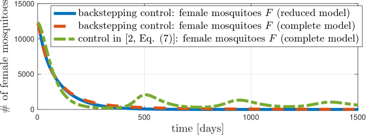
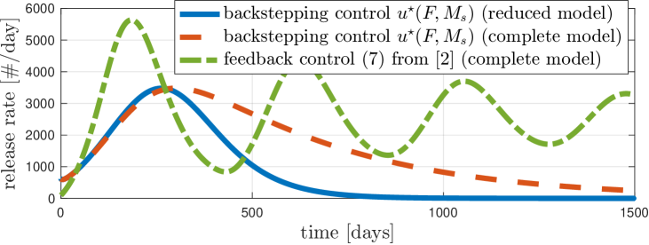
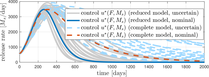
The response of the system to the backstepping control policy is illustrated in the next figures. In particular, Figure 1 shows the evolution of the females: the behaviour of this compartment of mosquitoes population, driven by the control (6)-(8), is quite similar for the reduced model and the complete model, in both cases being characterized by a clear exponential decay. In contrast to such similarity, the behavior of control inputs shows a remarkable difference as visible in Figure 3. In particular, in the case of complete dynamics, the initial behaviour is equivalent to the one of reduced dynamics but then the decay becomes slower, thus indicating that a larger number of sterile males is needed to guarantee the reduction of females when their number decreases. It is also interesting to notice that the control input is vanishing and always non-negative (see Remark 2), thus showing the efficacy of the proposed backstepping approach in driving the female mosquitoes towards the extinction equilibrium.
The obtained results suggest that the feedback control law (6)-(8), although being tailored for the reduced model, is actually applicable with success also for the stabilization of the complete model.
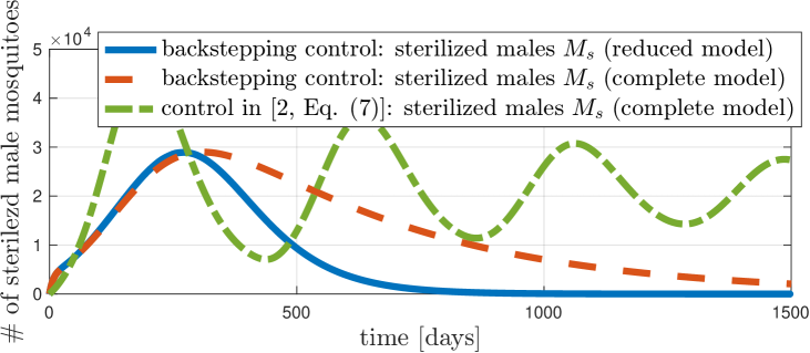
Conversely, it is apparent that the feedback law in [8, Eq. 7], which was specifically designed for the reduced model with optimality purposes, is instead not suitable for the stabilization of the complete system.
In fact, on the one hand, persistency of oscillations is visible in the dashed-dotted plots in Figure 1-2 and, on the other hand, a non-vanishing control behaviour characterizes the dashed-dotted plots in Figure 3.
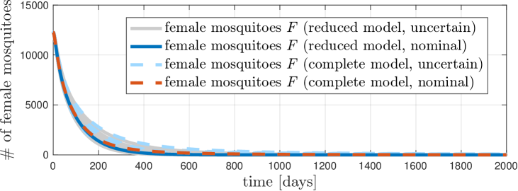
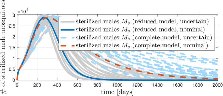
To better illustrate the capabilities of the proposed control law, we have also performed a robustness check. In particular the nominal control law, defined based on the parameter values given in Table 1, has been fed to a system whose parameters were subject to a 10% random uncertainty with respect to the nominal values in Table 1. The results obtained for random iterations, reported in Figures 4-6, are quite promising and support the claim of robustness, with stabilization of the extinction equilibrium for the uncertain system even when the latter is controlled by the nominal feedback law. It is worth noticing that the uncertainty in the model may lead to larger values of the control function compared to the nominal case (see Figure 6). Nevertheless, we can observe that the asymptotically decreasing behaviour of the control is preserved in all the performed iterations. It is also foreseen that better performances are likely to be obtained when the control parameters are selected according to a worst-case choice given a certain bounded range of model uncertainties, thus paving the road for a future formal proof of robust exponential stabilization by means of the proposed backstepping controller.
5 Conclusions and discussion
In this paper we have considered a stabilization problem of the extinction equilibrium for a population of mosquitoes through the sterile insect technique. Using a model-based setup, a backstepping control law has been considered and proved to guarantee the global stabilization of a reduced model comprising females and sterile males only. Sufficient conditions are provided for the non-negativity of the control function, representing the rate of release of sterile males. Furthermore, the same feedback control law has been tested in simulations for the complete model, showing its efficacy for this case too. A preliminary simulation study on the inherent robustness of the proposed backstepping control has been also performed with success, both for the reduced and the complete model. Motivated by the encouraging testing in simulations, currently we are working on enhancing the proposed backstepping control approach by formally considering robustness to uncertainties in the model parameters and in the environmental capacity as previously addressed in, e.g., [16], and introducing sampled measurements, to better catch the typical discontinuities in data acquisition and during the releasing process [17]. Moreover, we aim at formally proving global stability for the complete model under the proposed backstepping controller. Future developments will also be devoted to dealing with diffusion terms in the model, similarly to what has been done in [18], [4],[5], and to consider control based on the incompatible insect technique [19], [20].
References
- [1] E. Knipling, H. Laven, G. B. Craig, R. Pal, J. Kitzmiller, C. Smith, and A. Brown, “Genetic control of insects of public health importance,” Bulletin of the World Health Organization, vol. 38, no. 3, p. 421, 1968.
- [2] A. F. Harris, D. Nimmo, A. R. McKemey, N. Kelly, S. Scaife, C. A. Donnelly, C. Beech, W. D. Petrie, and L. Alphey, “Field performance of engineered male mosquitoes,” Nature biotechnology, vol. 29, no. 11, pp. 1034–1037, 2011.
- [3] V. A. Dyck, J. Hendrichs, and A. S. Robinson, Sterile insect technique: principles and practice in area-wide integrated pest management. Taylor & Francis, 2021.
- [4] L. Almeida, A. Leculier, and N. Vauchelet, “Analysis of the rolling carpet strategy to eradicate an invasive species,” SIAM Journal on Mathematical Analysis, vol. 55, no. 1, pp. 275–309, 2023.
- [5] A. Léculier and N. Nguyen, “A control strategy for the sterile insect technique using exponentially decreasing releases to avoid the hair-trigger effect,” Math. Model. of Natural Phenomena, vol. 18, 2023.
- [6] P.-A. Bliman, D. Cardona-Salgado, Y. Dumont, and O. Vasilieva, “Implementation of control strategies for sterile insect techniques,” Mathematical biosciences, vol. 314, pp. 43–60, 2019.
- [7] L. Almeida, M. Duprez, Y. Privat, and N. Vauchelet, “Mosquito population control strategies for fighting against arboviruses,” Math. Biosci. Eng, vol. 16, no. 6, pp. 6274–6297, 2019.
- [8] ——, “Optimal control strategies for the sterile mosquitoes technique,” Journal of Differential Equations, vol. 311, pp. 229–266, 2022.
- [9] K. Agbo bidi, L. Almeida, and J.-M. Coron, “Global stabilization of sterile insect technique model by feedback laws,” arXiv preprint arXiv:2307.00846, 2023.
- [10] M. Strugarek, H. Bossin, and Y. Dumont, “On the use of the sterile insect release technique to reduce or eliminate mosquito populations,” Applied Mathematical Modelling, vol. 68, pp. 443–470, 2019.
- [11] W. M. Haddad, V. Chellaboina, and Q. Hui, Nonnegative and compartmental dynamical systems. Princeton University Press, 2010.
- [12] B. Ernawan, T. Anggraeni, S. Yusmalinar, H. I. Sasmita, N. Fitrianto, and I. Ahmad, “Assessment of compaction, temperature, and duration factors for packaging and transporting of sterile male aedes aegypti (diptera: Culicidae) under laboratory conditions,” Insects, vol. 13, p. 13, 2022.
- [13] Vector Disease Control International, “Understanding the life cycle of the mosquito.” [Online]. Available: https://www.vdci.net/mosquito-biology-101-life-cycle/
- [14] M. M. Sowilem, H. A. Kamal, and E. I. Khater, “Life table characteristics of Aedes Aegypti (Diptera: Culicidae) from Saudi Arabia,” Tropical biomedicine, vol. 30, no. 2, pp. 301–314, 2013.
- [15] A. Isidori, Lectures in feedback design for multivariable systems. Springer, 2017.
- [16] P.-A. Bliman and Y. Dumont, “Robust control strategy by the sterile insect technique for reducing epidemiological risk in presence of vector migration,” Mathematical Biosciences, vol. 350, p. 108856, 2022.
- [17] K. Agbo bidi, “Feedback stabilization and observer design for sterile insect technique model,” arXiv preprint arXiv:2402.01221, 2024.
- [18] L. Almeida, J. Estrada, and N. Vauchelet, “Wave blocking in a bistable system by local introduction of a population: application to sterile insect techniques on mosquito populations,” Math. Model. of Natural Phenomena, vol. 17, p. 22, 2022.
- [19] Zheng, Xiaoying et al., “Incompatible and sterile insect techniques combined eliminate mosquitoes,” Nature, vol. 572, no. 7767, 2019.
- [20] P.-A. Bliman, “Feedback control principles for biological control of dengue vectors,” in 2019 18th European Control Conference (ECC). IEEE, 2019, pp. 1659–1664.