ShanghaiTech Mapping Robot is All You Need: Robot System for Collecting Universal Ground Vehicle Datasets

Abstract

This paper presents the ShanghaiTech Mapping Robot, a state-of-the-art unmanned ground vehicle (UGV) designed for collecting comprehensive multi-sensor datasets to support research in robotics, computer vision, and autonomous driving. The robot is equipped with a wide array of sensors including RGB cameras, RGB-D cameras, event-based cameras, IR cameras, LiDARs, mmWave radars, IMUs, ultrasonic range finders, and a GNSS RTK receiver. The sensor suite is integrated onto a specially designed mechanical structure with a centralized power system and a synchronization mechanism to ensure spatial and temporal alignment of the sensor data. A 16-node on-board computing cluster handles sensor control, data collection, and storage. We describe the hardware and software architecture of the robot in detail and discuss the calibration procedures for the various sensors. The capabilities of the platform are demonstrated through an extensive dataset collected in diverse real-world environments. To facilitate research, we make the dataset publicly available along with the associated robot sensor calibration data. Performance evaluations on a set of standard perception and localization tasks showcase the potential of the dataset to support developments in Robot Autonomy.

I Introduction

The core contributions of this paper are:

• System paper of very nice SLAM dataset collection robot

• Calibration

• Carachterization

• Dataset with Evaluation

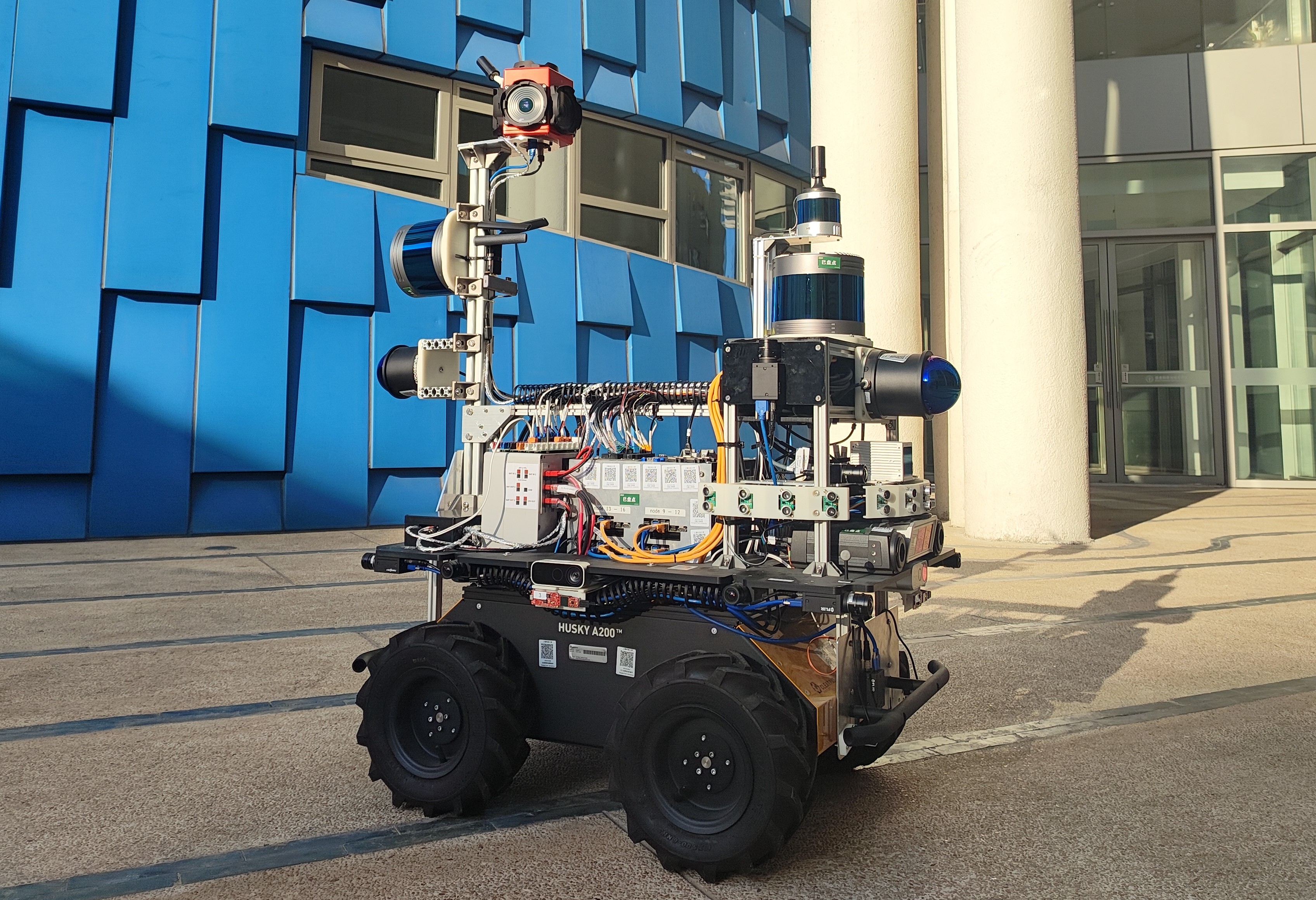
Figure 1: The ShanghaiTech Mapping Robot II.

We are presenting a UGV-based mapping robot capable of accommodating, powering, synchronizing and controlling various kinds of sensors orientated towards multiple directions as well as collecting and storing data from all sensors. The robot is designed to accommodate (i) facing the front direction, a pair of wide-angle color camera, a pair of infra-red camera, a pair of event-based camera, an RGB-Depth camera, a mmWave radar, 2 solid-state non-rotational LiDARs, (ii) facing each of the left, right, back and up direction, a pair of wide-angle color camera, an RGB-Depth camera, a mmWave Radar, (iii) facing downward, one wide-angle color camera, (iv) on the top, an polydioptric omnidirectional color camera (consisting of 6 wide-angle color camera) and 2 real-time kinematic GNSS antennas, (v) surrounding the robot, 5 rotational LiDARs, 13 ultrasound range finder and an AHRS IMU.

The vehicle mechanically consists of the UGV base, structure for sensor mounting, the power box and the computation cluster.

II Related Work

In recent years, several public datasets have been introduced to support research in autonomous driving and mobile robotics. The KITTI dataset [1] is one of the pioneering works that provides synchronized camera and LiDAR data captured from a moving vehicle. The dataset includes RGB images, grayscale stereo images, 3D Velodyne point clouds, and GPS/IMU data.

The Cityscapes dataset [2] focuses on semantic understanding of urban street scenes. It provides stereo RGB images with pixel-level and instance-level semantic annotations for 30 classes. The dataset is captured in 50 different cities during daytime and good weather conditions.

The Oxford RobotCar Dataset [3] introduces a large-scale autonomous driving dataset captured over a year in Oxford, UK. The dataset covers different times of day, weather conditions, and traffic densities. It includes RGB images, 2D LiDARs, 3D LiDARs, GPS/IMU, and RTK ground truth.

More recent datasets such as nuScenes [4], Waymo Open Dataset [5], and Argoverse [6] incorporate richer sensor modalities and provide larger data volumes. The nuScenes dataset includes RGB cameras, LiDARs, radars, and GPS/IMU. Waymo Open Dataset and Argoverse provide high-quality LiDAR point clouds and 3D object annotations.

While these datasets have significantly advanced research in autonomous driving, they are still limited in certain aspects. Most datasets focus on a specific sensor configuration and do not cover the full spectrum of sensing modalities. The calibration quality and synchronization accuracy are often not rigorously evaluated. Most importantly, the diversity of environments and conditions is still limited.

Our ShanghaiTech Mapping Robot seeks to address these limitations by incorporating a more comprehensive sensor suite, ensuring high-quality calibration and synchronization, and capturing data in more diverse environments. The dataset and benchmarks enabled by our robot will complement existing datasets and support new research directions in robot autonomy.

III Fleet of Sensors

Ground vehicles like road automotive, warehouse AGVs, or even household robot vacuum cleaners, all have different sensors equipped by them, suiting their size, environment of operation and budget. Moreover, the choice of sensor is affected by the indented mission of the vehicle. Most vehicles would use the data for basic localization and mapping while some of them also expect fine reconstruction of environment or detecting surrounding objects they try to avoid bumping into (or contrarily, would like to interact with).

Different types of sensors suit different tasks. To achieve the goal of collecting universal ground vehicle datasets, we tried our best to equip our robot with almost all kinds of sensors utilized in SLAM and self-driving field, hoping that the datasets it produce would fit most, if not all, SLAM algorithms. To be specific, our choice covers visual sensors (including frame-based RGB cameras, depth cameras, infra-red cameras and event-based cameras), LiDARs (including rotational ones and solid ones), inertial sensors, mmWave radars, ultrasonic range finders and GNSS receivers. In this section, we will introduce the fleet of sensors on the robot.

III-A RGB Cameras

RGB camera is one of the most used sensor in the SLAM field, providing data for visual SLAM algorithms and occupancy or semantics networks. Conventional algorithms utilize either mono or stereo visual streams. State-of-the-art occupancy networks in auto-driving field even use the bird-eye-view image stitched from surrounding cameras as the only input for the network. Thus we equipped the mapping robot with 2 models of RGB cameras, FLIR Grasshopper3 (GS3-U3-51S5C-C) and FLIR LadyBug5+.

FLIR Grasshopper3 (GS3-U3-51S5C-C) is a 2/3-inch color camera that has a resolution of $2448\times 2048$ pixel and can capture images in global shutter mode at the frame rate up to 75fps.[7] Our initiative was to use them to achieve stereo view towards five main directions: front, back, left, right, up, and to have a monocular downward view of the floor or ground the robot drives on. FLIR LadyBug5+ is a polydioptric omnidirectional color camera, consisting of 6 pinhole cameras. 5 of the cameras face the surrounding while the last one faces upward. Each of the 6 sensors has a resolution of $2464\times 2048$ and a maximum frame rate of 30fps [8].

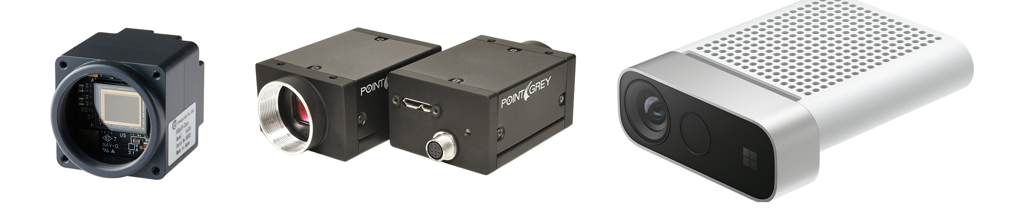
Figure 2: EvC3A event-based camera, FLIR Grasshopper3 (GS3-U3-51S5C-C), and Azure Kienct DK depth camera (from left to right respectively)

III-B RGB-Depth Cameras

Compared to RGB camera that provides no depth measurement, RGB-Depth camera captures both color (RGB) and depth information simultaneously. It combines a standard color camera with a depth sensor, providing a 3D representation of the captured scene.

We chose Azure Kinect DK as the RGB-D camera of our robot. It features a 12MP high-resolution ($3072\times 1920$) RGB camera that can capture color images in global shutter mode at 30fps and an 1MP depth camera that uses ToF technology to measure distance within the range of 0.5 - 5.46 meters [9]. Compared to depth cameras that use structured light technology, ToF RGB-D cameras work better in outdoor environments and have a longer range, which is more suitable for our robot.

We wanted our robot to have multiple Azure Kinect DKs, respectively cover the front, back, left, right, and up direction.

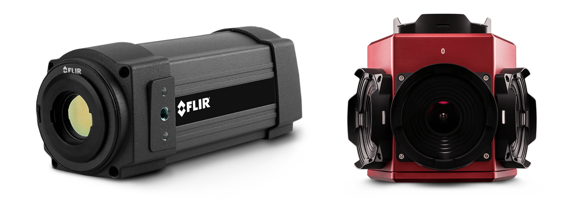
Figure 3: A315 infra-red camera (left) and Ladybug 5+ polydioptric camera (right)

III-C IR Cameras

IR cameras can measure temperature and thus be used to tell heat-emitting objects like human beings, animals, vehicles, etc., from the background. They are also good at detecting fire or malfunctioning electricity equipment.

For our robot, we chose FLIR A315, a compact uncooled microbolometer thermal camera. A315 features a $320\times 240$ pixels Vanadium Oxide detector, having a temperature detection range from -20°C to 120°C with an accuracy up to ±2°C. Its built-in lens provides a 25° field of view and motorized focusing control. It has a spatial resolution of 1.36 mrad and a temperature resolution of 50 mK. Two A315s should be used to form a forward looking stereo pair.

III-D Event-based Cameras

Unlike conventional frame-based cameras, event-based cameras capture asynchronous ’Contrast Detector’ events representing per-pixel brightness changes and report them at real-time, instead of reading out full frames at a fixed rate, which means that event-based cameras can distinguish motion at a very high speed rate, introducing a new approach into the field of visual SLAM.

We equipped the robot with EvC3A event-based cameras featuring the Prophesee PPS3MVCD sensor (often being referred as the Gen3.1 VGA Sensor) also used in the EVK3 camera. It has a resolution of $640\times 480$ on its 3/4” sensor, achieving a typical latency of 200µs and a dynamic range above 120dB. Two of them should be deployed to form a forward looking stereo pair.

III-E LiDARs

LiDAR-based approaches have always, along with their visual counterparts, sat in the center of the field of SLAM. Featuring straightforward capability in range measuring, LiDARs appear on the whole spectrum of ground vehicles, from $500 robot vacuum cleaners to $50,000 road automotive. To produce a universal ground vehicle dataset, LiDARs, many of them, are a must.

In order to diversify the technical methodologies employed by the LiDAR systems and facilitate comprehensive coverage of the sensing area in all directions, we equipped the robot with seven LiDARs, encompassing five distinct models: Robosense Ruby, Robosense Bpearl, Hesai PandarQT, Livox Avia and Neuvition M1.

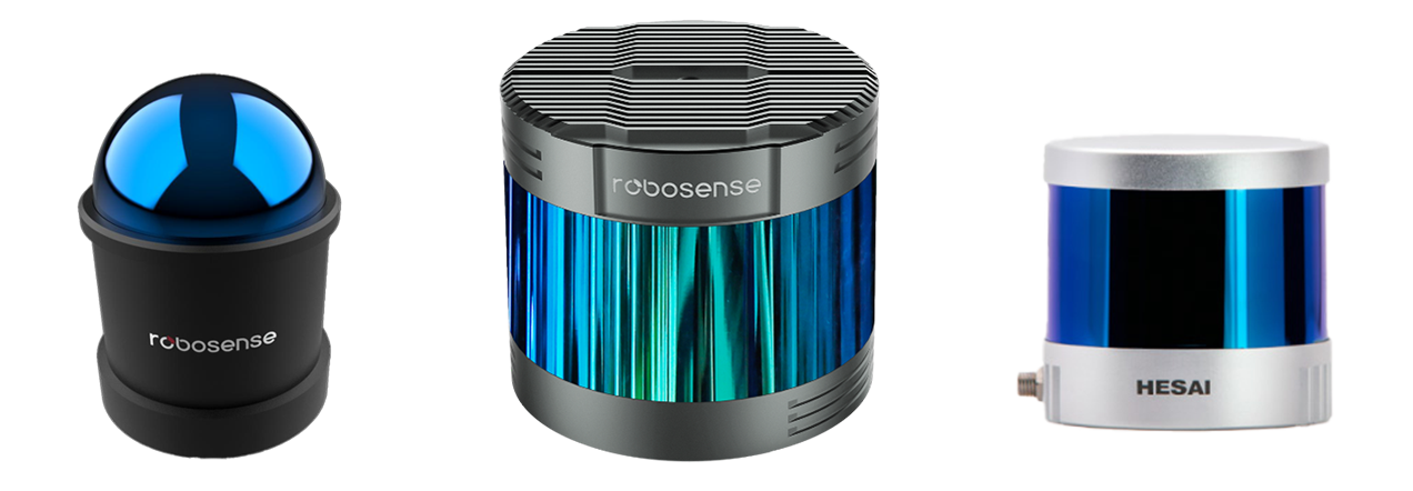
Figure 4: Robosense Bpearl, Robosense Ruby, and Hesai PandarQT LiDARs (from left to right respectively)

Robosense Ruby and Hesai PandarQT are conventional rotational LiDARs. Robosense Ruby is a 128-beam LiDAR with a 0.1° angular resolution on both the horizontal and vertical axes, 200m range and 40° vertical field of view, well-suited for autonomous driving applications requiring far detection range. In contrary, Hesai PandarQT, also known as QT64, is a 64-beam LiDAR designed for indoor applications. It features a 60m range, 0.6° horizontal angular resolution and has a vertical angular resolution up to 1.45°. With a 104.2° (-52.1° to +52.1°) vertical aperture, its FOV covers a typical room from the ceiling to the floor.

Robosense Bpearl is a 32-beam rotational LiDAR featuring a hemispherical $360^{\circ}\times 90^{\circ}$ field of view. It has a small blind range of less than 0.1m and a maximum range of 30m, designed for near-field detection. It provides a vertical resolution of 2.81° and a horizontal resolution up to 0.2°.

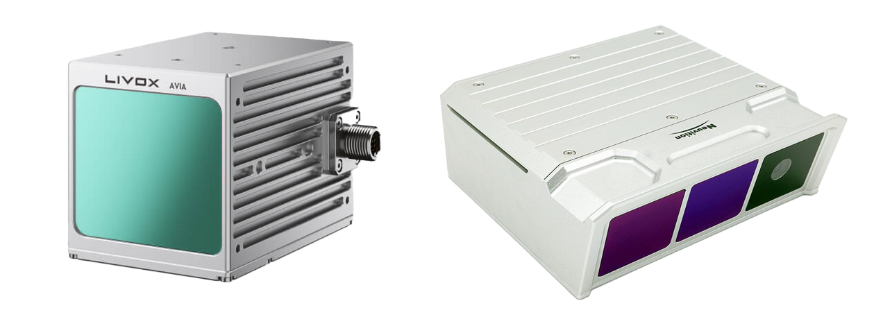
Figure 5: Livox Avia (left) and Neuvition M1 (right) LiDARs

Livox Avia and Neuvition M1 are unconventional LiDARs. Livox Avia is a semi-solid-state LiDAR featuring a unique non-repetitive scanning pattern and a forward-looking field of view. Unlike conventional rotational LiDARs, Livox Avia’s coverage area ratio increases with the time of integration. It has a $70.4^{\circ}\times 77.2^{\circ}$ field of view, 190m range and ±2cm accuracy. It features a best point density among all 5 LiDARs euipped by our robot and thus fits use cases like fine mapping and 3D reconstruction. Neuvition M1 is a MEMS-based solid-state lidar, providing a $45^{\circ}\times 25^{\circ}$ field of view with a $1750\times 480$ resolution and 200m range at 20% reflectivity.

III-F IMUs

Inertial sensors do not rely on signal returned from objects and thus are most environment-adaptive among all kinds of sensors (, geomagnetic and gravitational field do help but are not necessity, let along they are stable at most places on Earth). They can either be used alone for dead reckoning or work with cameras, LiDARs or GNSS receiver to perform multi-sensor fusion localization.

We chose MTi-630R, a rugged and compact attitude and heading reference system (AHRS) from Xsens, to be the main IMU of our robot. It provides 0.2° RMS roll/pitch and 1° RMS heading accuracy and is able to perform high precision strapdown integration at 400Hz. It also measures temperature and atmospheric pressure, potentially helps determine the elevation of robot indoor.

Devices like Livox Avia, Azure Kinect DKs, and the GNSS receiver also have their own built-in IMU.

III-G Ultrasound Range Finders

Ultrasound Range Finders are often equipped by road vehicles for detecting near-field obstacles especially in the context of automatic parking. We equipped our robot with 13 KS103 ultrasonic range finders. KS103 has a range of 1cm to 8m and a resolution of 1cm. It utilizes proprietary filtering techniques to improve ranging accuracy, claiming high precision even in noisy environments.

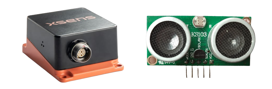
Figure 6: MTi-630R IMU (left) and KS103 ultrasound range finder (right)

III-H mmWave Radars

mmWave Radar is yet another type of sensors that often appears on road vehicles. They can robustly detect the position and relative speed of objects like pedestrians, cyclists, and other vehicles, thus often used to provide functions like Blind Spot Detection and Autonomous Emergency Braking.

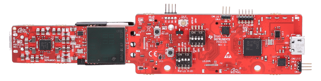
Figure 7: TI IWR6843AOPEVM mmWave Radar

For our robot, we chose IWR6843AOPEVM, a 60GHz mmWave radar from TI. It achieves a wide 120° azimuth and 120° elevation field of view with a small antenna-on-package module. We decided to have five of these radars to look at front, back, left, right, and up directions.

III-I GNSS receiver

To measure an accurate trajectory serving as ground truth in outdoor use cases, GNSS is the best choice. With the assistance of differential reference stations, onboard IMU, and some magic of post-mission processing, GNSS receivers can achieve an accuracy up to 1cm.

We employed a Bynav A1 GNSS RTK receiver that utilizes GPS, GLONASS, Galileo, BeiDou, QZSS, and NAVIC constellations. The receiver supports dual antenna setup, measuring not only the position but also the attitude of the robot. It also has an builtin INS that helps improve positioning both in real-time and for processing afterwards.

IV System Backbone

To make all the sensors mentioned above work simultaneously on our robot, proper data communication, synchronization, powering, as well as an moving base is essential. In this section, we will introduce several main pieces of system hardware acting as the backbone infrastructure of sensing.

IV-A Husky UGV

Our robot is built upon Clearpath Husky, a 990mm long, 670mm wide UGV equipped with rugged construction, high-torque differential drive and lug-tread tires. It has full terrain mobility that allow us to collect datasets in a whole span of various environments, from the interior of buildings, paved roads, to grass fields or even forests.

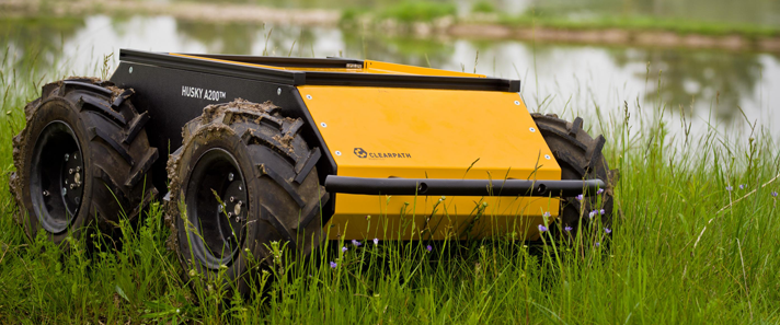
Figure 8: The Clearpath Husky UGV.

IV-B Computation Cluster

To control all the sensors and record the data captured by them, a powerful computer is essential for our mapping robot. [10] Since there are too many sensors on the mapping robot while each of them could capture massive amount of data, even the most powerful portable computer does not have enough I/O and storage bandwidth to handle the recording of data from all sensors. A 16-node computation cluster is specially designed for this usage.

The cluster consists of 16 computing nodes, each modified from an ASUS Mini PN51 computer, having a 8-core, 16-threads Ryzen 7 5700U processor, 32 GiB of RAM, 2 TiB of NVME M.2 SSD storage (Samsung 970EVO Plus, sequential write speed up to 3,300 MB/s), 2 Gigabit Ethernet cards, 3 USB 3.2 Gen1 Type-A ports and 2 USB 3.2 Gen2 Type-C ports. The nodes are stacked in a customized case which also accommodates several DC-DC converters and a LAN switch providing power and interconnection for the cluster, as showed in Fig. 9.

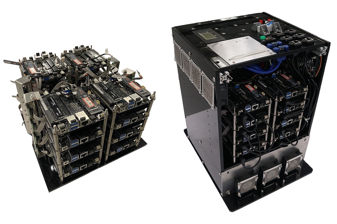
Figure 9: The 16 nodes of the cluster (left) and the complete cluster without one side wall (right).

Among the nodes there is one master node that acts as the controller of the whole cluster while the other worker nodes do not have their operating system install locally but utilize network boot and use the system image hosted on the master node, making it much easier to configure the sensor drivers and orchestration programs over all 16 nodes. This approach also saves storage on worker nodes, allowing a longer record time.

Each worker node is intended to control and record up to 4 sensors, including 3 through USB 3.0 connection and one through Gigabit Ethernet connection. Sensor drivers help configure the sensors connected to the according node and collect the captured data. Raw sensor data will be saved in situ to the SSD mounted on the worker node and can, on demand, be streamed to the master node through ROS. Recorded sensor data can be collected for post-processing by either copying them to external hard drives connected to worker nodes or forwarding them through the master node to an external server.

IV-C Synchronization Board

To eliminate or remedy the time difference of data collected by different sensors, either electronic synchronization or IEEE 1588 PTP (Precision Time Protocol) is the most preferred approach. Both of them can achieve sub-microsecond precision. We employed Syncboard, a combination of Raspberry Pi 4 computer and specially designed I/O shield, to act as a master clock of the whole robot that provides triggering or time base for sensors equipped as well as computation nodes in the cluster. On the Syncboard there are 12 triggering output channels and a LiDAR synchronization channel, capable of connecting at most 130 sensors.

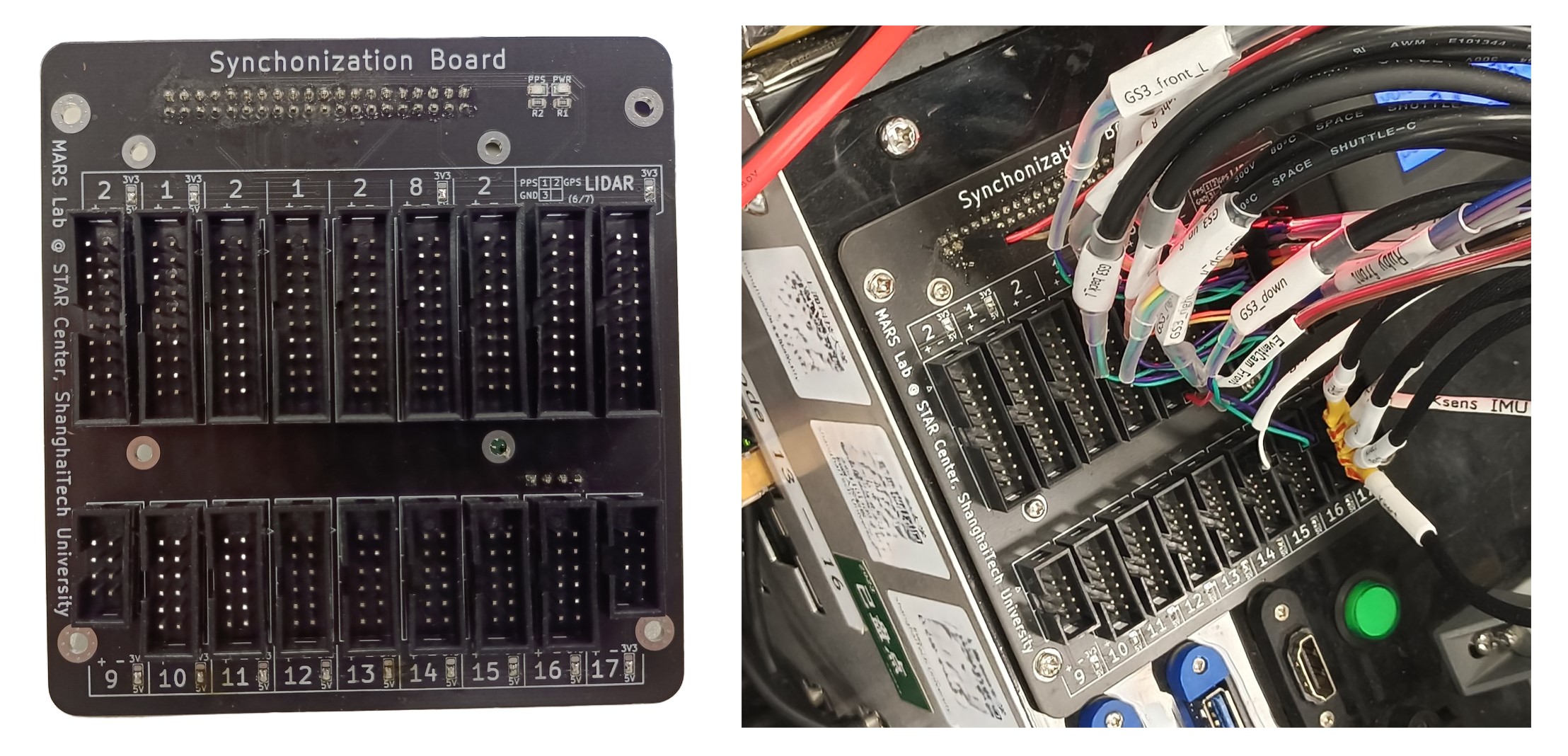
Figure 10: The front side of Syncboard (left). Syncboard installed on the cluster and plugged with triggering cables of sensors (right).

Each of the 12 triggering output channels can generate square wave signals according to the channel-wise designated parameters including frequency (up to 1000Hz), triggering edge polarity (rising edge, failing edge or both edges), time offset and duty ratio, adapting to various triggering-compatible sensors like cameras and IMU. Voltage level of each channel can be set to 3.3V or 5V by changing the soldering bridge on the board. One channel may have 6 to 40 vacancies available for sensor connection, enabling us to easily trigger multiple sensors with the same signal.

The LiDAR synchronization channel, on the other hand, is capable of generating GPRMC+PPS signal. GPRMC, or the Recommended Minimum Specific GPS/Transit Data, is an NMEA 0183 message type designed for carrying positioning data, including a timestamp accurate to the second. It is often given along with a PPS (Pulse-per-Second) signal that indicates the exact beginning of the second contained in the message. Conventional LiDARs consume GPRMC+PPS signal, often from a real GPS receiver in old days, to set their internal clock. The channel can be configured to have certain baud rate as well as an original or inverted voltage level to adapt to different LiDARs. The channel provides 10 vacencies for LiDAR connection.

Nevertheless, Syncboard broadcasts its clock using PTP throughout the cluster LAN such that all computing nodes can synchronize themselves as well as the sensors connected to them. Syncboard itself takes either GNSS or public NTP server as its external master clock.

Syncboard also provides a handy LED button for us to physically start or stop triggering and check its working status, no need to send commands on remote devices.

IV-D Power Box

We designed a power box to provide electricity to all sensors of various types as well as the computation cluster and the UGV base. The power box is able to get power from lithium batteries, convert them into different voltage rails and distributes them to all electric devices.

The power box is equipped with 2 independent battery connectors. High current diodes are employed to isolate the two inputs, enabling the hot swap of batteries and preventing them from charging each other. After flowing through the diodes, electricity meets the main breaker which protects the robot from over-current and acts as the power switch of the robot, then a digital power meter which displays the real-time voltage, current, power, and an integration of energy consumption, before being distributed into converters.

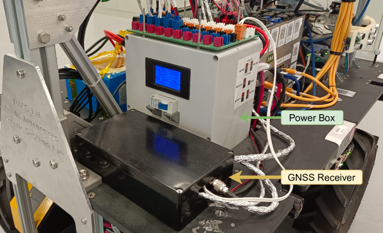
Figure 11: The power box and GNSS receiver of ShanghaiTech Mapping Robot

Inside the power box, multiple DC-DC converters turn the battery power rail into 4 stable DC rails, 5V, 12V, 19V, 24V respectively. The 4 converted rails along side with the battery power rail are connected to the power distribution board, showed in Fig. 12, at the top of the power box. Sensors get electricity from sockets on this board unless they use a single USB port for both data and powering. In that case, they get power from cluster nodes. The UGV base and the computation cluster have their power line connected to the back of the power box to get battery power rail directly.

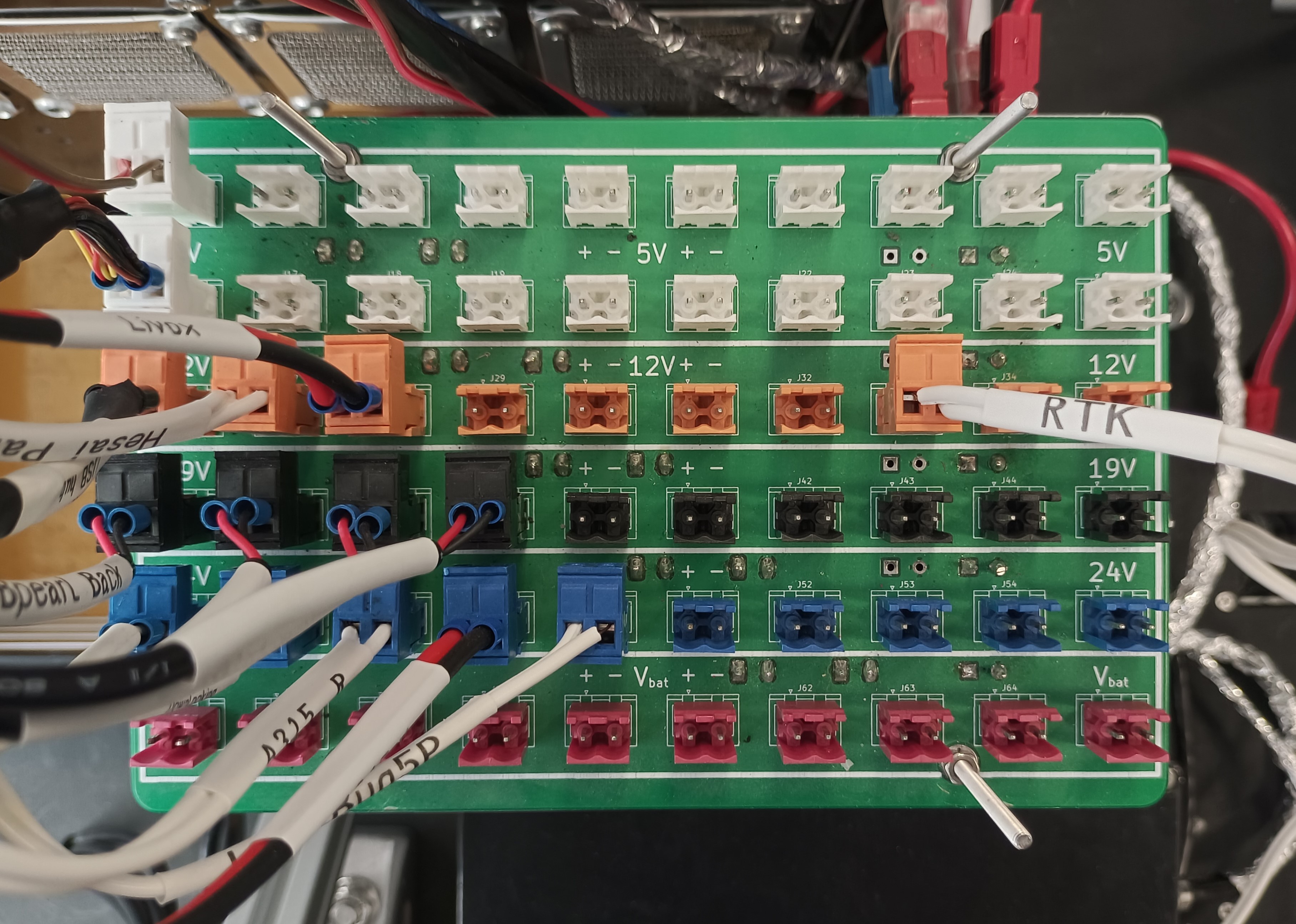
Figure 12: The distribution board at the top of power box. Power lines of several sensors are connected to the box to get electricity of different voltage.

V System integration & Sensor Setup

With all sensors and backbone hardware ready, in this section we will introduce how we integrated all components together as well as the setup of each sensor. As showed in Fig. 13, we designed a sensor deck, a front sensor tower and a back sensor tower to accommodate all sensors

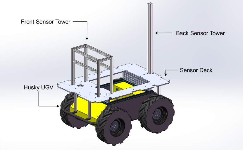
Figure 13: A simple model of ShanghaiTech Mapping Robot II’s mechanical design, showing Clearpath Husky UGV, the sensor deck, front sensor tower and back sensor tower.

V-A Front Sensor Tower

The front sensor tower consists of multiple floors, each of them is made of either aluminum or plastic boards.

On the top there mounts the front GNSS antenna as well as 2 rotational LiDARs, Hesai PandarQT and the first (front) Robosense Ruby.

As showed in Fig. 15 and Fig. 20, PandarQT deserves a position on the very top to observe robot’s near surrounding, including objects at very low angle, with no obstruction. Stayed straight under PandarQT, the front Ruby covers far away objects. Both LiDARs, as well as all rest of them, are connected to separate cluster nodes through Ethernet cable. Each of these nodes handles the control and data collection of the respective LiDAR. Robosense LiDARs are synced using the LiDAR synchronization channel mentioned in Sec. IV-C while LiDARs of other models use PTP protocol to get time base from the syncboard relayed by the cluster nodes.

One floor lower, the first (front) Robosense Bpearl is installed on the front panel. Its zenith of the FoV points forward, providing a hemispherical view of the front of the robot, also showed in Fig. 20.

Behind the front Bpearl, 2 Grasshopper3 cameras, one Azure Kinect DK and a mmWave Radar, showed in Fig. 15 and Fig. 14 are attached on the two side panels and the back panel of this floor. They look upwards and provide a view of ceilings or treetop above. Inside this floor, there stashes the cables and I/O boxes of all LiDARs on the robot.

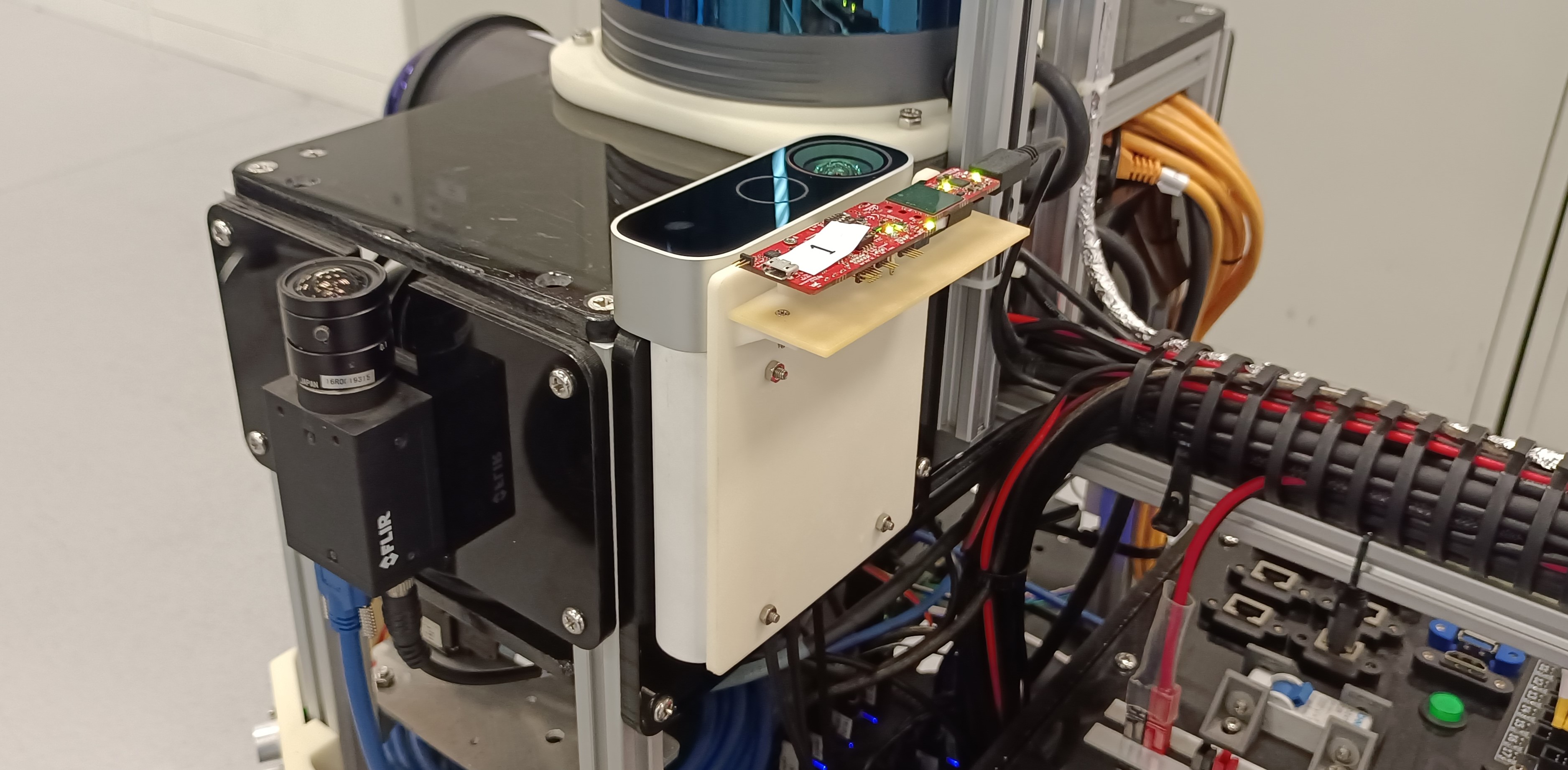
Figure 14: The upward looking Azure Kinect DK and TI IWR6843AOPEVM mmWave radar.

These 2 up-looking Grasshopper3 cameras, as well as their front-, left-, right- and back-looking counterparts, are equipped with Kowa LM6JC wide-angle lenses. It has a focal length of 6mm, providing a wide FoV of $81.9^{\circ}\times 61.2^{\circ}$ and a deep depth of view. [11] We set the focal distance to $\infty$ and aperture to their maximum value of $f/1.4$ to ensure a sharp imaging on far surrounding objects and let sufficient amount of light reach the sensors, enabling high frame-rate capturing. These 10 cameras run in hardware triggering mode and are connected to the same triggering channel on the Syncboard, thus capture images at the same time, with same frame rate.

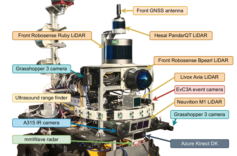
Figure 15: The front sensor tower of ShanghaiTech Mapping Robot II.

Another floor lower, there are 2 EvC3A event-based cameras, MTi-630R IMU, Livox Avia LiDAR, and 13 KS103 ultrasound range finders. The 2 EvC3A event-based cameras form a stereo pair looking forward, using same lenses as Grasshopper3’s. The focal distance setting is of the same but the aperture is set to the smallest since event-based sensors capture the change of brightness instead of the absolute brightness and work better with reasonably limited lighting. The 2 event-cameras synchronize their internal clock with each other using a 1 MHz signal and also receive triggering signals from Syncboard. However, instead of following triggering signals to capture whole frames as frame-based cameras would do, event-based cameras percept them as ’External Trigger’ events which would be stored in the same stream along with ’Contrast Detector’ events mentioned in Sec. III-D.

KS103 ultrasound range finders are installed on curved racks attached to the tower to achieve evenly angled detecting directions. All 13 of them are connected via an I²C bus to a microcontroller which triggers them in an interleaved sequence to avoid cross-talk.

At the bottom of front sensor tower, 2 A315 IR cameras and the Neuvition M1 LiDAR are mounted on the front end of the sensor deck. A315 is equipped with a 18mm lens providing a 25° FoV and has motorized focus motor enabling automatic focusing control. We configured them to output a 16-bit linear temperature image at a frame rate of 60 Hz. They are connected over a Gigabit Ethernet connection to designated cluster nodes that handle their recording and controlling.

At the front of the UGV base, there is a downward looking Grasshopper3 camera, as showed in Fig. 16. Its focal distance is set to match the distance to the ground in order to get a clear view of the floor, road, etc. Alongside it, two 1.5-watt LED lights are installed to ensure enough lighting, enabling a even higher frame rate to compensate for the limited FoV (about $40\times 60$ cm on the ground) due to its low mounting position.

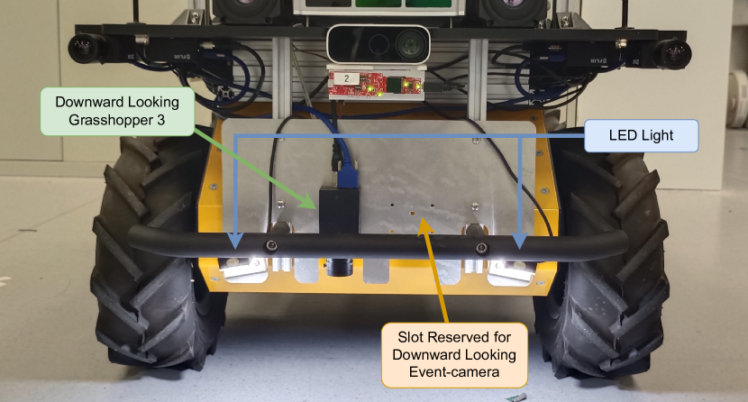
Figure 16: The downward looking Grasshopper3 and LED lights.

V-B Sensor Deck

The sensor deck is made out of one aluminum plate and forms the length and width of the vehicle. It’s mounted directly onto the base UGV by being bolted to the main aluminum extrusion frame around the top of UGV’s payload bay and further supported by aluminum pillars attached to the front and rear bumper bars. Both the front and back sensor tower are attached to the sensor deck. The computation cluster, power box and one out of the 2 batteries are placed through a slot of sensor deck, marked yellow in Fig. 17, onto the UGV’s payload bay.

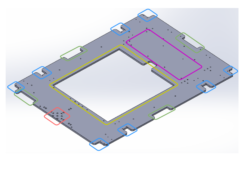
Figure 17: The design of ShanghaiTech Mapping Robot II’s sensor deck. Mounting position for Grasshopper3 (blue), Azure Kinect DK (green), computation cluster (yellow), front sensor tower (purple) and back sensor tower (red).

The sensor deck accommodates the Grasshopper3 cameras, Azure Kinect DK depth cameras and the mmWave radars facing the rest 4 (front, back, left and right) directions. In each direction, the 2 separate Grasshopper3 mounting slots, marked blue in Fig. 17, are capable of aligning the direction and sensor plane of cameras, forming them into a stereo pair.

As showed in Fig. 18, each mmWave radar is mounted on the back of a Azure Kinect DK using a 3D printed part, forming a Kinect-mmWave pair. Such pairs are attached to Kinect mounting slots of sensor deck, marked green in Fig. 17. Such approach insures a uniform translation between all 5 pairs thus helps simplifying the calibration of mmWave radar extrinsics.

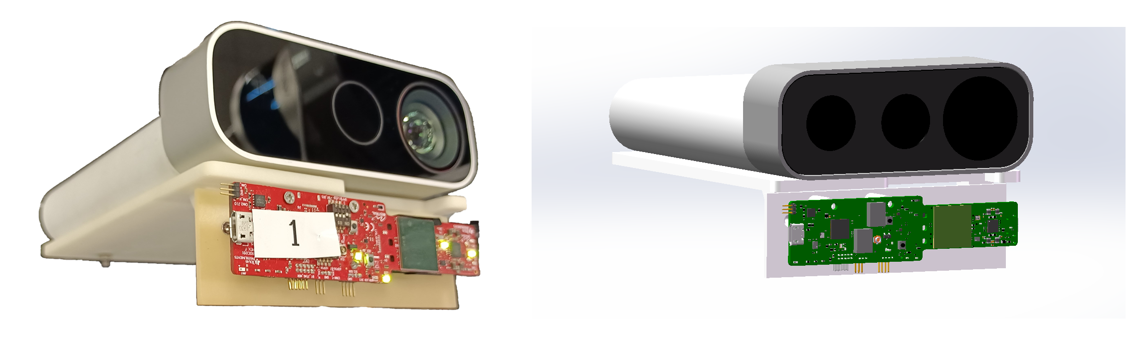
Figure 18: The design (right) and actual photo (left) of 3D printed part connecting Azure Kinect DK and mmWave radar.

The real-time kinematics GNSS receiver is placed on the sensor deck near the back sensor tower. Its 2 antennas are installed atop the front and back sensor tower respectively. The receiver is connected to the cluster LAN and thus has access to online differential corrections data via a 5G cellular link from either local base station or third-party CORS (Continuously Operating Reference Stations) network. It also sends PPS signal to Syncboard via a dedicated cable when acts as an external master clock as mentioned in Sec. IV-C.

The powering, data and synchronization cables of the sensors are routed on the bottom side of the deck.

V-C Back Sensor Tower

The back sensor tower is made out of a single 40mm*40mm aluminum extrusion pillar. Along the pillar there attaches 2 rotational LiDARs, the omnidirectional camera, the rear GNSS antenna as well as WiFi, cellular and joystick receivers.

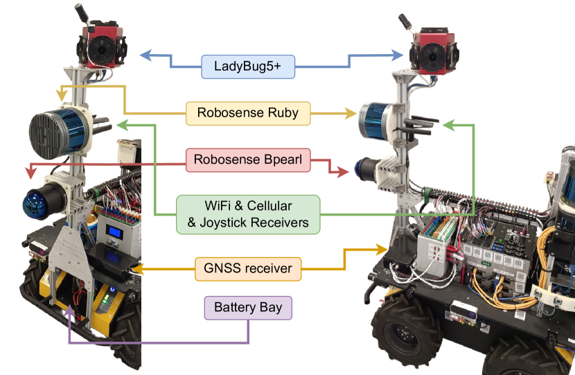
Figure 19: The back sensor tower of ShanghaiTech Mapping Robot II viewed from its back (left) and right (right).

The LadyBug5+ is mounted at the top of the back sensor tower. The built-in lenses of LadyBug5+ have a $f/2.5$ aperture and a 4.4mm focal length, achieving a FoV of 90% full sphere (6 sensors combined) and acceptable sharpness from about 60cm to infinity.[8] We capture original pinhole images from the 6 sensors rather than using its SDK to stitched panorama images on the fly. It is triggered via a dedicated channel of Syncboard. The back GNSS antenna is placed on the top of LadyBug5+ in a particular orientation that hides itself in a blind spot.

At the middle of the back sensor tower there mount the second (back) Robosense Ruby and Bpearl. are installed on the robot. The back Bpearl simply points the zenith of its FoV backwards, opposite to its front counterpart, while the back Ruby is installed vertically, pitched up 90°, achieving a dense vertical scanning and coverage of far objects with high elevation angle like tall buildings along the routes. In Fig. 20, we show the FoV of all 7 LiDARs on the robot.

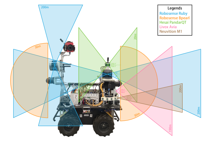
Figure 20: FoV of LiDARs equipped by ShanghaiTech Mapping Robot II.

A USB hub is installed on the back sensor tower to accommodate WiFi, cellular and joystick receivers, providing connectivity to the robot for controlling, monitoring, and access to online reference servers for time and differential GNSS.

Under the back sensor tower, a second battery is installed in the back bay of UGV.

With everything connected, the communication and synchronization architecture of the whole robot are as shown in Fig. 21 and Fig. 22

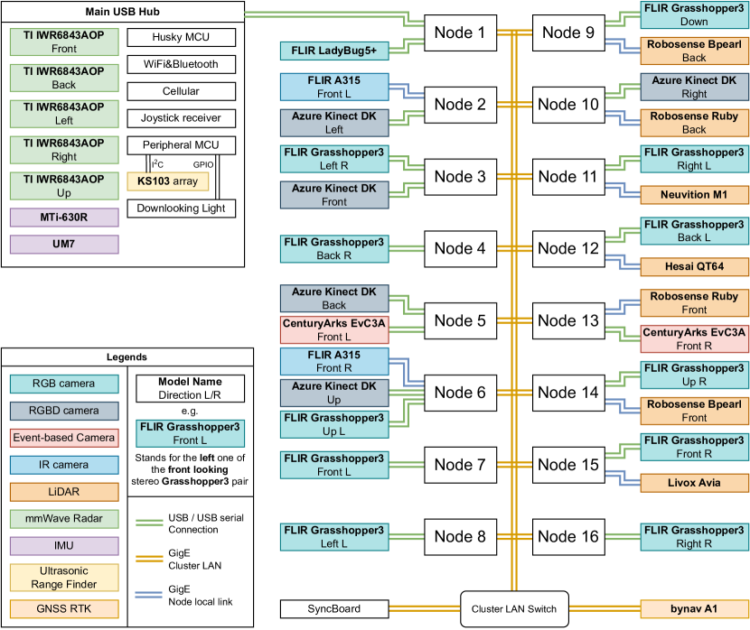
Figure 21: The communication structure of the ShanghaiTech Mapping Robot II.

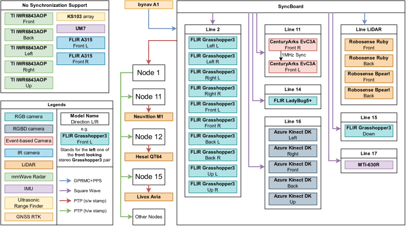
Figure 22: The synchronization flow of the ShanghaiTech Mapping Robot II.

VI Calibration

To ensure accurate perception and mapping, it is crucial to calibrate the intrinsic and extrinsic parameters of the various sensors employed in the system. This section outlines the calibration procedures for the RGB cameras, event-based cameras, and LiDAR sensors.

VI-A Camera Intrinsic & Extrinsic Calibration

The intrinsic and extrinsic parameters of 21 out of the 22 RGB cameras, including 10 Grasshopper3, 5 Azure Kinect DK, and 6 individual sensors of the LadyBug5+, were calibrated using the multi-camera calibration toolbox Kalibr [12] and AprilGrid patterns. Kalibr is capable of calibrating the intrinsic and extrinsic parameters of camera systems with non-globally shared overlapping fields of view and supports various distortion models, such as radial-tangential and equidistant models, which accurately represent the lenses used on the Grasshopper3 and the built-in fisheye lenses on the Ladybug5+, respectively.

For each of the 5 main directions (front, back, left, right, and up), the 2 Grasshopper3s, 1 Azure Kinect DK, and 1 or 2 sensors of the LadyBug5+ facing that side are grouped and calibrated together since they share a similar perspective. This gave us intrinsics of all cameras and 5 extrinsics groups, each independent from the others. Subsequently, the extrinsics between the 5 surrounding LadyBug5+ sensors were calibrated in a separate run, connecting the extrinsics of the 4 horizontal sides (front, back, left, and right). The up-looking side was finally connected to the extrinsic tree using the factory pre-calibrated transformation between the front-looking and up-looking sensors of the LadyBug5+.

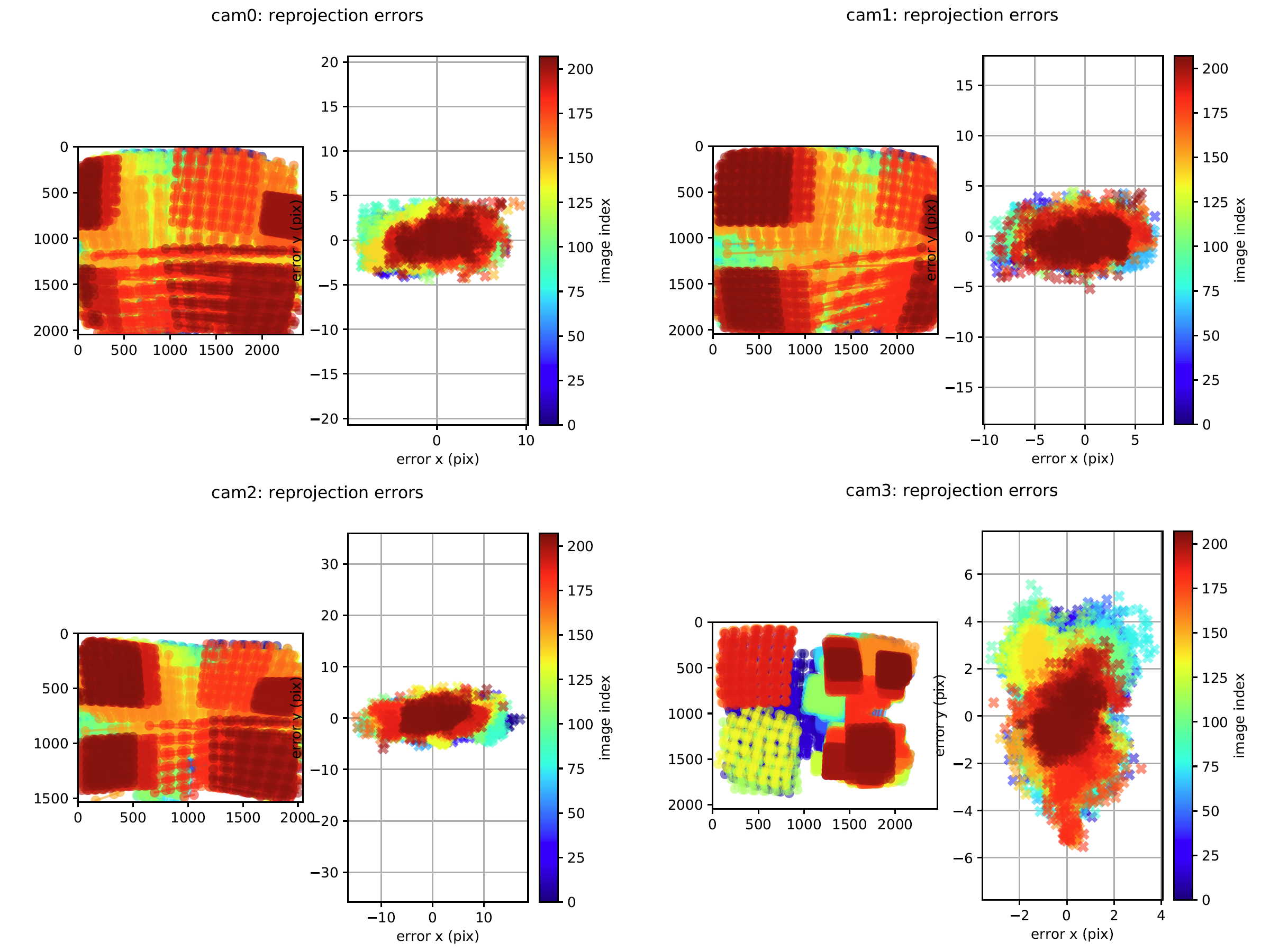
Figure 23: Reprojection error of 4 frontward looking RGB cameras after calibration by Kalibr. (cam0: stereo left Grasshopper3, cam1: stereo right Grasshopper3, cam2: Azure Kinect DK RGB sensor, cam3: LadyBug5+ sensor number 0)

The intrinsic parameters of the last, down-looking Grasshopper3 camera were calibrated using the ROS camera calibration package [13] and a checkerboard target with a size matching the small area of view on the ground. Considering that the camera has no overlapping field of view with any other onboard sensors and that the down-looking image stream is more likely to be used in monocular image registration algorithms rather than visual odometry algorithms, its extrinsic parameters were derived from the structure design instead of using complex calibration algorithms.

The intrinsic parameters of the two EvC3A event-based cameras were calibrated using blinking checkerboard patterns and the calibration tool provided by the Metavision SDK. The extrinsics of the event-cameras were calibrated using Kalibr, utilizing the frame images rendered from the two event streams along with the two image streams captured by the two front-facing Grasshopper3 cameras.

VI-B LiDAR Extrinsic Calibration

The extrinsics between the LiDARs and cameras were calibrated using a combination of LiDAR-Camera and LiDAR-LiDAR approaches. The extrinsic between the front-looking camera of the Ladybug5+ and the Livox Avia LiDAR was estimated using the direct visual-LiDAR calibration toolbox [14]. The Livox Avia’s non-repetitive scanning pattern provides a dense point cloud of the scene in front of the stationary robot, which the toolbox utilizes for accurate direct pixel-level registration with the wide-angle camera image captured by the LadyBug5+.

To calibrate the extrinsics between LiDARs, we registered the scans of each LiDAR against a high-precision scan from a FARO® Focus 3D scanner. The LiDAR scans were captured with the robot standing still and then averaged to reduce temporal noise. The registration algorithm, Iterative Closest Point (ICP) to be specific, yields the transformations between LiDARs. Combined with the camera-LiDAR transformation, all LiDARs were connected to the extrinsics tree.

VI-C Calibration of Other Sensors

The MTi-630R IMU’s Allan Variance parameters, including random walk and bias instability, were calibrated using the allan_variance_ros tool [15]. With the IMU intrinsics, the Kalibr toolbox calibrated the extrinsic between the IMU and the 2 front-looking Grasshopper3 cameras. The mmWave radars on each side share an identical extrinsic with the respective Azure Kinect camera they attached onto, derived from the 3D printed mount’s design. The extrinsics of the ultrasound range finders and other unmentioned sensors were either roughly measured manually or derived from their mounts’ structure design.

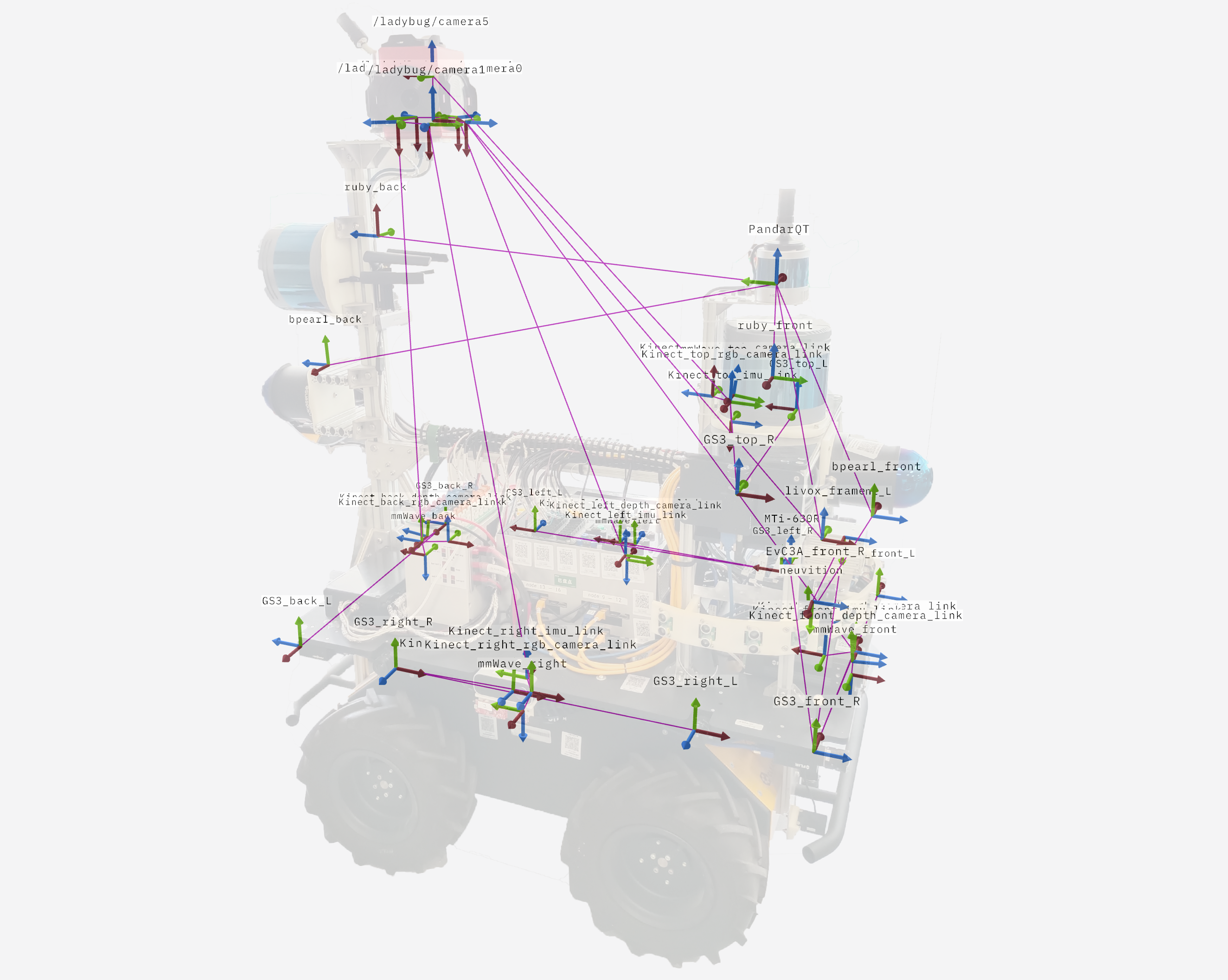
Figure 24: Coordinates of calibrated sensors. Purple lines indicate the edges of transformation tree. An image of mapping robot took from a roughly same perspective is also shown.

VII Procedures and Post-Processing

The mapping robot is designed with distributed computation in mind so it is vital to orchestrate all the nodes in the computation cluster along with the sensors connected to them. In this section we would introduce the procedure of data collection and post-process to be performed on the collected data.

VII-A Procedure of data collection

VII-A1 Material Preparation

At minimum, the robot itself, one battery, and a controlling terminal like KVM or laptop is needed for performing a collection run. A second battery as well as backup ones or power adaptor is recommended.

VII-A2 Power Up

Close the main breaker on the power box. Husky UGV, the master node of the cluster, Syncboard as well as sensors getting electricity from the power box mentioned in Sec. IV-D will be powered up. Following the boot of master node, the robot becomes maneuverable.

VII-A3 Cluster Bringup

The master node sets itself up as the Ethernet gateway and network file systems for Boot-from-LAN, then wakes up all the worker nodes. After they boot, we can control the nodes and access data stored in them. Network access also becomes available for nodes, Syncboard and GNSS receiver.

VII-A4 Time Synchronization

Syncboard gets time base from external master clock and broadcasts it over cluster LAN. We would now perform a manual verification of nodes’ clock, then launch the triggering for sensor test.

VII-A5 Sensors Bringup

The master node orchestrates all worker nodes to launch the sensor drivers. We would manually check if all sensors work as intended. If that’s not the case, sensor’s parameter would be modified accordingly. After everything is confirmed to work well, the triggering is turned off await the upcoming data collection.

VII-A6 Data collection

Command the master node to orchestrate a distributed recording of sensor data. Turn on triggering to officially start a data collection run. We would now drive the robot along the data collection route.

VII-A7 End of collection

After the robot reaches finishing position of the route, the triggering is turned off first, followed by the data recording processes. Sensor drivers stay running and do not have to be spawned repetitively until there is no more data collection runs to be carried out before powering off the robot. The data collected can be copied either into external hard drives via USB port from each nodes or to a workstation or network storage device through Ethernet connection, pending for post-processing.

VII-B Dataset Post-processing

VII-B1 Timestamp Restoration

Replace the timestamps in sensor messages captured by hardware triggered sensors (Grasshopper3 camera, MTi-630R IMU, etc.) with precise triggering time of Syncboard. Any frame drop would be discovered and evaluated at the same time.

VII-B2 Bayer Interleaving

LadyBug5+ on-the-fly compresses each image for the 6 camera sensors in 4 separate Bayer channels using JPEG, resulting in 24 JPEG images per one capture. We decompress and interleave them to get 6 image streams, one sensor each, in bgr8 format.

VII-B3 Image Compression

To provide an alternative compressed version for faster distribution of our dataset, we encode each image stream using AV1 codec.

VII-B4 Mapping Ground Truth

A FARO® Focus 3D scanner is used to obtain a precise point cloud of the environment along the data collection route, acting as the mapping or 3D reconstruction ground truth.

VII-B5 Trajectory Ground Truth

For route sections where GNSS signal stays available, we will post-process the onboard differential GNSS/INS data to obtain a ground truth trajectory with a typical precision of 1cm. Other than that, we register LiDAR scans to the mapping ground truth to get pose of robot as an alternative ground truth for indoor datasets.

VIII Experiments

VIII-A LiDAR&RGBD Interference Evaluation

LiDARs and RGB-Depth cameras on the mapping robot emit infra-red beams and measure the time of flight to obtain distance readings. There are concerns about potential interference between the sensors. In this experiment, we collected point clouds and depth images at a fixed position against a flat, white wall in the basement of ShanghaiTech University with each LiDAR and two RGB-Depth cameras working alone (sole runs) and together (collective run) for 10 seconds, as showed in Fig. 25.

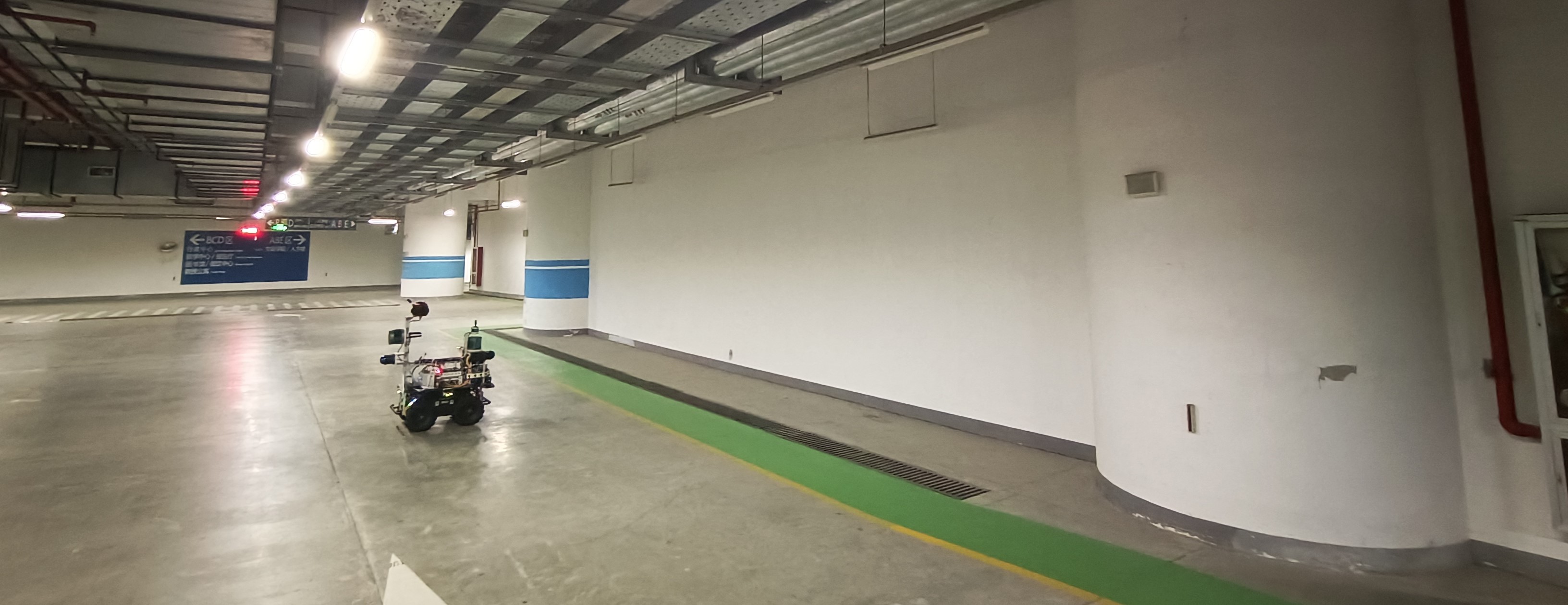
Figure 25: Interference experiment scene setup

VIII-A1 Precision analysis

For rotational LiDARs, the temporal mean and standard deviation of distance measurements for each beam are calculated to indicate the average measurement and precision in respective directions. The mean and standard deviation of the temporal standard deviation among all beams are then computed to indicate overall precision. For unconventional LiDARs (Livox Avia and Neuvition M1), the FOV is binned in elevation and azimuth directions, and the nearest reading in each bin of each ROS pointcloud message is used. For the Azure Kinect depth camera, statistics are performed on each pixel.

$$\overline{D_{b}} =\frac{1}{N_{t}}\sum_{t=1}^{N_{t}}D_{t,b}$$ (1)

$$\sigma_{b} =\sqrt{\frac{1}{N_{t}-1}\sum_{t=1}^{N_{t}}(D_{t,b}-\overline{D_{b}})^{2}}$$

$$\overline{\sigma_{b}} =\frac{1}{N_{b}}\sum_{b=1}^{N_{b}}\sigma_{b}$$

$$\sigma(\sigma_{b}) =\sqrt{\frac{1}{N_{b}-1}\sum_{t=1}^{N_{b}}(\sigma_{b}-\overline{\sigma_{b}})^{2}}$$

Equation 1 is used for calculating the figures for LiDAR precision analysis, where $D_{t,b}$ is the distance measurement of beam or bin $b$ at time $t$, and $\overline{\sigma_{b}}$ is the mean of its temporal standard deviation.

TABLE I: Mean & S.D. of temporal S.D. of distance (m)
Bold figures indicates significant interference

Sensor	Sole $\overline{\sigma_{b}}$ (m)	Collective $\overline{\sigma_{b}}$ (m)	Sole $\sigma(\sigma_{b})$ (m)	Collective $\sigma(\sigma_{b})$ (m)
Robosense Ruby (front)	0.0165	0.0156	0.1961	0.3605
Robosense Ruby (back)	0.0104	0.0104	0.3713	0.3420
Robosense Bpearl (front)	0.0114	0.1719	0.1225	1.4642
Robosense Bpearl (back)	0.0278	0.0690	0.1970	0.8071
Hesai PandarQT	0.0367	0.0373	0.2507	0.2507
Livox Avia	0.0156	2.5236	0.0162	13.9601
Neuvition M1	0.0027	0.0028	0.0025	0.0026
Azure Kinect DK (front)	0.0775	0.1357	0.2511	0.2693
Azure Kinect DK (up)	0.2933	0.3064	0.5330	0.5361

Table I shows that all but the two Robosense Bpearls and the Livox Avia have consistent precision between the sole and collective runs, indicating that the precision of the other LiDARs is not affected by interference.

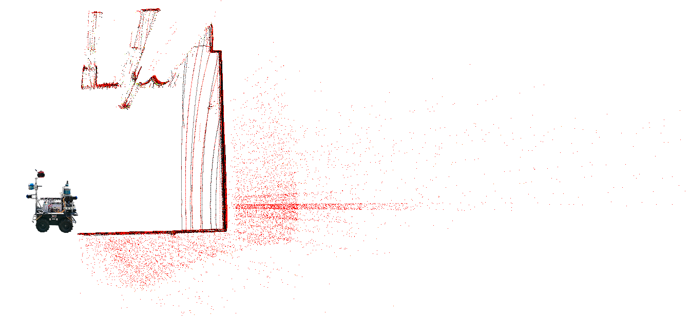
(a) Side perspective

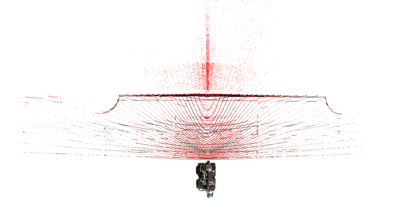
(b) Top down perspective

Figure 26: (a) & (b) Average point cloud produced by front Robosense Bpearl. Black points: sole run; Red points: collective run. The robot thumbnails indicate the approximate position of the robot and do not represent the actual scale.

Fig. 26 (a) & (b) shows the temporal mean of the point cloud collected by the front Robosense Bpearl. In the collective run, both Robosense Bpearl and Livox Avia give noisy points behind the wall or below the floor, indicating interference. However, the non-noisy points have consistent standard deviation of distance compared to the sole run, suggesting that with proper filtering, the two sensors would give point clouds of the same precision regardless of interference.

VIII-A2 Accuracy analysis

To assess the impact on accuracy, the distance between the sensors and a target plane is calculated. Significant changes in this distance would indicate interference-induced accuracy differences. The flat, white wall in front of the robot is used as the target plane for the 5 LiDARs on the front sensor tower, while another flat wall opposite to it is used for the back Robosense Bpearl, and the ground is used for the back Robosense Ruby.

For each sensor, point clouds from the sole and collective runs are merged separately. Points near the target plane are cropped out for accuracy evaluation. A reference plane is fitted to the selected points from the sole run, and the point-to-plane distance $D_{c2p}$ is calculated. The Gaussian distribution of this distance is then fitted for comparison.

TABLE II: Mean & S.D. of Point-to-Plane distance (m)

Sensor	Sole $\overline{D_{c2p}}$ (m)	Collective $\overline{D_{c2p}}$ (m)	Sole $\sigma(D_{c2p})$ (m)	Collective $\sigma(D_{c2p})$ (m)	Rated Accuracy (m)
Robosense Ruby (front, strongest return)	0.0000	-0.0357	0.0219	0.0239	±0.03
Robosense Ruby (front, last return)	0.0000	-0.0020	0.0143	0.0137	±0.03
Robosense Ruby (back)	0.0000	-0.0004	0.0089	0.0088	±0.03
Robosense Bpearl (front)	0.0000	0.0022	0.0131	0.0130	±0.05
Robosense Bpearl (back)	0.0000	0.0009	0.0103	0.0078	±0.05
Hesai PandarQT	0.0000	0.0003	0.0111	0.0108	±0.03
Livox Avia	0.0000	-0.0058	0.0115	0.0115	±0.02
Neuvition M1	0.0000	-0.0029	0.0140	0.0141	±0.02

Table II shows that the difference in point-to-plane distance between the sole and collective runs lies within $2\sigma$ for all LiDARs, indicating no significant accuracy change due to interference.

TABLE III: Pixel-wise Mean & S.D. of Distance Difference(m)

Sensor	$\overline{D_{coll,p}-D_{sole,p}}$ (m)	$\sigma(D_{coll,p}-D_{sole,p})$(m)
Kinect (front)	-0.0057	0.0332
Kinect (up)	-0.0001	0.0840

For depth cameras, the difference in average distance measurements between the sole and collective runs is calculated pixel-wise to detect accuracy changes. As showed in Table III, the mean difference is much smaller than its standard deviation, indicating that the depth cameras’ accuracy is also unaffected by interference.

In conclusion, among all the infra-red light-emitting LiDARs and RGB-Depth cameras on the mapping robot, three give noisy outlier points that can be filtered out using statistical outlier removal approaches. Data from the other sensors along with the inlier data from the aforementioned three sensors have their accuracy and precision unaffected by interference. Except for the up-looking Kinect depth camera and the Hesai LiDAR, the sensors have no mutual sight, possibly preventing inescapable interference as the emitted infra-red laser does not directly shine into the photosensitive sensors of another without reflection from a third object.

VIII-B Demo Dataset

To assess the mapping robot’s data collection capability and verify the compatibility of the collected data with SLAM algorithms, we conducted an outdoor experiment on the ShanghaiTech University campus. The experiment involved collecting data along a predefined route and running SLAM algorithms on the collected data.

VIII-B1 Data Collection

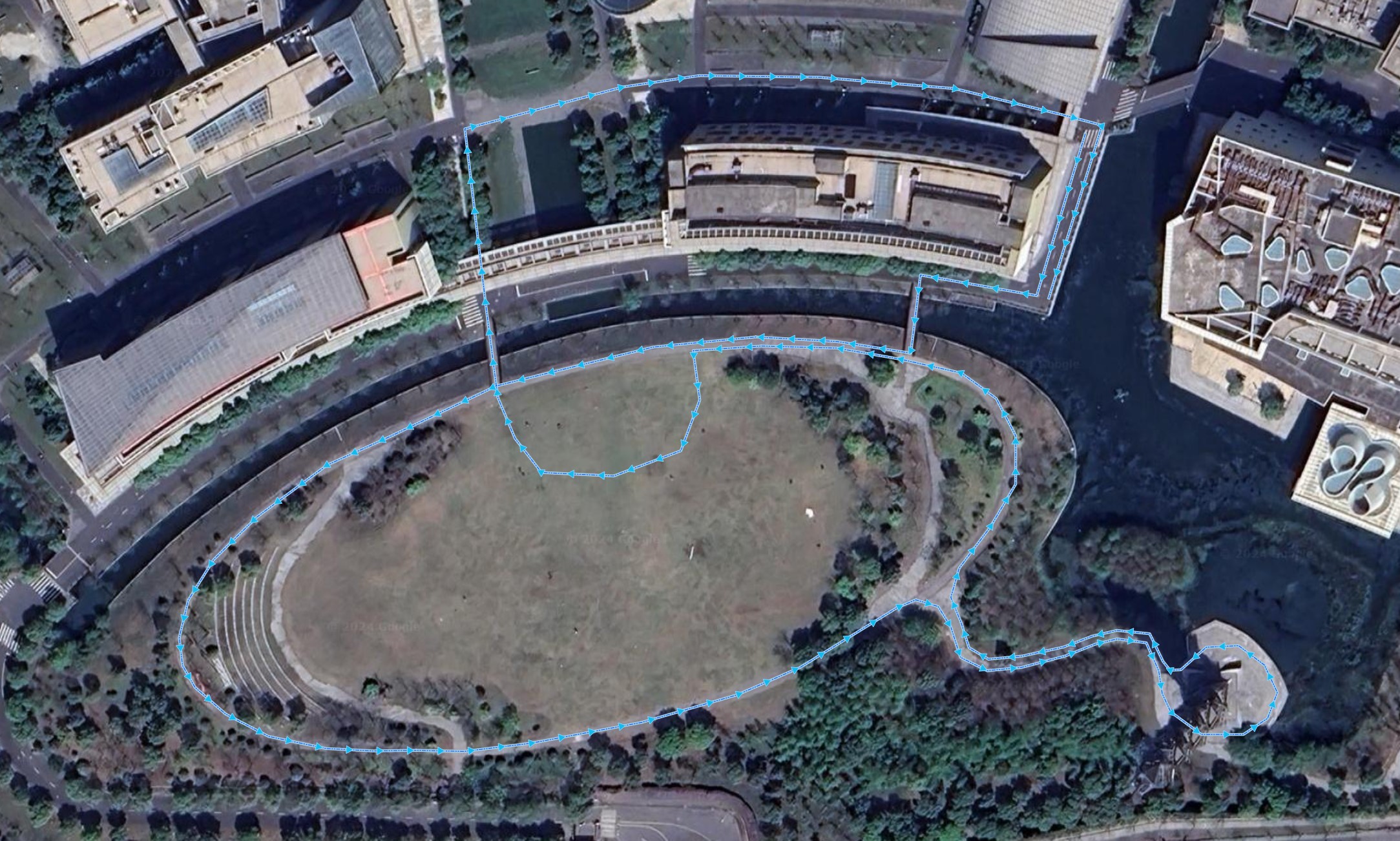
Figure 27: Route plan for outdoor data collection experiment

The 1.4 km data collection route, shown in Fig. 27, was designed to include a variety of terrains and scenes on the ShanghaiTech University campus. The route was evenly split between areas around buildings and parkland, with the mapping robot primarily driving on paved roads or solid structures like bridges, and briefly on grass. Three sections of the route, surrounded by buildings, woods, or a blend of both, were revisited after traveling elsewhere, providing loop-closing opportunities for SLAM algorithms. The route also included slopes to enrich the elevation diversity.

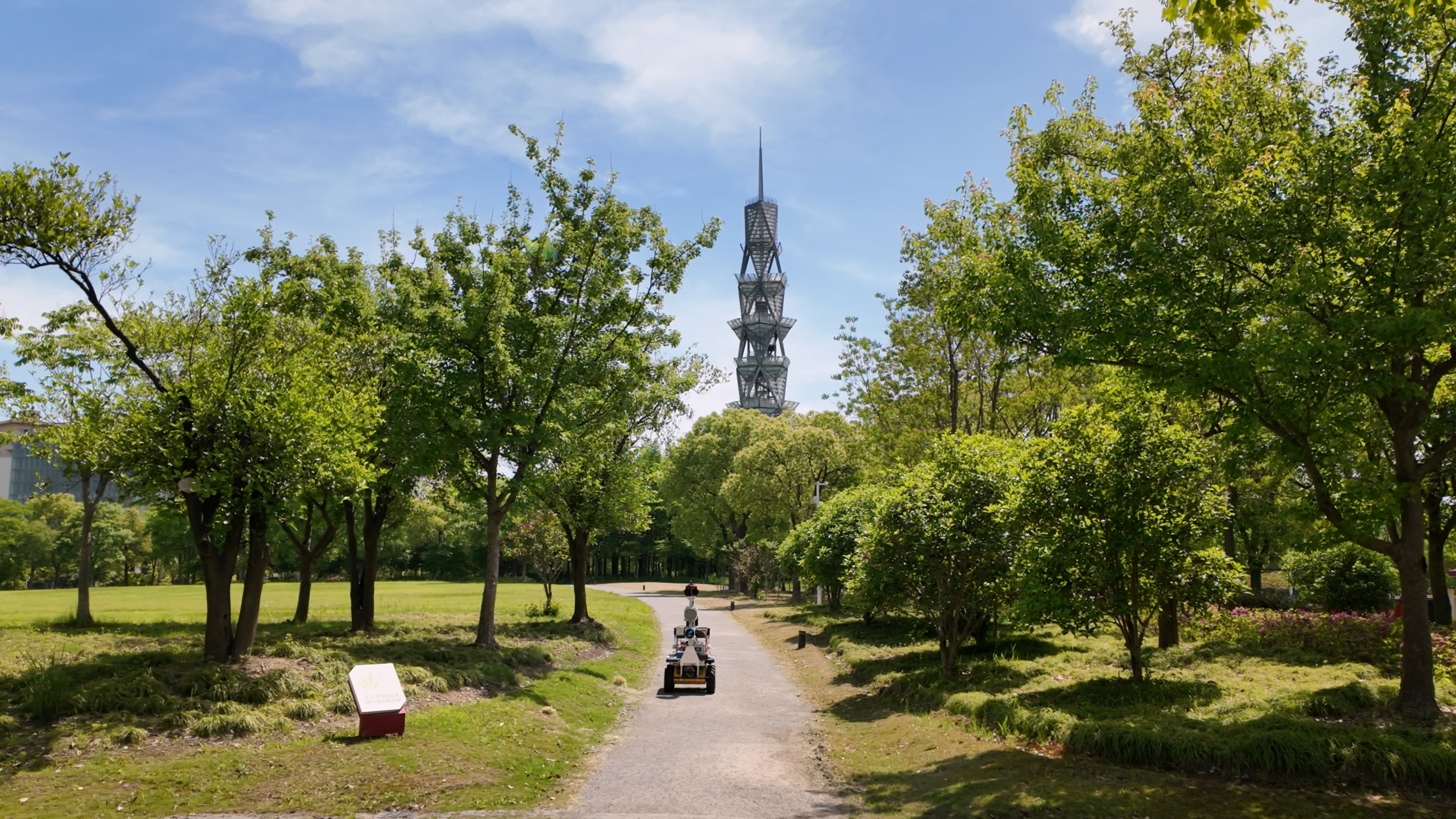
Figure 28: Mapping robot performing data collection on ShanghaiTech campus

The experiment was conducted on an overcast day, providing even lighting on objects and preventing direct sunlight spots in the collected images. The robot took 26 minutes to traverse the entire route, ultimately collecting 2,618 GiB of data, as shown in Fig. 29. A detailed list of the recorded ROS topics is provided in the Appendix.

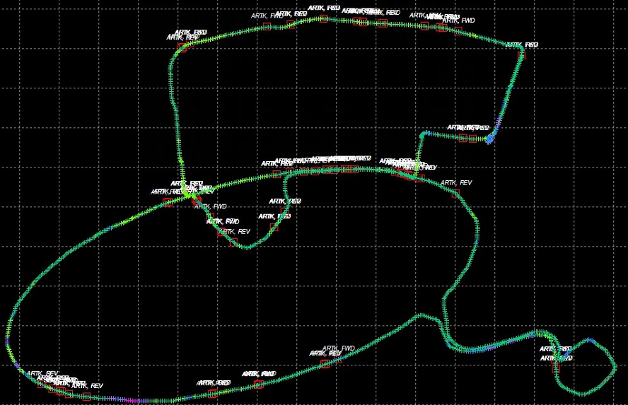
Figure 29: Ground truth trajectory of the experiment run, post-processed from differential GNSS and IMU data

VIII-B2 Lidar-based SLAM

VIII-B3 Visual SLAM

IX Conclusions

Appendix A Details of ROS topics recorded in experiment

References

- [1] A. Geiger, P. Lenz, C. Stiller, and R. Urtasun, “Vision meets robotics: The kitti dataset,” Int. J. Rob. Res., vol. 32, no. 11, p. 1231–1237, sep 2013. [Online]. Available: https://doi.org/10.1177/0278364913491297
- [2] M. Cordts, M. Omran, S. Ramos, T. Rehfeld, M. Enzweiler, R. Benenson, U. Franke, S. Roth, and B. Schiele, “The cityscapes dataset for semantic urban scene understanding,” in 2016 IEEE Conference on Computer Vision and Pattern Recognition (CVPR), 2016, pp. 3213–3223.
- [3] W. Maddern, G. Pascoe, C. Linegar, and P. Newman, “1 year, 1000 km: The oxford robotcar dataset,” The International Journal of Robotics Research, vol. 36, no. 1, pp. 3–15, 2017. [Online]. Available: https://doi.org/10.1177/0278364916679498
- [4] H. Caesar, V. Bankiti, A. H. Lang, S. Vora, V. E. Liong, Q. Xu, A. Krishnan, Y. Pan, G. Baldan, and O. Beijbom, “nuscenes: A multimodal dataset for autonomous driving,” in Proceedings of the IEEE/CVF conference on computer vision and pattern recognition, 2020, pp. 11 621–11 631.
- [5] P. Sun, H. Kretzschmar, X. Dotiwalla, A. Chouard, V. Patnaik, P. Tsui, J. Guo, Y. Zhou, Y. Chai, B. Caine, V. Vasudevan, W. Han, J. Ngiam, H. Zhao, A. Timofeev, S. Ettinger, M. Krivokon, A. Gao, A. Joshi, Y. Zhang, J. Shlens, Z. Chen, and D. Anguelov, “Scalability in perception for autonomous driving: Waymo open dataset,” in 2020 IEEE/CVF Conference on Computer Vision and Pattern Recognition (CVPR), 2020, pp. 2443–2451.
- [6] M.-F. Chang, J. Lambert, P. Sangkloy, J. Singh, S. Bak, A. Hartnett, D. Wang, P. Carr, S. Lucey, D. Ramanan et al., “Argoverse: 3d tracking and forecasting with rich maps,” in Proceedings of the IEEE/CVF conference on computer vision and pattern recognition, 2019, pp. 8748–8757.
- [7] Grasshopper3 usb3 - teledyne flir. [Online]. Available: https://www.flir.com/products/grasshopper3-usb3/?model=GS3-U3-51S5C-C
- [8] Ladybug5+ - teledyne flir. [Online]. Available: https://www.flir.com/products/ladybug5plus/?model=LD5P-U3-51S5C-R
- [9] Azure kinect dk hardware specifications — microsoft learn. [Online]. Available: https://learn.microsoft.com/en-us/azure/kinect-dk/hardware-specification
- [10] Y. Yang, D. Feng, and S. Schwertfeger, “Cluster on wheels,” in 2022 International Conference for Advancement in Technology (ICONAT), 2022, pp. 1–8.
- [11] Kowa 2/3” lm6jc lens. [Online]. Available: https://lenses.kowa-usa.com/jc-series/479-lm6jc.html
- [12] P. Furgale, J. Rehder, and R. Siegwart, “Unified temporal and spatial calibration for multi-sensor systems,” in 2013 IEEE/RSJ International Conference on Intelligent Robots and Systems, 2013, pp. 1280–1286.
- [13] camera_calibration - ros wiki. [Online]. Available: https://wiki.ros.org/camera_calibration
- [14] K. Koide, S. Oishi, M. Yokozuka, and A. Banno, “General, single-shot, target-less, and automatic lidar-camera extrinsic calibration toolbox,” in 2023 IEEE International Conference on Robotics and Automation (ICRA), 2023, pp. 11 301–11 307.
- [15] Allan variance ros. [Online]. Available: https://github.com/ori-drs/allan_variance_ros