Measuring the matter fluctuations in the Local Universe with the ALFALFA catalog

Abstract

The standard model of cosmology describes the matter fluctuations through the matter power spectrum, where $\sigma_{8}\equiv\sigma_{8,0}\equiv\sigma_{8}(z=0)$, defined at the scale of $8\,h^{-1}$ Mpc, acts as a normalisation parameter. Currently, there is a notable discrepancy in the reported values of $\sigma_{8}$ obtained from cosmic microwave background and large scale structure data analyses, which indicates a $\sim 3\,\sigma$ tension between these measurements. This study quantifies matter fluctuations in the Local Universe using HI extragalactic sources mapped by the ALFALFA survey to test the standard cosmological model under extreme conditions in the highly non-linear Local Universe, $z\approx 0$, quantifying the amplitude of the matter fluctuations there, $\sigma_{8}$. Our work directly measures $\sigma_{8}$ using the ALFALFA data, where 3D distances were obtained without assuming $H_{0}$, resulting in a robust model-independent analysis. Our methodology involves the construction of suitable mock catalogues to simulate the large scale structure features observed in the ALFALFA data, applying the 2-point correlation function, and making use of Markov Chain Monte Carlo methods to estimate the parameters. Analysing these data we measure $\sigma_{8}=0.78\pm 0.04$ for $h=0.6727$, $\sigma_{8}=0.80\pm 0.05$ for $h=0.698$, and $\sigma_{8}=0.83\pm 0.05$ for $h=0.7304$, this because a $H_{0}$ value is needed to compare our primary measurement, obtained with the scale in Mpc units, to measurements expressed in $h^{-1}\,\text{Mpc}$ units. Considering the data pairs $(\sigma_{8},H_{0})$ from the Planck CMB and ACT CMB-lensing analyses, our measurement agrees with them in less than $1\,\sigma$ confidence level. From a model-independent perspective, we find that the scale where the matter fluctuation is $1$, is $R=7.2\pm 1.5~{}\text{Mpc}$.

Keywords cosmological parameters from LSS  $\cdot$ power spectrum  $\cdot$ cosmic web

1 Introduction

Cosmic structures form by gravitational instability, when matter contained in a sufficiently dense region collapses. The standard cosmological model reproduces quantitatively the main features of the evolution of matter fluctuations through the matter power spectrum. The normalisation parameter of this spectrum, $\sigma_{8}\equiv\sigma_{8,0}$, is defined as the amplitude of the matter fluctuations at redshift $z=0$ (Peebles, 1967; Feldman et al., 1994; Padmanabhan, 1993; Mo et al., 2010).

A current tension in the value of $\sigma_{8}$ is reported in the literature due to the different values obtained using cosmic microwave background (CMB) and large scale structure (LSS) data (Nunes & Vagnozzi, 2021; Abdalla et al., 2022). Notice that the Planck CMB value, $\sigma_{8}^{\text{Pla}}$, is not a direct measurement but a derived one, assuming the $\Lambda$CDM model to describe the evolution of the primordial perturbations, and using Bayesian analyses to best-fit the CMB temperature fluctuations and combining these data with other cosmic probes. As well, the literature reports $\sigma_{8}$ values obtained through statistical analyses that combine cosmological probes using, sometimes, a model-dependent approach to obtain $\sigma_{8}$ (Planck Collaboration et al., 2020; Heymans et al., 2021; Avila et al., 2022; Madhavacheril et al., 2024).

The cosmological parameter $\sigma_{8}$, that quantifies the matter fluctuation, is related to $\sigma_{8}^{\text{tr}}$, the fluctuation of the cosmic tracer, through a linear bias; $\sigma_{8}$ is used to normalise the matter power spectrum, therefore it is a very important parameter in modern cosmology (Kaiser, 1988; Juszkiewicz et al., 2010). In general, measurements of $\sigma_{8}$ in redshift surveys use cosmic objects that are reliable matter tracers, i.e., $b\sim 1$. By measuring the variance of the number density of galaxies, one effectively obtains the variance of matter, enabling a comparison with diverse measurements reported in the literature (Borgani et al., 1995). The fluctuation in the number density of galaxies in the Local Universe is roughly of order 1 on scales of $8\,h^{-1}$ Mpc ($h$ is defined by $H_{0}=100\,h$ km s^-1 Mpc^-1).

Using Counts-in-Cells (CIC) in the IRAS survey, Efstathiou et al. (1990) found $\sigma^{2}=0.26$ at the effective distance $R=30h^{-1}$ Mpc  and  $\sigma^{2}=0.21$ at $R=40h^{-1}$ Mpc, in disagreement with the prevailing standard cosmological model of that time, i.e., the Cold Dark Matter (CDM) with $\Omega=1$, suggesting that the analysed data exhibited more clustering than predicted by the model. In a later study, Efstathiou (1995) revisited this technique with two surveys of IRAS galaxies found a better agreement with the CDM model. However, taken into account the margin of error, other models were also conceivable, such as those with lower values of the matter density parameter, such as the $\Lambda$CDM model. Simultaneously, Borgani et al. (1995) conducted an extensive work to validate simulated catalogues in the study of cluster distribution, employing various statistical methods to measure $\sigma_{8}$. The application of this methodology to the Abell/ACO cluster redshift sample showed a preference for the $\Lambda$CDM model in explaining Abell/ACO data clustering. More recently, Repp & Szapudi (2020) applying the CIC approach in the SDSS Main Galaxy Sample, constrained $b$ and $\sigma_{8}$ simultaneously, obtaining values of $b=1.36\pm 0.14$ and $\sigma_{8}=0.94\pm 0.11$, which agrees well with previous findings. Overall, these studies indicate that at scales close to or above $8\,h^{-1}$ Mpc, the clustering of galaxies is in excellent agreement with linear perturbation theory, provided that the bias is approximately 1.

The aim of this study is to analyse the mass fluctuations within the Local Universe across several scales, for this we use as a cosmic tracer the HI extra-galactic sources mapped by the ALFALFA survey, and consider cosmic objects with distance from us in the range $20-85$ Mpc. The main motivations to perform this study are: (i) To test the standard cosmological model at extremely low redshift, which means that we are dealing with non-linear scales. In fact, it is well known that the Local Universe exhibits significant non-linear fluctuations in structure growth, providing a unique opportunity to assess the limit of linear theory across various scales (Borgani et al., 1995; Martin et al., 2012; Papastergis et al., 2013; Avila et al., 2018, 2019, 2021; Franco et al., 2024); for this task we use cosmological distances in real space. Indeed, the ALFALFA catalogue offers distance measurements performed independently of assuming a cosmological model, enabling a more direct exploration of spatial relationships (Haynes et al., 2018). (ii) Because the HI sources are effective tracers of dark matter for scales below $10\,h^{-1}$ Mpc (Martin et al., 2012; Papastergis et al., 2013), studying the ALFALFA catalogue, valuable insights into the matter fluctuations in the Local Universe can be obtained. Observe that $\sigma_{8}$ is an important cosmological observable that helps to understand the role of dark matter in the dynamics of cosmic structures growth (Avila et al., 2022). Our analyses differs from others in that: (i) we perform a direct measurement of $\sigma_{8}$ using the ALFALFA survey data in the Local Universe, $z\approx 0$; (ii) we measure $\sigma_{8}$ for HI extra-galactic sources, which are good tracers of matter because $b\sim 1$ (Obuljen et al., 2019); (iii) we use cosmography to measure 3-dimensional (3D) distances, therefore our analysis is model independent; (iv) we perform diverse robustness tests to confirm the validity of our results.

Our work is structured as follows: the ALFALFA catalogue is presented in section 2, which details the process of selecting objects for analyses, as well as the construction of the random catalogues and of the covariance matrix, essential components for our analyses. In section 3, we elaborate on the methodology used to calculate the matter fluctuations, $\sigma(R)$, and its corresponding error. The results of our analyses and our conclusions are presented in sections 4 and 5, respectively. All robustness tests that support our main results are presented in the appendix.

2 The ALFALFA catalogue

The ALFALFA survey was initiated in 2005 with the scientific aim of obtaining measurements of the mass and luminosity functions through extragalactic sources in the 21 cm line. By its conclusion in 2018, it covered an area in the sky of around $6900\deg^{2}$ at redshift $z<0.06$. At the end, $31502$ HI sources were observed. Due to the limitations of the radio telescope used to detect the HI sources, the observations were divided between the northern hemisphere ($7^{h}20^{m}<$ RA $<3^{h}15^{m}$) and the southern hemisphere ($7^{h}20^{m}<$ RA $<21^{h}30^{m}$).

The ALFALFA data show a significant distinction based on the signal-to-noise ratio, categorising them by specific codes: Code 1: involves observations with high signal-to-noise ratio, confirmed in the optical part; Code 2: refers to sources with low signal-to-noise ratio, confirmed in the optical part but considered unreliable; Code 9: relates to high-velocity HI clouds without optical confirmation. In this work, we exclusively use Code 1 sources, following Haynes et al. (2018) (for large-scale structure analyses using the ALFALFA survey see, e.g., Avila et al. (2018, 2021); Franco et al. (2024)).

2.1 Data selection

The distances in the ALFALFA catalogue were measured using two distinct methods: (i) for sources with $cz_{\odot}>6000$ km/s, the distance is estimated using the Hubble-Lemaître law $cz_{\text{CMB}}/H_{0}$, where $cz_{\text{CMB}}$ represents the recession velocity of the galaxies measured in the CMB reference frame; and (ii) for sources with $cz_{\text{CMB}}<6000$ km/s, the distances are calculated using a model for the peculiar velocity field (Masters, 2005), in addition to the use of the Tully-Fisher relation  (Tully & Fisher, 1977). Consequently, we apply a cut removing the distance and velocity range that were calculated using the Hubble-Lemaître law.

One observes a notable concentration of objects around 20 Mpc in the ALFALFA sample, suggestive of the presence of the Virgo Cluster (see, e.g., figure 2 in ref. Avila et al. (2021)). This cluster hosts approximately 224 galaxies and has the potential to introduce systematic effects in our analysis, as the estimated distance is not realistic. Consequently, the mass calculations for the objects belonging to Virgo may be underestimated, highlighting the need to exclude these objects. Moreover, it is expected that the peculiar velocities of galaxies at distances less than $20~{}\text{Mpc}$ are considerably higher, likely due to the strong interaction with the cluster. Therefore, we consider only distances in the range of $20-85$ Mpc with $cz_{\odot}<6000$ km/s (Avila et al., 2023).

The ALFALFA survey was subdivided into observations conducted in the northern and southern hemispheres. In this work we analyse the region in the northern hemisphere, which covers a larger area and encompasses a greater number of detected HI sources. Figure 1 shows the distribution of this sample, while figures 2 and 3 illustrate the footprint and the Cartesian projection of the selected sample, respectively.

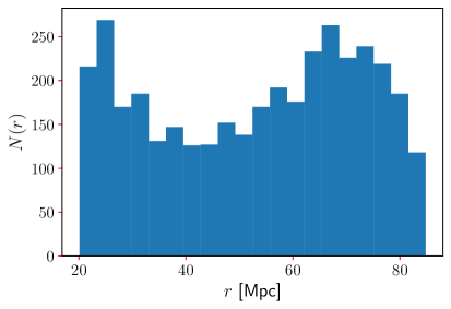
Figure 1: Distances distribution of the selected sample.

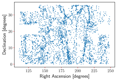
Figure 2: Footprint of the selected sample in equatorial coordinates, localised in the Northern Hemisphere.

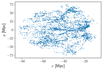
Figure 3: Cartesian projection of the selected sample.

2.2 Random catalogues

The construction of random catalogues, i.e., a point distribution with the same observational features as the data but without correlations between the objects, is an essential step in obtaining the correlation function, $\xi(r)$. The number density of this catalogue is tens of times greater than the sample data in order to reduce the statistical noise in the correlation function (Keihänen et al., 2019; Avila et al., 2024).

For this work, we implemented the publicly available code randomsdss, which allows us to generate a random redshift distribution from the original measurements while keeping the selection features unchanged. The angular distribution is generated following the algorithm from Franco et al. (2024). The random catalogue has ten times as many points as the data sample. Figures 4 and 5 show the angular coordinates and the Cartesian projection of the random catalogue, respectively.

Figure 4: Footprint of the random sample.

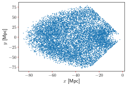
Figure 5: Cartesian projection of the random sample with the footprint of the sample in analysis (see figure 3).

2.3 Mock catalogues

The large-scale structure of the universe is better understood knowing the correlation between its components, information that is encoded in the covariance of the 2-point correlation function of cosmic objects, like the galaxies. In fact, this function encodes crucial information regarding a galaxy survey, including the survey volume, masking effects, and the average galaxy density (see, for instance, ref. de Santi & Abramo (2022)). Calculating the variance of the correlation function needs the evaluation of high-order correlations, however, accurate and accessible methods have been created to estimate it. Reference Martinez & Saar (2001) showed six of such methods, made for specific estimators. These methods usually use either theoretical ideas or the observed galaxy distribution itself to calculate the error, like jackknife and bootstrap techniques (Norberg et al., 2009). Nevertheless, the best method found by Martinez & Saar (2001) uses artificial galaxy distributions, either with N-body simulations or random methods with a known correlation function; it works better because one can obtain the dispersion from multiple correlation function measurements calculated in a way similar to that observed in the sample under analysis.

In this study, we adopt a stochastic model known as Cox processes (Martinez et al., 1998; Pons-Bordería et al., 1999). While this model does not encompass all the non-linear physical processes involved in structure formation, as seen in N-body simulations (Pandey, 2010), Cox processes are advantageous due to their simplicity, low computational requirements, and the availability of their analytic 2-point correlation function (Martinez & Saar, 2001; Avila et al., 2018),

$$\xi_{\text{Cox}}(r)=\frac{1}{2\pi r^{2}L_{V}}-\frac{1}{2\pi r\,l\,L_{V}}\,,$$ (1)

where $l$ and $L_{V}$ are parameters of the point process generation. These mock catalogues are constructed in the following way: we distribute $n_{s}$ segments of length $l$ in a cube of side $L$. The average number of segments per unit volume, $\lambda_{s}$, times the length $l$ defines the density of segments, $L_{V}=\lambda_{s}l$. The number of points on each segment are on average the same. Let $\lambda_{l}$ be the number of points per unit length, then the intensity of the point process is $\lambda=\lambda_{l}L_{V}$.

Due to the methodology of our analyses, we seek that the correlation function obtained from the Cox processes be close to the correlation function of the HI sources. The dispersion of the $n$ realisations, described above, will represent the error of the correlation function of the sample of HI sources. Thus, the parameters of the Cox process are adjusted in such a way as to reproduce the observational features presented by the sample in analysis. However, an initial step can be taken by assuming the Cosmological Principle: on sufficiently large scales the universe is statistically homogeneous and isotropic. This imposes restrictions on the values of $l$. It can be shown that the scale of homogeneity in the Cox process is $R=4\,l$. Assuming a minimum scale for homogeneity of 100 Mpc, one expects $l>25$ Mpc. Our procedure starts fixing $l=25$ and then chose $L_{V}$ when getting a number density similar to our HI sample.

For this work, we set the following values for the Cox process parameters: $\{l,L_{V},\lambda_{l}\}=\{25,0.008,1.8\}$. To obtain a representative dispersion, we construct 1000 mocks. In the figures 6 and 7, we show an example of a realisation of a Cox process in angular coordinates and its Cartesian projection, respectively. Visually, a realisation from the Cox process appears more clustered on small scales. This is because, in order to obtain good agreement on the scales analysed, it was necessary to increase the average number of points on the randomly distributed segments. As we are not analysing a large cosmological volume, we do not observe the correlation function of the HI sources going to zero, and consequently it is difficult to correctly adjust simultaneously all the scales of the Cox process, as $l$ indicates the scale where the equation (1) is zero.

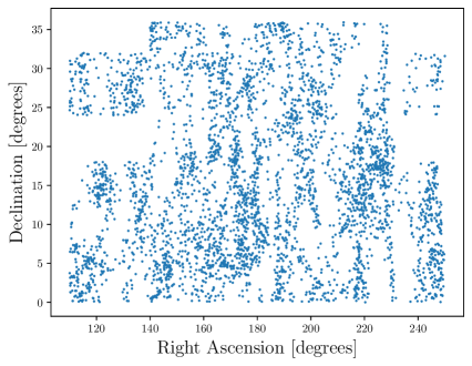
Figure 6: Footprint of a mock realisation.

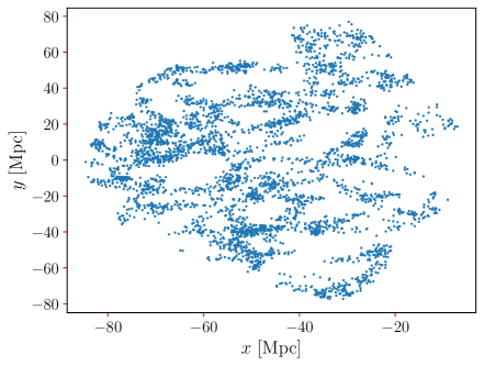
Figure 7: Cartesian projection of a mock realisation.

Ultimately, the most important feature needed in these mocks catalogues is that the 2-point correlation function of the Cox realisations reproduces at the scales of interest the correlation function obtained with the HI sample data. As a matter of fact, in figure 8, we show the difference between the Cox realisations (i.e., the mock catalogues) and the HI sample data. Each curve indicates the difference $\xi^{\text{Cox}}_{i}(r)-\xi^{\text{HI}}(r)$, where $i$ varies from 1 to 1000. As we can see, there is an excellent agreement for scales above 2 Mpc. This inaccuracy at small scales can be seen in the covariance matrix, calculated as

$$\text{Cov}(X,Y)=\frac{1}{N}\sum_{i=1}^{N}(X_{i}-\bar{X})(Y_{i}-\bar{Y})\,,$$ (2)

where $N$ is the sample size, and $X$ and $Y$ represent the correlation values at different bins (i.e., different distances between pairs). In figure 9, we show the reduced covariance matrix.

Figure 8: Difference between the Cox realisations and the data correlation functions, $\xi_{Cox}(r)-\xi(r)$. Each line corresponds to one realisation; we plotted 1000 realisations. We expect the difference to be approximately equal to zero, which occurs on scales above 2 Mpc, due to the difficulties to adjust all scales involved in the Cox process.

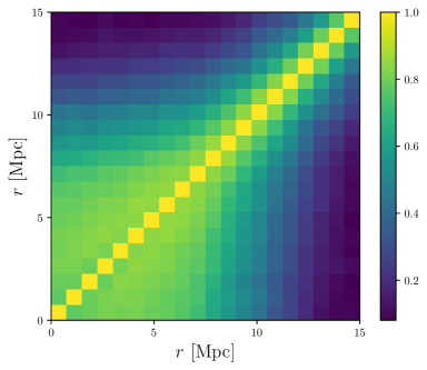
Figure 9: Reduced covariance (or correlation) matrix, $\text{Cov}(X,Y)/(\sigma(X)\sigma(Y))$, obtained from equation (2) and with $\sigma(X)$, $\sigma(Y)$ being the standard deviations of $X$ and $Y$.

In order to measure the uncertainties for the 2-point correlation function obtained using the ALFALFA data, we calculate the two-dimensional covariance matrix $\text{Cov}(X,Y)$ for the correlation function given in (11). Note that there is a high correlation on small scales, which decreases as we increase the scale. Therefore, by using the covariance matrix in our analyses, we are taking into account for the error evaluation important to quantify systematic effects of the selected sample, such as the sky surveyed area, depth of the survey, numerical density of cosmic objects, etc.

Consequently, the covariance matrix $\text{Cov}(X,Y)$ provides a more robust measure of the relationships between observational variables, highlighting significant correlations and quantifying the influence of individual variances. In fact, this tool helps to identify possible correlation patterns, and is particularly useful in our study because we are interested in the analyses across different scale distances.

3 Theoretical frame and Methodology

The standard cosmological model describes the mass distribution through the power spectrum of matter density fluctuations, as a function of scale. This function helps to describe the evolution of matter clustering and to understand the problem of structure formation, at several scales. In this section, we explore fundamental concepts to measure the matter fluctuations in the ALFALFA data.

3.1 Matter fluctuations

The physical processes of matter clustering and structure formation began in the early universe from primordial density fluctuations (Peebles, 1967; Feldman et al., 1994; Padmanabhan, 1993; Mo et al., 2010). The evolution of these fluctuations is conveniently studied through a dimensionless quantity, the density contrast $\delta(\mathbf{r},t)\equiv[\rho(\mathbf{r},t)-\rho_{0}(t)]/\rho_{0}(t)$, where the linear perturbation theory, for structure formation, follows whenever $\delta(\mathbf{r},t)\ll 1$.

Let’s study the density contrast at a given time in the early universe, $\delta(\mathbf{r})=\delta(\mathbf{r},t_{i})$, and assume that at different spatial locations $\delta(\mathbf{r})$ is very weakly correlated, i.e., it is a random variable (Padmanabhan, 1993). From this, one finds that its Fourier transform, $\delta_{\mathbf{k}}$, is Gaussian, therefore $\delta_{\mathbf{k}}$ is completely specified by its two moments: zero mean $\langle\delta_{\mathbf{k}}\rangle=0$, and variance $\sigma_{k}^{2}\equiv\langle|\delta_{\mathbf{k}}|^{2}\rangle$, where $\sigma_{k}^{2}$ is the power spectrum of the density fluctuations, commonly termed $P(k)$. The power spectrum, $P(k)$, is the Fourier transform of the two-point correlation function, $\xi(r)$, which is a primary estimator of the large-scale matter distribution

$$P(k)=\int\xi(r)e^{-i\mathbf{k}\cdot\mathbf{r}}\,d^{3}r\,.$$ (3)

A way to describe the clustering strength of a given ensemble of cosmic objects is to calculate the variance of the number counts within randomly placed spheres of a given radius $R$, which, considering the linear perturbations, can be written as

$$\sigma^{2}(R)=\frac{1}{2\pi^{2}}\int P(k)\,W_{R}^{2}(k)\,k^{2}\,dk\,,$$ (4)

where $W_{R}$ is the top-hat window with spherical symmetry (Mo et al., 2010). The variance of galaxy distribution is used to normalize (3). The function $\sigma^{2}(R)$ can be understood in terms of the variation in mass in a set of randomly placed windows, then one can show that the mass variance is (Mo et al., 2010)

$$\sigma^{2}_{M}(R)=\left\langle\left(\frac{\Delta M}{M_{0}}\right)^{2}\right\rangle_{\!\textbf{x}}\equiv\sigma^{2}(R)\,,$$ (5)

where $\Delta M\equiv M(\textbf{x},R)-M_{0}(R)$, $M(\textbf{x},R)$ is the mass in a window centered at x, and $M_{0}(R)$ is the average of the mass defined at the scale $R$. It is also possible to write $\sigma^{2}(R)$ as

$$\sigma^{2}(R)=\int\limits_{0}^{R^{-1}}\frac{dk}{k}\Delta_{k}^{2}\,,$$ (6)

where $\Delta_{k}^{2}$ is a dimensionless quantity proportional to the power spectrum and which expresses the contribution to the variance by the power in a unit logarithmic interval of $k$ (Padmanabhan, 1993)

$$\Delta_{k}^{2}\equiv\frac{k^{3}}{2\pi^{2}}P(k)\,.$$ (7)

It is useful to define the following quantity, which is related to $\xi(r)$ by (Padmanabhan, 1993)

$$J_{3}(R)\equiv\int_{0}^{R}r^{2}\xi(r)dr\,,$$ (8)

where this function gives us information about the spatial distribution of objects, because it represents weighted average of correlation function across different scales. Another way to represent $J_{3}(R)$ is

$$J_{3}(R)\simeq\frac{R^{3}}{3}\int\limits_{0}^{R^{-1}}\frac{dk}{k}\Delta_{k}^{2}\,,$$ (9)

where we note that combining equations (6) and (9) we obtain

$$\sigma^{2}(R)=\frac{3J_{3}(R)}{R^{3}}\,,$$ (10)

therefore, knowing $J_{3}(R)$ it is possible to calculate the mass variance at the scale $R$, i.e., $\sigma^{2}(R)$. Finally, one defines $\sigma_{8}\equiv\sigma(R=8\,h^{-1}\,\text{Mpc})$, at the scale $R=8\,h^{-1}$ Mpc.

3.2 Correlation function

We have previously seen in the section 3.1 that it is possible to relate the 2-point correlation function with the matter variance on different scales through equations (8) and (10). Therefore, we shall apply the 2-point correlation function $\xi(r)$ to the ALFALFA catalogue to calculate the matter variance. The most widely used correlation function estimator is the Landy-Szalay (Landy & Szalay, 1993), that returns the smallest discrepancies for a given cumulative probability, has no bias and nearly Poisson variance (Kerscher et al., 2000). This estimator is given by

$$\xi(r)\equiv\frac{DD(r)-2DR(r)+RR(r)}{RR(r)}\,,$$ (11)

where $DD(r)$ is the number of pairs in the sample data with distance separation $r$, normalized by the total number of pairs; $RR(r)$ is a similar quantity, but for the pairs in a random sample; and $DR(r)$ corresponds to a cross-correlation between a data object and a random object. Using $\xi(r)$ it is possible to determine the excess probability of finding two points from a dataset at a given distance separation $r$ when compared to a random distribution. In practice, to obtain $\xi(r)$ we use the TreeCorr code (Jarvis et al., 2004) .

3.2.1 Power-law approximation

The expectation regarding the 2-point correlation function is that it behaves according to a power-law (Peebles, 1993; Papastergis et al., 2013), that is,

$$\xi(r)=\left(\frac{r}{r_{0}}\right)^{-\gamma}\,,$$ (12)

where $r_{0}$ is a scale parameter that determines the characteristic scale of the correlation, and the parameter $\gamma$ quantifies the clustering of the cosmic tracer in study.

3.2.2 Constraining Power Law Parameters Using Bayesian Inference

In order to determine the optimal power law parameters, $r_{0}$ and $\gamma$, from the correlation function measurements, we adopt a Bayesian analysis approach (for more details, see e.g.,Verde (2010); Hobson et al. (2014); Trotta (2017)). This involves exploring the parameter space using the Markov Chain Monte Carlo (MCMC) algorithm implemented through the publicly available emcee code (Goodman & Weare, 2010; Foreman-Mackey et al., 2013).

In Bayesian analysis, our aim is to determine the probability of a given model with parameters $\bm{\theta}$ given a set of observations $\bm{D}$. This involves computing the posterior probability distribution $P(\bm{\theta}|\bm{D})$, which is given by

$$P(\bm{\theta}|\bm{D})=\frac{P(\bm{D}|\bm{\theta})P(\bm{\theta})}{P(\bm{D})}\,,$$ (13)

where $P(\bm{D}|\bm{\theta})$ is the likelihood function, $P(\bm{\theta})$ is the prior distribution, and $P(\bm{D})$ is the evidence. As $P(\bm{D})$ can be treated like a normalisation, we can look only for the scaled posterior. The logarithm of the scaled posterior distribution can be expressed as

$$\log P(\bm{\theta}|\bm{D})\propto\log P(\bm{D}|\bm{\theta})+\log P(\bm{\theta})\,,$$ (14)

where the likelihood can be written as

$$\log P(\bm{D}|\bm{\theta})\propto-\frac{1}{2}\chi^{2}\,.$$ (15)

In this work,

$$\chi^{2}=\sum_{i,j}\left[\xi(r_{i})-\xi^{\text{PL}}(r_{i};r_{0},\gamma)\right]\times C_{i,j}^{-1}(r_{i},r_{j})\times\left[\xi(r_{j})-\xi^{\text{PL}}(r_{j};r_{0},\gamma)\right]\,,$$ (16)

where $\xi(r_{i})$ represents the measured correlation function, $\xi^{\text{PL}}(r_{i};r_{0},\gamma)$ is the model prediction with power law parameters $r_{0}$ and $\gamma$, and $C_{i,j}^{-1}(r_{i},r_{j})$ is the inverse covariance matrix of the measurements, given by equation (2).

In retrospect, looking at the work of (Martin et al., 2012), we have properly selected the space parameter prior, as indicated in table 1.

Parameter	Range	Initial Guess
$r_{0}$	$1~{}\text{Mpc}<r_{0}<15~{}\text{Mpc}$	5.0 Mpc
$\gamma$	$1<\gamma<3$	1.8

Table 1: Prior ranges and initial guesses for the power-law parameters.

4 Results and Discussion

Applying the statistical tools outlined in section 3, we analysed the selected sample described in section 2. Firstly, we calculated the 2-point correlation function, $\xi(r)$, for our data sample for pair distances in the interval $[0.5,15]\,\text{Mpc}$; our result can be seen in figure 10, where we consider $20$ bins. Similarly, we applied the same procedure to a set of $1000$ mock catalogues generated from the Cox process, as detailed in section 2.3, to estimate the covariance matrix using equation (2) and subsequently determine the uncertainties associated with our results. The findings are illustrated in figure 10.

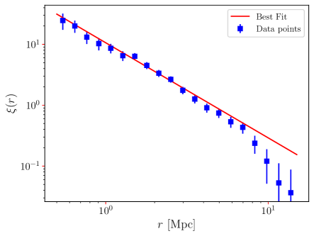
Figure 10: 2-point correlation function for the HI sample in study using, 1000 realisations of the Cox process to estimate the uncertainties. For the best fit it was assumed the power-law relationship, equation (12).

The best fit curve was plotted considering the power-law shown in equation (12), where the fitting parameters $r_{0}=4.5\pm 0.3\,\text{Mpc}$ and $\gamma=1.55\pm 0.07$ were obtained using the MCMC method (cf. section 3.2.2 and figure 11). The data agree well with the expected power-law function up to $r\simeq 7\,\text{Mpc}$. Beyond this scale, the observed decline in the data with respect to the best fit, is indicative of a limited sample volume, and the power-law correlation function does not suitably describe the distribution of matter structures (Martin et al., 2012).

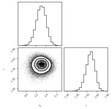
Figure 11: Joint and marginal distributions of the power-law parameters $r_{0}$ and $\gamma$.

To deepen our analysis, we calculated the $\sigma(R)$ values. By using the $\xi(r)$ values and the previously obtained covariance matrix, we can get the mass fluctuation function, which is shown in figure 12. The data points were obtained directly from the square root of equation (10) leading to a direct measurement of the matter fluctuation of the HI extragalactic sources, $\sigma_{8}^{\text{tr}}=\sigma_{8}^{\text{HI}}=0.92\pm 0.05$ at scales $r=8$ Mpc. The red curve corresponds to the theoretical model for the matter fluctuations assuming the Planck’s flat-$\Lambda$CDM model. The dashed gray line is the best-fit expectation for $\sigma(R)$ when one assumes the power-law to for the 2-point correlation function, for this we call this dashed gray line as $\sigma$-model. We observe a good agreement, at $2\sigma$ level, between the $\sigma$-model and the data. As noticed above the 2-point correlation function does not follow a power-law for scales above 7 Mpc, in consequence, this fact is translated to the $\sigma(R)$ computation, and manifests increasing the discrepancy between $\sigma$-model and data, as observed in figure 12. For both the $\sigma$-model and the data, there is a transition with respect to the $\Lambda$CDM model around 4 Mpc, suggestive of a possible transition between non-linear to linear scales. As the scale increases, both $\sigma$-model and data fall below the $\Lambda$CDM model, consistently, indicating that the HI sources are anti-biased with respect to the underlying matter fluctuation field (Basilakos et al., 2007).

The scale where our best-fit data intersects the $\Lambda$CDM model, which results from a linear theory, is suggestive of the transition between the non-linear and linear regimes. We find, however, that a more appropriate scale would be to consider the scale where the matter fluctuation is $\sigma(R)=1$, because such scale would be a model-independent quantity in data analyses where distances scales are in Mpc units (and not $h^{-1}$ Mpc). When we apply this condition to our best-fit analysis (see figure 12) we obtain $R=7.2\pm 1.5~{}\text{Mpc}$. This could be considered as the transition scale where the linear relationship is valid $\delta_{\text{HI}}=b_{\text{HI}}\delta_{M}$, i.e., the fluctuation of matter of the HI sources is proportional to the fluctuation of underlying matter.

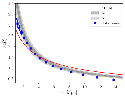
Figure 12: Mass fluctuation for the selected HI sample from ALFALFA. The best fit was assumed to follow a power-law, equation (12). The shaded gray areas correspond to $1\sigma$ and $2\sigma$ confidence levels. Note that there is an intersection between the data best-fit and the theoretical model $\Lambda$CDM, suggestive of a transition between non-linear and linear scales in the behaviour of $\sigma(R)$. Beyond this scale, the matter fluctuation of the HI sample consistently falls below the $\Lambda$CDM prediction, implying an anti-bias in our sample relative to the underlying matter.

To determine $\sigma_{8}$ from our measurement, $\sigma_{8}^{\text{HI}}$, it is essential to assume a value for the linear bias, $b_{\text{HI}}$. This linear bias, in turn, requires assuming a normalisation, $\sigma_{8}$, for the power spectrum when performing statistical analyses that compares models and observations (Basilakos et al., 2007). In summary, our $\sigma_{8}$ measurement serves as a consistency test for the $\Lambda$CDM model. However, within our approach we can study the effect of the Hubble constant on our $\sigma_{8}$ measurement, since one must assume a value of $h$ in order to transform the Mpc units to $h^{-1}~{}\text{Mpc}$ units.

Considering the linear bias for the HI extragalactic sources obtained by Obuljen et al. (2019), $b_{\text{HI}}=0.875\pm 0.022$, and using the relation

$$\sigma_{8}=\frac{\sigma_{8}^{\text{HI}}}{b_{\text{\,HI}}}\,,$$ (17)

with uncertainties given by

$$\delta\sigma_{8}=\frac{\sigma_{8}^{\text{HI}}}{b_{\text{\,HI}}}\sqrt{\left(\frac{\delta\sigma_{8}^{\text{HI}}}{\sigma_{8}^{\text{HI}}}\right)^{2}+\left(\frac{\delta b_{\text{\,HI}}}{b_{\text{\,HI}}}\right)^{2}}\,,$$ (18)

we conclude that $\sigma_{8}=1.05\pm 0.06$ at the scale of $8$ Mpc. Furthermore, we consider a set of values for the Hubble parameter: $h=\{0.6727,\,0.698,\,0.7304\}$ to determine the $\sigma(R)$ at the scale $R=8h^{-1}\,\text{Mpc}$ in each case. The results, with their respective uncertainties, taking into account the bias are listed in table 2.

	$h$	$\sigma_{8}^{\text{HI}}$	$\sigma_{8}$
	$0.6727$ (Planck Collaboration et al., 2020)	$0.68\pm 0.04$	$0.78\pm 0.04$
	$0.698$ (Freedman, 2021)	$0.70\pm 0.04$	$0.80\pm 0.05$
	$0.7304~{}\text{\cite[citep]{(\@@bibref{AuthorsPhrase1Year}{Riess22}{\@@citephrase{, }}{})}}$	$0.73\pm 0.04$	$0.83\pm 0.05$

Table 2: Our measurements of $\sigma_{8}^{\text{HI}}$ and $\sigma_{8}$ at the scale $8\,h^{-1}\,\text{Mpc}$ considering diverse measurements of $h$.

As can be seen in the plots of the probability density functions shown in figure 13 and in the $H_{0}-\sigma_{8}$ parameter space in figure 14, considering the tension metric between two estimates $A$ and $B$,

$$T_{\sigma_{8}}=\frac{|\sigma_{8,A}-\sigma_{8,B}|}{\sqrt{\sigma_{\sigma_{8},A}+\sigma_{\sigma_{8},B}}}\,,$$ (19)

we find that our measurements of $\sigma_{8}$ agrees at $0.79\,\sigma$ and $0.36\,\sigma$ confidence levels with Planck Planck Collaboration et al. (2020) and ACT Madhavacheril et al. (2024) results, respectively.

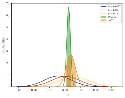
Figure 13: Probability distribution function of $\sigma_{8}$ for different values of the Hubble parameter $h$.

Despite $\Lambda\text{CDM}$ model best fits observational data, it still faces significant challenges, such as the tensions arising from measurements of the Hubble constant, $H_{0}$ and $\sigma_{8}$. Within the $\Lambda\text{CDM}$ framework, measurements using CMB data yield $H_{0}=67.27\pm 0.60$ km s^-1 Mpc^-1 (Planck Collaboration et al., 2020), whereas local measurements using Type Ia supernovae obtain $H_{0}=73.04\pm 1.04$ km s^-1 Mpc^-1 (Riess et al., 2022), indicating a discrepancy of $\sim 5\sigma$ between direct and indirect measurements (Perivolaropoulos & Skara, 2022; Di Valentino et al., 2021a, c; Verde et al., 2023; Tully et al., 2023). Regarding $\sigma_{8}$, Planck Collaboration et al. (2020) reports a value of $\sigma_{8}=0.8120\pm 0.0073$, which is corroborated by Madhavacheril et al. (2024), where $\sigma_{8}=0.819\pm 0.015$, but they both disagree with direct measurements, such as weak lensing, RSD, and galaxy clustering in $\sim 3\sigma$ (Perivolaropoulos & Skara, 2022; Adhikari et al., 2022; Di Valentino et al., 2021b).

The search for alleviating these tensions motivated numerous recent studies, which report values of $\sigma_{8}\sim 0.75$ (Freedman, 2021; Tröster et al., 2020; Nunes & Vagnozzi, 2021; Heymans et al., 2021). As illustrated in figure 14, each value of $h$ provides a distinct value of $\sigma_{8}$ in units of $h^{-1}$ Mpc. Our $\sigma_{8}$ measurement obtained through the ALFALFA data agrees at $0.79\,\sigma$ with the value reported in Planck Collaboration et al. (2020), using for this comparison the $h$ value provided by the Planck Collaboration. Similarly, when adopting the value calculated by Freedman (2021), $h=0.698$, we remain $0.36\,\sigma$ away from the value reported by Madhavacheril et al. (2024). Some authors suggest that, despite the $\sigma_{8}$ tension potentially arising from systematic errors (in either CMB or LSS evaluation) or sample variance (originated from different regions observed by different surveys), it may indicate the necessity for a new physics beyond the standard model to explain the tension in $\sigma_{8}$ and $H_{0}$ (Nunes & Vagnozzi, 2021; Adhikari et al., 2022; Perivolaropoulos & Skara, 2022; Amon & Efstathiou, 2022; Schöneberg et al., 2022; Poulin et al., 2023; Abdalla et al., 2022). Nevertheless, we can safely conclude that, considering the data pairs $(\sigma_{8},H_{0})$ from the Planck CMB and ACT CMB-lensing analyses, our $\sigma_{8}$ measurement agrees with them in less than $1\,\sigma$ confidence level.

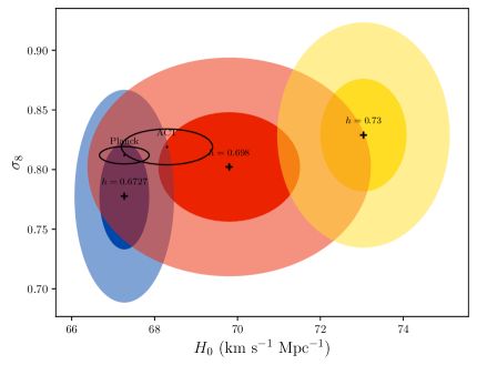
Figure 14: $H_{0}-\sigma_{8}$ parameter space for different values of $h$. The probability ellipses show $1\sigma$ and $2\sigma$ CL. We compare our results with the ACT and Planck data.

5 Conclusions

The search for the cosmological model that describes the observed universe on large scales motivate the use of astronomical data to explore alternative models through diverse approaches (de Carvalho et al., 2020; Krishnan et al., 2022; Luongo et al., 2022; Giarè et al., 2024; Giarè, 2024; Dinda & Banerjee, 2024; Dinda, 2024; Ribeiro et al., 2024; Oliveira et al., 2023). In this scenario, the measurement of the galaxies density fluctuation in the universe is a crucial feature for understanding its large-scale structure, turning the determination of the $\sigma_{8}$ parameter an important task in modern cosmology. It is estimated that this fluctuation in the Local Universe is approximately 1 on scales of $8\,h^{-1}$ Mpc (Juszkiewicz et al., 2010). Over the years, various research teams have come together to measure the matter fluctuations using diverse techniques and cosmic tracers (Hasselfield et al., 2013; Reid et al., 2010; Melchiorri et al., 2003; Hamana et al., 2003), seeking a better understanding of the tendency for galaxies to cluster more densely than the underlying dark matter and the amplitude of primordial fluctuations in the universe, resulting from physical processes during its early stages. The amplitude of mass fluctuations describes the normalization of the linear spectrum of mass fluctuations in the early universe, as described in section 3.1, the spectrum that seeded galaxy formation. The abundance of massive clusters depends exponentially on this parameter (Bahcall & Bode, 2003), because a high amplitude of mass fluctuations forms structures rapidly in the early times, while a lower amplitude forms structures more slowly.

The increasing tension surrounding the value of $\sigma_{8}$ necessitates additional studies and analyses with varied datasets and different methodologies to obtain a more precise and comprehensive understanding of matter fluctuation amplitudes in the universe. In our work, we analyzed the large-scale structure of the universe using data from the ALFALFA extragalactic HI survey. Our focus was on characterizing matter fluctuations and understanding mass variance on different spatial scales, utilizing the HI extragalactic sources as tracers of the underlying matter distribution.

We investigated the matter fluctuation $\sigma(R)$ by applying the 2-point correlation function to a selected sample of the ALFALFA survey, and using the relation between this quantity and $J_{3}(R)$. The derived value of $\sigma_{8}^{\text{HI}}=0.92\pm 0.05$ aligns with the expectations for galaxy distribution and is consistent with the prediction of the $\Lambda\text{CDM}$ model for a sample with bias factor $b<1$. When we consider the bias for HI sources, $b_{\text{HI}}$, this yields $\sigma_{8}=1.05\pm 0.06$. Considering different values for the Hubble parameter, we found that each value of $h$ provides a distinct value of $\sigma_{8}$, which is different from the previous measurements from Planck and ACT at $0.79\sigma$ and $0.36\sigma$, respectively.

Our results obtained from the analyses of the ALFALFA data highlight the robustness of our methodology to measure the matter fluctuations in the Local Universe, potentially contributing to the ongoing discussion concerning the $\sigma_{8}$, or $S_{8}$, tension.

Data Availability

The data underlying this article will be shared on reasonable request to the corresponding author.

Appendix A Robustness test with curve fitting

For robustness, in this appendix, we also conducted a Curve Fitting of the data for the theoretical function (12), using the scipy.optimize package from the Open Source library in Python language, where we performed the best-fit analysis of the parameters $\gamma$ and $r_{0}$, in order that they minimize the $\chi^{2}$ function defined in equation (16), where Cov^-1 is the inverse of the covariance matrix, and Cov is specified in equation (2). The uncertainties of the adjusted parameters, $\{\sigma_{i}\}$, are given by the square roots of the diagonal elements of the covariance matrix, $\sigma_{i}=\sqrt{\text{Cov}_{ii}}$.

In figure 15, the fit is shown the best fit curve, where we obtain $r_{0}=4.5\pm 0.4\text{; and}\,\gamma=1.56\pm 0.11$. As observed in table 3, the adjusted parameters values are the same as those obtained using the MCMC method, with an increase anticipated in error bars, which is expected due to the difference in the methods employed.

	$r_{0}$ [Mpc]	$\gamma$
MCMC	$4.5\pm 0.3$	$1.55\pm 0.07$
Curve Fitting	$4.5\pm 0.4$	$1.56\pm 0.11$

Table 3: The adjusted parameters using MCMC and Curve Fitting methods.

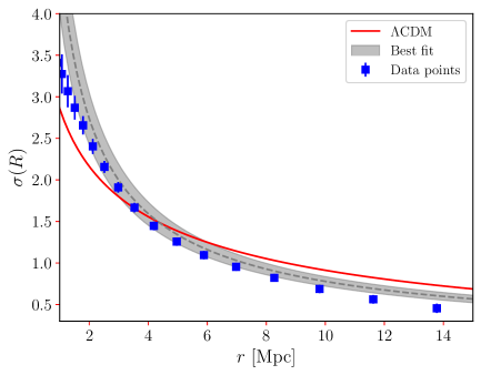
Figure 15: The mass fluctuation analysis for the HI sample using the Curve Fitting method.

Appendix B The impact of the Virgo cluster as a non-linear effect

Our $\sigma_{8}$ measurement was obtained for an ensemble of cosmic objects with distances in the interval $20-85$ Mpc, a purposeful choice to avoid the overdense spatial region, where $\delta>1$, containing the Virgo cluster. In this Appendix we study the impact of the presence of the Virgo cluster in our measurement. For this, we analyze the HI objects with distances in the interval $10-85$ Mpc, which includes the Virgo cluster. At the same time, considering for this test those cosmic objects that are closer to us we are also increasing a systematic effect sourced by large peculiar velocities (Avila et al., 2023; Lopes et al., 2024; Kalbouneh et al., 2023; Migkas et al., 2021).

We perform this consistency analysis recalculating the $\sigma(R)$ function. Our result is shown in figure 16, where for comparison we also plot the original case. As expected, some differences can be observed, being the difference more noticeable at the smaller scales where the clustering, that is, the value of $\sigma(R)$, is bigger, presumably due to the presence of more clustered structures like Virgo.

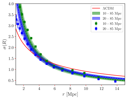
Figure 16: Comparison between two ALFALFA samples with HI sources belonging to distinct distance intervals. The green points corresponds to the sample with sources in the interval $10-85~{}\text{Mpc}$; the blue points corresponds to sources in the interval $20-85~{}\text{Mpc}$. The shaded areas correspond to $1\sigma$ and $2\sigma$ confidence levels for each sample.

Nevertheless, in both cases $\sigma(R)$ agrees at the $2\sigma$ level, confirming the robustness of our measurement.

References

- Abdalla et al. (2022) Abdalla E., et al., 2022, Journal of High Energy Astrophysics, 34, 49
- Adhikari et al. (2022) Adhikari R. X., et al., 2022, arXiv e-prints, p. arXiv:2209.11726
- Amon & Efstathiou (2022) Amon A., Efstathiou G., 2022, mnras, 516, 5355
- Avila et al. (2018) Avila F., Novaes C. P., Bernui A., de Carvalho E., 2018, jcap, 2018, 041
- Avila et al. (2019) Avila F., Novaes C. P., Bernui A., de Carvalho E., Nogueira-Cavalcante J. P., 2019, mnras, 488, 1481
- Avila et al. (2021) Avila F., Bernui A., de Carvalho E., Novaes C. P., 2021, mnras, 505, 3404
- Avila et al. (2022) Avila F., Bernui A., Bonilla A., Nunes R. C., 2022, European Physical Journal C, 82, 594
- Avila et al. (2023) Avila F., Oliveira J., Dias M. L. S., Bernui A., 2023, Brazilian Journal of Physics, 53, 49
- Avila et al. (2024) Avila F., de Carvalho E., Bernui A., Lima H., Nunes R. C., 2024, mnras, 529, 4980
- Bahcall & Bode (2003) Bahcall N. A., Bode P., 2003, apjl, 588, L1
- Basilakos et al. (2007) Basilakos S., Plionis M., Kovač K., Voglis N., 2007, mnras, 378, 301
- Borgani et al. (1995) Borgani S., Plionis M., Coles P., Moscardini L., 1995, mnras, 277, 1191
- Di Valentino et al. (2021a) Di Valentino E., et al., 2021a, Classical and Quantum Gravity, 38, 153001
- Di Valentino et al. (2021b) Di Valentino E., et al., 2021b, Astroparticle Physics, 131, 102604
- Di Valentino et al. (2021c) Di Valentino E., et al., 2021c, Astroparticle Physics, 131, 102605
- Dinda (2024) Dinda B. R., 2024, European Physical Journal C, 84, 402
- Dinda & Banerjee (2024) Dinda B. R., Banerjee N., 2024, arXiv e-prints, p. arXiv:2403.14223
- Efstathiou (1995) Efstathiou G., 1995, mnras, 276, 1425
- Efstathiou et al. (1990) Efstathiou G., Kaiser N., Saunders W., Lawrence A., Rowan-Robinson M., Ellis R. S., Frenk C. S., 1990, mnras, 247, 10P
- Feldman et al. (1994) Feldman H. A., Kaiser N., Peacock J. A., 1994, apj, 426, 23
- Foreman-Mackey et al. (2013) Foreman-Mackey D., Hogg D. W., Lang D., Goodman J., 2013, pasp, 125, 306
- Franco et al. (2024) Franco C., Avila F., Bernui A., 2024, mnras, 527, 7400
- Freedman (2021) Freedman W. L., 2021, apj, 919, 16
- Giarè (2024) Giarè W., 2024, arXiv e-prints, p. arXiv:2404.12779
- Giarè et al. (2024) Giarè W., Gómez-Valent A., Di Valentino E., van de Bruck C., 2024, prd, 109, 063516
- Goodman & Weare (2010) Goodman J., Weare J., 2010, Communications in Applied Mathematics and Computational Science, 5, 65
- Hamana et al. (2003) Hamana T., et al., 2003, apj, 597, 98
- Hasselfield et al. (2013) Hasselfield M., Hilton M., Marriage T. A., Addison G. E., Barrientos E. J., 2013, jcap, 2013, 008
- Haynes et al. (2018) Haynes M. P., et al., 2018, apj, 861, 49
- Heymans et al. (2021) Heymans C., et al., 2021, aap, 646, A140
- Hobson et al. (2014) Hobson M. P., Jaffe A. H., Liddle A. R., Mukherjee P., Parkinson D., 2014, Bayesian Methods in Cosmology. Cambridge University Press
- Jarvis et al. (2004) Jarvis M., Bernstein G., Jain B., 2004, mnras, 352, 338
- Juszkiewicz et al. (2010) Juszkiewicz R., Feldman H. A., Fry J. N., Jaffe A. H., 2010, jcap, 2010, 021
- Kaiser (1988) Kaiser N., 1988, mnras, 231, 149
- Kalbouneh et al. (2023) Kalbouneh B., Marinoni C., Bel J., 2023, prd, 107, 023507
- Keihänen et al. (2019) Keihänen E., et al., 2019, aap, 631, A73
- Kerscher et al. (2000) Kerscher M., Szapudi I., Szalay A. S., 2000, apjl, 535, L13
- Krishnan et al. (2022) Krishnan C., Mohayaee R., Colgáin E. Ó., Sheikh-Jabbari M. M., Yin L., 2022, prd, 105, 063514
- Landy & Szalay (1993) Landy S. D., Szalay A. S., 1993, apj, 412, 64
- Lopes et al. (2024) Lopes M., Bernui A., Franco C., Avila F., 2024, apj, 967, 47
- Luongo et al. (2022) Luongo O., Muccino M., Colgáin E. Ó., Sheikh-Jabbari M. M., Yin L., 2022, prd, 105, 103510
- Madhavacheril et al. (2024) Madhavacheril M. S., et al., 2024, apj, 962, 113
- Martin et al. (2012) Martin A. M., Giovanelli R., Haynes M. P., Guzzo L., 2012, apj, 750, 38
- Martinez & Saar (2001) Martinez V. J., Saar E., 2001, Statistics of the galaxy distribution. Chapman and Hall/CRC
- Martinez et al. (1998) Martinez V. J., Pons-Borderia M.-J., Moyeed R. A., Graham M. J., 1998, mnras, 298, 1212
- Masters (2005) Masters K. L., 2005, PhD thesis, Cornell University, New York
- Melchiorri et al. (2003) Melchiorri A., Bode P., Bahcall N. A., Silk J., 2003, apjl, 586, L1
- Migkas et al. (2021) Migkas K., Pacaud F., Schellenberger G., Erler J., Nguyen-Dang N. T., Reiprich T. H., Ramos-Ceja M. E., Lovisari L., 2021, aap, 649, A151
- Mo et al. (2010) Mo H., Van den Bosch F., White S., 2010, Galaxy formation and evolution. Cambridge University Press
- Norberg et al. (2009) Norberg P., Baugh C. M., Gaztañaga E., Croton D. J., 2009, mnras, 396, 19
- Nunes & Vagnozzi (2021) Nunes R. C., Vagnozzi S., 2021, mnras, 505, 5427
- Obuljen et al. (2019) Obuljen A., Alonso D., Villaescusa-Navarro F., Yoon I., Jones M., 2019, mnras, 486, 5124
- Oliveira et al. (2023) Oliveira F., Avila F., Bernui A., Bonilla A., Nunes R. C., 2023, arXiv e-prints, p. arXiv:2311.14216
- Padmanabhan (1993) Padmanabhan T., 1993, Structure formation in the universe. Cambridge university press
- Pandey (2010) Pandey B., 2010, mnras, 401, 2687
- Papastergis et al. (2013) Papastergis E., Giovanelli R., Haynes M. P., Rodríguez-Puebla A., Jones M. G., 2013, apj, 776, 43
- Peebles (1967) Peebles P. J. E., 1967, apj, 147, 859
- Peebles (1993) Peebles P. J. E., 1993, Principles of Physical Cosmology. Princeton University Press, doi:10.1515/9780691206721
- Perivolaropoulos & Skara (2022) Perivolaropoulos L., Skara F., 2022, nar, 95, 101659