Theory Driven Evolution of the Weak Mixing Angle

Abstract

We present the first purely theoretical calculation of the weak mixing angle in the $\overline{\mathrm{MS}}$ scheme at low energies by combining results from lattice QCD with perturbation theory. We discuss its correlation with the hadronic contribution to the anomalous magnetic moment of the muon and to the energy dependence of the electromagnetic coupling. We also compare the results with calculations using cross-section data as input. Implications for the Standard Model prediction of the mass of the $W$ boson are also discussed.

The weak mixing angle, $\theta_{W}$, is a central parameter in the Standard Model (SM) of particle physics, featuring prominently in many precision observables, such as parity violation, neutrino physics, or $Z$-pole measurements. Thus, it serves as a useful tool for studying the consistency of the SM across different energy scales. In particular, the upcoming low-energy parity violating electron scattering experiments P2 at Mainz Becker et al. (2018) and MOLLER Benesch et al. (2014) at JLab profit from an enhanced sensitivity due to an accidental suppression of the left-right polarization cross section asymmetries which are proportional to $1-4\sin^{2}\theta_{W}\ll 1$. Just as the predecessor experiments SLAC–E158 Anthony et al. (2005) and JLab–Qweak Androić et al. (2018) they are sensitive to higher-order SM corrections Czarnecki and Marciano (1996, 2000), especially from the $\gamma Z$ vacuum polarization function. The level of precision at P2 and MOLLER requires even the inclusion of two-loop electroweak effects Du et al. (2021); Erler et al. (2022).

Analogous to the dependence on the energy scale $\mu$ of the electromagnetic coupling, $\hat{\alpha}(\mu)$, i.e., its running, higher order terms, in particular $\gamma Z$ vacuum polarization effects, can be incorporated into the running of the weak mixing angle. The large logarithms that emerge when using the weak mixing angle measured at high energy colliders as input in low-energy processes, call for a systematic inclusion and re-summation of higher order corrections. This procedure is renormalization scheme dependent. For computational simplicity we choose the $\overline{\mathrm{MS}}$ scheme (denoted by a caret), where $\hat{\theta}_{W}$ is defined in terms of the SM gauge couplings $\hat{g}$ and $\hat{g}^{\prime}$,

$$\hat{s}^{2}\equiv\sin^{2}\hat{\theta}_{W}=\frac{\hat{g}^{\prime 2}}{\hat{g}^{2}+\hat{g}^{\prime 2}}\ .$$ (1)

Ref. Erler and Ramsey-Musolf (2005) derived a relation between $\hat{\theta}_{W}(\mu)$ and $\hat{\alpha}(\mu)$ in the $\overline{\mathrm{MS}}$ scheme (see Ref. Jegerlehner (1986) for an approach using a different scheme). This allowed to straightforwardly include non-perturbative hadronic contributions to the running of $\hat{\theta}_{W}$ by using $e^{+}e^{-}$ annihilation data in a dispersion relation. The main source of uncertainty was due to the necessary flavor separation, defined as the contribution of the strange quark current relative to the up and down quark currents. Significant progress was reported in Ref. Erler and Ferro-Hernández (2018) where improved data, a more precise flavor separation estimate, and the inclusion of higher-order perturbative QCD (pQCD) corrections, led to a noticeable reduction in the total uncertainty in $\hat{s}^{2}(0)$.

In a different development, there is a discrepancy between the measured Bennett et al. (2006); Abi et al. (2021); Aguillard et al. (2023) and predicted Aoyama et al. (2020); Keshavarzi et al. (2020); Davier et al. (2020); Jegerlehner (2020) values of the anomalous magnetic moment of the muon, $a_{\mu}$ (employing $e^{+}e^{-}$ data for the hadronic vacuum polarization contribution $a^{\mathrm{hvp}}_{\mu}$). Recently, the results of the CMD-3 experiment Ignatov et al. (2023) revealed further tension when compared with $e^{+}e^{-}$ data sets from previous experiments. Moreover, ab-initio lattice QCD (LQCD) calculations Giusti et al. (2019); Shintani and Kuramashi (2019); Davies et al. (2020); Gérardin et al. (2019); Borsanyi et al. (2021); Aubin et al. (2022) are in reasonable agreement with the measured $a_{\mu}$ and CMD-3. Since $e^{+}e^{-}$ data also enter into calculations of $\hat{\alpha}$ and $\hat{\theta}_{W}$, these tensions should affect these quantities as well, and an effort is required to incorporate LQCD results in the respective SM predictions. A first step in this direction Erler and Ferro-Hernandez (2023) showed how LQCD can be used in an optimal way to include hadronic effects into the running of $\hat{\alpha}$. A parametric expression in terms of input parameters was given, simplifying the implementation into global electroweak (EW) fits.

Applying the framework of Refs. Erler and Ramsey-Musolf (2005); Erler and Ferro-Hernández (2018); Erler and Ferro-Hernandez (2023), and obtaining the flavor separation entirely from LQCD, we derive a purely theoretical SM prediction of $\hat{s}^{2}(0)$ in terms of $\hat{s}^{2}(M_{Z})$, where $M_{Z}$ is the mass of the $Z$ boson. We also give a simplified formula which can be included into EW fitting libraries. Finally, we quantify the correlations between $\hat{s}^{2}(0),\hat{\alpha}(M_{Z})$, and $a^{\mathrm{hvp}}_{\mu}$.

We find a discrepancy between the lattice and the data-driven predictions for the running. This tension (which induces a positive shift of $\sim 8\times 10^{-5}$ in $\hat{s}^{2}(0)$ when experimental data are replaced by LQCD), is about 30% of the uncertainty anticipated for future low-energy parity-violating experiments. On the other hand, if this issue can be resolved, we would be left with a residual uncertainty of $\delta\hat{s}^{2}(0)=2\times 10^{-5}$, negligible for the low-energy parity-violating experiments in the foreseeable future.

Our starting point is the vacuum polarization function,

$$\hat{\Pi}(q^{2},\mu^{2})=-\frac{i}{3q^{2}}\int d^{4}xe^{iqx}\langle 0|TJ^{\mu}(x)J_{\,\mu}(0)|0\rangle$$ (2)

where $J^{\mu}$ is the electromagnetic current. LQCD computes the subtracted vacuum polarization function, $\Pi(-Q^{2})=\hat{\Pi}(0,\mu^{2})-\hat{\Pi}(-Q^{2},\mu^{2})$. For large enough $Q^{2}$, pQCD can be used to obtain the subtraction constant $\hat{\Pi}(0,\mu^{2})$ which encodes the running of the $\overline{\mathrm{MS}}$ couplings. Indeed, setting $Q^{2}=\mu^{2}$, we arrive at the result in the $\overline{\mathrm{MS}}$ scheme by adding

$$\hat{\Pi}(-Q^{2},Q^{2})=\sum_{f}\frac{Q^{2}_{f}}{4\pi^{2}}\sum^{3}_{n=0}c_{n}\frac{\hat{\alpha}_{s}^{n}(Q^{2})}{\pi^{n}},$$ (3)

to the lattice results. Here, $\hat{\alpha}_{s}$ is the strong coupling, and the constants,

$$c_{0} =\frac{5}{3}-6\frac{\hat{m}^{2}_{f}}{Q^{2}}\ , c_{1} =-0.22489-16\ \frac{\hat{m}^{2}_{f}}{Q^{2}}\ ,$$

$$c_{2} =0.8522-144.85\ \frac{\hat{m}^{2}_{f}}{Q^{2}}\ , c_{3} =5.588\ ,$$

where $\hat{m}_{f}$ is the $\overline{\mathrm{MS}}$ mass of fermion $f$ at the scale $Q$, were obtained with the help of Refs. Nesterenko (2016); Maier and Marquard (2012); Chetyrkin et al. (1996, 2000); Shifman et al. (1979); Eidelman et al. (1999); Surguladze and Tkachov (1990); Braaten et al. (1992). We use this conversion formula only at energy scales where the three light quarks can be treated as approximately degenerate, so that the disconnected piece vanishes.

The running of $\hat{\alpha}$ is given by

$$\hat{\alpha}(\mu)=\frac{\alpha}{1-\Delta\hat{\alpha}(\mu)}\ ,$$ (4)

where $\Delta\hat{\alpha}(\mu)=4\pi\alpha\hat{\Pi}(0,\mu^{2})$ and $\alpha\approx 1/137.036$. In a first step and with the help of Eqs. (3) and (4), we compute $\hat{\alpha}(\mu)$ at some reference scale $\mu$ somewhat above the hadronic region employing LQCD from the Mainz collaboration Cè et al. (2022). Then, we use the renormalization group equation (RGE) which is known up to order $\hat{\alpha}^{4}_{s}$ Baikov et al. (2012) to compute $\hat{\alpha}(M_{Z})$. At the threshold of each particle, the matching conditions given in Refs. Chetyrkin et al. (1998); Sturm (2014) are applied. Thus, dependence on $\hat{\alpha}_{s}$ and the heavy quark masses, $\hat{m}_{c}$, and $\hat{m}_{b}$, is induced.

parameter	result $\times 10^{4}$	correlations
$\Pi_{\mathrm{disc}}$	.$-3.8\pm 0.2$	1.0	0.8	0.8
$\Pi_{s}$	$\phantom{0}83.0\pm 1.4$	0.8	1.0	0.96
$\Pi_{ud}$	$587.8\pm 8.3$	0.8	0.96	1.0

Table 1: Values, errors, and correlations for the vacuum polarization function at $Q^{2}=4\mbox{ GeV}^{2}$. They were obtained from Appendix F of Ref. Cè et al. (2022) assuming that the disconnected contribution is associated with the $u$ and $d$ quarks. The isospin error was assigned entirely to the up and down contribution.

Since the running of $\hat{\theta}_{W}$ is related to that of $\hat{\alpha}$ through the photon vector polarization function, we can relate the solutions to their RGEs Erler and Ramsey-Musolf (2005); Erler and Ferro-Hernández (2018), and in the process re-sum the logarithms in $\hat{s}^{2}(\mu)$,

$$\hat{s}^{2}(\mu)=\hat{s}^{2}(\mu_{0})\frac{\hat{\alpha}(\mu)}{\hat{\alpha}(\mu_{0})}+\lambda_{1}\left[1-\frac{\hat{\alpha}(\mu)}{\hat{\alpha}(\mu_{0})}\right]+$$

$$\frac{\hat{\alpha}(\mu)}{\pi}\left[\frac{\lambda_{2}}{3}\ln\frac{\mu^{2}}{\mu_{0}^{2}}+\frac{3\lambda_{3}}{4}\ln\frac{\hat{\alpha}(\mu)}{\hat{\alpha}(\mu_{0})}+\tilde{\sigma}(\mu_{0})-\tilde{\sigma}(\mu)\right]\ .$$ (5)

The $\lambda_{i}$ are constants, and the quantities $\tilde{\sigma}$ contain the contributions from disconnected diagrams. Both depend on the number of active particles $n_{f}$, so that $\hat{s}^{2}(\mu)$ is a piecewise function in which the number of particle types change when a threshold is crossed and the matching conditions Erler and Ramsey-Musolf (2005); Erler and Ferro-Hernández (2018) are used. With $\hat{\alpha}(\mu)$ known at the reference scale $\mu$, we use Eq. (5) and the matching conditions to compute $\hat{s}^{2}(\mu)$ in terms of $\hat{s}^{2}(M_{Z})$.

However, the aforementioned dependence of Eq. (5) on $n_{f}$ requires separate information regarding the relative contributions of strange versus up and down quarks (flavor separation) in the hadronic (non-perturbative) region, as well as from disconnected diagrams. To address this, we translate the results by the Mainz lattice collaboration Cè et al. (2022), which are given in terms of the $SU(3)$ labeled vacuum polarization functions, $\Pi_{33}$, $\Pi_{88}$, and $\Pi_{08}$, into the connected pieces $\Pi_{\mathrm{ud}}$ and $\Pi_{s}$, as well as the disconnected piece $\Pi_{\mathrm{disc}}$. This is shown in Tab. 1 together with the associated correlation matrix which we computed by assuming that each lattice error induced by a given source (like scale setting, model error or statistical) enters fully correlated. Finally, we use Eq. (3) to convert these results to the $\overline{\mathrm{MS}}$ scheme, and with the flavor separation at hand we can apply Eq. (5).

source	$\delta\sin^{2}\hat{\theta}_{W}(0)\times 10^{5}$
LQCD	2.3
pQCD	0.1
condensates	0.2
total	2.3

Table 2: Uncertainties in the calculation of the low energy weak mixing angle.

We computed $\hat{s}^{2}(0)$ numerically, displaying explicitly the dependence on $\hat{s}^{2}(M_{Z})$, $\hat{\alpha}_{s}$, $\hat{m}_{c}$, $\hat{m}_{b}$, the LQCD input, as well as the strange quark and gluon condensates. We write our main result as $\hat{s}^{2}(0)=\hat{\kappa}(0)\hat{s}^{2}(M_{Z})$, with

$$\hat{\kappa}(0) =1.03234-0.43\,\Delta\hat{s}^{2}_{Z}+0.030\,\Delta\hat{\alpha}_{s}$$

$$-0.0012\,\Delta\hat{m}_{c}-0.0003\,\Delta\hat{m}_{b}$$

$$-0.111\,\Delta\Pi_{\mathrm{disc}}+0.206\,\Delta\Pi_{s}+0.087\,\Delta\Pi_{ud}$$

$$+\frac{0.003}{\mathrm{GeV}^{4}}\,\langle m_{s}\bar{s}s\rangle+\frac{0.0004}{\mathrm{GeV}^{4}}\,\left\langle\frac{\hat{\alpha}_{s}}{\pi}G^{2}\right\rangle\ ,$$ (6)

where we defined,

$$\Delta\hat{s}^{2}_{Z} \equiv\hat{s}^{2}(M_{Z})-0.23122\ ,$$

$$\Delta\hat{\alpha}_{s} \equiv\hat{\alpha}_{s}(M_{Z})-0.1185\ ,$$

$$\Delta\hat{m}_{c} \equiv\hat{m}_{c}(\hat{m}_{c})-1.274\mbox{ GeV}\ ,$$

$$\Delta\hat{m}_{b} \equiv\hat{m}_{b}(\hat{m}_{b})-4.180\mbox{ GeV}\ .$$ (7)

$\Delta\Pi_{X}$ is the difference between $\Pi_{X}$ ($X=\mathrm{disc},s$, or $ud$) at $Q^{2}=4\mbox{ GeV}^{2}$ and the central value shown in Tab. 1.

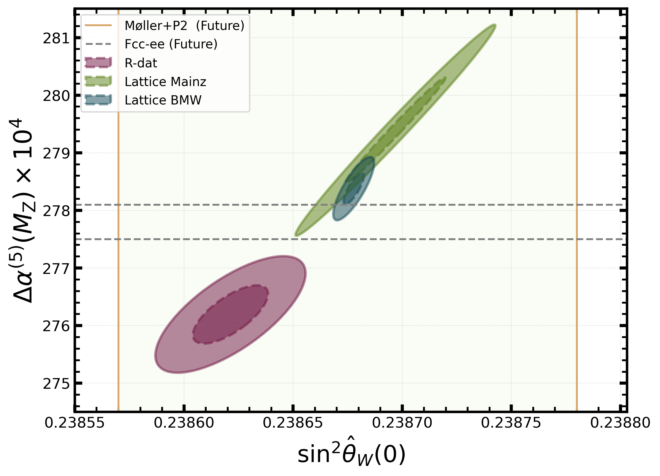
Figure 1: $\Delta\chi^{2}=1$ and $\Delta\chi^{2}=4$ contours for $\sin^{2}\hat{\theta}_{W}(0)$ and $\Delta\alpha^{(5)}(M_{Z})$. The yellow region represents the expected combined 1 $\sigma$ band for P2 and MOLLER. The horizontal grey dashed band shows a projection Blondel and Janot (2022) for the FCC-ee. Only low energy (data and lattice) and pQCD errors are included.

Eq. (6) shows that the LQCD uncertainty amounts to $1.0\times 10^{-4}$ in $\hat{\kappa}(0)$ and the perturbative uncertainty, conservatively taken to correspond to the last known terms in the RGE (of order $\hat{\alpha}^{4}_{s}$), the decoupling relations, and the scheme conversion in Eq. (3), is $4\times 10^{-6}$. The uncertainty from the condensates amount to $1\times 10^{-5}$ (taking a conservative 100% error of $0.003\mbox{ GeV}^{4}$ in the strange quark condensate McNeile et al. (2013) and of $0.01\,\mathrm{GeV}^{4}$ in the gluon condensate Narison (2012); Dominguez et al. (2015)). The corresponding error budget for $\hat{s}^{2}(0)$ is shown in Tab. 2. The linearized result (6) approximates the exact numerical solution to better than 1 ppm even for values $3~{}\sigma$ away from the reference values.

One can compare these results to those that use $e^{+}e^{-}\rightarrow\mathrm{hadrons}$ cross section data as input. There, large terms proportional to powers of $\pi^{2}$ are introduced when passing from timelike to spacelike momenta, enhancing the pQCD contribution and uncertainty. Furthermore, the result from the data driven approach, $\hat{\kappa}(0)_{e^{+}e^{-}}=1.03201\pm 0.00008$ Erler and Ferro-Hernández (2018), differs from Eq. (6) by $0.00033$ or about $3~{}\sigma$. This is another reflection of the tension between LQCD and cross section data observed in the context of $\hat{\alpha}$ and $a_{\mu}$.

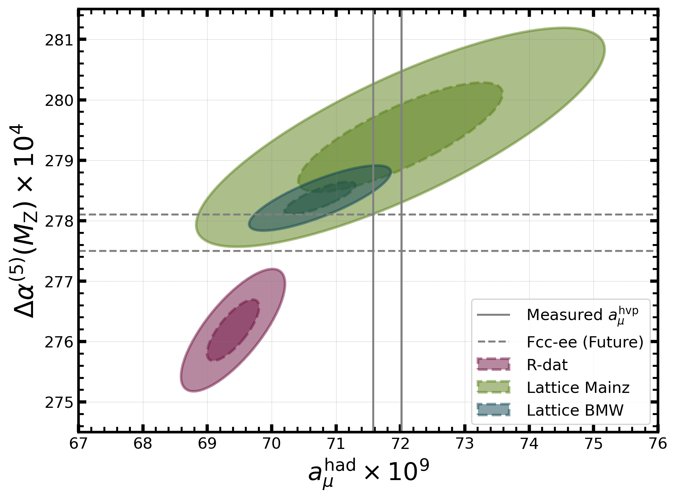
Figure 2: $\Delta\chi^{2}=1$ and $\Delta\chi^{2}=4$ contours for $\Delta\alpha^{(5)}(M_{Z})$ and $a^{\mathrm{hvp}}_{\mu}$ (cf. Fig. 1). The width of the vertical band corresponds to the current experimental uncertainty in $a_{\mu}$.

As shown in Fig. 1, $\hat{s}^{2}(0)$ and $\hat{\alpha}$ are correlated. Three input cases are considered for illustration, namely from LQCD Cè et al. (2022), from $e^{+}e^{-}$ data Davier et al. (2020) and from the lattice BMW collaboration Borsanyi et al. (2018), where we assumed the same correlation between flavors as at Mainz.

We also show the $1~{}\sigma$ bands projected for the future parity violation measurements Becker et al. (2018); Benesch et al. (2014) (vertical yellow band) and the FCC-ee Blondel and Janot (2022) (horizontal dashed grey line). In order not to dilute the tension between LQCD and data, the dependence on $\hat{\alpha}_{s}$ and the $\hat{m}_{q}$ is ignored in all figures. A larger correlation is seen when LQCD results are used, as unlike in the data driven approach the flavor separation uncertainty entering in $\hat{s}^{2}(0)$ is correlated with the uncertainty in the sum of all flavors.

Investigating this kind of theoretical correlation is particularly important for EW global fits in the ultra-precision era. Thus, the correlations of $\Delta\alpha^{(5)}(M_{Z})$ and $\hat{s}^{2}(0)$ with $a^{\mathrm{hvp}}_{\mu}$ need to be evaluated and implemented, as well. Since the calculation of $a^{\mathrm{hvp}}_{\mu}$ involves a momentum integral, knowledge of the $Q^{2}$ dependence of the vacuum polarization function is needed including uncertainties and point-by-point correlations. To estimate these from Ref. Cè et al. (2022) we computed the statistical correlation for a subset of ensembles, and assumed the systematic errors as $100\%$ correlated. We find a Pearson correlation coefficient of 0.8 between $a^{\mathrm{hvp}}_{\mu}$ and $\Delta\alpha^{(5)}(M^{2}_{Z})$. The various error sources enter with $Q^{2}$-dependent weights that breaks the otherwise nearly perfect correlation between the two quantities. On the other hand, the assumed correlation within each source of uncertainty is much less significant, as even taking the systematic errors to be uncorrelated reduces the correlation merely by a few percent. As for the case of cross section data, Refs. Davier et al. (2024); Malaescu and Schott (2021) estimate the correlation between $a^{\mathrm{hvp}}_{\mu}$ and the low energy contribution ($<2$ GeV) to $\Delta\alpha^{(5)}(M_{Z})$ to $0.8$, as well. We show these results in Fig. 2.

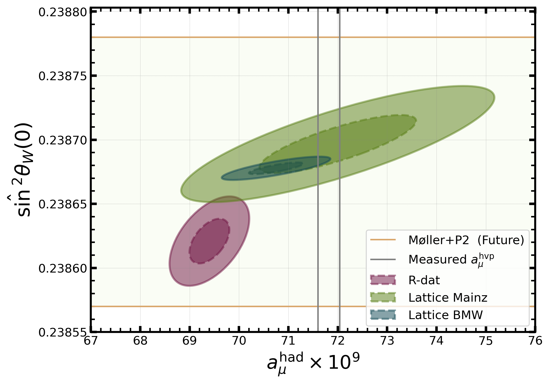
Figure 3: $\Delta\chi^{2}=1$ and $\Delta\chi^{2}=4$ contours for $\hat{s}^{2}(0)$ and $a^{\mathrm{hvp}}_{\mu}$ (cf. Figs. 1) and 2).

Finally, the calculation of the correlation between $\hat{s}^{2}(0)$ and $a^{\mathrm{hvp}}_{\mu}$ from LQCD requires the point-by-point correlation of each flavor separately. However, since the dominant errors are very similar for the $\gamma Z$ and $\gamma\gamma$ vacuum polarization functions at $\mu\approx 2$ GeV, one can expect the correlation of $a^{\mathrm{hvp}}_{\mu}$ with $\hat{s}^{2}(0)$ to be about the same as the one with $\Delta\alpha^{(5)}(M_{Z})$. The result is shown in Fig. 3.

In summary, if one uses either the Mainz LQCD result Cè et al. (2022) or else cross section data as input into EW global fits, the values given in the upper or lower panel of Tab. 3 apply, respectively. The parameter dependencies from Eq. (7) and the condensates are not included, but can easily be added by using Eq. (6); for the data driven approach the corresponding dependencies can be found in Refs. Erler and Ferro-Hernandez (2023); Erler and Ferro-Hernández (2018).

parameter	result	correlations
$\hat{\kappa}(0)-1$	$(323.4\pm 1.0)\times 10^{-4}$	1.0	0.98	0.9
$\Delta\alpha^{(5)}(M_{Z})$	$(279.4\pm 0.9)\times 10^{-4}$	0.98	1.0	0.8
$a^{\mathrm{hvp}}_{\mu}$	$(72.0\pm 1.6)\times 10^{-9}$	0.8	0.8	1.0
$\hat{\kappa}(0)-1$	$(320.1\pm 0.8)\times 10^{-4}$	1.0	0.7	0.5
$\Delta\alpha^{(5)}(M_{Z})$	$(276.2\pm 0.5)\times 10^{-4}$	0.7	1.0	0.8
$a^{\mathrm{hvp}}_{\mu}$	$(69.4\pm 0.4)\times 10^{-9}$	0.5	0.8	1.0

Table 3: Values, errors, and correlations for the running of $\sin^{2}\hat{\theta}_{W}$, of the hadronic contribution to $\hat{\alpha}(M_{Z})$, and to $a_{\mu}$ when the input is provided by LQCD Cè et al. (2022) (upper panel) and by $e^{+}e^{-}$ data Davier et al. (2020) (lower panel).

Constraints on $\Delta\alpha^{(5)}(M_{Z})$ are important for the SM prediction of the mass $M_{W}$ of the $W$ boson. Inserting the values et al (2024) $m_{t}=172.85$ GeV and $M_{Z}=91.1884$ GeV together with the Higgs boson mass, $M_{H}=125.10$ GeV and the central values of the heavy quark masses and the strong coupling constant in Eq. (7) into the numerical formula obtained in Refs. Freitas et al. (2002); Awramik et al. (2004), we can compute $M_{W}$ from a given value of $\Delta\alpha^{(5)}(M_{Z})$. The results are shown in Tab. 4 together with the experimental world average Amoroso et al. (2024), which excludes the recent discrepant result by the CDF Collaboration at the Tevatron Aaltonen et al. (2022).

Using the correlations obtained here, we can compute the shifts in the predictions of $M_{W}$, when $a^{\mathrm{hvp}}_{\mu}$ is adjusted such that the SM prediction of $a_{\mu}$ in Ref. Aoyama et al. (2020) would coincide with the experimental value Aguillard et al. (2023). In the case of the data driven approach, $a^{\mathrm{hvp}}_{\mu}$ would shift by 6 times its uncertainty, which for a correlation of 0.8 implies that $\Delta\alpha^{(5)}(M_{Z})$ has to increase by $2\times 10^{-4}$. This translates into a decrease in the SM prediction of $M_{W}$ by 4 MeV. On the other hand, given the good agreement of LQCD with the current experimental value, the change is only 0.2 MeV and 0.8 MeV for the results Cè et al. (2022) and Borsanyi et al. (2018), respectively. A complete investigation of the impact of LQCD on EW global fits is left for future work.

In this letter we introduced a procedure for the systematic implementation of the hadronic vacuum polarization obtained from lattice QCD to $\hat{s}^{2}(0)$ and other high-precision EW observables. We used the RGE to re-sum higher order logarithms entering the calculation of $\hat{s}^{2}(0)$, and presented a parametric formula for a straightforward implementation in global EW fits. Furthermore, we compared this result with the one obtained from cross section data, and found a tension which is consistent with the known one in $\Delta\alpha^{(5)}(M_{Z})$. Finally, we quantified the correlation of $\hat{s}^{2}(0)$ with $\Delta\alpha^{(5)}(M_{Z})$ and $a^{\mathrm{hvp}}_{\mu}$. As an example for the implications of the strong positive correlations that we found on other EW observables we estimated the effects on the SM prediction of the $W$ boson mass.

We hope this work will help to better connect Lattice QCD with more traditional approaches to electroweak precision physics. For example, we suggest to provide the results for several $Q^{2}$ in a flavor-separated way, including correlations. A future direction will address the correlations introduced by the results on the strong coupling constant from LQCD.

source	$M_{W}$ [GeV]
$e^{+}e^{-}$ data	$80.3575\pm 0.0009$
LQCD (Mainz)	$80.3516\pm 0.0017$
LQCD (BMW)	$80.3535\pm 0.0005$
experiment (excluding CDF)	$80.3692\pm 0.0133$

Table 4: Predictions for $M_{W}$ using the results of Ref. Freitas et al. (2002). The shown errors correspond to the nonparametric ones in $\Delta\alpha^{(5)}$. The last line is the experimental measurement obtained from the combination in Ref. Amoroso et al. (2024).

References

- Becker et al. (2018) D. Becker et al., Eur. Phys. J. A 54, 208 (2018).
- Benesch et al. (2014) J. Benesch et al. (MOLLER), The MOLLER Experiment: An Ultra-Precise Measurement of the Weak Mixing Angle Using Møller Scattering (2014), eprint 1411.4088.
- Anthony et al. (2005) P. L. Anthony et al. (SLAC E158), Phys. Rev. Lett. 95, 081601 (2005).
- Androić et al. (2018) D. Androić et al. (Qweak), Nature 557, 207 (2018).
- Czarnecki and Marciano (1996) A. Czarnecki and W. J. Marciano, Phys. Rev. D 53, 1066 (1996).
- Czarnecki and Marciano (2000) A. Czarnecki and W. J. Marciano, Int. J. Mod. Phys. A 15, 2365 (2000).
- Du et al. (2021) Y. Du, A. Freitas, H. H. Patel, and M. J. Ramsey-Musolf, Phys. Rev. Lett. 126, 131801 (2021).
- Erler et al. (2022) J. Erler, R. Ferro-Hernández, and A. Freitas, JHEP 08 (2022).
- Erler and Ramsey-Musolf (2005) J. Erler and M. J. Ramsey-Musolf, Phys. Rev. D 72, 073003 (2005).
- Jegerlehner (1986) F. Jegerlehner, Z. Phys. C 32, 195 (1986).
- Erler and Ferro-Hernández (2018) J. Erler and R. Ferro-Hernández, JHEP 03, 196 (2018).
- Bennett et al. (2006) G. W. Bennett et al. (Muon g-2), Phys. Rev. D 73, 072003 (2006).
- Abi et al. (2021) B. Abi et al. (Muon g-2), Phys. Rev. Lett. 126, 141801 (2021), eprint 2104.03281.
- Aguillard et al. (2023) D. P. Aguillard et al. (Muon g-2), Phys. Rev. Lett. 131, 161802 (2023).
- Aoyama et al. (2020) T. Aoyama et al., Phys. Rept. 887, 1 (2020).
- Keshavarzi et al. (2020) A. Keshavarzi, D. Nomura, and T. Teubner, Phys. Rev. D 101, 014029 (2020).
- Davier et al. (2020) M. Davier, A. Hoecker, B. Malaescu, and Z. Zhang, Eur. Phys. J. C 80, 241 (2020), [Erratum: Eur.Phys.J.C 80, 410 (2020)].
- Jegerlehner (2020) F. Jegerlehner, CERN Yellow Reports: Monographs 3, 9 (2020).
- Ignatov et al. (2023) F. V. Ignatov et al. (CMD-3), Measurement of the cross section from threshold to 1.2 GeV with the CMD-3 detector (2023), eprint 2302.08834.
- Giusti et al. (2019) D. Giusti et al., Phys. Rev. D 99, 114502 (2019).
- Shintani and Kuramashi (2019) E. Shintani and Y. Kuramashi (PACS), Phys. Rev. D 100, 034517 (2019).
- Davies et al. (2020) C. T. H. Davies et al. (MILC), Phys. Rev. D 101, 034512 (2020).
- Gérardin et al. (2019) A. Gérardin et al., Phys. Rev. D 100, 014510 (2019).
- Borsanyi et al. (2021) S. Borsanyi et al., Nature 593, 51 (2021).
- Aubin et al. (2022) C. Aubin, T. Blum, M. Golterman, and S. Peris, Phys. Rev. D 106, 054503 (2022).
- Erler and Ferro-Hernandez (2023) J. Erler and R. Ferro-Hernandez, JHEP 12, 131 (2023).
- Nesterenko (2016) A. V. Nesterenko, Strong interactions in spacelike and timelike domains: dispersive approach (Elsevier, 2016).
- Maier and Marquard (2012) A. Maier and P. Marquard, Nucl. Phys. B 859, 1 (2012).
- Chetyrkin et al. (1996) K. G. Chetyrkin, J. H. Kuhn, and M. Steinhauser, Nucl. Phys. B 482, 213 (1996).
- Chetyrkin et al. (2000) K. G. Chetyrkin, R. V. Harlander, and J. H. Kuhn, Nucl. Phys. B 586, 56 (2000), [Erratum: Nucl.Phys.B 634, 413–414 (2002)].
- Shifman et al. (1979) M. A. Shifman, A. I. Vainshtein, and V. I. Zakharov, Nucl. Phys. B 147, 385 (1979).
- Eidelman et al. (1999) S. Eidelman, F. Jegerlehner, A. L. Kataev, and O. Veretin, Phys. Lett. B 454, 369 (1999).
- Surguladze and Tkachov (1990) L. R. Surguladze and F. V. Tkachov, Nucl. Phys. B 331, 35 (1990).
- Braaten et al. (1992) E. Braaten, S. Narison, and A. Pich, Nucl. Phys. B 373, 581 (1992).
- Cè et al. (2022) M. Cè et al., JHEP 08, 220 (2022).
- Baikov et al. (2012) P. A. Baikov, K. G. Chetyrkin, J. H. Kuhn, and J. Rittinger, JHEP 07, 017 (2012).
- Erler (1999) J. Erler, Phys. Rev. D 59, 054008 (1999).
- Chetyrkin et al. (1998) K. G. Chetyrkin, B. A. Kniehl, and M. Steinhauser, Nucl. Phys. B 510, 61 (1998).
- Sturm (2014) C. Sturm, Eur. Phys. J. C 74, 2978 (2014).
- Davier et al. (2023) M. Davier et al., JHEP 04, 067 (2023).
- Hernández (2023) R. F. Hernández, AdlerPy: A Python Package for the Perturbative Adler Function (2023), eprint 2311.04849.
- Blondel and Janot (2022) A. Blondel and P. Janot, Eur. Phys. J. Plus 137, 92 (2022).
- McNeile et al. (2013) C. McNeile et al., Phys. Rev. D 87, 034503 (2013).
- Narison (2012) S. Narison, Phys. Lett. B 706, 412 (2012).
- Dominguez et al. (2015) C. A. Dominguez, L. A. Hernandez, K. Schilcher, and H. Spiesberger, JHEP 03, 053 (2015).
- Borsanyi et al. (2018) S. Borsanyi et al. (BMW), Phys. Rev. Lett. 121, 022002 (2018).
- Davier et al. (2024) M. Davier, Z. Fodor, A. Gerardin, L. Lellouch, B. Malaescu, F. M. Stokes, K. K. Szabo, B. C. Toth, L. Varnhorst, and Z. Zhang, Phys. Rev. D 109, 076019 (2024), eprint 2308.04221.
- Malaescu and Schott (2021) B. Malaescu and M. Schott, Eur. Phys. J. C 81, 46 (2021).
- et al (2024) S. N. et al (Particle Data Group), Phys. Rev. D 110, 030001 (2024).
- Freitas et al. (2002) A. Freitas, W. Hollik, W. Walter, and G. Weiglein, Nucl. Phys. B 632, 189 (2002), [Erratum: Nucl.Phys.B 666, 305–307 (2003)].
- Awramik et al. (2004) M. Awramik, M. Czakon, A. Freitas, and G. Weiglein, Phys. Rev. D 69, 053006 (2004), eprint hep-ph/0311148.
- Amoroso et al. (2024) S. Amoroso et al. (LHC-TeV MW Working Group), Eur. Phys. J. C 84, 451 (2024).
- Aaltonen et al. (2022) T. Aaltonen et al. (CDF), Science 376, 170 (2022).