Coding schemes in neural networks learning classification tasks
Abstract
Neural networks posses the crucial ability to generate meaningful representations of task-dependent features. Indeed, with appropriate scaling, supervised learning in neural networks can result in strong, task-dependent feature learning. However, the nature of the emergent representations, which we call the ‘coding scheme’, is still unclear. To understand the emergent coding scheme, we investigate fully-connected, wide neural networks learning classification tasks using the Bayesian framework where learning shapes the posterior distribution of the network weights. Consistent with previous findings, our analysis of the feature learning regime (also known as ‘non-lazy’, ‘rich’, or ‘mean-field’ regime) shows that the networks acquire strong, data-dependent features. Surprisingly, the nature of the internal representations depends crucially on the neuronal nonlinearity. In linear networks, an analog coding scheme of the task emerges. Despite the strong representations, the mean predictor is identical to the lazy case. In nonlinear networks, spontaneous symmetry breaking leads to either redundant or sparse coding schemes. Our findings highlight how network properties such as scaling of weights and neuronal nonlinearity can profoundly influence the emergent representations.
I Introduction
The remarkable empirical success of deep learning stands in strong contrast to the theoretical understanding of trained neural networks. Although every single detail of a neural network is accessible and the task is known, it is still very much an open question how the neurons in the network manage to collaboratively solve the task. While deep learning provides exciting new perspectives on this problem, it is also at the heart of more than a century of research in neuroscience.
Two key aspects are representation learning and generalization. It is widely appreciated that neural networks are able to learn useful representations from training data [1, 2, 3]. But from a theoretical point of view, fundamental questions about representation learning remain wide open: Which features are extracted from the data? And how are those features represented by the neurons in the network? Furthermore, neural networks are able to generalize even if they are deeply in the overparameterized regime [4, 5, 6, 7, 8, 9] where the weight space contains a subspace—the solution space—within which the network perfectly fits the training data. This raises a fundamental question about the effect of implicit and explicit regularization: Which regularization biases the solution space towards weights that generalize well?
We here investigate the properties of the solution space using the Bayesian framework where the posterior distribution of the weights determines how the solution space is sampled [10, 11]. For theoretical investigations of this weight posterior, the size of the network is taken to infinity. Crucially, the scaling of the network and task parameters, as the network size is taken to infinity, has a profound impact: neural networks can operate in different regimes depending on this scaling. Here, the relevant scales are the width of the network and the size of the training data set . A widely used scaling limit is the infinite width limit where is taken to infinity while remains finite [12, 13, 14, 15, 16, 17, 18, 19]. A scaling limit closer to empirically trained networks takes both and to infinity at fixed ratio [20, 21, 22, 23, 24, 25, 26].
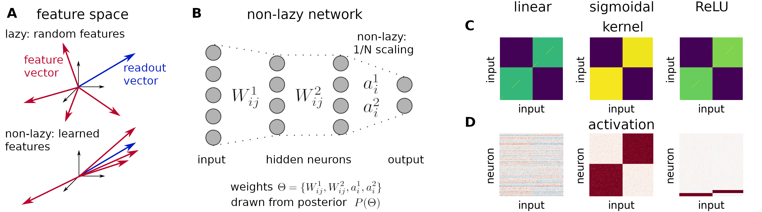
In addition to scaling of and , the scaling of of the final network output with is important because it has a strong effect on representation learning [27, 28, 29] (illustrated in Fig. 1A). If the readout scales its inputs with the network operates in the ‘lazy’ regime. Lazy networks rely predominantly on random features and representation learning is only a correction both for finite [30, 31, 32, 18, 33] and fixed [20]; in the latter case it nonetheless affects the predictor variance [20, 24, 25]. If the readout scales its inputs with the network operates in the ‘non-lazy’ (also called mean-field or rich) regime and learns strong, task-dependent representations [34, 35, 36, 37, 38, 39, 40] (illustrated in Fig. 1C). However, the nature of the solution, in particular how the learned features are represented by the neurons, remains unclear. Work based on a partial differential equations for the weights [34, 35, 36, 37] only provides insight in effectively low dimensional settings; investigations based on kernel methods [38, 39, 40] average out important structures at the single neuron level.
In this paper, we develop a theory for the weight posterior of non-lazy networks in the limit . We show that the representations in non-lazy networks trained for classification tasks exhibit a remarkable structure in the form of coding schemes, where distinct groups of neurons are characterized by the subset of classes that activate them. Another central result is that the nature of the learned representation strongly depends on the type of neuronal nonlinearity (illustrated in Fig. 1D). Owing to the influence of the nonlinearity, we consider three nonlinearities one after the other: linear, sigmoidal, and ReLU leading to analog, redundant, and sparse coding schemes, respectively. For each nonlinearity we first consider the learned representations on training inputs in the simple setting of a toy task and then investigate learned representations on training and test inputs and generalization on MNIST and CIFAR10. The paper concludes with a brief summary and discussion of our results.
II Results
II.1 Setup
We denote the output of a fully-connected feedforward networks with hidden layers and outputs (Fig. 1B) by
| (1) |
where denotes the neuronal nonlinearity, the last layer preactivation, and is an arbitrary -dimensional input. The preactivations are in the hidden layers and in the first layer. The activations are and we assume for simplicity that the width of all hidden layers is . Importantly, we scale the output with such that the network is in the non-lazy regime but the hidden layer preactivations with or (scaling with would instead corresponds to the lazy regime).
The trainable parameters of the networks are the readout and hidden weights, which we collectively denote by . The networks are trained using empirical training data containing inputs of dimension and targets of dimension . The matrix containing all training inputs is denoted by ; the matrix containing all training targets is denoted by .
II.1.1 Weight Posterior
The weight posterior is [20]
| (2) |
where is the partition function, a mean-squared error loss, and an i.i.d. zero-mean Gaussian prior with prior variances , for readout and hidden weights, respectively. Temperature controls the relative importance of the quadratic loss and the prior. In the overparameterized regime, the limit restricts the posterior to the solution space where the network interpolates the training data. For simplicity, we set in the main text. Throughout, we denote expectations w.r.t. the weight posterior by .
The interplay between loss and prior shapes the solutions found by the networks. Importantly, on the solution space the prior alone determines the posterior probability. Thus, the prior plays a central role for regularization which complements the implicit regularization due to the non-lazy scaling.
Scaling limit: We consider the limit while the number of readout units as well as the number of layers remain finite, i.e., . Because the gradient of is small due to the non-lazy scaling of the readout, the noise introduced by the temperature needs to be scaled down as well, requiring the scaling (see supplement). In the remainder of the manuscript denotes the rescaled temperature which therefore remains of as increases. In the present work, we focus on the regime where the training loss is essentially zero, and therefore consider the limit for the theory; to generate empirical samples from the weight posterior we use a small but non-vanishing rescaled temperature.
Under the posterior, the non-lazy scaling leads to large readout weights: the posterior norm per neuron grows with , thereby compensating for the non-lazy scaling. To avoid this undoing of the non-lazy scaling, we scale down with , guaranteeing that the posterior norm of the readout weights per neuron is . The precise scaling depends on the depth and the type of nonlinearity (see supplement).
In total there are three differences between (2) and the corresponding posterior in the lazy regime [20]: 1) The non-lazy scaling of the readout in (1) with instead of . 2) The scaling of the temperature with . 3) The prior variance of the readouts weights needs to be scaled down with .
Due to the symmetry of fully connected networks under permutations of the neurons, the statistics of the posterior weights must be invariant under permutations. However, for large and this symmetry may be broken at low so that the posterior consists of permutation broken branches which are disconnected from each other in weight space. A major finding of our work is the emergence of this spontaneous symmetry breaking and its far reaching consequences for the nature of the learned neural representations.
II.1.2 Kernel and Coding Schemes
Learned representations are frequently investigated using the kernel [e.g., 41, 42, 20, 39] which measures the overlap between the neurons’ activations on pairs of inputs:
| (3) |
where the inputs , can be either from the training or the test set. We denote the posterior averaged kernel by ; the posterior averaged kernel matrix on all training inputs is denoted by without arguments. In addition to capturing the learned representations, the kernel is a central observable because it determines the statistics of the output function in wide networks [12, 13, 14, 15].
Crucially, the kernels disregards how the learned features are represented by the neurons. Consider, for example, binary classification in two extreme cases: (1) each class activates a single neuron and all remaining neurons are inactive; (2) each class activates half of the neurons and the remaining half of the neurons are inactive. In both scenarios the kernels agree up to an overall scaling factor despite the drastic difference in the underlying representations (illustrated in Fig. 1(C,D)).
| Term | Definition |
|---|---|
| code | The subset of classes that activate a neuron. |
| coding scheme | The collection of codes implemented by a neuronal population. |
| sparse coding | Only a small subset of neurons exhibit codes. |
| redundant coding | All the codes in the scheme are shared by a large subset of neurons. |
| analog coding | All neurons respond to all classes but with different strength. |
The central goal of our work is to understand the nature of the representations. As illustrated above, this means that the theory needs to go beyond kernels. To this end, we use the notion of a neural code which we define as the subset of classes that activate a given neuron (see Table 1). At the population level, this leads to a “coding scheme”: the collection of codes implemented by the neurons in the population. As we will show the coding schemes encountered in our theory are of the three types (illustrated in Fig. 1(D)): 1) Sparse coding where only a small subset of neurons exhibit codes (as in the first scenario above). 2) Redundant coding where all the codes in the scheme are shared by a large subset of neurons (as in the second scenario above). 3) Analog coding where all neurons respond to all classes but with different strength.
As illustrated in Fig. 1(D), the nature of the learned representations varies crucially with the choice of the activation function of the hidden layer, , although the kernel matrix is similar in all cases. Specifically, in the linear case, , the coding is analog, in the sigmoidal case, , the coding is redundant, and in the case of ReLU, , the coding is sparse.
II.2 Linear Networks
To gain insight into the neural code and its relation to the nonlinearity we develop a mean field theory that is exact in the above scaling limit. We begin with linear networks because the theory is analytically solvable by adapting the techniques developed in [20] to non-lazy networks. In order to prevent growth of the norm of the readout weights with we set (see supplement). The theoretical results are in the zero temperature limit.
II.2.1 Training
We start with the learned representations on the training set. A key result of the theory is that the joint posterior of the readout weights and the activations factorizes across neurons and layers, , where denotes the -dimensional vector containing the readout weights for neuron and denotes the -dimensional vector containing the activations of neuron on all training inputs.
The single neuron readout posterior is Gaussian,
| (4) |
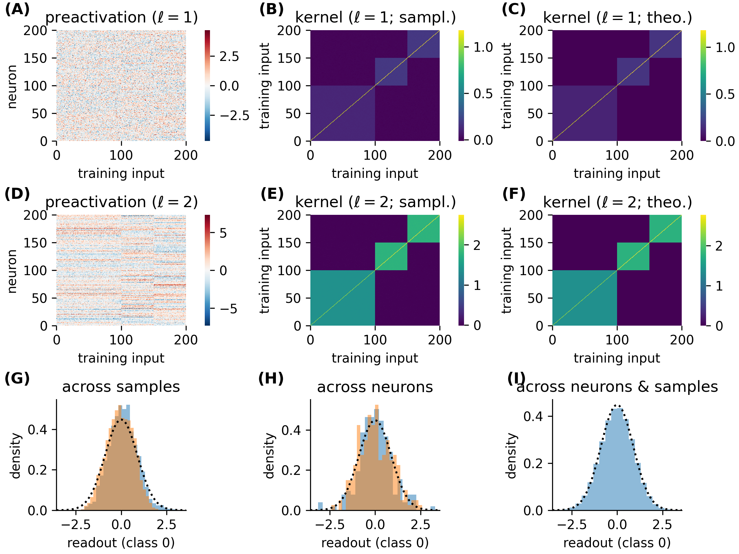
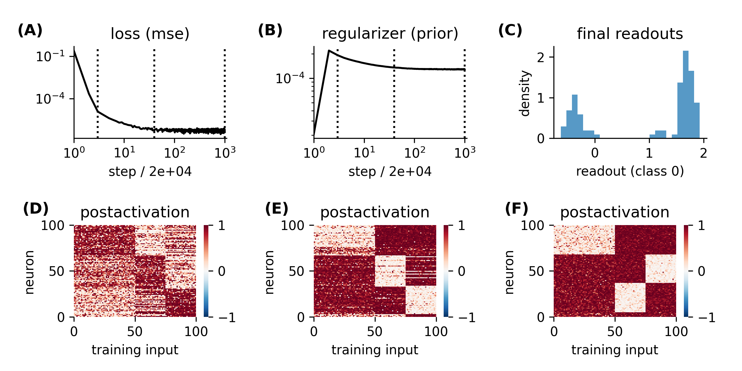
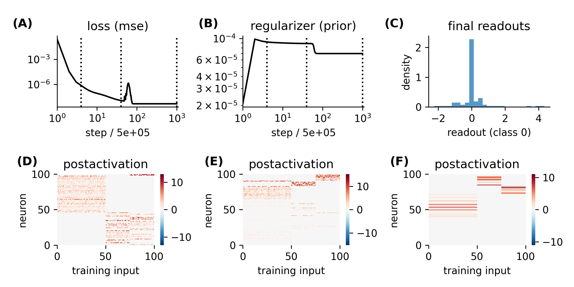
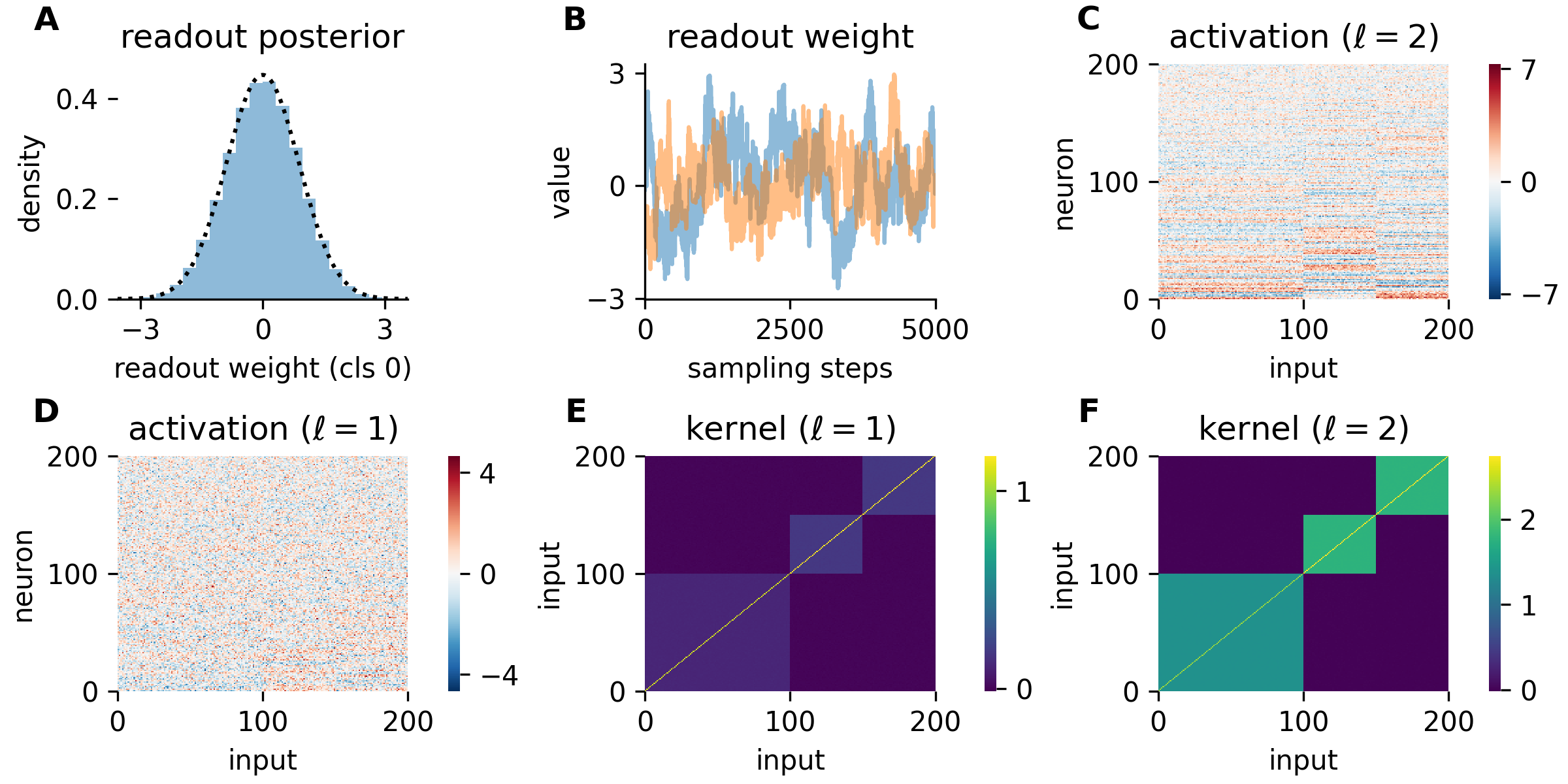
where is a matrix determined by where is the input kernel (see supplement). Gaussianity of the sampled readout weights is shown in Fig. 2(A) using a network with two hidden layers and a toy task (mutually orthogonal inputs, randomly assigned classes, and one-hot targets ) with three classes which are present in the data with ratios . Fig. 2(B) shows that the full posterior is explored during sampling.
The coding scheme is determined by the conditional single neuron posterior of the last layer activations given the readout weights which is also Gaussian, . Its mean codes for the training targets with a strength proportional to the readout weights. Since the readout weights are Gaussian, this leads to an analog coding of the task. A sample of the analog coding scheme is shown in Fig. 2(C) for the two layer network on the toy task.
For the previous layers , the single neuron posterior is independent of and the other layers’ activations, and is Gaussian: for . In all layers, the activation’s covariance is determined by the kernel
| (5) |
The kernel decomposes into a contribution due to the prior and a learned low rank contribution . The strength of the learned part increases across layers, . In the last layer it is , indicating again that the last hidden layer learns strong features. This is in strong contrast to the lazy case where the learned part is suppressed by in all layers [20]. We show a sample of the first layer activations in Fig. 2(D) for the two layer network and the toy task. In contrast to the last layer activations, the learned structure is hardly apparent in the first layer. This is also reflected in the first layer kernel (Fig. 2(E)) where the learned block structure is weak compared to the last layer kernel (Fig. 2(F)).
II.2.2 Generalization
For generalization, we include the dimensional vector of test activations on a set of test inputs , , in the joint posterior. The joint posterior still factorizes across neurons and layers into single neuron posteriors in the last layer and in the previous layers . Like the other single neuron posteriors, is Gaussian for all layers (see supplement).
The kernel for a pair of arbitrary inputs is with the input kernel and the mean predictor which evaluates to
| (6) |
where and . The test kernel is identical to the training kernel (5) except that the training targets are replaced by the predictor. As in the training kernel, the learned part is low rank and becomes more prominent across layers, reaching in the last layer. Despite the strong learned representations, the mean predictor is identical to the lazy case [20] and the GP limit (see supplement). In contrast to the lazy case, the variance of the predictor can be neglected (see supplement).
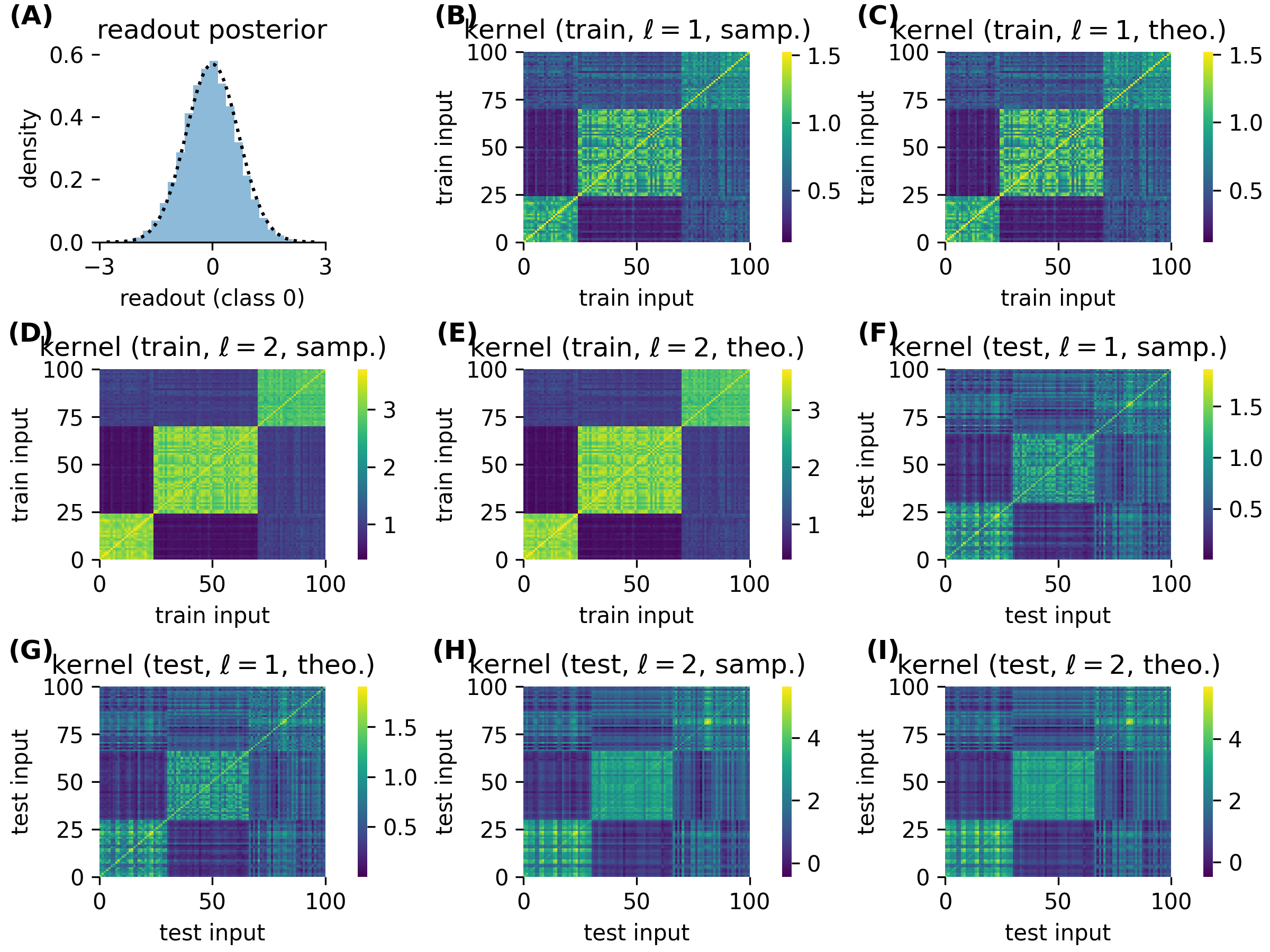
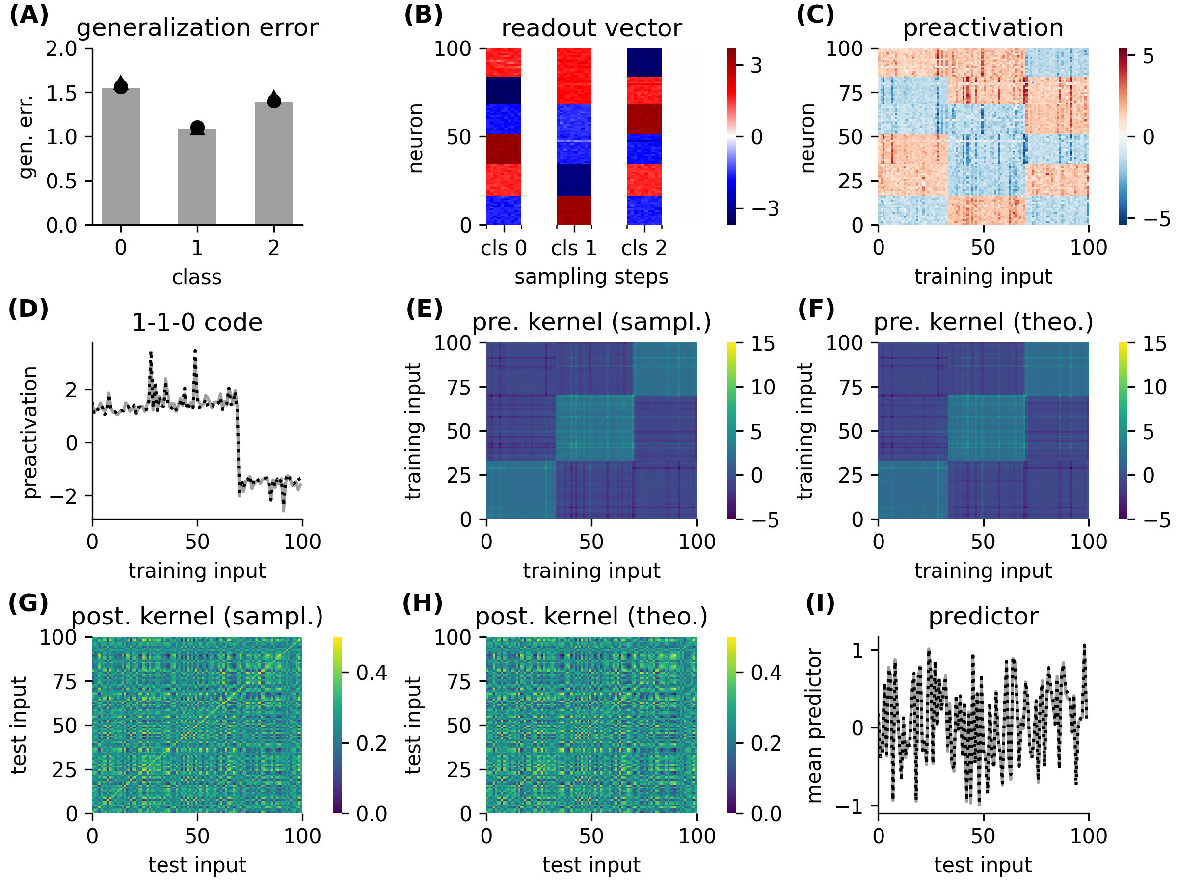
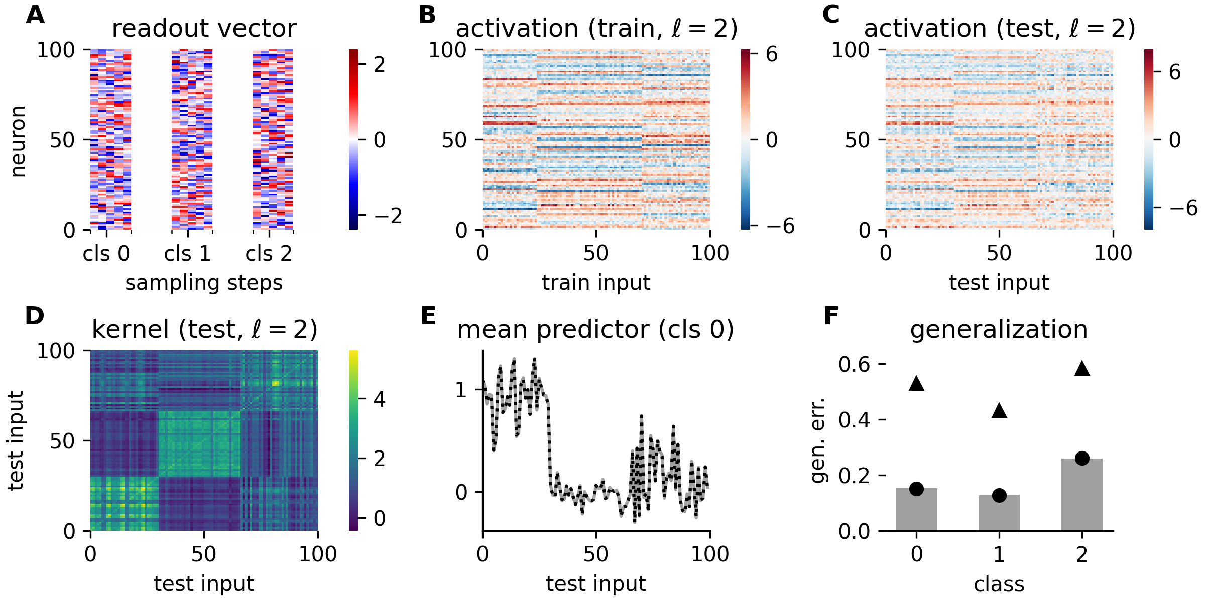
We apply the theory to classification of the first three digits of MNIST. The readout weights are Gaussian and change during sampling (Fig. 3(A)) and the last layer training activations display a clear analog coding of the task (Fig. 3(B)). Thus, the nature of the solution is captured by an analog coding scheme, as in the toy task. On test inputs, the last layer activations still display the analog coding scheme (Fig. 3(C)), which shows that the learned representations generalize. This is confirmed by the test kernel which has a block structure corresponding to the task (Fig. 3(D)). Also the mean predictor generalizes well (Fig. 3(E)) and the class-wise generalization error is reduced compared to the GP theory (Fig. 3(F)). Since the mean predictors are identical, the reduced generalization error is exclusively an effect of the reduced variance of the predictor due to the bias variance decomposition .
II.3 Sigmoidal Networks
For the first nonlinear case, we consider nonnegative sigmoidal networks, . To avoid growth of the readout weights with we set for arbitrary depth.
II.3.1 Training
As in the linear case, the joint posterior of readout weights and preactivations factorizes across layers and neurons, . In contrast to the linear case, the single neuron posteriors are no longer Gaussian.
In particular the readout posterior is drastically different: it is a weighted sum of Dirac deltas
| (7) |
where the weights and the -dimensional vectors are determined jointly for all by a set of self-consistency equations which depend on the training set (see supplement). This means that the vector of readout weights is redundant: each of the neurons has one of possible readout weights and the distribution of readout weights across neurons is given by .
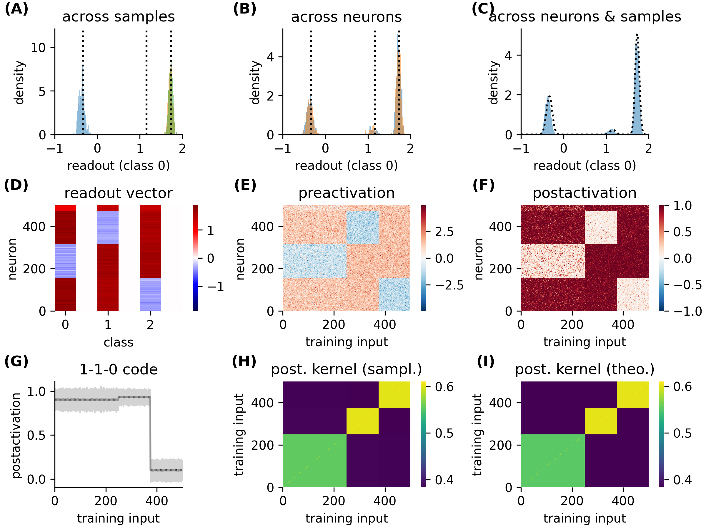
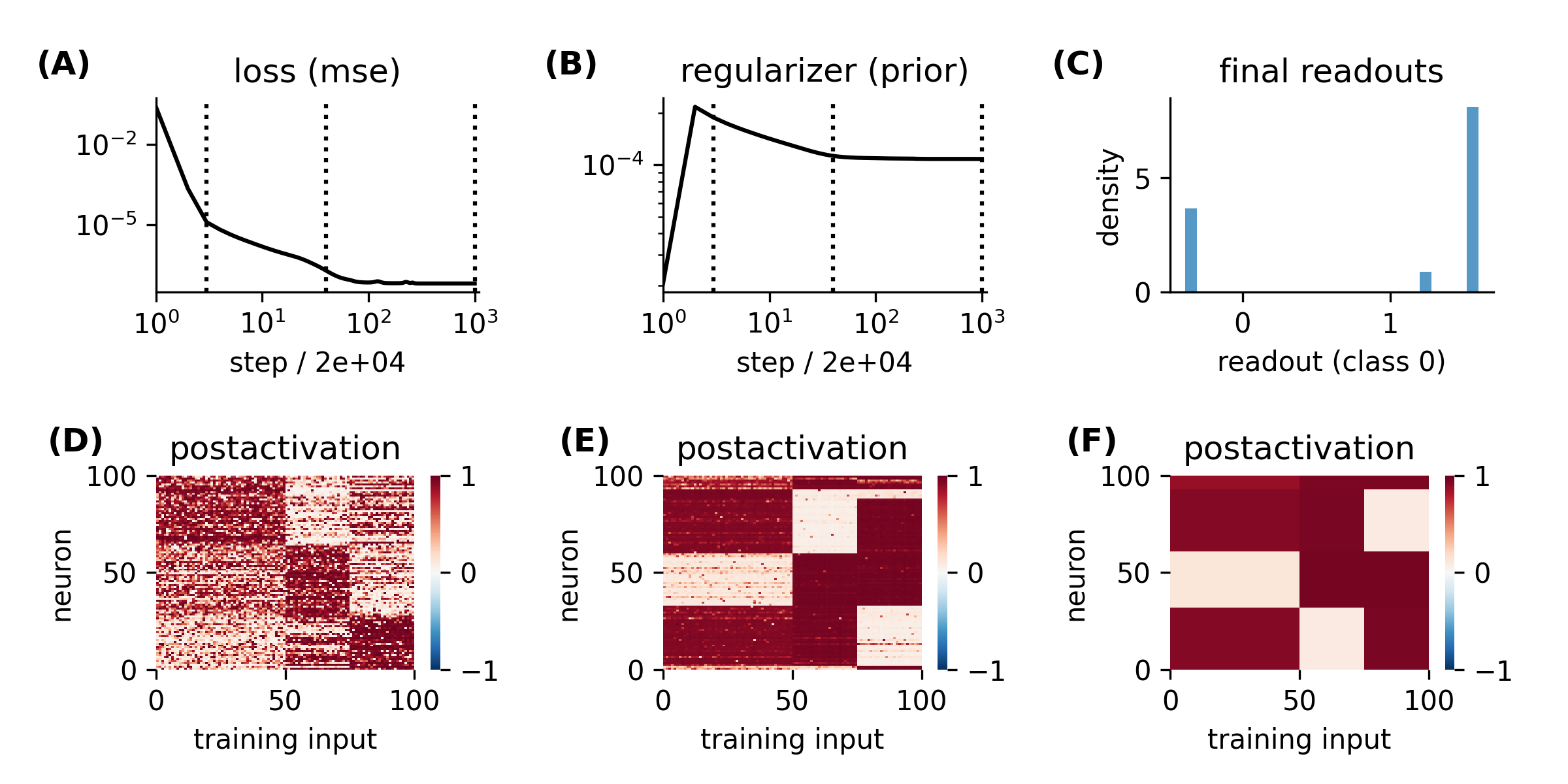
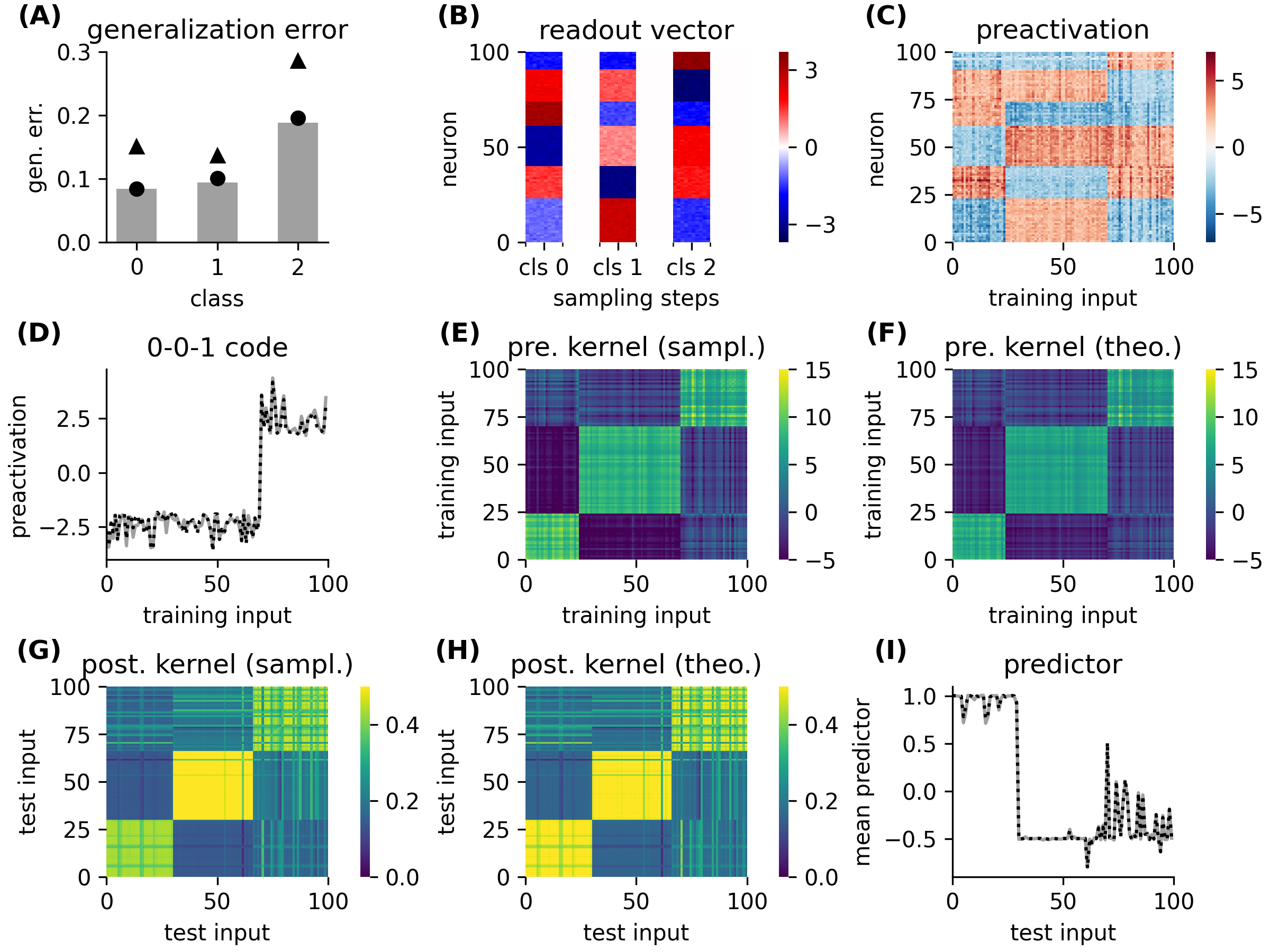
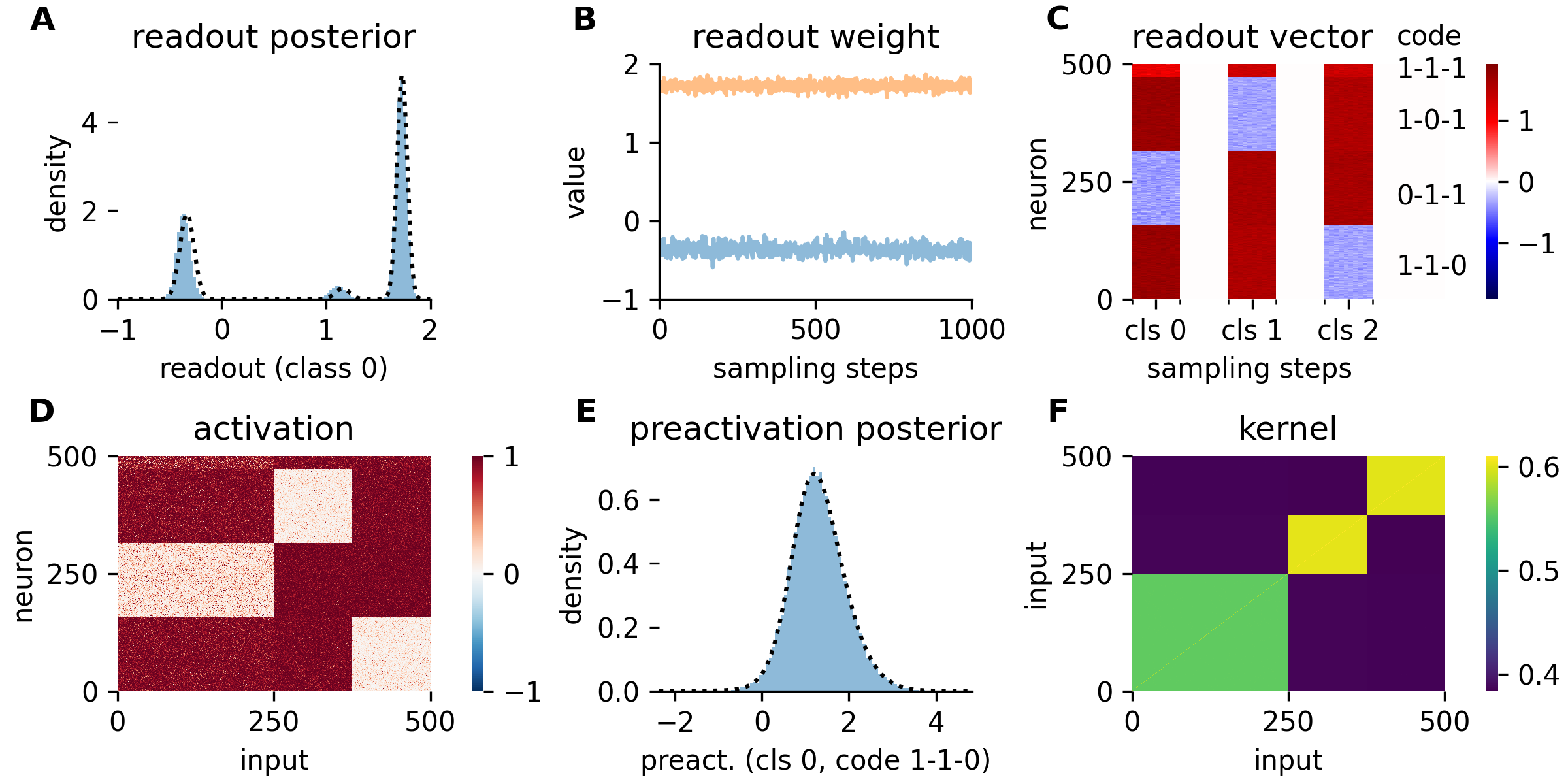
We show the readout posterior for a single layer network on the same toy task with three classes used above in Fig. 4. Across neurons, the posterior splits into disconnected branches which are accurately captured by the theory (Fig. 4(A); here the marginal distribution of the readout weights for the first class is shown). For given neurons, sampling is restricted to one of the branches of the posterior (Fig. 4(B)). Considering all readouts and all neurons simultaneously, the redundant structure of the readout weights becomes apparent (Fig. 4(C)).
The readout weights determine the last layer preactivation through the single neuron conditional distribution . Due to the redundant structure of the readout posterior, a redundant coding scheme emerges in which, on average, a fraction of the neurons exhibit identical preactivation posteriors . Each of the corresponding activations has a pronounced mean that reflects the structure of the task but also significant fluctuations around the mean which do not vanish in the limit of large and (see supplement).
For the single layer network on the toy task, the redundant coding of the task is immediately apparent (Fig. 4(D)) but also the remaining fluctuations are clearly visible (Fig. 4(E)). In this example, there are four codes (Fig. 4(C,D)): 1-1-0, 0-1-1, 1-0-1, and 1-1-1. Note that the presence of code 1-1-1, which is implemented only by a small fraction of neurons, is accurately captured by the theory (Fig. 4(A) middle peak). The relation between the neurons’ activations and their readout weights is straightforward: for neurons with code 1-1-0, the readout weights are positive for classes 0 and 1 and negative for class 2 (Fig. 4(C)), and vice versa for the other codes. Due to the symmetry of the last two classes, which account for of the data each, the readout weights for codes 1-0-1 and 1-1-0 are identical such that in Fig. 4(A) only three peaks are visible but the height of the last peak is doubled. Clearly, the coding scheme with four codes is not the unique solution. Indeed, the theory admits other coding schemes which are, however, unlikely to occur (see supplement).
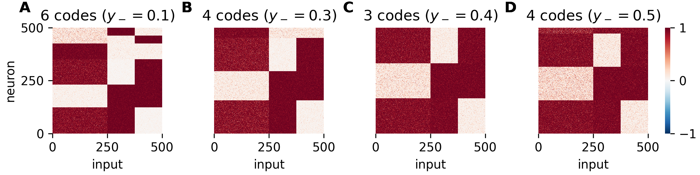
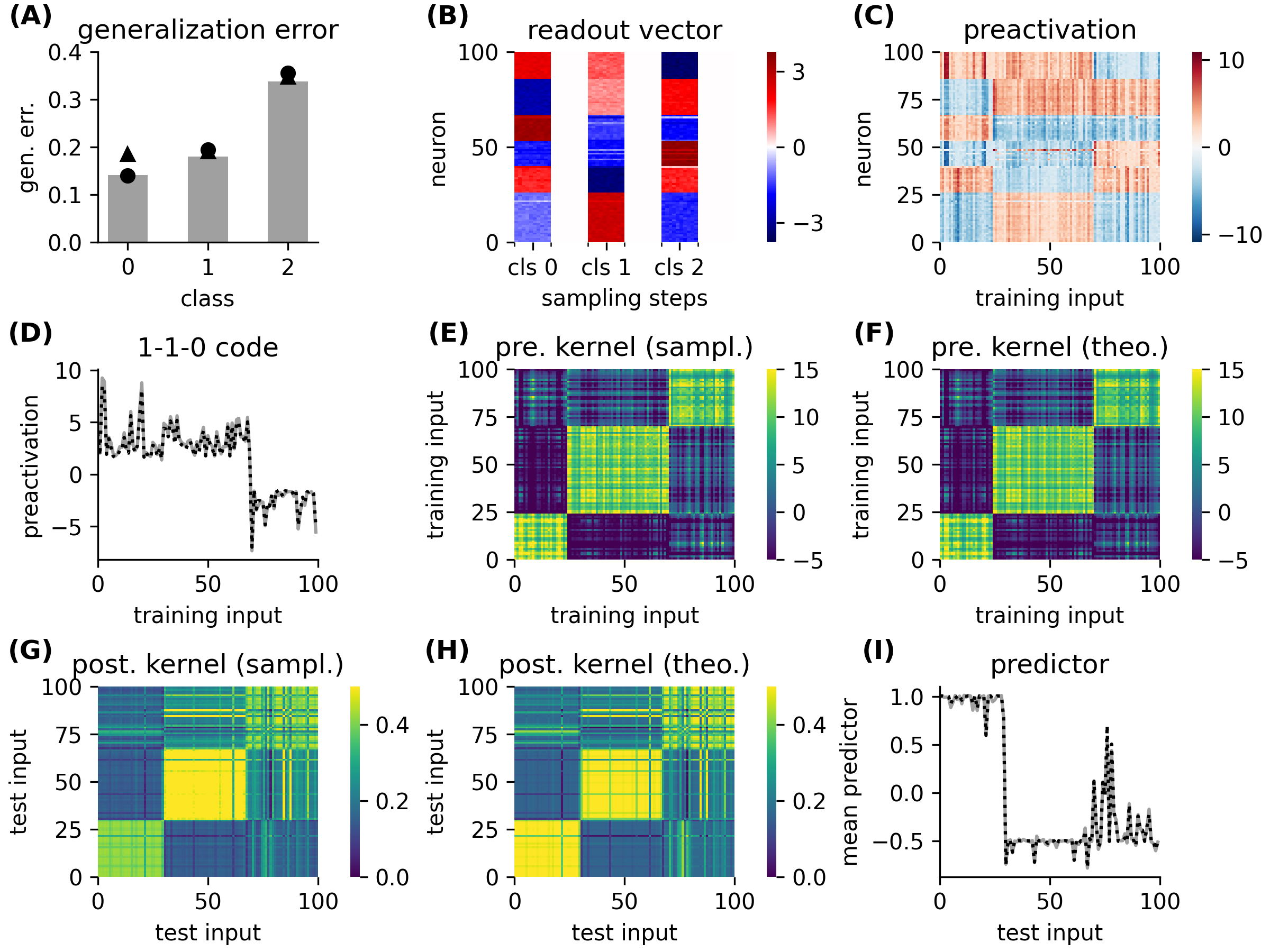
Interestingly, there are transitions in the coding scheme depending on the targets . In Fig. 5 we show the emerging code using the same setup as in Fig. 4 except that the one-hot encoding of the targets increases from to (which was used in Fig. 4), keeping as before. At , the coding scheme contains all six permutations of the 1-0-0 and 1-1-0 codes (Fig. 5(A)). At the codes 0-1-0 and 0-0-1 disappeared (Fig. 5(B)) and at also the code 1-0-0 is lost (Fig. 5(C)). Finally, at the new code 1-1-1 emerged (Fig. 5(D)). Keeping but increasing temperature gradually decreases the strength of the coding scheme until it disappears above a critical temperature (see supplement).
The last layer kernel on training inputs is . Due to the pronounced mean of the activations on the toy task, the kernel possesses a dominant low rank component. For the single layer network and the toy task, this is shown in Fig. 4(F).
A fundamental consequence of the theory is that neuron permutation symmetry is broken in the last layer: due to the disconnected structure of the readout posterior (7), two readout weights from different branches cannot change their identity during sampling (Fig. 4(B)). Furthermore, the readout weights freeze to their value , in strong contrast to the linear case (Fig. 2(B)). Since the readout weights determine the code through , freezing of the readout weights implies freezing of the code, despite the non vanishing fluctuations of preactivations (Fig. 4(E)).
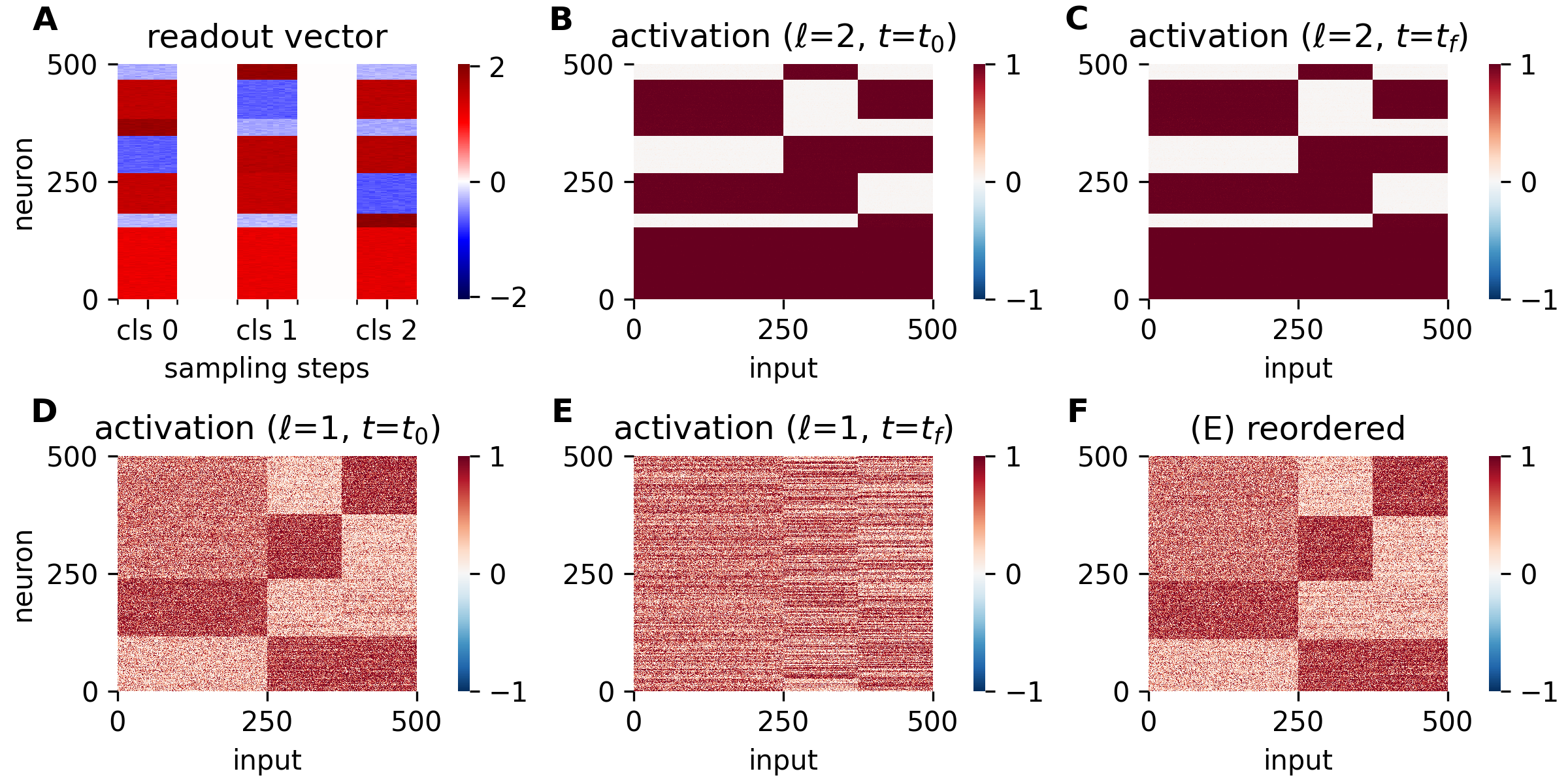
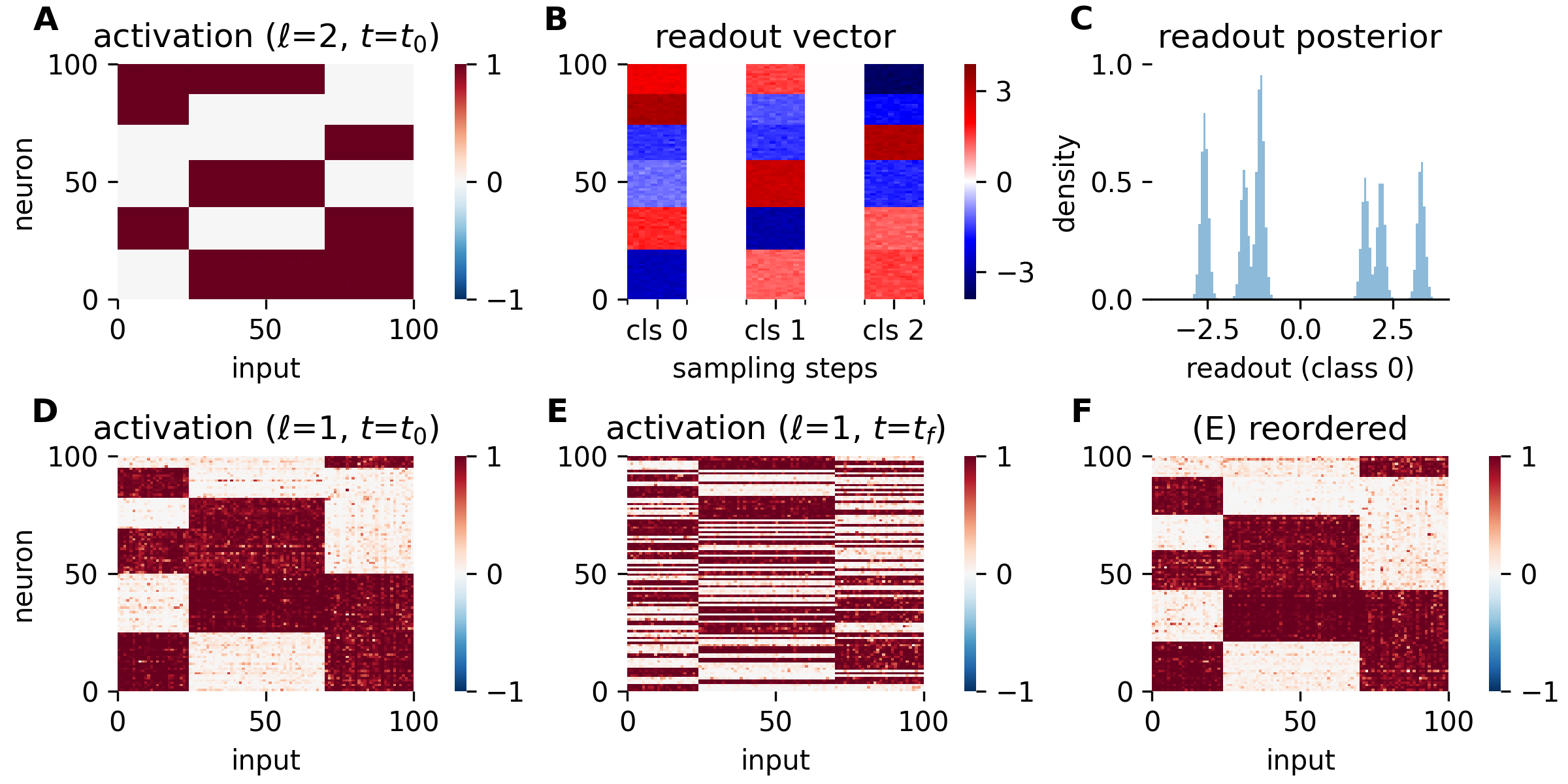
For the lower layers , the posterior is multimodal with each mode corresponding to a code (see supplement). In contrast to the last layer, the code is not frozen since the preactivations are independent from the readout weights. We show the activations of a two layer network on the toy task in Fig. 6. The readout weights are redundant and frozen (Fig. 6(A)) and the last layer activations show a prominent redundant coding of the task (Fig. 6(B)) which does not change during sampling (Fig. 6(C)). In stark contrast, the first layer activations show a redundant coding (Fig. 6(D)) which is not preserved during sampling (Fig. 6(E)). This is a fundamental difference to the last layer where the code is frozen. However, the structure of the code is preserved: after reordering the neurons the solution from the last weight sample is identical to the solution from the first weight sample (Fig. 6(F)).
II.3.2 Generalization
For generalization, we include the preactivations on test inputs . As in the linear case, the posterior factorizes across neurons and layers and the test preactivations only depend on the training preactivations through , , which is Gaussian also for nonlinear networks (see supplement). The resulting mean predictor on a test input is (see supplement)
| (8) |
where and are determined using the training data set, see (7). As in the linear case, the variance of the predictor can be neglected (see supplement).
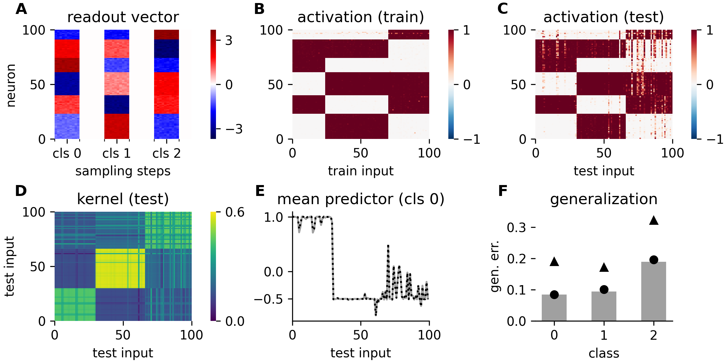
We apply the theory to classification of the first three digits in MNIST with a single hidden layer network. For the theory, we employ the additional approximation of neglecting the fluctuations of the preactivations conditioned on the readout weights. The readout weights are redundant and frozen (Fig. 7(A)) and the training activations display a clear redundant coding scheme (Fig. 7(B)). On test inputs, the redundant coding scheme persists with deviations on certain test inputs (Fig. 7(C)), leading to a clear block structure in the kernel on test data (Fig. 7(D)). The mean predictor is close to the test targets except on particularly difficult test inputs and accurately captured by the theory (Fig. 7(E)); the resulting generalization error is smaller than its counterpart based on the GP theory (Fig. 7(F)). Similar to linear networks, reduction of the generalization error is mainly driven by the reduced variance of the predictor, although in this case also the non-lazy mean predictor performs slightly better.
Using randomly projected MNIST to enable sampling in the regime leads to similar results—a redundant coding scheme on training inputs and good generalization (see supplement). In contrast, using the first three classes of CIFAR10 instead of MNIST while keeping still leads to a redundant coding on the training inputs but the coding scheme is lost on test inputs, indicating that the representations do not generalize well, which is confirmed by a high generalization error (see supplement). Increasing the data set size to all ten classes and the full training set with inputs and using a hidden layer network with neurons improves the generalization to an overall accuracy of ; in this case the last layer training activations show a redundant coding scheme on training inputs which generalize to varying degree to test inputs (see supplement).
II.4 ReLU Networks
Last, we consider ReLU networks, . Here we set as in the linear case owing to the homogeneity of ReLU. For the theory we consider only single hidden layer networks .
II.4.1 Training
We start with the representations on training data. The nature of the posterior is fundamentally different compared to the previous cases: it factorizes into a small number of outlier neurons and a remaining bulk of neurons, .
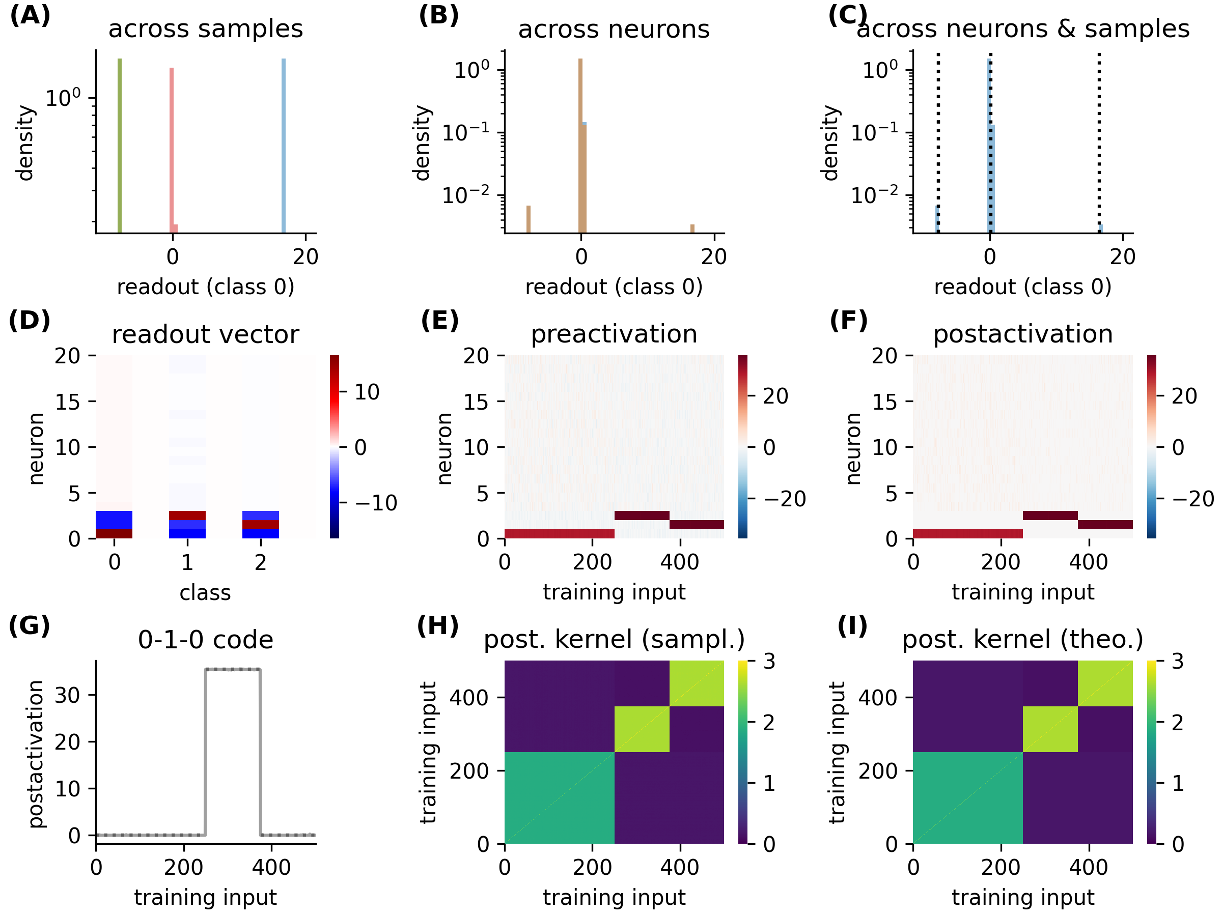
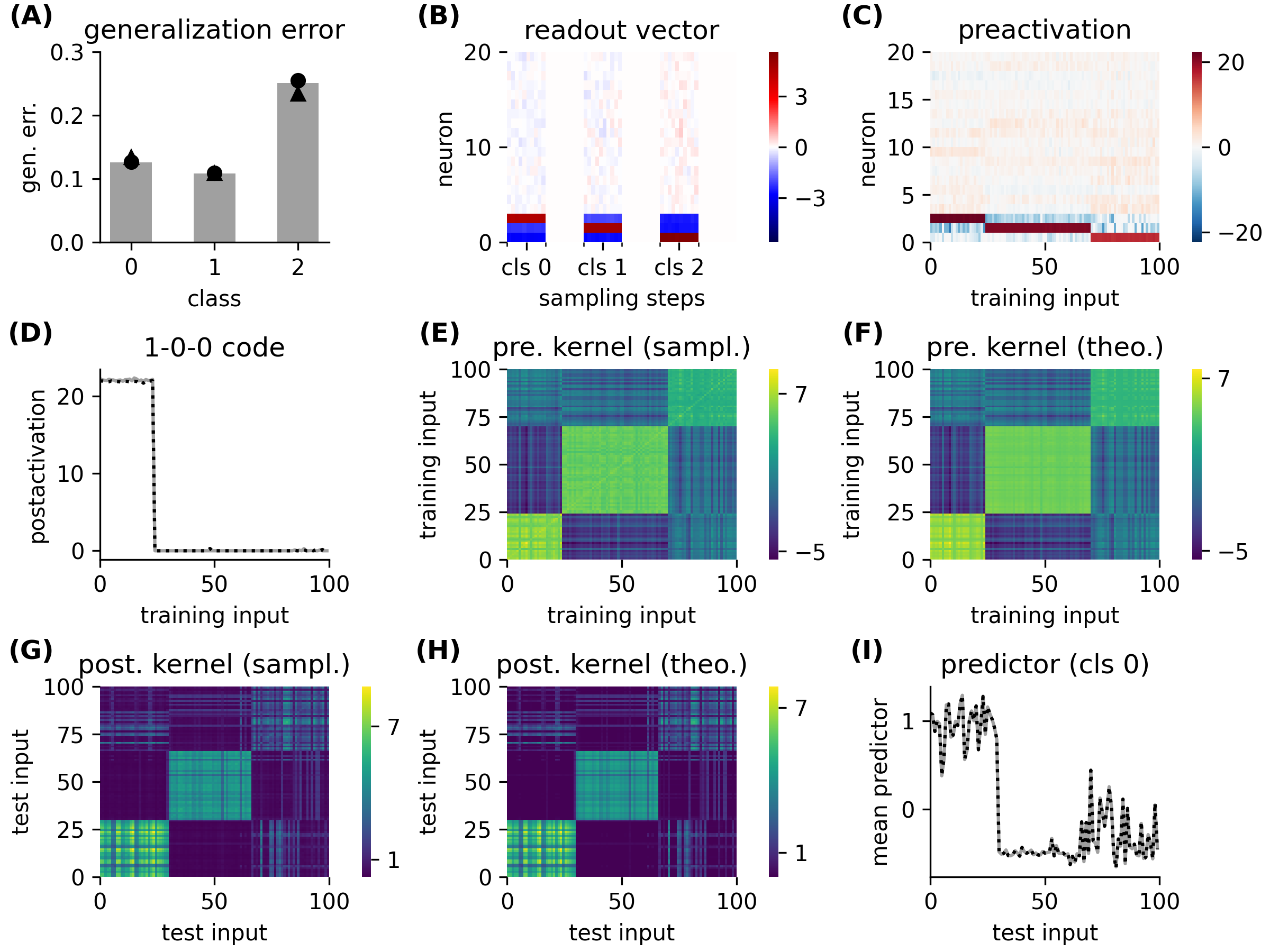
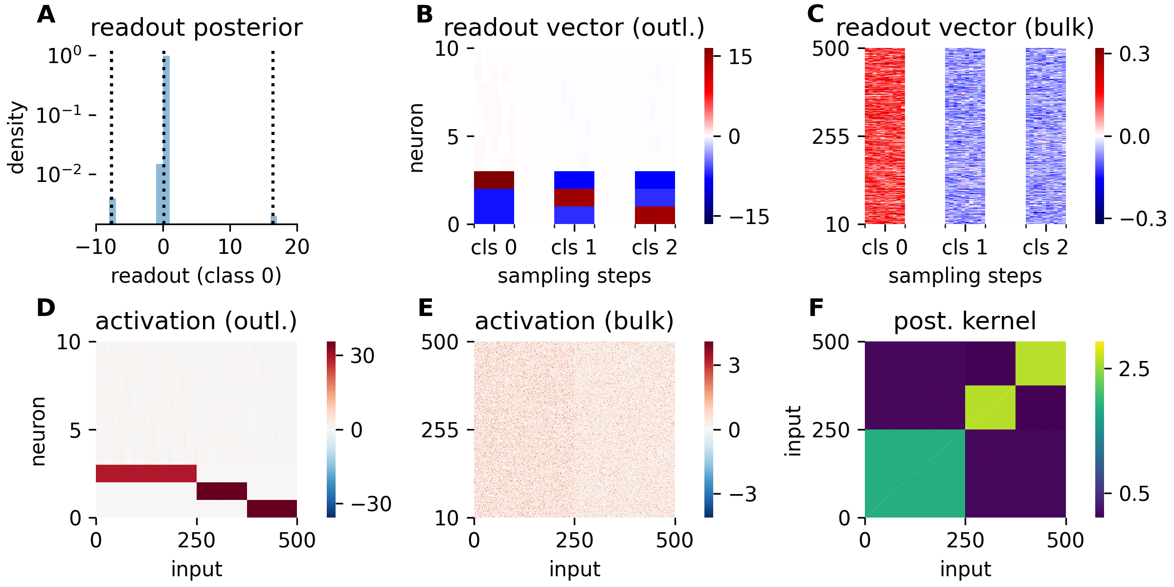
The readout weight posteriors of the outlier neurons are Dirac deltas at values, . For the bulk neurons , the readout weight posterior is also a Dirac delta but the values are , . The values of and are determined self-consistently with the training data set (see supplement). The readout weight posterior on the toy task is shown in Fig. 8(A-C). In this case there are outliers, corresponding to the classes. Considering the distribution across neurons highlights the difference in magnitude between the bulk and the outliers and demonstrates the match between theory and sampling (Fig. 8(A)). In the plot, only two outliers are visible because the two negative outliers have identical value due to the symmetry of the last two classes, leading to a single peak with twice with a doubled height. During sampling, both the outlier (Fig. 8(B)) and the bulk (Fig. 8(C)) readout weights are frozen to their respective values.
The last layer representations are determined by the conditional distribution of the preactivations. For the outliers, this distribution is a Dirac delta at values, . Thus, for the outlier neurons the activations and readout weights jointly overcome the non-lazy scaling. All neurons of the bulk are identically distributed according to a non-Gaussian posterior . In particular, this means that the neurons from the bulk share the same code. However, if there are multiple classes , or a single class with positive and negative targets, a single code is not sufficient to solve the task. Thus, the outliers must carry the task relevant information leading to a sparse coding scheme. On the toy task, the outliers code for a single class each (Fig. 8(D)) while the bulk is largely task agnostic (Fig. 8(E)). The relation between readout weights and activations is straightforward: readout weights for the outlier neurons are positive for the coded class and negative otherwise (Fig. 8(B,D)).
The kernel comprises contributions due to the outliers and the bulk: . The contribution due to the outliers is because their activations are which cancels the in front of the kernel (3). On the toy task, the outlier contribution leads to a dominant low rank component (Fig. 8(F)).
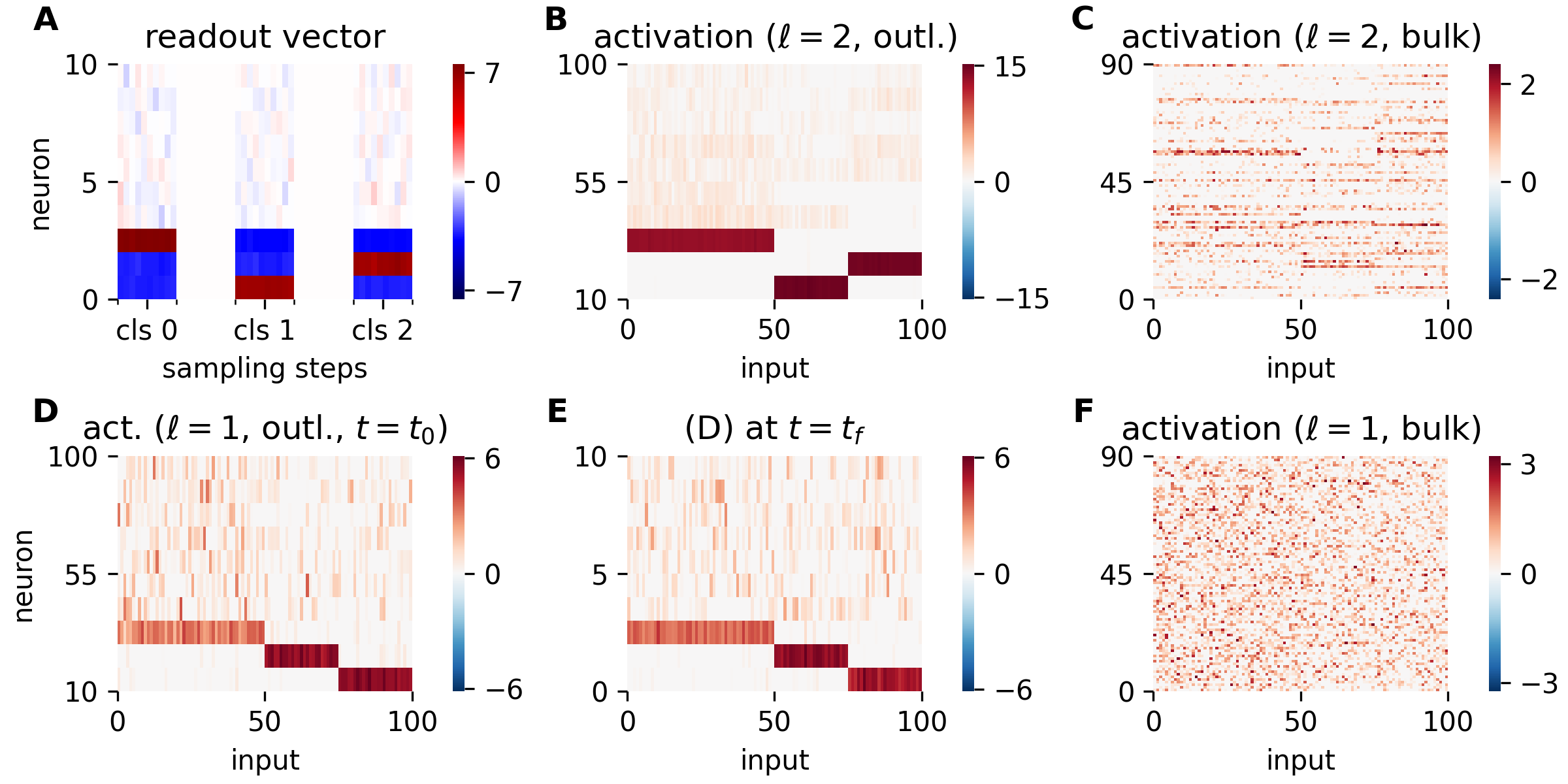
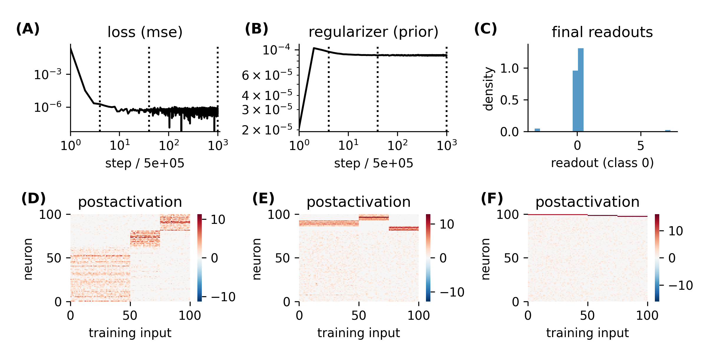
We investigate deeper networks numerically. For two hidden layers () on the toy task, the readout weights contain three outliers (Fig. 9(A)) and the last layer shows a sparse coding of the task with three outlier neurons coding for one class each (Fig. 9(B)). A difference to the single layer case is that the bulk also shows a weak coding for the task (Fig. 9(C)). In the first layer there are again three outliers coding for one class each (Fig. 9(D)). Unlike in sigmoidal networks the codes are frozen, i.e., the outliers do not change identity or switch with the bulk (Fig. 9(E)). Finally, the bulk in the first layer is task agnostic (Fig. 9(F)).
II.4.2 Generalization
For generalization we include the test preactivations on test inputs . As in the previous cases, this leads to the Gaussian conditional distribution . The predictor on a test input is
| (9) |
with for . As for the other nonlinearities, the predictor variance can be neglected.
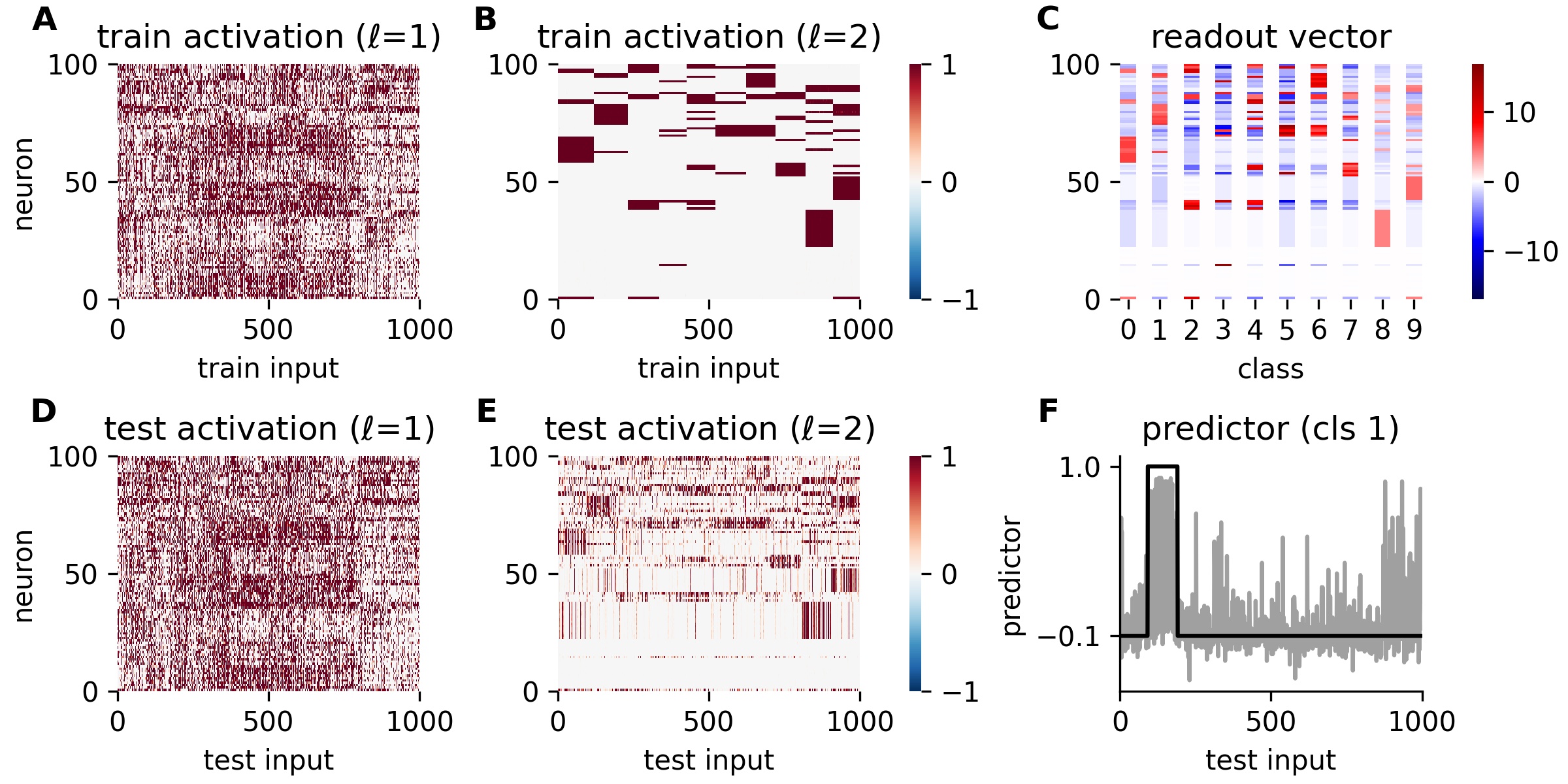
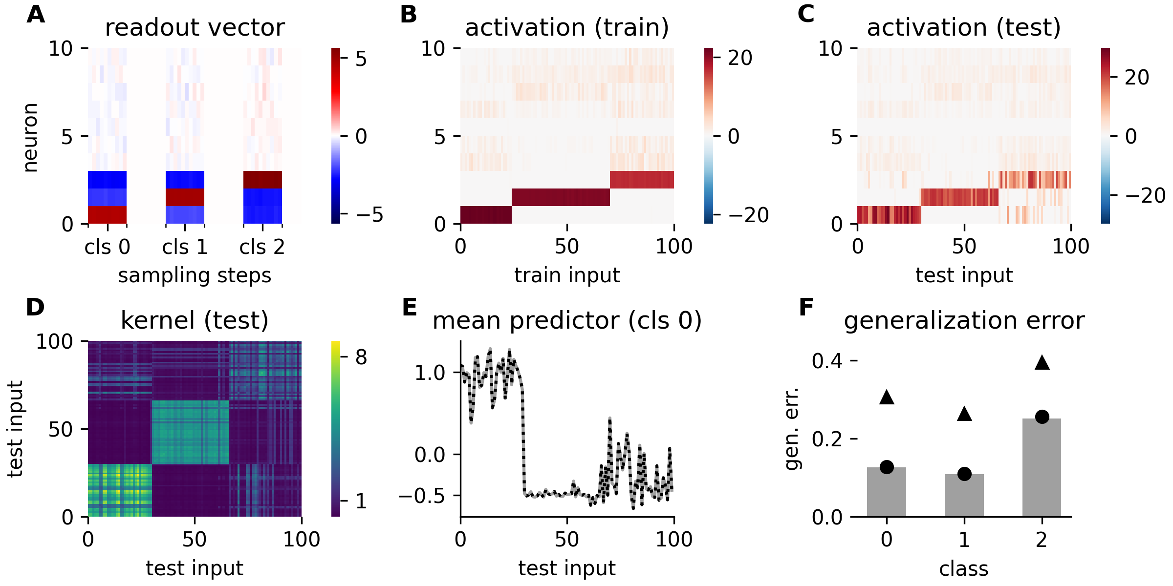
On the first three digits of MNIST, the readout weights are sparse (Fig. 10(A)) and the training (Fig. 10(B)) as well as test (Fig. 10(C)) activations exhibit three outliers which code for one class each. The kernel on test data displays a clear block structure (Fig. 10(D)) due to the outliers. For the theory, we neglect the bulk to make it tractable. Despite this approximation, the predictor is accurately captured by the theory (Fig. 10(E)). In terms of the generalization error, the nonlazy network outperforms the GP predictor (Fig. 10(F)) due to the reduction of the predictor variance.
III Discussion
We developed a theory for the weight posterior of non-lazy networks in the limit of infinite width and data set size, from which we derived analytical expressions for the single neuron posteriors of the readout weights and the preactivations on training and test inputs. These single neuron posteriors revealed that the learned representations are embedded into the network using distinct coding schemes. Furthermore, we used the single neuron posteriors to derive the mean predictor and the mean kernels on training and test inputs. We applied the theory to two classification tasks: a simple toy model using orthogonal data and random labels to highlight the coding schemes and image classification using MNIST and CIFAR10 to investigate generalization. In both cases, the theoretical results are in excellent agreement with empirical samples from the weight posterior.
Coding Schemes
We show that the embedding of learned representations by the neurons exhibits a remarkable structure: a coding scheme where distinct populations of neurons are characterized by the subset of classes that activate them. The details of the coding scheme depend strongly on the nonlinearity: linear networks display an analog coding scheme where all neurons code for all classes in a graded manner (Figs. 2, 3), sigmoidal networks display a redundant coding scheme where large populations of neurons are active on specific combinations of classes (Figs. 4, 6, 7), and ReLU networks display a sparse coding scheme in which a few individual neurons are active on specific classes while the remaining neurons are task agnostic (Figs. 8, 9, 10). In networks with multiple hidden layers, the coding scheme appears in all layers but is sharpened across layers; the coding scheme in the last layer remains the same as in the single layer case (Figs. 6, 9).
Why were the coding schemes not previously observed? Compared to standard training protocols, there are two main differences: (1) the sampling from the posterior, i.e., training for a long time with added noise, and (2) the data set size dependent strength of the readout weight variance, which corresponds to a data set size dependent regularization using weight decay. As we show in the supplement, training without noise also leads to sparse or redundant coding schemes. Thus, the data set size dependent regularization seems to be crucial which is, to the best of our knowledge, not commonly used in practice.
Permutation Symmetry Breaking
The coding schemes determine the structure of a typical solution sampled from the weight posterior, e.g., for sigmoidal networks a solution with a redundant coding scheme. Due to the neuron permutation symmetry of the posterior, each typical solution has permuted counterparts which are also typical solutions. Permutation symmetry breaking occurs if these permuted solutions are disconnected in solution space, i.e., if the posterior contains high barriers between the permuted solutions.
In sigmoidal and ReLU networks, permutation symmetry is broken. The theoretical signature of this symmetry breaking is the disconnected structure of the posterior of the readout weights where the different branches are separated by high barriers. Numerically, symmetry breaking is evidenced by the fact that, at equilibrium, neurons do not change their coding identity with sampling time. We note that for the readout weights, the symmetry broken phase is also a frozen state, namely not only the coding structure is fixed but also there are no fluctuations in the magnitude of each weight (Figs. 4, 6, 8, 9). In contrast, activations in the hidden layer, also constant in their coding, do exhibit residual temporal fluctuations around a pronounced mean (Figs. 4, 6) which carries the task relevant information.
Interestingly, the situation is more involved in networks with two hidden layers. In the first layer, permutation symmetry is broken and the neurons’ code is frozen in ReLU networks (Fig. 9) but not in sigmoidal networks (Fig. 6). In the latter case, the typical solution has a prominent coding scheme but individual neurons switch their code during sampling (Fig. 6).
Symmetry breaking has been frequently discussed in the context of learning in artificial neural networks, for example replica symmetry breaking in perceptrons with binary weights [43, 44, 45], permutation symmetry breaking in fully connected networks [46, 47] and restricted Boltzmann machines [48], or continuous symmetry breaking of the “kinetic energy” (reflecting the learning rule) [49, 50]. Furthermore, [51] links breaking of parity symmetry to feature learning, albeit in a different scaling limit. The role of an intact (not broken) permutation symmetry has been explored in the context of the connectedness of the loss landscape [52, 53, 54]. Here, we establish, for the first time, a direct link between symmetry breaking and the nature of the neural representations.
Neural Collapse
The redundant coding scheme in sigmoidal network and the sparse coding scheme in ReLU networks are closely related to the phenomenon of neural collapse [55]. The two main properties of collapse are (1) vanishing variability across inputs from the same class of the last layer postactivations and (2) last layer postactivations forming an equiangular tight frame (centered class means are equidistant and equiangular with maximum angle). There are two additional properties which, however, follow from the first two under minimal assumptions [55]. We note that collapse is determined only on training data in the original definition.
Formally, the first property of collapse is violated in the non-lazy networks investigated here due to the non vanishing across-neuron variability of the activations given the readout weights. However, the mean activations conditional on the readout weights, which carry the task relevant information, generate an equiangular tight frame in both sigmoidal and ReLU networks. This creates an interesting link to empirically trained networks where neural collapse has been shown to occur under a wide range of conditions [55, 56].
Neglecting the non-vanishing variability, the main difference between neural collapse and the coding schemes is that the latter impose a more specific structure. Technically, the equiangular tight frame characterizing neural collapse is invariant under orthogonal transformations while the coding schemes are invariant under permutations, which is a subset of the orthogonal transformations. This additional structure makes the representations highly interpretable in terms of a neural code—conversely, applying, e.g., a rotation in neuron space to the redundant or sparse coding scheme would hide the immediately apparent structure of the solution.
Representation Learning and Generalization
The case of non-lazy linear networks makes an interesting point about the interplay between feature learning and generalization: although the networks learn strong, task-dependent representations, the mean predictor is identical to the Gaussian Process limit where the features are random. The only difference between non-lazy networks and random features is a reduction in the predictor variance. Thus, this provides an explicit example where feature learning only mildly helps generalization through reduction of the predictor variance.
More generally, in all examples the improved performance of nonlazy networks (Figs. 3, 7, 10) is mainly driven by the reduction of the predictor variance; the mean predictor does not generalize significantly better than a predictor based on random features. This shows an important limitation of our work: in order to achieve good generalization performance, it might be necessary to consider deeper nonlinear architectures or additional structure in the model.
While the learned representations might not necessarily help generalization on the trained task, they can still be useful for few shot learning of a novel task [57, 58, 59, 60]. Indeed, neural collapse has been shown to be helpful for transfer learning if neural collapse still holds (approximately) on inputs from the novel classes [61]. Due to the relation between coding schemes and neural collapse, this suggests that the learned representations investigated here are useful for downstream task—if the nature of the solution does not change on the new inputs. This remains to be systematically explored.
Lazy vs. Non-Lazy Regime
The definition of lazy vs. non-lazy regime is subtle. Originally, the lazy regime was defined by the requirement that the learned changes in the weights affect the final output only linearly [62]. This implies that the learned changes in the representations are weak since changes in the hidden layer weights nonlinearly affect the final output. To overcome the weak representation learning, [38, 39] define the non-lazy regime as changes of the features during the first steps of gradient descent. This definition leads to an initialization where the readout scales its inputs with [39]. However, the scaling might change during training—which is not captured by a definition at initialization.
We here define the non-lazy regime such that the readout scales its inputs with after learning, i.e., under the posterior. Importantly, we prevent that the readout weights overcome the scaling by growing their norm, which leads to the requirement of a decreasing prior variance of the readout weights with increasing . The definition implies that strong representations are learned: the readout weights must be aligned with the last layer’s features on all training inputs, which is not the case for random features.
Acknowledgements.
Many helpful discussions with Qianyi Li and feedback on the manuscript by Lorenzo Tiberi, Chester Mantel, Kazuki Irie, and Haozhe Shan are gratefully acknowledged. This research was supported by the Swartz Foundation, the Gatsby Charitable Foundation, and in part by grant NSF PHY-1748958 to the Kavli Institute for Theoretical Physics (KITP).References
- Bengio et al. [2013] Y. Bengio, A. Courville, and P. Vincent, IEEE Trans. Pattern Anal. Mach. Intell. 35, 1798–1828 (2013).
- LeCun et al. [2015] Y. LeCun, Y. Bengio, and G. Hinton, Nature 521, 436 (2015).
- Goodfellow et al. [2016] I. Goodfellow, Y. Bengio, and A. Courville, Deep Learning (MIT Press, 2016) http://www.deeplearningbook.org.
- Zhang et al. [2017] C. Zhang, S. Bengio, M. Hardt, B. Recht, and O. Vinyals, in International Conference on Learning Representations (2017).
- Zhang et al. [2021] C. Zhang, S. Bengio, M. Hardt, B. Recht, and O. Vinyals, Commun. ACM 64, 107–115 (2021).
- Belkin et al. [2019] M. Belkin, D. Hsu, S. Ma, and S. Mandal, Proceedings of the National Academy of Sciences 116, 15849 (2019).
- Nakkiran et al. [2020] P. Nakkiran, G. Kaplun, Y. Bansal, T. Yang, B. Barak, and I. Sutskever, in International Conference on Learning Representations (2020).
- Belkin [2021] M. Belkin, Acta Numerica 30, 203–248 (2021).
- Shwartz-Ziv et al. [2024] R. Shwartz-Ziv, M. Goldblum, A. Bansal, C. B. Bruss, Y. LeCun, and A. G. Wilson, Just how flexible are neural networks in practice? (2024), arXiv:2406.11463 .
- MacKay [2003] D. J. MacKay, Information theory, inference and learning algorithms (Cambridge university press, 2003).
- Bahri et al. [2020] Y. Bahri, J. Kadmon, J. Pennington, S. S. Schoenholz, J. Sohl-Dickstein, and S. Ganguli, Annu. Rev. Condens. Matter Phys. 11, 501 (2020).
- Neal [1996] R. M. Neal, Bayesian Learning for Neural Networks (Springer New York, 1996).
- Williams [1996] C. Williams, in Advances in Neural Information Processing Systems, Vol. 9, edited by M. Mozer, M. Jordan, and T. Petsche (MIT Press, 1996).
- Lee et al. [2018] J. Lee, J. Sohl-Dickstein, J. Pennington, R. Novak, S. Schoenholz, and Y. Bahri, in International Conference on Learning Representations (2018).
- Matthews et al. [2018] A. G. d. G. Matthews, J. Hron, M. Rowland, R. E. Turner, and Z. Ghahramani, in International Conference on Learning Representations (2018).
- Yang [2019] G. Yang, in Advances in Neural Information Processing Systems, Vol. 32, edited by H. Wallach, H. Larochelle, A. Beygelzimer, F. d'Alché-Buc, E. Fox, and R. Garnett (Curran Associates, Inc., 2019).
- Naveh et al. [2021] G. Naveh, O. Ben David, H. Sompolinsky, and Z. Ringel, Phys. Rev. E 104, 064301 (2021).
- Segadlo et al. [2022] K. Segadlo, B. Epping, A. van Meegen, D. Dahmen, M. Krämer, and M. Helias, Journal of Statistical Mechanics: Theory and Experiment 2022, 103401 (2022).
- Hron et al. [2022] J. Hron, R. Novak, J. Pennington, and J. Sohl-Dickstein, in Proceedings of the 39th International Conference on Machine Learning, Proceedings of Machine Learning Research, Vol. 162, edited by K. Chaudhuri, S. Jegelka, L. Song, C. Szepesvari, G. Niu, and S. Sabato (PMLR, 2022) pp. 8926–8945.
- Li and Sompolinsky [2021] Q. Li and H. Sompolinsky, Physical Review X 11, 031059 (2021).
- Naveh and Ringel [2021] G. Naveh and Z. Ringel, in Advances in Neural Information Processing Systems, edited by A. Beygelzimer, Y. Dauphin, P. Liang, and J. W. Vaughan (2021).
- Zavatone-Veth et al. [2022] J. A. Zavatone-Veth, W. L. Tong, and C. Pehlevan, Phys. Rev. E 105, 064118 (2022).
- Cui et al. [2023] H. Cui, F. Krzakala, and L. Zdeborova, in Proceedings of the 40th International Conference on Machine Learning, Proceedings of Machine Learning Research, Vol. 202, edited by A. Krause, E. Brunskill, K. Cho, B. Engelhardt, S. Sabato, and J. Scarlett (PMLR, 2023) pp. 6468–6521.
- Hanin and Zlokapa [2023] B. Hanin and A. Zlokapa, Proceedings of the National Academy of Sciences 120, e2301345120 (2023).
- Pacelli et al. [2023] R. Pacelli, S. Ariosto, M. Pastore, F. Ginelli, M. Gherardi, and P. Rotondo, Nature Machine Intelligence 5, 1497–1507 (2023).
- Fischer et al. [2024] K. Fischer, J. Lindner, D. Dahmen, Z. Ringel, M. Krämer, and M. Helias, Critical feature learning in deep neural networks (2024), arXiv:2405.10761 [cond-mat.dis-nn] .
- Chizat et al. [2019] L. Chizat, E. Oyallon, and F. Bach, in Advances in Neural Information Processing Systems, Vol. 32, edited by H. Wallach, H. Larochelle, A. Beygelzimer, F. d'Alché-Buc, E. Fox, and R. Garnett (Curran Associates, Inc., 2019).
- Woodworth et al. [2020] B. Woodworth, S. Gunasekar, J. D. Lee, E. Moroshko, P. Savarese, I. Golan, D. Soudry, and N. Srebro, in Proceedings of Thirty Third Conference on Learning Theory, Proceedings of Machine Learning Research, Vol. 125, edited by J. Abernethy and S. Agarwal (PMLR, 2020) pp. 3635–3673.
- Geiger et al. [2020] M. Geiger, S. Spigler, A. Jacot, and M. Wyart, Journal of Statistical Mechanics: Theory and Experiment 2020, 113301 (2020).
- Yaida [2020] S. Yaida, in Proceedings of The First Mathematical and Scientific Machine Learning Conference, Proceedings of Machine Learning Research, Vol. 107, edited by J. Lu and R. Ward (PMLR, 2020) pp. 165–192.
- Dyer and Gur-Ari [2020] E. Dyer and G. Gur-Ari, in International Conference on Learning Representations (2020).
- Zavatone-Veth et al. [2021] J. A. Zavatone-Veth, A. Canatar, B. Ruben, and C. Pehlevan, in Advances in Neural Information Processing Systems, edited by A. Beygelzimer, Y. Dauphin, P. Liang, and J. W. Vaughan (2021).
- Roberts et al. [2022] D. A. Roberts, S. Yaida, and B. Hanin, The Principles of Deep Learning Theory (Cambridge University Press, 2022).
- Mei et al. [2018] S. Mei, A. Montanari, and P.-M. Nguyen, Proceedings of the National Academy of Sciences 115, E7665 (2018).
- Chizat and Bach [2018] L. Chizat and F. Bach, in Advances in Neural Information Processing Systems, Vol. 31, edited by S. Bengio, H. Wallach, H. Larochelle, K. Grauman, N. Cesa-Bianchi, and R. Garnett (Curran Associates, Inc., 2018).
- Rotskoff and Vanden-Eijnden [2018] G. Rotskoff and E. Vanden-Eijnden, in Advances in Neural Information Processing Systems, Vol. 31, edited by S. Bengio, H. Wallach, H. Larochelle, K. Grauman, N. Cesa-Bianchi, and R. Garnett (Curran Associates, Inc., 2018).
- Sirignano and Spiliopoulos [2020] J. Sirignano and K. Spiliopoulos, Stochastic Processes and their Applications 130, 1820 (2020).
- Yang and Hu [2021] G. Yang and E. J. Hu, in Proceedings of the 38th International Conference on Machine Learning, Proceedings of Machine Learning Research, Vol. 139, edited by M. Meila and T. Zhang (PMLR, 2021) pp. 11727–11737.
- Bordelon and Pehlevan [2022] B. Bordelon and C. Pehlevan, in Advances in Neural Information Processing Systems (2022).
- Bordelon and Pehlevan [2023] B. Bordelon and C. Pehlevan, in Thirty-seventh Conference on Neural Information Processing Systems (2023).
- Cortes et al. [2012] C. Cortes, M. Mohri, and A. Rostamizadeh, Journal of Machine Learning Research 13, 795 (2012).
- Kornblith et al. [2019] S. Kornblith, M. Norouzi, H. Lee, and G. Hinton, in Proceedings of the 36th International Conference on Machine Learning, Proceedings of Machine Learning Research, Vol. 97, edited by K. Chaudhuri and R. Salakhutdinov (PMLR, 2019) pp. 3519–3529.
- Krauth and Mézard [1989] W. Krauth and M. Mézard, Journal de Physique 50, 3057–3066 (1989).
- Seung et al. [1992] H. S. Seung, H. Sompolinsky, and N. Tishby, Phys. Rev. A 45, 6056 (1992).
- Watkin et al. [1993] T. L. H. Watkin, A. Rau, and M. Biehl, Rev. Mod. Phys. 65, 499 (1993).
- Barkai et al. [1992] E. Barkai, D. Hansel, and H. Sompolinsky, Phys. Rev. A 45, 4146 (1992).
- Engel et al. [1992] A. Engel, H. M. Köhler, F. Tschepke, H. Vollmayr, and A. Zippelius, Phys. Rev. A 45, 7590 (1992).
- Hou et al. [2019] T. Hou, K. Y. M. Wong, and H. Huang, Journal of Physics A: Mathematical and Theoretical 52, 414001 (2019).
- Kunin et al. [2021] D. Kunin, J. Sagastuy-Brena, S. Ganguli, D. L. Yamins, and H. Tanaka, in International Conference on Learning Representations (2021).
- Tanaka and Kunin [2021] H. Tanaka and D. Kunin, in Advances in Neural Information Processing Systems, Vol. 34, edited by M. Ranzato, A. Beygelzimer, Y. Dauphin, P. Liang, and J. W. Vaughan (Curran Associates, Inc., 2021) pp. 25646–25660.
- Rubin et al. [2024] N. Rubin, I. Seroussi, and Z. Ringel, in The Twelfth International Conference on Learning Representations (2024).
- Brea et al. [2019] J. Brea, B. Simsek, B. Illing, and W. Gerstner, Weight-space symmetry in deep networks gives rise to permutation saddles, connected by equal-loss valleys across the loss landscape (2019), arXiv:1907.02911 [cs.LG] .
- Simsek et al. [2021] B. Simsek, F. Ged, A. Jacot, F. Spadaro, C. Hongler, W. Gerstner, and J. Brea, in Proceedings of the 38th International Conference on Machine Learning, Proceedings of Machine Learning Research, Vol. 139, edited by M. Meila and T. Zhang (PMLR, 2021) pp. 9722–9732.
- Entezari et al. [2022] R. Entezari, H. Sedghi, O. Saukh, and B. Neyshabur, in International Conference on Learning Representations (2022).
- Papyan et al. [2020] V. Papyan, X. Y. Han, and D. L. Donoho, Proceedings of the National Academy of Sciences 117, 24652 (2020).
- Han et al. [2022] X. Han, V. Papyan, and D. L. Donoho, in International Conference on Learning Representations (2022).
- Fei-Fei et al. [2006] L. Fei-Fei, R. Fergus, and P. Perona, IEEE Transactions on Pattern Analysis and Machine Intelligence 28, 594 (2006).
- Vinyals et al. [2016] O. Vinyals, C. Blundell, T. Lillicrap, k. kavukcuoglu, and D. Wierstra, in Advances in Neural Information Processing Systems, Vol. 29, edited by D. Lee, M. Sugiyama, U. Luxburg, I. Guyon, and R. Garnett (Curran Associates, Inc., 2016).
- Snell et al. [2017] J. Snell, K. Swersky, and R. Zemel, in Advances in Neural Information Processing Systems, Vol. 30, edited by I. Guyon, U. V. Luxburg, S. Bengio, H. Wallach, R. Fergus, S. Vishwanathan, and R. Garnett (Curran Associates, Inc., 2017).
- Sorscher et al. [2022] B. Sorscher, S. Ganguli, and H. Sompolinsky, Proceedings of the National Academy of Sciences 119, e2200800119 (2022).
- Galanti et al. [2022] T. Galanti, A. György, and M. Hutter, in International Conference on Learning Representations (2022).
- Jacot et al. [2018] A. Jacot, F. Gabriel, and C. Hongler, in Advances in Neural Information Processing Systems, Vol. 31, edited by S. Bengio, H. Wallach, H. Larochelle, K. Grauman, N. Cesa-Bianchi, and R. Garnett (Curran Associates, Inc., 2018).
- Gupta and Nagar [1999] A. K. Gupta and D. K. Nagar, Matrix Variate Distributions, Monographs and Surveys in Pure and Applied Mathematics (Chapman & Hall/CRC, Philadelphia, PA, 1999).
- Fedoryuk [1977] M. Fedoryuk, The saddle-point method (1977).
- Fedoryuk [1989] M. V. Fedoryuk, Asymptotic methods in analysis, in Encyclopaedia of Mathematical Sciences (Springer Berlin Heidelberg, 1989) p. 83–191.
- Shun and McCullagh [1995] Z. Shun and P. McCullagh, Journal of the Royal Statistical Society. Series B (Methodological) 57, 749 (1995).
- Spokoiny [2023] V. Spokoiny, SIAM/ASA Journal on Uncertainty Quantification 11, 1044 (2023).
- Avidan et al. [2023] Y. Avidan, Q. Li, and H. Sompolinsky, Connecting ntk and nngp: A unified theoretical framework for neural network learning dynamics in the kernel regime (2023), arXiv:2309.04522 .
- Owen [1980] D. B. Owen, Communications in Statistics - Simulation and Computation 9, 389 (1980).
- van Meegen and van Albada [2021] A. van Meegen and S. J. van Albada, Phys. Rev. Res. 3, 043077 (2021).
- Harris et al. [2020] C. R. Harris, K. J. Millman, S. J. van der Walt, R. Gommers, P. Virtanen, D. Cournapeau, E. Wieser, J. Taylor, S. Berg, N. J. Smith, R. Kern, M. Picus, S. Hoyer, M. H. van Kerkwijk, M. Brett, A. Haldane, J. Fernández del Río, M. Wiebe, P. Peterson, P. Gérard-Marchant, K. Sheppard, T. Reddy, W. Weckesser, H. Abbasi, C. Gohlke, and T. E. Oliphant, Nature 585, 357–362 (2020).
- Virtanen et al. [2020] P. Virtanen, R. Gommers, T. E. Oliphant, M. Haberland, T. Reddy, D. Cournapeau, E. Burovski, P. Peterson, W. Weckesser, J. Bright, S. J. van der Walt, M. Brett, J. Wilson, K. J. Millman, N. Mayorov, A. R. J. Nelson, E. Jones, R. Kern, E. Larson, C. J. Carey, İ. Polat, Y. Feng, E. W. Moore, J. VanderPlas, D. Laxalde, J. Perktold, R. Cimrman, I. Henriksen, E. A. Quintero, C. R. Harris, A. M. Archibald, A. H. Ribeiro, F. Pedregosa, P. van Mulbregt, and SciPy 1.0 Contributors, Nature Methods 17, 261 (2020).
- Betancourt [2017] M. Betancourt, A conceptual introduction to hamiltonian monte carlo (2017).
- Izmailov et al. [2021] P. Izmailov, S. Vikram, M. D. Hoffman, and A. G. G. Wilson, in Proceedings of the 38th International Conference on Machine Learning, Proceedings of Machine Learning Research, Vol. 139, edited by M. Meila and T. Zhang (PMLR, 2021) pp. 4629–4640.
- Phan et al. [2019] D. Phan, N. Pradhan, and M. Jankowiak, arXiv preprint arXiv:1912.11554 (2019).
- Bingham et al. [2019] E. Bingham, J. P. Chen, M. Jankowiak, F. Obermeyer, N. Pradhan, T. Karaletsos, R. Singh, P. A. Szerlip, P. Horsfall, and N. D. Goodman, J. Mach. Learn. Res. 20, 28:1 (2019).
- Bradbury et al. [2018] J. Bradbury, R. Frostig, P. Hawkins, M. J. Johnson, C. Leary, D. Maclaurin, G. Necula, A. Paszke, J. VanderPlas, S. Wanderman-Milne, and Q. Zhang, JAX: composable transformations of Python+NumPy programs (2018).
- Salvatier et al. [2016] J. Salvatier, T. V. Wiecki, and C. Fonnesbeck, PeerJ Computer Science 2, e55 (2016).
- Blondel et al. [2021] M. Blondel, Q. Berthet, M. Cuturi, R. Frostig, S. Hoyer, F. Llinares-López, F. Pedregosa, and J.-P. Vert, arXiv preprint arXiv:2105.15183 (2021).
- Cho and Saul [2009] Y. Cho and L. Saul, in Advances in Neural Information Processing Systems, Vol. 22, edited by Y. Bengio, D. Schuurmans, J. Lafferty, C. Williams, and A. Culotta (Curran Associates, Inc., 2009).
Appendix A Linear Networks
A.1 Training Posterior
We start with the joint posterior of the readout weights and the training preactivations. The change of variable from the (or ) weights to the preactivations and replaces the prior distribution of the weights by the prior distribution of the preactivations which is with , , and . Throughout, we use the matrix valued normal distribution (see, e.g., [63]) to ease the notation, e.g., means is zero mean Gaussian with correlation . We can write the training posterior as
| (10) |
where we already rescaled and denoted the matrix containing all readout weights by .
Using the identity
| (11) |
where is a matrix, decouples the first factor across neurons. The remaining factors are only coupled through the kernel . Hence, we decouple these factors by introducing , , using Dirac deltas, . The training posterior factorizes across neurons into
| (12) |
where we rescaled and . The factorized single neuron posteriors are not yet normalized. Taking the normalization into account leads to
| (13) |
| (14) |
The proportionality constant ensures .
Using a saddle point approximation [64, 65] of the , , and integrals we arrive at
| (15) |
where we also used Bayes rule . The saddle point equations are
| (16) |
| (17) |
| (18) |
The single neuron posteriors are all Gaussian:
| (19) |
| (20) |
| (21) |
where we introduced the covariance matrix of the readout weights
| (22) |
The expectations in the saddle point equations yield
| (23) |
| (24) |
We explicitly solve the saddle point equations at and assume that all kernels are invertible. The first saddle point equation yields . Computing the last layer kernel leads to
| (25) |
which reduces the saddle point equation for to
| (26) |
For the lower layers we combine and to . For we obtain
| (27) |
Inserting into the definition of leads to and thus
| (28) |
Evaluating at leads to
| (29) |
Inserting into leads to and thus
| (30) |
Iterating these steps yields
| (31) |
Readout weight scaling: For we need to scale to achieve finite norm of the readout weights, ; not scaling would lead to and hence a growing readout weight norm. In both cases the first term on the r.h.s. can be neglected at large , leading to .
For the first layer kernel, iterating the above steps leads to
| (32) |
For the kernels in the later layers we use and iterate, starting from . For each , contains a low rank contribution of strength which is suppressed by compared to the new low rank contribution of strength , hence
| (33) |
For the last layer we use and obtain
| (34) |
Setting recovers the results stated in the main text.
Summary: Posterior distributions (35) (36) (37) with (38) (39) (40) and .
A.2 Test Posterior
For test inputs, we need to include the preactivations corresponding to the set of test inputs . Thus, we change variables from the (or ) weights to the preactivations and where denotes the matrix containing the training and test inputs. Conditional on the previous layer preactivations, the prior distribution of the preactivations is with , , and . As for the training posterior, we can write the test posterior as
| (41) |
In the first factor, only the training preactivations appear since the loss does not depend on the test set.
The first factor decouples using (11); for the preactivations we need to introduce the kernels for . This leads to
| (42) |
Note that in the last factor of only the training preactivations appear. Normalizing the single neuron posteriors yields
| (43) |
| (44) |
In the last layer the test preactivations can be marginalized, . Thus, the training-test block and test-test block of appear in the energy only in the term . Accordingly, the saddle-point equation for their conjugate kernels is and . This implies that the test preactivations can be marginalized in the next layer, such that and only appear in and thus the saddle-point equation for their conjugate kernels is . Iterating the argument leads to the saddle-point equations for . For , , the saddle-point equations remain identical to the training posterior.
The saddle-point equations for the kernels are , . At , the expectation is taken w.r.t. the distribution . Since the second factor does not depend on the test preactivations , the conditional distribution of the test preactivations given the training preactivations is identical to the prior distribution:
| (45) |
The joint distribution of training and test preactivations is where is the single neuron posterior of the training preactivations. Thus, the saddle-point equations for the training kernels remain unchanged. For the train-test and the test-test kernels, the saddle-point equations are
| (46) |
| (47) |
with . In the last layer, the conditional distribution of the test preactivations given the training preactivations is also identical to the prior and thus . In total, we arrive at
| (48) |
for the test posterior.
For the mean predictor we consider a single test input and the corresponding preactivations, leading with (45), , and (19) to . The saddle-point equation (46) implies and thus by iteration
| (49) |
The test kernel is determined by (47) for which evaluates with and to . Thus and obey the same recursion except that is replaced by , yielding
| (50) |
In the last layer, (45) leads to
| (51) |
Evaluated for two test inputs and for leads to the kernel stated in the main text.
Summary: Test preactivation posterior on test inputs (52) with (53) (54) and , , . Predictor on test input (55) with and .
A.3 Consistency Check
The above derivation relies on a high dimensional saddle point approximation [64, 65]. This is an ad-hoc approximation without further assumptions about the structure of the integral [66, 67]. For the linear case the high dimensional saddle point approximation can be circumvented using the methods from [20]. Here, we show that this derivation leads to consistent results with the high dimensional saddle point approximation for non-lazy networks.
A.3.1 Partition Function
We start with the self consistency equation for the readout covariance . To this end we consider the partition function
| (56) |
where we already rescaled , introduced the matrix of training targets and the matrix of training inputs , and neglected irrelevant multiplicative factors (which will be done throughout) to rewrite the contribution from the loss as a matrix valued normal distribution (see, e.g., [63]) to ease the notation. Marginalizing the readout weights and changing variables from the (or ) weights to the preactivations and leads to
| (57) |
with and .
Next we marginalize the layer by layer, starting from the last layer. Using (11) makes take the expectation tractable,
| (58) |
Introducing the matrix with conjugate variable leads to
| (59) |
where from a saddle-point approximation at large was used.
Repeating these steps layer by layer leads to
| (60) |
with . Note that without the rescaling of temperature the contribution due to learning would be a correction. The remaining integrals can be solved in a low dimensional saddle-point approximation; at zero temperature the corresponding saddle-point equations are
| (61) |
Since the equations are identical for every , we can set , leading to
| (62) |
In (31) the second term proportional to is missing, indicating that the high dimensional saddle point approximation is in general not valid. However, the scaling analysis of still applies, requiring to ensure . In this case the first and second term can be neglected for large and we arrive at , consistent with the derivation based on the high dimensional saddle point approximation.
A.3.2 Readout Weight Posterior
Next, we show that the readout weight posterior is consistent. We consider the neurons averaged readout posterior
| (63) |
where denotes the readout weights of an arbitrary neuron . Note that due to the permutation symmetry of the weight posterior, is identical to the single neuron posterior . We compute from the generating functional
| (64) |
via . Changing variables from to and using the matrix valued normal for convenience leads to
| (65) |
where denotes the matrix of all readout weights.
Again, the expectations are calculated layer by layer, starting with . Using (11) the expectation is tractable,
| (66) |
which leads to
| (67) |
Introducing the order parameter with conjugate variable and the single neuron partition function
| (68) |
leads to
| (69) |
The structure for the remaining expectations is identical to the partition function.
Integrating out the remaining layer by layer yields
| (70) |
Taking the functional derivative and evaluating at leads to
| (71) |
where and the corresponding saddle point equation were used. The saddle point equations for are unchanged and we arrive at with determined by the self consistency equation for .
A.3.3 Predictor
Finally, we compute the predictor statistics. To this end we consider the generating function
| (72) |
where denotes an arbitrary test input and is an -dimensional vector. Changing variables from to the matrix of preactivations on the training inputs and the test input , using (11), and marginalizing the readout weights leads to
| (73) |
where is the matrix obtained by by concatenating and is the dimensional kernel on the training and test input, and . Marginalizing the can be done in analogy to the partition function, leading to
| (74) |
We separate again,
| (75) |
leading to (at for simplicity)
| (76) |
after solving the integral and performing the saddle-point approximation of the integrals.
The statistics of follow from the derivatives of evaluated at . Thus, we only need the solution of the saddle-point equations at . Computing the derivatives at leads to
| (77) |
| (78) |
All higher cumulants vanish because is quadratic in .
Scaling Analysis: If the variance is ; if is scaled to keep the readout norm the variance is . In all cases, the variance is suppressed compared to the lazy case and the effect diminishes with increasing number of layers. The strongest reduction occurs for single hidden layer networks with scaled where the predictor variance is . Thus, a benefit of feature learning is that it suppresses the variability of the predictor. Accordingly, the per sample generalization error is dominated by the bias contribution , particularly in shallow networks with scaled .
A.3.4 Training Kernel
We first consider the mean training kernel in the last layer . We marginalize following the steps used for the partition function, leading to
| (79) |
The presence of modifies the relevant part for the marginalization of to
| (80) |
| (81) |
is the second moment of a zero-mean Gaussian with covariance , thus
| (82) |
where we used . Since
where we neglect a term in the last step, we obtain
| (83) |
Using the same steps for the next layer leads to
| (84) |
Iterating this to the first layer and using at the saddle-point we obtain
| (85) |
Due to the scaling only the first term in the sum is relevant, . Alternatively, the sum can be performed using the geometric series.
Using the same steps we obtain for
| (86) |
where from the geometric series. Again only the first term in the sum is relevant, , yielding once again consistent results with the high dimensional saddle point approximation.
Appendix B Sigmoidal Networks
B.1 Training Posterior
As in the linear case, we change variables from the weights to the preactivations . Repeating the derivation for the linear network leads to
| (87) |
| (88) |
where the single neuron posteriors are not Gaussian,
| (89) |
| (90) |
The saddle point approximation of the and , integrals leads to
| (91) |
the corresponding saddle point equations are
| (92) |
| (93) |
| (94) |
Note that depends on the activation kernel and on the preactivation kernel; in the linear case this distinction was not relevant.
We now set . The readout posterior is
| (95) |
At large the posterior concentrates at the minima of ,
| (96) |
where the are determined by
| (97) |
An interesting aspect is that the weights are given by where the energy is . Thus, the energy needs to be quasi-degenerate between the branches, , to achieve finite weights . Since this quasi-degeneracy can occur even though the solutions are not connected by permutation symmetry, the order parameter as well as the readouts weights must be precisely fine tuned.
In contrast to the readout posterior, the conditional distribution
| (98) |
does not concentrate; all quantities appearing in are . Nonetheless, as evidenced by the empirical sampling, can posses a pronounced mean and comparably modest fluctuations. The simplification of due to the concentration makes it advantageous to factorize the joint posterior into the conditional distributions , which simplifies the preactivation posterior to , the saddle point equation for to , and the last layer kernel to .
Summary: Posterior distributions (99) (100) (101) with (102) (103) (104) (105) , and .
Finite correction: For finite , we include quadratic fluctuations around the minima of , leading to
| (106) |
where . Thus, the sum of Dirac deltas is replaced by a Gaussian mixture.
Orthogonal inputs, : For single hidden layer and orthogonal data , the energy simplifies to with . Similarly, the conditional distribution of the preactivations factorizes into .
General inputs, : For general , we use an ad-hoc saddle point approximation justified by the strong mean apparent in the preactivations. This leads to with and determined by the minimum of , . It also simplifies the saddle point equations to and .
Multimodality of lower layer preactivation posterior: Since is symmetric we can use the eigenvalue decomposition (here we normalize the eigenvectors such that ) to decouple . Thus, we have with and which recovers the structure of the last layer posterior. The difference is that is -dimensional whereas in the last layer is -dimensional. Empirically is low rank and the dominating eigenvalues are positive and such that the discussion of and applies identically here: concentrates, , leading to a multimodal posterior . The difference leading to the frozen code in the last layer but not in the previous layers is that in the last layer the joint distribution is sampled, which freezes due to the disconnected structure of , whereas in the previous layers the marginal is sampled which is multimodal but not disconnected.
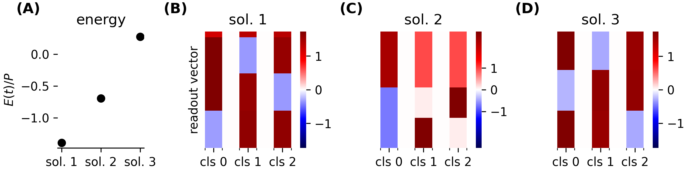
Multiple self-consistent solutions: The energy corresponding to the order parameters can also posses multiple minima, corresponding to different coding schemes. Taking for simplicity such that , the relative probability of two solutions is . We did not observe degeneracy of such that the sampled coding scheme is unique. We show multiple solutions in Fig. 13 on the toy task.
Weight space dynamics: Starting from an initial condition sampled from the prior, both Langevin dynamics and gradient descent first minimize the error and bring the network close to the solution space, as in lazy networks [68]. Already during this early stage a coding scheme emerges. Subsequently, the Langevin dynamics stay close to the solution space and are dominated by the regularization imposed by the prior, which further shapes the coding scheme and eventually leads to the coding scheme shown in (Fig. 4(B)). Interestingly, also gradient descent without noise can arrive at the same solution (see supplement).
B.2 Test Posterior
As in the linear case, we change variables from the weights to the matrix of training and test preactivations . Repeating the steps for the linear network leads to
| (107) |
| (108) |
with the single neuron posteriors
| (109) |
| (110) |
By the same arguments as in the linear case, the saddle-point equations for the train-test and test-test conjugate kernels are for . For , , the saddle-point equations remain identical to the training case.
The saddle-point equations for the kernels are , . At , the conditional distribution of the test preactivations given the training preactivations is identical to the prior distribution in all layers:
| (111) |
where denotes the pseudo inverse. The saddle-point equations for the training kernels remain unchanged. For the train-test and the test-test kernels, the saddle-point equations at are
| (112) |
| (113) |
and , . In the last layer, the conditional distribution of the test preactivations given the training preactivations is also identical to the prior and thus . In total, we arrive at
| (114) |
for the test posterior.
The mean predictor follows immediately from the definition of the joint posterior,
| (115) |
where denotes the preactivation corresponding to the input . For the Gaussian expectation is solvable [69], leading to
| (116) |
where we made the dependence of and on the input explicit. Thus, the mean predictor is
| (117) |
The mean kernels for a pair of inputs also follow immediately from the posterior,
| (118) |
| (119) |
where denote the preactivations corresponding to the inputs . The preactivation kernels are
| (120) |
with .
For the Gaussian expectation can be solved in terms of Owen’s T function [69, 70]; for simplicity we assume for . This decouples the fluctuations of , leading to for .
Summary: Test preactivation posterior on test inputs (121) with (122) (123) and , , . Predictor on single test input : (124) where are the preactivations on . For : with .
Regime : For , the first layer preactivations are restricted to a dimensional subspace and the kernel is singular. The pseudo-inverse appearing in the theory restricts the matrix inversion to the corresponding subspace. To demonstrate that the theory is correct beyond we randomly project the images to a dimensional subspace such that for (see Fig. 22). The nature of the solution indeed stays the same, a redundant code with neurons coding for either one or two classes, and the theory is in accurate quantitative agreement.
Appendix C ReLU Networks ()
C.1 Training & Test Posterior
We directly start with the joint posterior on training and test data but restrict the theory to and set . Following the same initial steps as for the linear and sigmoidal networks leads for the joint posterior of the readout weight matrix and the preactivation matrix on test inputs to
| (125) |
| (126) |
| (127) |
where we dropped the layer index. We explicitly break permutation symmetry for outlier neurons, leading to
| (128) |
| (129) |
Rescaling and for ensures that the contribution from the outliers to the energy is not suppressed by . The corresponding integrals can be solved in saddle-point approximation,
| (130) |
where we used the homogeneity of ReLU, , with saddle-point equations
| (131) |
where denotes a diagonal matrix with elements . The saddle point approximation of the integral leads to
| (132) |
The readout posterior of the bulk neurons concentrates, similar to the sigmoidal case, leading to
| (133) |
Due to the rescaling with all posteriors of the outlier neurons concentrate, leading to
| (134) |
with . The saddle point equation for simplifies to
| (135) |
where the contribution due to the outliers is because both readout weight and preactivation are .
The predictor on a test input is
| (136) |
with . The Gaussian expectation can be solved,
| (137) |
with and .
The kernel on a pair of test inputs is
| (138) |
where denotes the preactivation on the test inputs.
Summary (): Posterior distribution on a set of test inputs separates into bulk neurons where (139) (140) (141) with and outlier neurons where (142) (143) (144) with and ; is determined by . Finally, , , , and . Predictor on test input : (145)
Dynamics: The Langevin dynamics are similar to the dynamics of the sigmoidal networks: first, the loss decreases rapidly which brings the network close to the solution space. Already at this early stage a coding scheme is visible which is, however, not yet sparse. Subsequently, the dynamics is dominated by the regularizer. In this phase sparsity increases over time until the solution with three outliers is reached. In contrast to the sigmoidal case, gradient descent without noise does not reach this maximally sparse solution.
Appendix D Numerics
The code will be made available upon publication on GitHub.
D.1 Empirical Sampling
For all experiments we relied heavily on NumPy [71] and SciPy [72]. To obtain samples from the weight posterior we use Hamiltonian Monte Carlo with the no-u-turn sampler (see, e.g., [73, 74]) implemented in numpyro [75, 76] with jax [77] as a back-end; the model itself is implemented using the front-end provided by pymc [78]. Unless specified otherwise, in all sampling experiments we use a small but finite temperature and keep for . For all experiments, we preprocess each input by subtracting the mean and normalizing such that for all .
D.2 Theory
For linear networks, the solution is straightforward to implement. For nonlinear networks, we solve the saddle point equations by constructing an auxiliary squared loss function with its global minima at the self consistent solutions, e.g., for . This auxiliary loss is minimized using the gradient based minimizer available in jaxopt.ScipyMinimize [79]; after convergence it is checked that the solution achieves zero auxiliary loss, i.e., that a self-consistent solution is obtained.
On the toy example, the minimization is performed jointly for all and ; the one dimensional integrals are solved numerically using Gauss-Hermite quadrature with fixed order for sigmoidal networks or analytical solutions for ReLU networks.
Beyond the toy example, the minimization is performed jointly for all , , and . For ReLU networks, we approximate with to make the auxiliary loss differentiable.
D.3 GP Theory
In the GP theory [12, 13, 14, 15] the predictor mean and variance are
| (146) |
| (147) |
such that the generalization error is where, unlike in non-lazy networks, the second contribution due to the variance cannot be neglected. The associated GP kernel is determined recursively for arbitrary inputs by where are zero mean Gaussian with covariance and . In the predictor the last layer kernel appears, , and denotes the associated matrix on the training inputs , the -dimensional vector containing , and .
Appendix E Supplemental Figures
Brief summary and discussion of the supplemental figures (since we include both pre- and postactivations, we here refer to the latter as postactivations instead of activations):
- •
- •
-
•
Fig. 13: Multiple self-consistent theoretical solutions for the setup from Fig. 4. Each solution corresponds to a saddle point of the integral. Comparing shows that the sampled solution in Fig. 4 has the lowest energy (A). The lowest energy solution does not correspond to the minimal number of codes needed to solve the task: the lowest energy solution comprises 4 codes (B); the other solutions comprise only 3 codes (C,D).
-
•
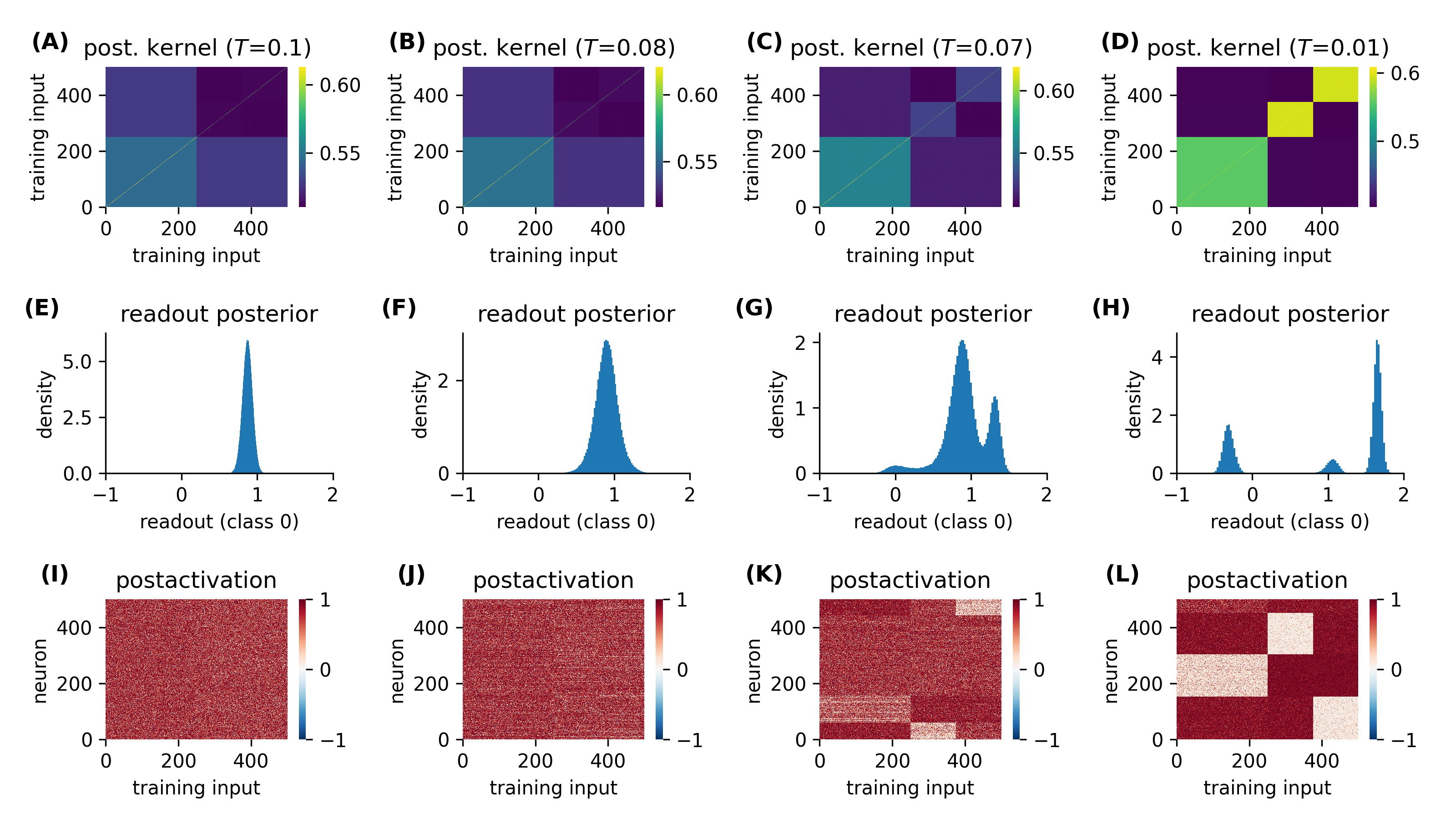
Fig. 14: Temperature dependent phase transition of the coding scheme from Fig. 4. At a high (rescaled) temperature the activations do not exhibit a code and the readout weight posterior is unimodal (A,E,I). At a lower temperature, a coding scheme emerges: is still above the critical temperature (B,F,J) but at a coding scheme emerges involving a subset of the neurons and the readout weight posterior becomes multimodal (C,G,K). Further lowering the temperature to leads to the solution identical to the one shown in Fig. 4 at .
-
•
Fig. 15: Approach to equilibrium using Langevin dynamics for the setup from Fig. 4. Starting from initial conditions sampled from the prior, the Langevin dynamics first rapidly decrease the loss (A; note the logarithmic x-axis) until the solution space is approximately reached. Afterwards, the dynamics decrease the regularizer imposed by the prior while staying at the solution space (B) until the final redundant coding scheme is reached (C,F). After the first phase of approaching the solution space, a coding scheme starts to emerge (D). During the minimization of the regularizer the coding scheme is sharpened (E) until it reaches the final solution (F).
-
•
Fig. 16: Gradient ascent on the log posterior for the setup from Fig. 4, i.e., identical to Fig. 15 except that the dynamics are noiseless. The dynamics go through the same phases of loss minimization (A) and minimization of the regularizer at the solution space (B). The coding scheme is identical to the Langevin case except for missing variability due to the missing noise (C,F). This, however, is dependent on the random initialization; for other random initializations there can be a few neurons with a deviating code (not shown). Similar to Langevin dynamics a code appears after the first phase of approaching the solution space and is further sharpened during the minimization of the regularizer (D,E,F).
- •
-
•
Fig. 18: Approach to equilibrium using Langevin dynamics for the setup from Fig. 8. Similar to the sigmoidal case, the dynamics go through the phases of loss minimization (A) and minimization of the regularizer at the solution space (B) until the final sparse code is reached (C,F). After the first phase of approaching the solution space, a coding scheme starts to emerge which is not yet sparse (D). During the minimization of the regularizer the coding scheme becomes sparser (E) until it reaches the final solution (F).
-
•
Fig. 19: Gradient ascent on the log posterior for the setup from Fig. 8, i.e., identical to Fig. 18 except that the dynamics are noiseless. The dynamics go through the same phases of loss minimization (A) and minimization of the regularizer at the solution space (B). However, unlike in the sigmoidal case, the final solution is different from the Langevin case (C,F). This holds for all tested random initializations. Similar to Langevin dynamics a coding scheme involving all neurons appears after the first phase of approaching the solution space and is further sharpened during the minimization of the regularizer (D,E,F). However, the final solution is less sparse than the solution based on Langevin dynamics. This is likely due to local minima (A) which cannot be overcome without noise.
- •
-
•
Fig. 21: Extended view of the results presented in Fig. 7 including the training preactivations (C), training preactivations of neurons with 0-0-1 code (D), the training preactivation kernel from sampling (E) and theory (F), and the test postactivation kernel from sampling (G) and theory (H). Note that the variability of the preactivations across inputs (C,D) is not apparent in the postactivations (Fig. 7(B)) since the preactivations saturate the sigmoidal nonlinearity; correspondingly the preactivation kernel exhibits more structure (E,F).
- •
-
•
Fig. 23: Application of the theory to three categories of gray scaled CIFAR10 instead of MNIST. Identical to Fig. 21 except for the replacement of MNIST by gray scaled CIFAR10 inputs. While the coding scheme on training data is identical for CIFAR10 (B,C) and MNIST (Fig. 21(B,C)), the test kernels are drastically different and exhibit no structure corresponding to the task (G,H) and the predictor is almost random (I), leading to a high generalization error (A). Put differently, the solution fits the training data but does not generalize.
- •
-
•
Fig. 25: layer sigmoidal network with neurons on all classes of CIFAR10 using the full size of the training data set. The last layer postactivations display a clear coding of the task on the training inputs. These representations generalize to varying extend to test inputs, leading to an overall accuracy of on the full validation set.
-
•
Fig. 26: Extended view of the results presented in Fig. 10 including the training preactivations (C), the training preactivation kernel from sampling (E) and theory (F), and the test postactivation kernel from sampling (G) and theory (H). Note that the preactivations are negative on inputs belonging to classes that the neuron does not code (C), leading to zero postactivations on those inputs.