A locking-free isogeometric thin shell formulation based on higher order accurate local strain projection via approximate dual splines

Abstract

[Abstract]We present a novel isogeometric discretization approach for the Kirchhoff-Love shell formulation based on the Hellinger-Reissner variational principle. For mitigating membrane locking, we discretize the independent strains with spline basis functions that are one degree lower than those used for the displacements. To enable computationally efficient condensation of the independent strains, we first discretize the variations of the independent strains with approximate dual splines to obtain a projection matrix that is close to a diagonal matrix. We then diagonalize this strain projection matrix via row-sum lumping. The combination of approximate dual test functions with row-sum lumping enables the direct condensation of the independent strain fields at the quadrature point level, while maintaining higher-order accuracy at optimal rates of convergence. We illustrate the numerical properties and the performance of our approach through numerical benchmarks, including a curved Euler-Bernoulli beam and the examples of the shell obstacle course.

1 Introduction

Isogeometric analysis (IGA), first introduced by Hughes et al. ¹ in 2005, is a framework that improves the integration of computer-aided design (CAD) and finite element analysis (FEA). The fundamental idea is to employ the same higher-order smooth spline basis functions for both the geometry representation in CAD and the approximation of the field solutions in FEA ². Another benefit of IGA is that it can be directly applied for the discretization of variational formulations that require higher-order smoothness. A salient example is Kirchhoff-Love shell theory, whose Galerkin formulation requires $C^{1}$-continuity of the trial and test functions. A major challenge for finite element schemes that discretize formulations of thin structures such as shells is numerical locking. Primary locking phenomena are membrane and transverse shear locking in beam, plate, and shell elements ^{3, 4, 5} and volumetric locking due to incompressibility in solid elements ⁶. Membrane and transverse shear locking are due to artificial bending stiffness that arises as a result of the coupling of the bending response with the membrane response and transverse shear response, respectively, in the structural model. Locking phenomena negatively affect accuracy and convergence, see e.g. ^{4, 5, 7, 8, 9}.

Locking-preventing discretization technology has been developed for more than 50 years, first within classical FEA and then also within IGA. For the former, prominent locking-preventing approaches are strain modification methods such as the B-bar method ^{10, 11, 12, 13}, the assumed natural strain (ANS) method ^{14, 15, 16}, and the enhanced assumed strain (EAS) method ^{17, 18, 19}; the reduced and selective reduced integration techniques ^{20, 21, 22, 23}, often combined with hourglass control ^{24, 25, 26}; and the utilization of mixed formulations, often based on the Hu-Washizu variational principle ^{21, 22, 27, 28} or the Hellinger-Reissner variational principle ^{18, 29, 30}. Moreover, the effect of locking phenomena can be reduced by increasing the polynomial degree of the basis functions ^{31, 32}, which, however, does not completely eliminate locking, see e.g. ^{8, 32}. In the context of IGA, these approaches have been transferred and extended, for instance, for rod elements ³³, beam elements ^{7, 34, 35, 36, 37}, plate elements ^{36, 38, 39, 40}, shell elements ^{36, 40, 41, 42, 43, 44, 45, 46, 47, 48, 49}, and solid elements ^{38, 50, 51, 52}. For isogeometric discretizations, there exist other reduced quadrature rules that require a minimal number of quadrature points while preserving accuracy and optimal convergence ^{53, 54}. In ^{55, 56}, the authors employed a specific quadrature rule based on the Greville abscissa to alleviate membrane and shear locking for Reissner-Mindlin and Kirchhoff-Love shell elements. Recently, Casquero and co-workers introduced the so-called CAS element based on an assumed-strain approach for quadratic spline functions, where they interpolate the strain fields corresponding to locking with linear Lagrange polynomials. The CAS element idea has been applied for removing membrane and shear locking in linear rod formulations ^{57, 58}, membrane locking in linear Kirchhoff-Love shell formulations ⁵⁹, and volumetric locking in nearly-incompressible linear elasticity ⁶⁰. For Reissner-Mindlin shell formulations based on the Hellinger-Reissner principle, Zou and co-workers ⁶¹ introduced an efficient technique to condense out the strain variables in the mixed formulation. To this end, they suggested to employ the Bézier dual spline basis ^{62, 63}, such that the condensation does not require any matrix inversion. Closely related to this local strain condensation approach are the mixed isogeometric solid-shell element that was introduced by Bouclier and co-workers ⁵⁰, which employs a local quasi-interpolation of the strain variables and enables local strain condensation without matrix inversion; and the blended mixed formulation by Greco and co-workers ^{33, 44} that is based on a local $L^{2}$ projection of the strain variables ⁶⁴.

In this work, inspired by the strain projection technique introduced in ⁶¹, we propose a locking-free isogeometric mixed formulation for Kirchhoff-Love shells based on the Hellinger-Reissner principle. It consists of the following key components. First, to eliminate membrane locking, we follow the widely used idea to discretize the independent strain fields with B-splines of one degree lower than those used for the displacements ^{7, 8, 42}. We choose the multivariate spline spaces for each independent strain component based on those discussed in ⁶⁵. Second, to condense out the independent strain fields, we employ the higher-order diagonalization technique that was applied in ^{66, 67} for mass lumping in explicit dynamics. In particular, we discretize all trial functions and variations of the displacement field with smooth B-splines, but discretize the variations of the independent strain fields with the corresponding modified approximate dual functions ^{66, 67}. Row-sum lumping of the projection matrix yields a diagonal matrix, eliminating the need for matrix inversion while preserving higher-order accuracy and optimal convergence. The strain projection can be performed locally at the quadrature point level, such that the independent strain fields can be condensed out and a purely displacement-based system matrix can be established. We note that similar to the projection technique introduced in ⁶¹, we discretize the trial functions and variations of the independent strain fields with different function spaces and hence obtain a Petrov-Galerkin formulation for the strain projection.

The structure of our article is as follows: in Section 2, we briefly review some of the properties and the construction of the approximate dual functions employed in this work. In Section 3, we briefly review the kinematics of the Kirchhoff-Love shell model. In Section 4, we review the mixed variational formulation of the Kirchhoff-Love shell problem based on the Hellinger-Reissner principle in a continuous setting. We then discretize the independent strain and displacement fields in Section 5 and recall the resulting matrix equations. In Section 6, we specify our approach to obtain a fast and robust local strain projection, using approximate dual functions and row-sum lumping. In Section 7, we present numerical benchmarks of beam and shell problems, demonstrating via spectral analysis and convergence studies that our approach eliminates membrane locking and achieves higher-order accuracy and convergence. In Section 8, we summarize our results and draw conclusions.

2 Approximate dual spline basis

In this section, we review some of the construction and key properties of approximate dual spline functions introduced in ⁶⁸. In addition, we illustrate that employing these approximate dual functions to discretize the test functions in an $L^{2}$ projection preserves the optimal accuracy and convergence, also when the resulting system matrix is diagonalized via row-sum lumping.

2.1 Construction and computation

Splines are piecewise polynomials that are joined smoothly with a prescribed continuity. Spline functions can be represented by B-splines ^{69, 70}. Let $\left\{\right.B_{i},\;i=1,\ldots,N\left.\right\}$ denote a set of B-splines of polynomial degree $p$ defined on an open knot vector that corresponds to a partitioning of the interval $\hat{\Omega}\subset\mathbb{R}$. These functions are a basis for the complete spline space:

$$\mathbb{S}(\hat{\Omega})=\text{span}\left(B_{i},\;i=1,\ldots,N\right).$$ (1)

Let $\langle\cdot,\cdot\rangle$ denote the standard $L^{2}$ inner product on $\hat{\Omega}$. A set of functions $\left\{\right.\bar{B}_{i},\;i=1,\ldots,N\left.\right\}$ is called an $L^{2}$ dual basis (or bi-orthogonal basis) to the set of B-splines if the following property holds:

$$\langle\bar{B}_{i},\,B_{j}\rangle=\delta_{ij},\quad\text{for }i,j\in 1,\ldots,N,$$ (2)

where $\delta_{ij}$ denotes the Kronecker delta. If $\bar{B}_{i}\in\mathbb{S}$, then dual functions are uniquely defined and can be computed using:

$$\bar{B}_{i}(x)=\sum_{j=1}^{N}\left(\mathbf{G}^{-1}\right)_{ij}B_{j}(x),\quad\text{where }G_{ij}=\langle B_{i},\,B_{j}\rangle.$$ (3)

The dual functions are linearly independent and also form a basis for $\mathbb{S}$. However, they are globally supported, which limits their practical usability as test functions.

We loosen the restriction of duality and, instead, search for an alternative basis $\left\{\right.\hat{B}_{i},\;i=1,\ldots,N\left.\right\}$ for the space of splines that achieves duality only in an approximate sense while maintaining local support. Let $\mathbf{S}\in\mathbb{R}^{N\times N}$ denote a symmetric positive definite matrix. We call the set of functions:

$$\hat{B}_{i}(x)=\sum_{j=1}^{N}S_{ij}B_{j}(x),\quad i=1,\ldots,N.$$ (4)

an approximate dual basis to the set of B-splines if:

$$\langle f,\,\hat{B}_{i}\rangle=\langle f,\,\bar{B}_{i}\rangle\quad\forall f\in\mathcal{P}^{p}.$$ (5)

The functions $\left\{\right.\hat{B}_{i},\;i=1,\ldots,N\left.\right\}$ are called approximate dual functions by virtue of (5). They span the space of splines and are linearly independent since $\mathbf{S}$ is invertible.

Notably, the representation is non-unique. A particular useful approximate dual basis has been developed in ⁶⁸. The approximate dual functions presented therein have minimum compact support, in the sense that there exists no other basis that satisfies the approximate duality with smaller supports. This translates into $\mathbf{S}$ having a banded structure with typically $2p+1$ diagonals. Importantly, the matrix $\mathbf{S}$ is an approximate left and right inverse of the Gramian matrix $\mathbf{G}$, that is,

$$\mathbf{S}\approx\mathbf{G}^{-1}.$$ (6)

The matrix is computed by a recursive algorithm, based on fundamental properties of B-splines such as the nestedness of spaces under knot insertion. We refer to the article⁶⁸ for additional details. For application in isogeometric analysis, we refer to ^{66, 67, 71}. In the remainder of this paper, we shall base our construction on this approach.

Remark 2.1.

The approximation (6) can be iteratively improved based on a predictor-multicorrector scheme, see ⁶⁶.

2.2 Geometric mapping

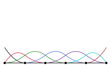
(a) B-splines

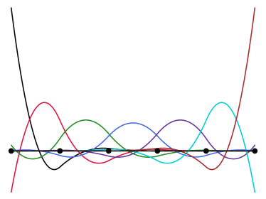
(b) Modified approximate dual functions

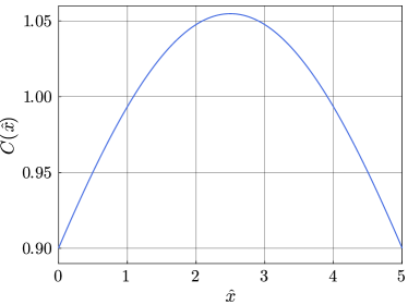
(c) Jacobian determinant function for a quarter circle.

Figure 1: Standard B-splines and modified approximate dual functions for a 1D patch of quadratic B-splines and a non-constant Jacobian determinant (from ⁶⁶).

For general non-affine geometric mappings, the approximation (6), and thus the approximate duality, is not preserved when mapped from the parametric domain $\hat{\Omega}$ to the physical domain $\Omega$. To tackle this problem, we followed ⁷² and introduced in ⁶⁶ a modification of the original approximate dual functions, $\hat{B}_{i}$, by multiplying with the inverse of the determinant of the Jacobian matrix of the mapping, $C(\hat{\mathbf{x}})$. The modified approximate dual functions are:

$$\tilde{B}_{i}(\hat{\boldsymbol{x}})\,:=\,\frac{\hat{B}_{i}(\hat{\boldsymbol{x}})}{C(\hat{\boldsymbol{x}})}\,,\qquad\,i=1,\,\ldots,\,N\,,\quad\hat{\boldsymbol{x}}\in\hat{\Omega}\,.$$ (7)

As shown in ⁶⁶, $\tilde{B}_{i}$ satisfy the approximate duality in the sense of (6) in the physical domain. $\tilde{B}_{i}$ are linearly independent due to the linear independence of the approximate dual functions $\hat{B}_{i}$ and preserve their local support. Their regularity, however, depends on the smoothness of the Jacobian $C(\hat{\boldsymbol{x}})$. For practical scenarios, we can assume that the underlying geometric mapping is assumed to be sufficiently smooth and invertible such that the Jacobian matrix and its inverse are well-defined.

For illustration, we consider a quarter circle with a unit radius represented by a non-uniform rational B-spline (NURBS) curve. In Fig. 1, we plot the modified approximate dual functions (7) next to the corresponding quadratic $C^{1}$-continuous B-splines. We also plot the corresponding non-constant function of the Jacobian determinant. We observe that the modified approximate dual functions have local support and preserve the $C^{p-1}$-continuity of the corresponding B-spline functions.

2.3 $L^{2}$ projection with row-sum lumped matrix

(a) $p=2$

(b) $p=3$

(c) $p=4$

(d) $p=5$

Figure 2: Accuracy and convergence for an $L^{2}$ projection test case (trigonometric function on a quarter circle).

In view of our mixed approach discussed in the following sections, we are interested in the accuracy of the $L^{2}$ projection employing the modified approximate dual functions as test functions when the matrix is diagonalized via row-sum lumping. To this end, we consider the following test problem, which consists of the $L^{2}$ projection of an arbitrary function $f$ onto a space $\mathcal{S}$:
Find $u\in\mathcal{S}$ such that:

$$\langle w,u\rangle=\langle w,f\rangle\,,\quad\forall\,w\in\mathcal{V}\,,$$ (8)

where $u$ denotes the unknown trial function that is the projection of the function $f$, and $w$ denotes the test function. In the case where the two function spaces $\mathcal{S}$ and $\mathcal{V}$ are the same, expression (8) is a Galerkin formulation. When $\mathcal{S}$ and $\mathcal{V}$ are two different function spaces, expression (8) is a Petrov-Galerkin formulation.

We discretize $u$ and $w$ using smooth B-splines of degree $p$ and the corresponding modified approximate dual functions (7), respectively, such that:

$$u^{h}=\sum_{i=1}^{n}\,B_{i}\,\hat{u}^{h}_{i}\,,\qquad w^{h}=\sum_{i=1}^{n}\,\tilde{B}_{i}\,\hat{w}^{h}_{i}\,,$$ (9)

The resulting matrix equation is:

$$\mathbf{M}\,\boldsymbol{\hat{u}}^{h}\,=\,\boldsymbol{F}\,,$$ (10)

where $M_{ij}=\langle\tilde{B}_{i},\,B_{j}\rangle$ and $F_{i}=\langle\tilde{B}_{i},\,f\rangle$. Here, $\boldsymbol{\hat{u}}^{h}$ is the vector of unknown coefficients $\hat{u}^{h}_{i}$, $i=1,\ldots,n$. As shown in ⁶⁷, row-sum lumping of the matrix $\mathbf{M}$ yields the identity matrix due to the definition and construction of the approximate dual functions. Hence, we directly obtain the solution $\boldsymbol{\hat{u}}^{h}\,=\,\boldsymbol{F}$ without any matrix inversion. For explicit dynamics of beam and shell models, the authors showed in ^{66, 67} that when an isogeometric discretization uses the modified approximate dual functions as test functions, employing such a row-sum lumped mass matrix does not compromise higher-order accuracy.

We now illustrate, via the $L^{2}$ projection of the specific function $f(x)=\sin(x)\,\cos(x)$ on a quarter circle exactly represented by a NURBS-curve, that row-sum lumping of the matrix $\mathbf{M}$ does not affect higher-order accuracy and optimal convergence, given that the test functions are discretized with modified approximate dual functions. In Fig. 2, we plot the convergence of the relative $L^{2}$ error in this projection computed with quadratic, cubic, quartic, and quintic discretizations and three different methods: (a) a Galerkin formulation with B-splines as both trial and test functions that uses the inverse of a consistent (black) projection matrix; (b) a Galerkin formulation with B-splines as both trial and test functions that uses the inverse of a row-sum lumped projection matrix (red); and (c) a Petrov-Galerkin formulation with B-splines as trial functions and approximate dual splines as test functions that uses a row-sum lumped projection matrix (blue).

We observe that the Petrov-Galerkin approach with approximate dual test functions leads to results that are several orders of magnitude more accurate than the Galerkin approach using a lumped projection matrix. It achieves the same optimal convergence rate as the reference Galerkin method using the inverse of a consistent projection matrix but at a slightly higher error level. We also see that the accuracy of the projection based on a Galerkin formulation is significantly affected by row-sum lumping, limiting the convergence rate at second order irrespective of the polynomial degree of the spline basis.

3 The Kirchhoff-Love shell model

In this section, we briefly review the Kirchhoff-Love shell model ^{5, 73, 74}, which we employ in this work.

Figure 3: A schematic of shell kinematics.

Consider a shell-like body in $\mathbb{R}^{3}$, illustrated in Fig. 3, that is, locally, described by curvilinear coordinates $\theta=(\theta^{1},\theta^{2},\theta^{3})$. In the following, we adopt the Einstein summation convention and the convention for Greek and Latin letters, i.e. $i=1,2,3$ and $\alpha=1,2$. The reference and current configurations of the shell-like body are described by the position vector $\boldsymbol{X}(\theta)$ and $\boldsymbol{x}(\theta)$, respectively, as follows:

$$\boldsymbol{X}(\theta)=\theta^{\alpha}\boldsymbol{A}_{\alpha}+\theta^{3}\boldsymbol{A}_{3}\,,\qquad\boldsymbol{x}(\theta)=\theta^{\alpha}\boldsymbol{a}_{\alpha}+\theta^{3}\boldsymbol{a}_{3}\,.$$ (11)

The two are related through the deformation:

$$\boldsymbol{u}(\theta)=\boldsymbol{x}(\theta)-\boldsymbol{X}(\theta)\,.$$ (12)

Here, $\theta^{3}$ is the coordinate in the thickness direction $-d/2\leq\theta^{3}\leq d/2$, where $d$ denotes the shell thickness. $\boldsymbol{A}_{i}$ and $\boldsymbol{a}_{i}$ denote the covariant base vectors of the midsurface in the reference configuration and the current configuration, respectively. $\boldsymbol{A}_{i}$ and $\boldsymbol{a}_{i}$ are defined in terms of the position vector of the midsurface $\bar{\boldsymbol{X}}$ and $\bar{\boldsymbol{x}}$ as follows:

$$\boldsymbol{A}_{\alpha}=\bar{\boldsymbol{X}}_{,\alpha}\,,\qquad\boldsymbol{A}_{3}=\frac{\boldsymbol{A}_{1}\times\boldsymbol{A}_{2}}{|\boldsymbol{A}_{1}\times\boldsymbol{A}_{2}|}\,,$$ (13)

$$\boldsymbol{a}_{\alpha}=\bar{\boldsymbol{x}}_{,\alpha}\,,\qquad\boldsymbol{a}_{3}=\frac{\boldsymbol{a}_{1}\times\boldsymbol{a}_{2}}{|\boldsymbol{a}_{1}\times\boldsymbol{a}_{2}|}\,,$$ (14)

where $(\cdot)_{,\alpha}$ denotes $\partial(\cdot)/\partial\theta^{\alpha}$. The covariant base vectors at any point in the shell continuum in the reference and current configurations are:

$$\boldsymbol{G}_{\alpha}=\boldsymbol{X}_{,\alpha}\quad\text{and}\quad\boldsymbol{g}_{\alpha}=\boldsymbol{x}_{,\alpha}\,,$$ (15)

respectively. The corresponding normal vectors are denoted by $\boldsymbol{G}_{3}$ and $\boldsymbol{g}_{3}$, respectively. Contravariant base vectors, $\boldsymbol{G}^{\alpha}$ and $\boldsymbol{g}^{\alpha}$, can be computed directly from the first fundamental form.

The Green-Lagrange strain tensor is defined as $\mathbf{E}=E_{\alpha\beta}\,\boldsymbol{G}^{\alpha}\otimes\boldsymbol{G}^{\beta}$. For Kirchhoff-Love shells, the non-zero strain components $E_{\alpha\beta}$ can be represented by the sum of a constant membrane action and a linearly varying bending action due to the change of curvature:

$$E_{\alpha\beta}=\varepsilon_{\alpha\beta}+\theta^{3}\kappa_{\alpha\beta}.$$ (16)

The coefficients $\varepsilon_{\alpha\beta}$ and $\kappa_{\alpha\beta}$, which can be computed from the first and second fundamental form, see e.g. ^{5, 73, 74}, are:

$$\varepsilon_{\alpha\beta}=\frac{1}{2}\left(\boldsymbol{a}_{\alpha}\cdot\boldsymbol{a}_{\beta}-\boldsymbol{A}_{\alpha}\cdot\boldsymbol{A}_{\beta}\right)\quad\text{and}\quad\kappa_{\alpha\beta}=\boldsymbol{A}_{\alpha,\beta}\cdot\boldsymbol{A}_{3}-\boldsymbol{a}_{\alpha,\beta}\cdot\boldsymbol{a}_{3}\,.$$ (17)

In Voigt notation, the strains due to membrane and bending action are:

$$\boldsymbol{\varepsilon}=\begin{bmatrix}\varepsilon_{11}\\ \varepsilon_{22}\\ 2\varepsilon_{12}\end{bmatrix}\,,\quad\boldsymbol{\kappa}=\begin{bmatrix}\kappa_{11}\\ \kappa_{22}\\ 2\kappa_{12}\end{bmatrix}\,,$$ (18)

respectively. The first variation of the strain components are:

$$\delta\varepsilon_{\alpha\beta}=\frac{1}{2}\left(\delta\boldsymbol{a}_{\alpha}\cdot\boldsymbol{a}_{\beta}+\boldsymbol{a}_{\alpha}\cdot\delta\boldsymbol{a}_{\beta}\right)\,,$$ (19)

$$\delta\kappa_{\alpha\beta}=-\left(\delta\boldsymbol{a}_{\alpha,\beta}\cdot\boldsymbol{a}_{3}+\boldsymbol{a}_{\alpha,\beta}\cdot\delta\boldsymbol{a}_{3}\right)\,,$$ (20)

and the second variation are:

$$\Delta\delta\varepsilon_{\alpha\beta}=\frac{1}{2}\left(\delta\boldsymbol{a}_{\alpha}\cdot\Delta\boldsymbol{a}_{\beta}+\Delta\boldsymbol{a}_{\alpha}\cdot\delta\boldsymbol{a}_{\beta}\right)\,,$$ (21)

$$\Delta\delta\kappa_{\alpha\beta}=-\left(\delta\boldsymbol{a}_{\alpha,\beta}\cdot\Delta\boldsymbol{a}_{3}+\Delta\boldsymbol{a}_{\alpha,\beta}\cdot\delta\boldsymbol{a}_{3}+\boldsymbol{a}_{\alpha,\beta}\cdot\Delta\delta\boldsymbol{a}_{3}\right)\,.$$ (22)

The components of the second Piola Kirchhoff stress resultants $\boldsymbol{n}$ and $\boldsymbol{m}$ (which are energetically conjugate to the Green-Lagrange strains) are:

$$\boldsymbol{n}=d\,\mathbf{C}\;\boldsymbol{\varepsilon}\,,\qquad\boldsymbol{m}=\frac{d^{3}}{12}\mathbf{C}\;\boldsymbol{\kappa}\,,$$ (23)

where $\mathbf{C}$ denotes the material matrix that is:

$$\mathbf{C}=\frac{E}{1-\nu^{2}}\,\begin{bmatrix}1&\nu&0\\ \nu&1&0\\ 0&0&\frac{1-\nu}{2}\end{bmatrix}\,.$$ (24)

where we assume the Saint Venant-Kirchhoff material model, i.e. a linear relationship. Here, $E$ and $\nu$ are the Young’s modulus and Poisson’s ratio. We note that the strains and stress resultants in (23) are defined in a local Cartesian coordinate system.

4 Mixed variational formulation

In this section, we briefly recall the Hu-Washizu and the Hellinger-Reissner variational principles of elastostatics, see e.g. ⁷⁵, which form the starting point for the developments in the remainder of this work.

4.1 The Hu-Washizu principle

We recall the three-field Hu-Washizu functional ^{76, 77, 78}:

$$\Pi_{HW}(\boldsymbol{u},\mathbf{E},\mathbf{S})\;= \;\frac{1}{2}\int_{\Omega}\mathbf{E}^{T}\,(\mathbf{C}\ \mathbf{E})\;\mathrm{d}\Omega-\int_{\Omega}\boldsymbol{u}^{T}\boldsymbol{F}_{b}\;\mathrm{d}\Omega-\int_{\Gamma_{t}}\boldsymbol{u}^{T}\,\boldsymbol{F}_{t}\;\mathrm{d}\Gamma$$

$$-\int_{\Omega}\mathbf{S}^{T}(\mathbf{E}-\mathscr{E}(\boldsymbol{u}))\;\mathrm{d}\Omega-\int_{\Gamma_{u}}(\mathbf{S}\,^{T}\boldsymbol{\nu})\,(\boldsymbol{u}-\boldsymbol{u}_{0})\;\mathrm{d}\Gamma\,,$$ (25)

defined for an elastic body with domain $\Omega$, where we write all strain and stress quantities in Voigt notation.

The variables $\boldsymbol{u}$, $\mathbf{E}$, and $\mathbf{S}$ denote independent displacement, strain, and stress fields, which are also sometimes denoted as master fields in this context ⁷⁵. To distinguish the dependent strain fields from the independent strain fields, we introduce the strain-displacement operator $\mathscr{E}(\boldsymbol{u})$, which acts on the displacement field to produce the dependent strain fields via the kinematic relations. The resulting dependent fields are also sometimes denoted as slave fields in this context ⁷⁵.

Furthermore, $\mathbf{C}$ is the material matrix, relating stresses and strains, $\boldsymbol{F}_{b}$ is the body force acting on the elastic body $\Omega$, $\boldsymbol{F_{t}}$ the traction acting on the traction boundary $\Gamma_{t}$, $\boldsymbol{\nu}$ is a matrix that acts on a stress vector in Voigt notation to produce the traction vector based on the outward-facing unit normal to the displacement boundary $\Gamma_{u}$, and $\boldsymbol{u}_{0}$ the prescribed displacement on $\Gamma_{u}$.

We observe in (4.1) that its last two terms contain the residuals of the kinematic strain-displacement relation and the displacement boundary conditions. The corresponding relations are imposed variationally by multiplication with energetically conjugate stress and traction fields that act as Langrange multipliers.

The Hu-Washizu variational theorem then states that:

$$\Pi_{HW}(\boldsymbol{u},\mathbf{E},\mathbf{S})\;=\;\text{Stationary}\,.$$ (26)

4.2 The Hellinger-Reissner principle

A Hellinger-Reissner functional ^{79, 80} can be derived from the Hu-Washizu functional (4.1) by assuming that the constitutive law and the Dirichlet boundary conditions are strongly satisfied ⁶¹, i.e.:

$$\mathbf{S}=\mathbf{C}\ \mathbf{E}\quad\text{ on }\Omega\,,$$ (27)

$$\boldsymbol{u}=\boldsymbol{u}_{0}\quad\text{ on }\Gamma_{u}\,,$$ (28)

The Hellinger-Reissner functional follows as:

$$\Pi_{HR}(\boldsymbol{u},\mathbf{E})\; =\;\int_{\Omega}\mathbf{E}^{T}\,\left(\mathbf{C}\,\mathscr{E}(\boldsymbol{u})\right)-\frac{1}{2}\,\mathbf{E}^{T}\,(\mathbf{C}\ \mathbf{E})-\boldsymbol{u}^{T}\boldsymbol{F}_{b}\;\mathrm{d}\Omega-\int_{\Gamma_{t}}\boldsymbol{u}^{T}\,\boldsymbol{F}_{t}\;\mathrm{d}\Gamma\,.$$ (29)

Our $\Pi_{HR}(\boldsymbol{u},\mathbf{E})$ is also known as the modified Hellinger-Reissner functional, since it considers the strains, instead of the stresses, as the independent master field ⁶¹. We note that to distinguish the dependent strain field derived from the displacements, we again use the strain-displacement operator $\mathscr{E}(\boldsymbol{u})$, which acts on the displacement field to produce the dependent strain fields.

The Hellinger-Reissner variational theorem states that:

$$\Pi_{HR}(\boldsymbol{u},\mathbf{E})\;=\;\text{Stationary}\,,$$ (30)

i.e. the variation of the Hellinger-Reissner functional equals zero, that is:

$$\delta\Pi_{HR}(\boldsymbol{u},\delta\boldsymbol{u},\mathbf{E},\delta\mathbf{E})=\int_{\Omega}\delta\mathscr{E}(\boldsymbol{u})^{T}\,(\mathbf{C}\ \mathbf{E})+\delta\mathbf{E}^{T}\,\left[\mathbf{C}\,\left(\mathscr{E}(\boldsymbol{u})-\mathbf{E}\right)\right]\;\mathrm{d}\Omega-\int_{\Omega}\delta\boldsymbol{u}^{T}\,\boldsymbol{F}_{b}\;\mathrm{d}\Omega-\int_{\Gamma_{t}}\delta\boldsymbol{u}^{T}\,\boldsymbol{F}_{t}\;\mathrm{d}\Gamma=0\,.$$ (31)

These nonlinear equations must be solved via linearization and the Newton-Raphson method. The linearization yields ⁶¹:

$$L\left[\delta\Pi_{HR}(\boldsymbol{u},\delta\boldsymbol{u},\mathbf{E},\delta\mathbf{E})\right]=\delta\Pi_{HR}(\boldsymbol{u},\delta\boldsymbol{u},\mathbf{E},\delta\mathbf{E})+\Delta\delta\Pi_{HR}(\Delta\boldsymbol{u},\delta\boldsymbol{u},\Delta\mathbf{E},\delta\mathbf{E})=0\,,$$ (32)

where

$$\Delta\delta\Pi_{HR}(\Delta\boldsymbol{u},\delta\boldsymbol{u},\Delta\mathbf{E},\delta\mathbf{E}) =\underbrace{\int_{\Omega}-\delta\mathbf{E}^{T}\,\left(\mathbf{C}\,\Delta\mathbf{E}\right)+\delta\mathbf{E}^{T}\,\left[\mathbf{C}\,\Delta\mathscr{E}(\boldsymbol{u})\right]+\delta\mathscr{E}(\boldsymbol{u})^{T}\,\left(\mathbf{C}\,\Delta\mathbf{E}\right)\;\mathrm{d}\Omega}_{\text{material stiffness}}$$

$$+\underbrace{\int_{\Omega}\Delta\delta\mathscr{E}(\boldsymbol{u})^{T}\,(\mathbf{C}\ \mathbf{E})+\Delta\delta\mathbf{E}^{T}\,\left[\mathbf{C}\,\left(\mathscr{E}(\boldsymbol{u})-\mathbf{E}\right)\right]\;\mathrm{d}\Omega}_{\text{geometric stiffness}}$$ (33)

4.3 Weak formulation of Kirchhoff-Love shells in mixed format

We now cast the Kirchhoff shell formulation reviewed in the previous section into Hellinger-Reissner format. To this end, we consider the membrane and bending strains as independent master fields. We now distinguish between the independent strain field

$$\mathbf{E}=\boldsymbol{e}+\theta^{3}\,\boldsymbol{k}\,.$$ (34)

which consists of the independent membrane and bending strain fields, $\boldsymbol{e}$ and $\boldsymbol{k}$, and the strain-displacement operator

$$\mathscr{E}(\boldsymbol{u})=\boldsymbol{\varepsilon}+\theta^{3}\,\boldsymbol{\kappa}\,.$$ (35)

which consists of the displacement-dependent membrane and bending fields $\boldsymbol{\varepsilon}$ and $\boldsymbol{\kappa}$. We note that the latter are strongly related to the displacements via the shell kinematics reviewed in (11) to (22).

We now substitute (34) and (35) (in Voigt notation) into the Hellinger-Reissner variational formulation (29), use the material matrix (24) and analytically integrate through the thickness. We then obtain the following mixed variational formulation of the Kirchhoff-Love shell problem:

$$d\int_{\bar{\Omega}}\delta\boldsymbol{e}^{T}\mathbf{C}\left(\boldsymbol{\varepsilon}-\boldsymbol{e}\right)+\delta\boldsymbol{\varepsilon}^{T}\mathbf{C}\,\boldsymbol{e}\;\mathrm{d}\bar{\Omega}\,+\,\frac{d^{3}}{12}\int_{\bar{\Omega}}\delta\boldsymbol{k}^{T}\mathbf{C}\left(\boldsymbol{\kappa}-\boldsymbol{k}\right)+\delta\boldsymbol{\kappa}^{T}\mathbf{C}\,\boldsymbol{k}\;\mathrm{d}\bar{\Omega}-d\int_{\bar{\Omega}}\,\delta\boldsymbol{u}^{T}\,\boldsymbol{F}_{b}\;\mathrm{d}\bar{\Omega}-d\int_{\bar{\Gamma}_{t}}\,\delta\boldsymbol{u}^{T}\boldsymbol{F}_{t}\;\mathrm{d}\bar{\Gamma}\,=0\,,$$ (36)

where $\bar{\Omega}$ and $\bar{\Gamma}_{t}$ denote the middle surface of the shell body and its traction boundary, respectively.

Remark 4.1.

In (36), we assume that the shell is subjected merely to the body force $\boldsymbol{F}_{b}$ and the traction $\boldsymbol{F}_{t}$ at the traction boundary (see e.g. ⁶⁵). For ease of notation, we neglect here other Neumann boundary conditions, for instance, due to bending moments. The Dirichlet boundary conditions are enforced strongly via prescribing the displacement of the corresponding control points, see e.g. ⁷³.

Taking into account the independence of the variations of the different fields, we can write this equation in the following three separate variational statements:

$$d\int_{\bar{\Omega}}\delta\boldsymbol{\varepsilon}^{T}\mathbf{C}\,\boldsymbol{e}\;\mathrm{d}\bar{\Omega}+\frac{d^{3}}{12}\int_{\bar{\Omega}}\delta\boldsymbol{\kappa}^{T}\mathbf{C}\,\boldsymbol{k}\;\mathrm{d}\bar{\Omega}\; =\;d\int_{\bar{\Omega}}\,\delta\boldsymbol{u}^{T}\,\boldsymbol{F}_{b}\;\mathrm{d}\bar{\Omega}+d\int_{\bar{\Gamma}_{t}}\,\delta\boldsymbol{u}^{T}\boldsymbol{F}_{t}\;\mathrm{d}\bar{\Gamma}$$ (37a)

$$d\int_{\bar{\Omega}}\delta\boldsymbol{e}^{T}\mathbf{C}\left(\boldsymbol{\varepsilon}-\boldsymbol{e}\right)\;\mathrm{d}\bar{\Omega}\; =\;0$$ (37b)

$$\frac{d^{3}}{12}\int_{\bar{\Omega}}\delta\boldsymbol{k}^{T}\mathbf{C}\left(\boldsymbol{\kappa}-\boldsymbol{k}\right)\;\mathrm{d}\bar{\Omega}\; =\;0\,.$$ (37c)

It is straightforward to identify the last two equations in (38) as the projection of the displacement-dependent membrane and bending strain fields, $\boldsymbol{\varepsilon}$ and $\boldsymbol{\kappa}$, on the independent membrane and bending strain fields, such that the remaining difference between the corresponding fields is minimized with respect to the strain energy norm. The last two equations of the system (38) are therefore equivalent to the projection (8), with the exception of the two different norms.

Following (32), we can write the linearization of the system (38) as follows:

$$d\, \int_{\bar{\Omega}}\Delta\delta\boldsymbol{\varepsilon}^{T}\mathbf{C}\,\boldsymbol{e}\;\mathrm{d}\bar{\Omega}+\frac{d^{3}}{12}\,\int_{\bar{\Omega}}\Delta\delta\boldsymbol{\kappa}^{T}\mathbf{C}\,\boldsymbol{k}\;\mathrm{d}\bar{\Omega}\,+\,d\,\int_{\bar{\Omega}}\delta\boldsymbol{\varepsilon}^{T}\mathbf{C}\,\Delta\boldsymbol{e}\;\mathrm{d}\bar{\Omega}\,+\,\frac{d^{3}}{12}\int_{\bar{\Omega}}\delta\boldsymbol{\kappa}^{T}\mathbf{C}\,\Delta\boldsymbol{k}\;\mathrm{d}\bar{\Omega}$$

$$\qquad\qquad=d\,\int_{\bar{\Omega}}\,\delta\boldsymbol{u}^{T}\,\boldsymbol{F}_{b}\;\mathrm{d}\bar{\Omega}+d\,\int_{\bar{\Gamma}_{t}}\,\delta\boldsymbol{u}^{T}\boldsymbol{F}_{t}\;\mathrm{d}\bar{\Gamma}-d\,\int_{\bar{\Omega}}\delta\boldsymbol{\varepsilon}^{T}\mathbf{C}\,\boldsymbol{e}\;\mathrm{d}\bar{\Omega}-\frac{d^{3}}{12}\int_{\bar{\Omega}}\delta\boldsymbol{\kappa}^{T}\mathbf{C}\,\boldsymbol{k}\;\mathrm{d}\bar{\Omega}$$ (38a)

$$d\, \int_{\bar{\Omega}}\delta\boldsymbol{e}^{T}\mathbf{C}\,\Delta\boldsymbol{\varepsilon}-\delta\boldsymbol{e}^{T}\mathbf{C}\,\Delta\boldsymbol{e}\;\mathrm{d}\bar{\Omega}\,=\,-d\,\int_{\bar{\Omega}}\delta\boldsymbol{e}^{T}\mathbf{C}\left(\boldsymbol{\varepsilon}-\boldsymbol{e}\right)\;\mathrm{d}\bar{\Omega}$$ (38b)

$$\frac{d^{3}}{12}\, \int_{\bar{\Omega}}\delta\boldsymbol{k}^{T}\mathbf{C}\,\Delta\boldsymbol{\kappa}-\delta\boldsymbol{k}^{T}\mathbf{C}\,\Delta\boldsymbol{k}\;\mathrm{d}\bar{\Omega}\,=\,-\frac{d^{3}}{12}\int_{\bar{\Omega}}\delta\boldsymbol{k}^{T}\mathbf{C}\left(\boldsymbol{\kappa}-\boldsymbol{k}\right)\;\mathrm{d}\bar{\Omega}\,.$$ (38c)

which is the starting point to set up a Newton-Raphson procedure in a straightforward way.

Remark 4.2.

For Kirchhoff-Love shells, where only membrane locking occurs, we note that an alternative is to merely consider the membrane strains, $\boldsymbol{e}$, as unknown auxiliary variables ⁶⁵. This is equivalent to assuming $\boldsymbol{k}=\boldsymbol{\kappa}$ for all points in $\Omega$. Equation (36) then becomes:

$$d\int_{\bar{\Omega}}\delta\boldsymbol{e}^{T}\mathbf{C}\left(\boldsymbol{\varepsilon}-\boldsymbol{e}\right)+\delta\boldsymbol{\varepsilon}^{T}\mathbf{C}\,\boldsymbol{e}\;\mathrm{d}\bar{\Omega}\,+\,\frac{d^{3}}{12}\int_{\bar{\Omega}}\delta\boldsymbol{\kappa}^{T}\mathbf{C}\,\boldsymbol{\kappa}\;\mathrm{d}\bar{\Omega}-d\int_{\bar{\Omega}}\,\delta\boldsymbol{u}^{T}\,\boldsymbol{F}_{b}\;\mathrm{d}\bar{\Omega}-d\int_{\bar{\Gamma}_{t}}\,\delta\boldsymbol{u}^{T}\boldsymbol{F}_{t}\;\mathrm{d}\bar{\Gamma}\,=0\,,$$ (39)

which can be again expressed in the following separate variational statements:

$$d\int_{\bar{\Omega}}\delta\boldsymbol{\varepsilon}^{T}\mathbf{C}\,\boldsymbol{e}\;\mathrm{d}\bar{\Omega}+\frac{d^{3}}{12}\int_{\bar{\Omega}}\delta\boldsymbol{\kappa}^{T}\mathbf{C}\,\boldsymbol{\kappa}\;\mathrm{d}\bar{\Omega}\; =\;d\int_{\bar{\Omega}}\,\delta\boldsymbol{u}^{T}\,\boldsymbol{F}_{b}\;\mathrm{d}\bar{\Omega}+d\int_{\bar{\Gamma}_{t}}\,\delta\boldsymbol{u}^{T}\boldsymbol{F}_{t}\;\mathrm{d}\bar{\Gamma}$$ (40a)

$$d\int_{\bar{\Omega}}\delta\boldsymbol{e}^{T}\mathbf{C}\left(\boldsymbol{\varepsilon}-\boldsymbol{e}\right)\;\mathrm{d}\bar{\Omega}\; =\;0\,.$$ (40b)

We note that this is no longer a second-order problem as in the case of (36), but a fourth-order problem.

5 Isogeometric discretization and matrix formulation

To eliminate membrane locking in the Kirchhoff-Love shell formulation, we follow the well-established strategy of discretizing the independent strains with spline basis functions that are one degree lower than those used for the displacements ^{7, 8, 42, 65}. Following the discrete spline spaces chosen in Guo and co-workers ⁶⁵, we discretize the the displacement vector $\boldsymbol{u}$, the membrane strains $\boldsymbol{e}$, and the bending strains $\boldsymbol{k}$ as follows:

$$\boldsymbol{u}^{h}=\begin{bmatrix}u_{1}^{h}\\ u_{2}^{h}\\ u_{3}^{h}\end{bmatrix}=\sum_{i=1}^{n}\,\begin{bmatrix}B_{i}^{p,p}\,\hat{u}_{1,i}^{h}\\ B_{i}^{p,p}\,\hat{u}_{2,i}^{h}\\ B_{i}^{p,p}\,\hat{u}_{3,i}^{h}\end{bmatrix}=\sum_{i=1}^{n}\,B_{i}^{p,p}\mathbf{I}\,\begin{bmatrix}\hat{u}_{1,i}^{h}\\ \hat{u}_{2,i}^{h}\\ \hat{u}_{3,i}^{h}\end{bmatrix}=\sum_{i=1}^{n}\,\mathbf{B}_{i}\,\boldsymbol{\hat{u}}_{i}^{h}\,,$$ (41)

$$\boldsymbol{e}^{h}=\begin{bmatrix}e_{11}^{h}\\ e_{22}^{h}\\ 2e_{12}^{h}\end{bmatrix}=\sum_{i=1}^{m}\,\begin{bmatrix}N_{i}^{p-1,p}\,\hat{e}_{11,i}^{h}\\ N_{i}^{p,p-1}\,\hat{e}_{22,i}^{h}\\ N_{i}^{p-1,p-1}\,2\hat{e}_{12,i}^{h}\end{bmatrix}=\sum_{i=1}^{m}\,\begin{bmatrix}N_{i}^{p-1,p}&0&0\\ 0&N_{i}^{p,p-1}&0\\ 0&0&N_{i}^{p-1,p-1}\end{bmatrix}\,\begin{bmatrix}\hat{e}_{11,i}^{h}\\ \hat{e}_{22,i}^{h}\\ 2\hat{e}_{12,i}^{h}\end{bmatrix}=\sum_{i=1}^{m}\,\mathbf{N}_{i}\,\boldsymbol{\hat{e}}_{i}^{h}\,.$$ (42)

$$\boldsymbol{k}^{h}=\begin{bmatrix}k_{11}^{h}\\ k_{22}^{h}\\ 2k_{12}^{h}\end{bmatrix}=\sum_{i=1}^{m}\,\begin{bmatrix}N_{i}^{p-1,p}\,\hat{k}_{11,i}^{h}\\ N_{i}^{p,p-1}\,\hat{k}_{22,i}^{h}\\ N_{i}^{p-1,p-1}\,2\hat{k}_{12,i}^{h}\end{bmatrix}=\sum_{i=1}^{m}\,\begin{bmatrix}N_{i}^{p-1,p}&0&0\\ 0&N_{i}^{p,p-1}&0\\ 0&0&N_{i}^{p-1,p-1}\end{bmatrix}\,\begin{bmatrix}\hat{k}_{11,i}^{h}\\ \hat{k}_{22,i}^{h}\\ 2\hat{k}_{12,i}^{h}\end{bmatrix}=\sum_{i=1}^{m}\,\mathbf{N}_{i}\,\boldsymbol{\hat{k}}_{i}^{h}\,.$$ (43)

Here, the basis $B_{i}^{p,p}$, $i=1,\ldots,n$, consists of spline basis functions of degree $p$ in both $\theta^{1}$ and $\theta^{2}$ directions, and the basis $N_{i}^{p-1,p}$, $i=1,\ldots,m$, consists of spline functions of degree $p-1$ and $p$ in $\theta^{1}$ and $\theta^{2}$ directions, respectively. The notation follows analogously for the spline basis $N_{i}^{p,p-1}$ and the spline basis $N_{i}^{p-1,p-1}$. The unknown coefficients can be summarized in subvectors $\boldsymbol{\hat{u}}_{i}^{h}$, $\boldsymbol{\hat{e}}_{i}^{h}$, and $\boldsymbol{\hat{k}}_{i}^{h}$ for each basis function, and later assembled into corresponding global vectors $\boldsymbol{\hat{u}}^{h}$, $\boldsymbol{\hat{e}}^{h}$, and $\boldsymbol{\hat{k}}^{h}$.

One can discretize the variations of the displacements, membrane and bending strains using the same spline spaces of the corresponding independent master field, i.e.:

$$\delta\boldsymbol{u}^{h}=\sum_{i=1}^{n}\,\mathbf{B}_{i}\,\delta\boldsymbol{\hat{u}}^{h}_{i}\,,$$ (44)

$$\delta\boldsymbol{e}^{h}=\sum_{i=1}^{m}\,\mathbf{N}_{i}\,\delta\boldsymbol{\hat{e}}_{i}^{h}\,,$$ (45)

$$\delta\boldsymbol{k}^{h}=\sum_{i=1}^{m}\,\mathbf{N}_{i}\,\delta\boldsymbol{\hat{k}}_{i}^{h}\,,$$ (46)

Inserting the interpolation of the displacements, membrane and bending strains, and their variations, into the linearized equations (38) leads to the following linear system solved in each Newton-Raphson iteration:

$$\begin{bmatrix}\mathbf{K}_{11}^{\text{geom}}&\mathbf{K}_{12}&\mathbf{K}_{13}\\ \mathbf{K}_{21}&\mathbf{K}_{22}&\mathbf{0}\\ \mathbf{K}_{31}&\mathbf{0}&\mathbf{K}_{33}\\ \end{bmatrix}\,\begin{bmatrix}\Delta\boldsymbol{\hat{u}}^{h}\\ \Delta\boldsymbol{\hat{e}}^{h}\\ \Delta\boldsymbol{\hat{k}}^{h}\end{bmatrix}=\begin{bmatrix}\boldsymbol{F}_{ext}-\boldsymbol{F}_{int}\\ -\boldsymbol{F}^{m}_{int}\\ -\boldsymbol{F}^{b}_{int}\end{bmatrix}\,,$$ (47)

where

$$\mathbf{K}_{11}^{\text{geom}}=\int_{\bar{\Omega}}\mathbf{K}_{11}^{\text{m,geom}}\,+\,\mathbf{K}_{11}^{\text{b,geom}}\;\mathrm{d}\bar{\Omega}\,,$$ (48)

$$\mathbf{K}_{12}=d\,\int_{\bar{\Omega}}\left(\mathbf{B}^{m}\right)^{T}\mathbf{C}\,\mathbf{N}\;\mathrm{d}{\bar{\Omega}}\,,$$ (49)

$$\mathbf{K}_{21}=d\,\int_{\bar{\Omega}}\mathbf{N}^{T}\mathbf{C}\,\mathbf{B}^{m}\;\mathrm{d}\bar{\Omega}\,,$$ (50)

$$\mathbf{K}_{22}=-d\,\int_{\bar{\Omega}}\mathbf{N}^{T}\mathbf{C}\,\mathbf{N}\;\mathrm{d}\bar{\Omega}\,,$$ (51)

$$\mathbf{K}_{13}=\frac{d^{3}}{12}\int_{\bar{\Omega}}\left(\mathbf{B}^{b}\right)^{T}\mathbf{C}\,\mathbf{N}\;\mathrm{d}{\bar{\Omega}}\,,$$ (52)

$$\mathbf{K}_{31}=\frac{d^{3}}{12}\int_{\bar{\Omega}}\mathbf{N}^{T}\mathbf{C}\,\mathbf{B}^{b}\;\mathrm{d}\bar{\Omega}\,,$$ (53)

$$\mathbf{K}_{33}=-\frac{d^{3}}{12}\int_{\bar{\Omega}}\mathbf{N}^{T}\mathbf{C}\,\mathbf{N}\;\mathrm{d}\bar{\Omega}\,,$$ (54)

$$\boldsymbol{F}_{int}=d\,\int_{\bar{\Omega}}\left(\mathbf{B}^{m}\right)^{T}\mathbf{C}\,\boldsymbol{e}^{h}\;\mathrm{d}\bar{\Omega}\,+\,\frac{d^{3}}{12}\int_{\bar{\Omega}}\left(\mathbf{B}^{b}\right)^{T}\mathbf{C}\,\boldsymbol{k}^{h}\;\mathrm{d}\bar{\Omega}\,,$$ (55)

$$\boldsymbol{F}^{m}_{int}=d\,\int_{\bar{\Omega}}\mathbf{N}^{T}\mathbf{C}\left(\boldsymbol{\varepsilon}^{h}-\boldsymbol{e}^{h}\right)\;\mathrm{d}\bar{\Omega}\,,$$ (56)

$$\boldsymbol{F}^{b}_{int}=\frac{d^{3}}{12}\int_{\bar{\Omega}}\mathbf{N}^{T}\mathbf{C}\left(\boldsymbol{\kappa}^{h}-\boldsymbol{k}^{h}\right)\;\mathrm{d}\bar{\Omega}\,,$$ (57)

$$\boldsymbol{F}_{ext}=d\,\int_{\bar{\Omega}}\mathbf{B}^{T}\boldsymbol{F}_{b}\;\mathrm{d}\bar{\Omega}\,+\,d\,\int_{\bar{\Gamma}_{t}}\mathbf{B}^{T}\boldsymbol{F}_{t}\;\mathrm{d}\bar{\Gamma}\,.$$ (58)

The quantities $\mathbf{B}^{m}$ and $\mathbf{B}^{b}$ denote the strain-displacement matrices corresponding to the membrane and bending strains, respectively. The matrices $\mathbf{K}_{11}^{\text{m,geom}}$ and $\mathbf{K}_{11}^{\text{b,geom}}$ denote the contributions to the geometric stiffness matrix due to the membrane and bending deformations, respectively. The quantities $\mathbf{N}$ and $\mathbf{B}$ denote the matrices of basis functions for discretizing the strains and the displacements, respectively. For more details, we refer the interested reader to the Appendix A, where we summarize the derivation of these matrices and the force vectors.

Remark 5.1.

The matrix equation corresponding to the alternative approach discussed in Remark 4.2 takes the following form:

$$\begin{bmatrix}\mathbf{K}_{11}^{\text{b,mat}}+\tilde{\mathbf{K}}_{11}^{\text{geom}}&\mathbf{K}_{12}\\ \mathbf{K}_{21}&\mathbf{K}_{22}\end{bmatrix}\,\begin{bmatrix}\Delta\boldsymbol{\hat{u}}^{h}\\ \Delta\boldsymbol{\hat{e}}^{h}\end{bmatrix}=\begin{bmatrix}\boldsymbol{F}_{ext}-\tilde{\boldsymbol{F}}_{int}\\ -\boldsymbol{F}^{m}_{int}\end{bmatrix}\,,$$ (59)

where

$$\mathbf{K}_{11}^{\text{b,mat}}=\frac{d^{3}}{12}\int_{\bar{\Omega}}\left(\mathbf{B}^{b}\right)^{T}\mathbf{C}\,\mathbf{B}^{b}\;\mathrm{d}{\bar{\Omega}}\,,$$ (60)

$$\tilde{\mathbf{K}}_{11}^{\text{geom}}=\int_{\bar{\Omega}}\mathbf{K}_{11}^{\text{m,geom}}\,+\,\tilde{\mathbf{K}}_{11}^{\text{b,geom}}\;\mathrm{d}\bar{\Omega}\,,$$ (61)

$$\tilde{\boldsymbol{F}}_{int}=d\,\int_{\bar{\Omega}}\left(\mathbf{B}^{m}\right)^{T}\mathbf{C}\,\boldsymbol{e}^{h}\;\mathrm{d}\bar{\Omega}\,+\,\frac{d^{3}}{12}\int_{\bar{\Omega}}\left(\mathbf{B}^{b}\right)^{T}\mathbf{C}\,\boldsymbol{\kappa}^{h}\;\mathrm{d}\bar{\Omega}\,.$$ (62)

We derive $\tilde{\mathbf{K}}_{11}^{\text{b,geom}}$ in Appendix A. The tilde denotes the matrices that are changed due to the alternative approach. Equation (59) has a smaller size than the system (47) since it has one variable field fewer.

6 Strain condensation

We now proceed to the key contribution of the current article. In comparison to the discrete system that results from the standard displacement-based Galerkin formulation, the system (47) has several disadvantages. For the same mesh resolution, it is significantly larger, therefore requires more memory to store all submatrices and also requires longer computation times for its fully coupled solution. One idea is to perform static condensation of the unknowns of the strain fields. We thus arrive at a final system that has the same size as the one of a standard displacement-based formulation, but does not reduce the associated operations nor the computational time, if it is performed in a consistent manner and without special computational tricks. A follow-up idea is therefore to come up with special methods that reduce the computational cost associated with condensation to such an extent that the complete computing effort lies at least within the same order of magnitude than the standard displacement-based formulation for the same mesh. If this can be achieved without compromising accuracy, the mixed formulation retains its significant advantage of mitigating locking at a cost comparable to the standard displacement-based formulation. In the following, we show that our idea for strain condensation that is based on the combination of approximate dual functions and row-sum lumping targets at exactly that.

6.1 Approximate dual functions, row-sum lumping and the condensed system

We use the approximate dual spline functions (7) reviewed in Section 2.3 to discretize the variations associated with the independent strain fields. Hence, instead of (45) and (46), we use the following expressions for the discrete variations of the membrane and bending strains:

$$\delta\boldsymbol{e}^{h}= \frac{1}{d}\,\mathbf{C}^{-T}\sum_{i=1}^{m}\,\tilde{\mathbf{N}}_{i}\,\delta\boldsymbol{\hat{e}}_{i}^{h}=\frac{1}{d}\,\mathbf{C}^{-T}\tilde{\mathbf{N}}\,\delta\boldsymbol{\hat{e}}^{h}\,,$$ (63)

$$\delta\boldsymbol{k}^{h}= \frac{12}{d^{3}}\,\mathbf{C}^{-T}\sum_{i=1}^{m}\,\tilde{\mathbf{N}}_{i}\,\delta\boldsymbol{\hat{k}}_{i}^{h}=\frac{12}{d^{3}}\,\mathbf{C}^{-T}\tilde{\mathbf{N}}\,\delta\boldsymbol{\hat{k}}^{h}\,,$$ (64)

where

$$\tilde{N}_{i}(\boldsymbol{x}):=\frac{\hat{N}_{i}(\boldsymbol{x})}{C(\boldsymbol{x})}\,.$$ (65)

The spline basis $\hat{N}_{i}$, $i=1,\ldots,m$, consists of the approximate dual functions that correspond to the B-spline trial functions $N_{i}$ in (42) and (43). They are modified by multiplying with the inverse of the determinant of the Jacobian matrix of the mapping, $C(\hat{\mathbf{x}})$, as discussed in Section 2.2. The additional scaling terms introduced in (64) and (64) correspond to the values of the inverse membrane stiffnesses and the values of the inverse bending stiffnesses, respectively. We add these scaling terms with the understanding that we only multiply the inverse values, but not the units, such that the following expressions maintain their unit consistency and their interpretation as stiffness matrices and force vectors.

The matrices $\mathbf{K}_{11}^{\text{geom}}$, $\mathbf{K}_{12}$, and $\mathbf{K}_{13}$, and the force vectors $\boldsymbol{F}_{int}$ and $\boldsymbol{F}_{ext}$ in the matrix formulation (47) remain the same, while all other matrices and vectors change to:

$$\mathbf{K}_{21}=\int_{\bar{\Omega}}\tilde{\mathbf{N}}^{T}\,\mathbf{B}^{m}\;\mathrm{d}\,\bar{\Omega}\,,$$ (66)

$$\mathbf{K}_{22}=-\int_{\bar{\Omega}}\tilde{\mathbf{N}}^{T}\,\mathbf{N}\;\mathrm{d}\,\bar{\Omega}\,=\,\mathbf{K}_{33}\,,$$ (67)

$$\mathbf{K}_{31}=\int_{\bar{\Omega}}\tilde{\mathbf{N}}^{T}\,\mathbf{B}^{b}\;\mathrm{d}\,\bar{\Omega}\,,$$ (68)

$$\boldsymbol{F}_{int}^{m}=\int_{\bar{\Omega}}\tilde{\mathbf{N}}^{T}\left(\boldsymbol{\varepsilon}^{h}-\boldsymbol{e}^{h}\right)\;\mathrm{d}\,\bar{\Omega}\,,$$ (69)

$$\boldsymbol{F}_{int}^{b}=\int_{\bar{\Omega}}\tilde{\mathbf{N}}^{T}\left(\boldsymbol{\kappa}^{h}-\boldsymbol{k}^{h}\right)\;\mathrm{d}\,\bar{\Omega}\,.$$ (70)

where the values of the membrane stiffnesses and the values of the inverse bending stiffnesses cancel with the scaling of the variations (but not their units). As a consequence of this choice, row-sum lumping of the matrices $\mathbf{K}_{22}$ and $\mathbf{K}_{33}$ yields identity matrices, which in turn leads to direct expressions of the strain-related unknowns:

$$\Delta\boldsymbol{\hat{e}}^{h}=\mathbf{K}_{21}\,\Delta\boldsymbol{\hat{u}}^{h}+\boldsymbol{F}_{int}^{m}\,,$$ (71)

$$\Delta\boldsymbol{\hat{k}}^{h}=\mathbf{K}_{31}\,\Delta\boldsymbol{\hat{u}}^{h}+\boldsymbol{F}_{int}^{b}\,.$$ (72)

The unknowns related to the discrete independent membrane and bending strain fields can thus be computed directly, such that they can be a-priori eliminated from the first row of (47). This results in the following purely displacement-based matrix equations:

$$\underbrace{\left(\mathbf{K}_{11}^{\text{geom}}+\mathbf{K}_{12}\,\mathbf{K}_{21}+\mathbf{K}_{13}\,\mathbf{K}_{31}\right)}_{\mathbf{K}}\,\Delta\boldsymbol{\hat{u}}^{h}=\boldsymbol{F}_{ext}-\boldsymbol{F}_{int}-\mathbf{K}_{12}\,\boldsymbol{F}_{int}^{m}-\mathbf{K}_{13}\,\boldsymbol{F}_{int}^{b}\,.$$ (73)

From a computational perspective, we reduced the computing effort associated with storing and solving the significantly larger system (47) to the much smaller computing effort of additional operations at the quadrature point level when forming the stiffness matrix (73). We recall again that we maintain the full set of advantages of the mixed formulation in terms of mitigating locking.

6.2 Sparsity, bandwidth and symmetry of the condensed system matrix

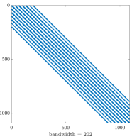
(a) Our approach

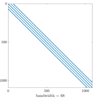
(b) Standard displacement-based Galerkin formulation

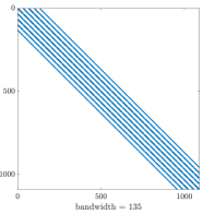
(c) Galerkin mixed formulation, lumped strain projection

Figure 4: Sparsity patterns of the displacement-based system that result from different formulations applied on a square domain, discretized with quadratic B-splines on a mesh of $32\times 32$ elements (after reordering with the minimum degree algorithm).

To put the computing effort for its formation and solution in perspective, we provide the following considerations on the displacement-based system matrix $\mathbf{K}$ in (73):

• The condensed system matrix in our approach remains sparse and banded because its calculation does not involve matrix inversion, unlike for the Galerkin mixed formulation with consistent condensation of the independent strain variables, which leads to a fully populated dense system matrix. Figure 4a illustrates the sparsity pattern for a discretization of a square domain with quadratic B-splines on a mesh of $32\times 32$ Bézier elements (after reordering with the minimum degree algorithm ⁸¹).

• Figures 4b and 4c also show the sparsity pattern for the corresponding system matrices obtained with the standard displacement-based Galerkin formulation and the Galerkin mixed formulation with inconsistent condensation based on row-sum lumping of the projection matrices. We observe that the maximum bandwidth of the condensed matrix in our approach is larger. There are two reasons for that: the first one is that the upper bandwidth of the matrix contributions due to strain condensation, $\mathbf{K}_{12}\mathbf{K}_{21}$ and $\mathbf{K}_{13}\mathbf{K}_{31}$, results from the sum of the corresponding upper bandwidths of the multiplicands ⁸². This also applies to the Galerkin mixed formulation with lumped strain projection, whose condensed system matrix also exhibits a larger bandwidth than the system matrix of the standard Galerkin formulation, see Fig. 4c. The second reason is that the support of an approximate dual function is up to $3p+1$ Bézier elements in each parametric direction, as compared to only $p+1$ for the corresponding B-spline ⁶⁶, which leads to larger upper bandwidths in $\mathbf{K}_{21}$ and $\mathbf{K}_{31}$ as compared to the Galerkin mixed formulation. We deduce from Fig. 4 that the bandwidth increases by about a factor two due to the first reason and by another factor of 1.5 due to the increased support of the approximate dual functions.

• Due to the increased support of the approximate dual functions, the formation of the submatrices $\mathbf{K}_{21}$ and $\mathbf{K}_{31}$ requires more operations than the corresponding submatrices in the Galerkin mixed formulation. For two-dimensional plate and shell elements, we have to expect approximately five to nine times as many basis function related operations to form the two submatrices. In practical scenarios, computationally costly routines to take into account nonlinear material behavior, such as radial return algorithms in plasticity, do not depend on the cost or number of the basis functions of the discrete test space, and hence the net increase in computational cost per quadrature point will be much lower. In addition, only two submatrices of the condensed system matrix in (73) are effected. The submatrices $\mathbf{K}_{11}$, $\mathbf{K}_{12}$ and $\mathbf{K}_{13}$ are equivalent to the Galerkin mixed formulation and therefore incur no additional cost.

• Just as standard B-splines (or NURBS), the modified approximate dual basis functions can be cast into a Bézier or Lagrange extraction format per element ^{83, 84}, whose derivation from relation (6) and the appoximate inverse of the Gramian matrix is straightforward.

• Due to the fact that we discretize the independent strain variables and their variations with different basis functions, the off-diagonal matrices $\mathbf{K}_{12}$ and $\mathbf{K}_{13}$ are not the transpose of their counterparts $\mathbf{K}_{21}$ and $\mathbf{K}_{31}$, and the matrix contributions due to strain condensation are therefore unsymmetric. Solving a system whose coefficient matrix is unsymmetric requires a larger computational effort than solving a symmetric system of the same size, see e.g. ⁸².

Apart from these observations, a precise evaluation of our approach’s computing cost is beyond the scope of this article. While we concentrate here on the numerical properties of the method, the computational performance is influenced by the application context and the quality of the individual computer implementation. In particular, the computational aspects discussed above play a different role depending on whether a direct or iterative solver is used, or if explicit dynamics calculations are performed where the condensed system matrix is never assembled, stored, or inverted.

Remark 6.1.

When we assume the strong satisfaction of the strain-displacement relation for the bending strains, we only discretize discretization the remaining variation of the independent membrane strain field, see Remarks 4.2 and 5.1. The displacement-based matrix equations (73) then become:

$$\left(\mathbf{K}_{11}^{\text{b,mat}}+\tilde{\mathbf{K}}_{11}^{\text{geom}}+\mathbf{K}_{12}\mathbf{K}_{21}\right)\Delta\boldsymbol{\hat{u}}^{h}=\boldsymbol{F}_{ext}-\tilde{\boldsymbol{F}}_{int}-\mathbf{K}_{12}\boldsymbol{F}_{int}^{m}\,.$$ (74)

We note that compared to (73), assembling the right-hand side and the stiffness matrix requires one vector-matrix multiplication fewer and one matrix-matrix multiplication fewer, respectively. Instead, one needs to assemble an additional matrix, $\mathbf{K}_{11}^{\text{b,mat}}$, and the stiffness matrix remains unsymmetric due to the product $\mathbf{K}_{12}\mathbf{K}_{21}$. Although it depends on the implementation, in particular the efficiency of local matrix-matrix products versus the formation of the additional stiffness matrix, the alternative approach of considering only the membrane strains as unknown strain variables does not seem to significantly reduce the computational cost in assembly and solving the matrix equations, compared to our approach of considering both membrane and bending strains as unknown variable fields.

7 Numerical examples

In the following, we demonstrate the favorable numerical properties of higher-order accurate local strain projection based on approximate dual spline functions. We first consider a curved Euler-Bernoulli beam to assess the accuracy in terms of the preservation of higher-order convergence rates and the mitigation of membrane locking as compared to a variety of established methods. We then consider the classical shell obstacle course to showcase the performance of our approach in comparison to other mixed formulations.

Figure 5: A quarter circle steel cantilever represented as a curved Euler-Bernoulli beam, along with boundary and loading conditions.

(a) $p=2$

(b) $p=3$

(c) $p=4$

(d) $p=5$

Figure 6: Curved Euler-Bernoulli beam: relative error in the $L^{2}$-norm of the displacement field, computed with mixed formulations and different methods of strain projection.

(a) $p=2$

(b) $p=3$

(c) $p=4$

(d) $p=5$

Figure 7: Curved Euler-Bernoulli beam: relative error in the $L^{2}$-norm of the displacement field, computed with our approach and different well-established locking-preventing mechanisms.

(a) $p=2$

(b) $p=3$

(c) $p=4$

(d) $p=5$

Figure 8: Curved Euler-Bernoulli beam: spectrum of normalized eigenvalues, computed with mixed formulations and different methods of strain projection and a mesh of 16 Bézier elements.

(a) $p=2$

(b) $p=3$

Figure 9: Curved Euler-Bernoulli beam: lower half of the spectrum of the first 50% of normalized eigenvalues, computed with our approach and different well-established locking-preventing mechanisms and a mesh of 16 elements.

(a) $p=2$

(b) $p=3$

Figure 10: Curved Euler-Bernoulli beam: lower half of the spectrum of the first 50% of normalized eigenvalues, computed with our approach and different well-established locking-preventing mechanisms and a mesh of 32 elements.

7.1 Curved Euler-Bernoulli beam

We consider the boundary value problem of a cantilivered curved Euler-Bernoulli beam illustrated in Fig. 5. Our mixed formulation developed in Sections 4, 5 and 6 for the Kirchhoff-Love shell simplify in a straightforward way to the case of an Euler-Bernoulli beam, and we therefore refrain from presenting details on the formulation. For a detailed exposition of the mixed formulation of the Euler-Bernoulli beam, we refer the interested reader to ⁸.

7.1.1 Convergence study

To conduct a convergence study, we discretize the curved beam with spline basis functions of degree $p=2$ through $p=5$ and conduct uniform $h$-refinement. Our reference is the analytical solution discussed in ⁸⁵ for the quarter circular Euler-Bernoulli cantilever subjected to shear load at the free end. In Fig. 6, we plot the convergence of the relative $L^{2}$ error of the displacement field computed with mixed formulations that evaluate the strain projection part in a different way. To assess our approach, we compare our formulation with independent strain variations discretized by approximate dual functions and row-sum lumping of the strain projection matrix (blue) to the Galerkin mixed formulation with consistent strain projection (black) and the Galerkin mixed formulation with row-sum lumping of the strain projection matrix (red). We note that the consistent Galerkin mixed formulation is prohibitively inefficient, as consistent strain condensation leads to a dense system matrix that is fully populated, but provides the reference accuracy.

We observe that our approach delivers the same accuracy and optimal rates of convergence as the consistent Galerkin mixed formulation for all polynomial degrees. It does not suffer from the significant drop of accuracy that is characteristic for the Galerkin mixed formulation with row-sum lumping, where lumping limits the convergence rate to second-order irrespective of the polynomial degree of the basis functions. We note that the results observed for this example are consistent with the ones observed for the $L^{2}$ projection example in Section 2.3.

To assess the performance of our approach to mitigate membrane locking, we conduct a similar convergence study with different locking-preventing methods for the same curved cantilever (see the introductory section for references on the different methods applied here). In Fig. 7, we plot the convergence of the relative $L^{2}$ error of the displacement field, computed with our approach (blue), a Galerkin mixed formulation with the EAS method (purple), and standard displacement-based Galerkin formulations that mitigate membrane locking via reduced integration (red), the B-bar method (light blue), and the ANS method (yellow). For comparison, we also plot the convergence of the standard Galerkin formulation without any locking-preventing approach (green), fully integrated with $p+1$ Gauss points per Bézier element, which contains the full extent of membrane locking.

Focusing on the results obtained with the standard Galerkin formulation and full integration, we observe the typical pre-asymptotic plateau in the error curves on coarse meshes. In this region, accuracy does not improve with mesh refinement, indicating the severe impact of membrane locking on accuracy and convergence. Increasing the polynomial degree reduces this effect, thereby decreasing the size of the pre-asymptotic plateau. Using the B-bar or the EAS method completely eliminates the effect of locking, leading to optimal convergence rates of $\mathcal{O}(p)$ for $p=2$ and $\mathcal{O}(p+1)$ for $p\geq 3$ ^{86, 87}.

For mixed formulations, the optimal convergence rate obtained for fourth-order problems is $\mathcal{O}(p+1)$ for all $p\geq 1$ ^{86, 87}. Therefore, our approach achieves better accuracy for quadratic discretizations than any of the other methods, and the same accuracy as the B-bar and EAS methods for cubic discretizations and beyond. We also see that our approach eliminates the effect of locking, as it results in error curves that converge directly on coarse meshes with the optimal rate of $\mathcal{O}(p+1)$. We conclude that for fourth-order problems, mixed formulations such as our approach seem to be particularly attractive for quadratic discretizations, for which they achieve better accuracy and a higher rate of convergence than purely displacement-based methods.

7.1.2 Spectral analysis

Based on our prior study in ⁸, we leverage spectral analysis as an alternative tool to assess membrane locking. To this end, we recall the discrete eigenvalue problem of the Euler-Bernoulli beam in matrix form (see e.g. ⁸):

$$\mathbf{K}\,\boldsymbol{U}^{h}_{n}=\lambda^{h}_{n}\,\mathbf{M}\,\boldsymbol{U}^{h}_{n}\,,$$ (75)

where $\boldsymbol{U}^{h}_{n}$ denotes the vector of unknown displacement coefficients corresponding to the $n^{\text{th}}$ discrete eigenmode $U^{h}_{n}$, and $\omega_{n}^{h}$ is the $n^{\text{th}}$ discrete eigenfrequency. We emphasize that in the case of a mixed formulation, the independent strain fields are already condensed out. For the free vibration of the cantilever illustrated in Fig. 5, we compute the discrete eigenvalue $\lambda^{h}$, normalized by the reference value, $\lambda^{h}_{ref}$, which is computed with an “overkill” mesh of 1,024 Bézier elements. We remove the zero eigenvalues associated with rigid body modes, order the remaining non-zero eigenvalues in increasing order and plot the normalized values, $\lambda^{h}/\lambda^{h}_{ref}$, as a function of the normalized mode number, $n/N$.

We first consider, on a mesh of 16 Bézier elements, the same three strain projection variants in the mixed formulation, for which we conducted the convergence study in Fig. 6. In Fig. 8, we compare the spectra obtained with the Galerkin mixed formulation with consistent strain projection (black), which we consider as the reference, the Galerkin mixed formulation with row-sum lumping of the strain projection matrix (red), and our approach based on approximate dual functions for the discretization of the independent strain variations and row-sum lumping of the strain projection matrix (blue). We also provide inset figures that zoom in on the first 50% of the eigenvalues. We observe that compared to the Galerkin mixed formulation with row-sum lumping, our formulation leads to considerably better accuracy over the complete spectrum, in the sense that the spectrum is much closer to the one computed with the consistent Galerkin mixed formulation. We recall that the lowest modes are particularly important for the accuracy of the solution, see e.g. ⁵⁴. In the inset figures, we see that with increasing polynomial degree, the Galerkin mixed formulations with row-sum lumping increasingly deviates from the reference even for the lowest 5% of the modes, while the spectrum curves of the consistent Galerkin mixed formulation and our formulation are practically equivalent within the 20% of the lowest modes. We note that the jump in the spectrum curves around $n/N=0.5$ is due to the chosen ordering and can be eliminated by sorting out different mode types, see ⁸.

We then consider again five of the locking-preventing mechanisms, for which we conducted the convergence study in Fig. 7. In Fig. 10 and 10, we plot the spectral analysis results obtained with a mesh of 16 quadratic and cubic Bézier elements and 32 quadratic and cubic Bézier elements, respectively. The main plots show the first 50% of the eigenvalues, while the inset figures zoom in on the first 20% of the eigenvalues. We compare the spectra obtained with our approach (blue) to the spectra obtained with the standard displacement-based Galerkin formulations that mitigate membrane locking via reduced integration (red), the B-bar method (light blue), and the ANS method (yellow). We note that we exclude the Galerkin mixed formulation with the EAS method, since the results are practically indistinguishable from the ones obtained with the B-bar method, as already observed in the convergence study above. For comparison, we also plot the spectrum of the standard Galerkin formulation without any locking-preventing approach (green), fully integrated with $p+1$ Gauss points per Bézier element, which includes the full extent of membrane locking. We note that jumps in the spectrum curves occur due to the chosen ordering and can be eliminated by sorting out different mode types.

The results shown here for the the standard displacement-based Galerkin formulation with different locking-preventing mechanisms confirm what we reported in our earlier study ⁸. We observe that the B-bar method (and the EAS method) are particularly successful in completely removing any effect of membrane locking. In addition, we observe that our approach delivers excellent spectral accuracy for the lowest modes. It exhibits a distinct decay of spectral accuracy for the medium and high modes, which is typical for mixed formulations with condensed strain variables ⁸. The spectrum results in Fig. 10a and 10a also confirm the above observation that our approach achieves better accuracy for quadratic discretizations than any of the other locking-preventing methods. For the case of quadratic basis functions, we observe that in the critical lower modes, the spectrum curve of our mixed formulation is much closer to the optimum value of one than the spectrum curves of all the other methods, including the B-bar method.

(a) $p=2$

(b) $p=3$

(c) $p=4$

(d) $p=5$

Figure 11: Curved Euler-Bernoulli beam: relative error in the $L^{2}$-norm of the displacement field, computed with our approach and two different projection variants. $\mathbb{S}^{p,r}_{n}$ denotes a space spanned by $n$ B-splines basis functions of polynomial degree $p$ with continuity $C^{r}$.

(a) $\varepsilon^{h}$

(b) $\kappa^{h}$

Figure 12: Curved Euler-Bernoulli beam: membrane strain and the change of curvature, computed with our approach and two different projection variants on a mesh of 8 cubic elements. $\mathbb{S}^{p,r}_{n}$ denotes a space spanned by $n$ B-splines basis functions of polynomial degree $p$ with continuity $C^{r}$.

7.1.3 Assessment of different strain projection variants

We use the same benchmark of the curved cantilever beam to carry out a similar convergence study to assess the performance of our approach with the two different strain projection variants: (a) strain projection of the membrane and bending strains, where both strains are discretized with basis functions of one polynomial order lower than the displacements (plotted in blue), and (b) strain projection of only membrane strains, discretized with basis functions of one order lower than the displacements (plotted in red), along the Remarks 4.2, 5.1, and 6.1.

In Fig. 11, we plot the convergence of the relative $L^{2}$ error of the displacement field, computed with our approach and the above strain projection variants. Focusing on the results obtained with quadratic basis functions, we observe that strain projection of only the membrane strains leads to a reduction of the optimal convergence rate to  $\mathcal{O}(p)$ for $p=2$ ^{86, 87}, since we deal with a fourth-order problem due to the strong enforcement of the bending kinematics, see also Remark 4.2. In case of the projection of both the membrane and bending strains, we deal with a second-order problem, and thus are able to achieve the optimal rate of $\mathcal{O}(p+1)$ for all $p\geq 1$^{86, 87}. This constitutes a distinct advantage of the latter for quadratic spline discretizations. Focusing on the results obtained with cubic, quartic, and quintic splines, we observe that the two projection variants achieve a comparable accuracy, both in terms of convergence rate and preasymptotic error level, irrespective of the number of the projected strain fields and the degree of basis functions employed for the bending strains $\kappa$.

In Fig. 12, we plot the discrete membrane and bending strains, obtained with the two projection variants, as a function of the angular coordinate $\theta$. For comparison, we also plot the analytical solution (see ⁸⁵ for its derivation). We include inset figures which focus on the results close to the boundary with clamped support. We observe that the projection of only the membrane strains results in bending strains that exhibit distinct oscillations. In the case of projecting both membrane and bending strains, these oscillations are absent. These observations confirm that our choice of projecting both membrane and bending strains has some advantages over the alternative of projecting only the membrane strains, and we there adopt this variants in the remainder of this work.

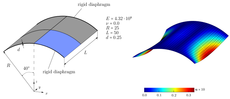
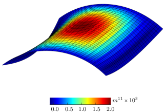
Figure 13: Scordelis-Lo roof constrained by rigid diaphragms and subjected to its self-weight of $90.0$ per unit area: problem sketch along with plots of the deformed configuration and the stress resultant $m^{11}$, computed with our approach and quadratic splines. The deformations are illustrated with displacements scaled by a factor of $10$.

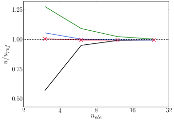
(a) $p=2$

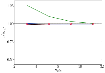
(b) $p=3$

Figure 14: Scordelis-Lo roof: convergence of the normalized vertical displacement at the midpoint of the free edge, computed with different formulations.

(a) $p=2$

(b) $p=3$

(c) $p=4$

(d) $p=5$

Figure 15: Scordelis-Lo roof: convergence of the relative error in the $H^{2}$ semi-norm in the stress resultant $m^{12}$, computed with different formulations.

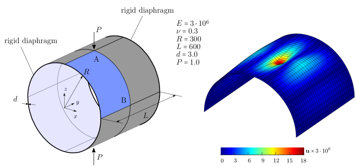
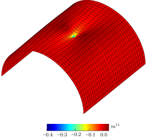
Figure 16: Pinched cylinder constrained by rigid diaphragms: problem sketch along with plots of the deformed configuration and the stress resultant $m^{11}$, computed with our approach and quadratic splines. The deformations are illustrated with displacements scaled by a factor of $3\cdot 10^{6}$.

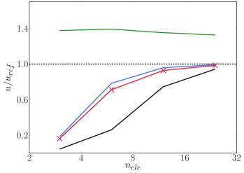
(a) $p=2$

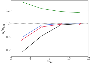
(b) $p=3$

Figure 17: Pinched cylinder: convergence of the normalized displacement under the load, computed with different formulations.

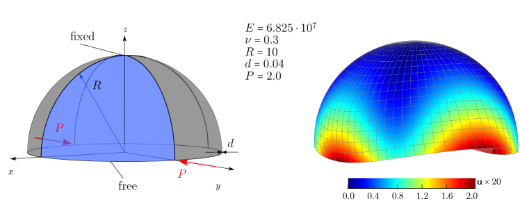
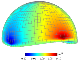
Figure 18: Hemispherical shell fixed at the top: problem sketch along with plots of the deformed configuration and the stress resultant $m^{11}$, computed with our approach and quadratic splines. The deformations are illustrated with displacements scaled by a factor of $20$.

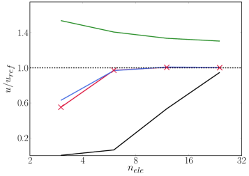
(a) $p=2$

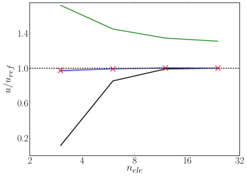
(b) $p=3$

Figure 19: Hemispherical shell: convergence of the normalized radial displacement under the load, computed with different formulations.

(a) $p=2$

(b) $p=3$

(c) $p=4$

(d) $p=5$

Figure 20: Hemispherical shell: convergence of the relative error in the $H^{2}$ semi-norm in the stress resultant $m^{12}$, computed with different formulations.

7.2 The classical shell obstacle course

We now move to the Kirchhoff-Love shell problem and demonstrate the performance of our mixed formulation for the three elastostatic examples of the classical shell obstacle course ¹⁰. We compare our formulation based on approximate dual functions for the discretization of the independent strain variations and row-sum lumping of the resulting strain projection matrix to the standard displacement-based Galerkin formulation ⁷³, the (computationally inefficient) Galerkin mixed formulation with consistent strain projection, which serves as the reference in terms of accuracy, and the Galerkin mixed formulation with row-sum lumping of the strain projection matrix, which is equivalent in terms of strain condensation.

7.2.1 Scordelis-Lo roof

The first example consists of the Scordelis-Lo roof subjected to its self-weight of 90.0 per unit area, illustrated in Fig. 14. For discretization, we exploit the symmetry and model only a quarter of the structure marked in blue. Figure 14 also illustrates the deformed configuration and the stress resultant $m^{11}$, computed with our formulation and quadratic splines on a $16\times 16$ mesh.

In Fig. 14, we plot the convergence of the normalized displacement at the midpoint of the free edge, for which a reference solution exists, see e.g. ^{10, 73}. We observe that the standard Galerkin formulation (black) leads to inaccurate results on coarse meshes, likely a result of membrane locking. This effect is reduced when we increase the polynomial degree of the basis functions from quadratics to cubics. We also see that the Galerkin mixed formulation with row-sum lumping of the strain projection matrix (green) leads to significant errors that do not vanish with increasing polynomial degrees. Consistent with the observations for the beam example, we see that our strain projection approach (blue) leads to results that are very close to the ones of the consistent Galerkin mixed formulation (red).

In the next step, we carry out uniform $h$-refinement using the sequence of 3, 6, 12, and 24 Bézier elements per edge and smooth splines of degree $p=2$ through $p=5$. In Fig. 15, we plot the convergence of the relative error in the $H^{2}$ semi-norm in the stress resultant $m^{12}$. The error is computed with respect to an overkill solution, computed with the Galerkin mixed formulation on a mesh of $128\times 128$ Bézier elements and smooth B-splines of degree $p=7$. We observe that the standard Galerkin formulation (black) shows a slightly higher error level on coarse meshes, but converges to the same error level as the consistent Galerkin mixed formulation (red). Increasing the polynomial degree of the basis functions reduces this error difference also for coarser meshes. When we compare the results obtained with the consistent mixed Galerkin formulation (red) and the mixed Galerkin formulation with lumped strain projection matrix (green), we see that the latter leads to significantly larger errors and the same linear convergence irrespective of the polynomial degree. This is consistent with the observations above and illustrates the dominating impact of row-sum lumping on the accuracy and convergence of the corresponding discretization scheme. When we focus on our formulation (blue) and the consistent Galerkin mixed formulation (red), we observe that the former shows a slightly higher error level than the latter. Nevertheless, the error associated with our approach remains very close (within the same order of magnitude) and converges with the optimal rate of convergence, $\mathcal{O}(p-1)$ ^{86, 87}, when the mesh is refined.

7.2.2 Pinched cylinder

The second example consists of a pinched cylinder subjected to two opposite unit loads in the middle, illustrated in Fig. 16. We again exploit the symmetry and model only one-eighth of the structure marked in blue. Figure 16 also illustrate the deformed configuration and the stress resultant $m^{11}$, computed with our formulation and quadratic splines on a $16\times 16$ mesh.

In Fig. 17, we plot the convergence of the normalized displacement at point A under the pinching load, for which reference solutions exist, see e.g. ^{10, 73}. We observe the same behavior as before. The standard Galerkin formulation (black) leads to largely inaccurate results that are too stiff, likely amplified by membrane locking, in particular for coarse meshes. The results of our formulation (blue) are considerably better and very close to the results of the consistent Galerkin mixed formulation (red). Row-sum lumping of the strain projection matrix in the Galerkin mixed formulation (green) leads to a persistent error and prevents convergence. We report that the error in the $H^{2}$ semi-norm is dominated by the stress singularity under the loading point, so that its convergence is linear for all methods. Therefore, we refrain from including the corresponding plots here.

7.2.3 Hemispherical shell

The third example consists of a hemispherical shell subjected to two opposite loads in the $xy$-plane, illustrated in Fig. 19. We also exploit the symmetry and model only a quarter of the structure marked in blue. Figure 19 also illustrates the deformed configuration and the stress resultant $m^{11}$, computed with our formulation and quadratic splines on a $16\times 16$ mesh.

In Fig. 19, we plot the convergence of the normalized radial displacement at the pinched point under the load, for which reference solutions exist, see e.g. ^{10, 73}. Similarly to the Scordelis-Lo roof and the pinched cylinder, we observe that the standard Galerkin formulation (black) exhibits results on coarse meshes that are largely too stiff, likely due to membrane locking. This effect is reduced when we increase the polynomial degree of the basis functions from quadratics to cubics. We also see that the Galerkin mixed formulation with row-sum lumping of the strain projection matrix (green) leads to significant errors that do not vanish with increasing polynomial degrees. Consistent with the observations for the beam example, we see that our strain projection approach (blue) effectively eliminates the locking effect on coarse meshes and leads to results that are very close to and for the most part practically indistinguishable from the ones of the consistent Galerkin mixed formulation (red).

In the next step, we carry out uniform $h$-refinement at fixed polynomial degrees $p=2$ through $p=5$. In Fig. 20, we plot the convergence of the relative error in the $H^{2}$ semi-norm in the stress resultant $m^{12}$ with respect to an overkill solution, computed again with the Galerkin mixed formulation on a mesh of $128\times 128$ Bézier elements and splines of degree $p=7$.

We observe that the standard Galerkin formulation (black) leads to significant errors on coarse meshes. Particularly in the case of quadratic spline functions, we see a clear pre-asymptotic plateau similar to the one observed earlier for the curved Euler-Bernoulli beam, a typical sign of membrane locking. Increasing the polynomial degree of the basis functions removes this plateau, also for coarser meshes. We observe that our formulation (blue) effectively removes the locking effect, also on coarse meshes with moderate polynomial degree, and its results are practically indistinguishable from the results of the consistent Galerkin mixed formulation (red).

8 Summary and conclusions

We presented a novel discretization strategy for the mixed variational formulation of the Kirchhoff-Love shell problem, derived from the modified Hellinger-Reissner variational principle. For mitigating membrane locking, we discretized the independent strain fields with spline basis functions that are one degree lower than those used for the displacements. The key novelty of our approach is the utilization of approximate dual spline functions to discretize the variations of the independent strain fields. We demonstrated that the resulting nearly diagonal submatrices of the strain projection equations can then be diagonalized by row-sum lumping without loss of higher-order accuracy. Thus, the diagonalized projection matrices enable the direct condensation of the independent strain variables, resulting in a purely displacement-based system matrix, while the full accuracy of the mixed formulation can be retained for any polynomial degree of the approximation.

We demonstrated the higher-oder accuracy of our approach and the mitigation of membrane locking with numerical benchmarks, including a curved Euler-Bernoulli beam and the examples of the shell obstacle course. We also showed for these examples that our approach achieves practically the same accuracy as the Galerkin mixed formulation with consistent strain condensation (which is prohibitively expensive from a computing viewpoint), while it eliminates membrane locking as effectively as the best out of a number of well-established locking-preventing methods, applied in the standard Galerkin formulation. Our results confirmed that for quadratic discretizations of Kirchhoff-Love shell problems, our approach based on the projection of both the membrane and bending strains is particularly attractive, as mixed formulations achieve better accuracy than any of the other methods in the context of the standard displacement-based Galerkin formulation. For us, this result seems particularly noteworthy, as the industrial focus at this point in time is reported to be on quadratic spline discretizations.

From a computational perspective, our formulation considerably reduces the computing effort associated with storing and solving a significantly larger system that emanates from a mixed variational formulation. We discussed that there is still a larger computational effort involved in comparison with the standard displacement-based Galerkin formulation. On the one hand, one needs to compute more operations at the quadrature point level when forming the condensed displacement-based system matrix. One the other hand, the condensed system matrix exhibits an increased bandwidth and is unsymmetric. These computational aspects play a different role depending on whether a direct or iterative solver is used, or if explicit dynamics calculations are performed where the condensed system matrix is never assembled, stored, or factorized. Ultimately, in each setting, the crucial point is that a competitive method achieves a given level of accuracy more quickly than its competitors, using comparable or fewer computing resources. In the realm of higher-order accurate isogeometric shell analysis, we believe that our approach presented in this paper has the potential to perform competitively. This will be the subject of more detailed future studies. A particularly interesting aspect is the synergistic combination of the properties of approximate dual spline functions for strain condensation and mass lumping in explicit dynamics ^{66, 67} as well as outlier removal methods for the control of the maximum time step ^{88, 89}.

*Acknowledgments

The authors gratefully acknowledge financial support from the German Research Foundation (Deutsche Forschungsgemeinschaft) through the DFG Emmy Noether Grant SCH 1249/2-1 and the standard DFG grant SCH 1249/5-1.

Appendix A Linearization of the membrane and bending strains

We obtain the strain-displacement matrix $\mathbf{B}^{m}$ corresponding to the membrane strains via substituting (41) into (19):

$$\delta\boldsymbol{\varepsilon}^{h}=\begin{bmatrix}\delta\varepsilon_{11}^{h}\\ \delta\varepsilon_{22}^{h}\\ 2\delta\varepsilon_{12}^{h}\end{bmatrix}=\sum_{i=1}^{n}\,\underbrace{\begin{bmatrix}\boldsymbol{a}_{1}^{T}\,B_{i,1}\\ \boldsymbol{a}_{2}^{T}\,B_{i,2}\\ \boldsymbol{a}_{1}^{T}\,B_{i,2}+\boldsymbol{a}_{2}^{T}\,B_{i,1}\end{bmatrix}}_{\mathbf{B}^{m}_{i}}\,\delta\boldsymbol{\hat{u}}^{h}_{i}=\sum_{i=1}^{n}\,\mathbf{B}^{m}_{i}\,\delta\boldsymbol{\hat{u}}^{h}_{i}\,,$$ (76)

where $\delta\boldsymbol{\hat{u}}^{h}$ is the variation of the vector of unknown coefficients $\boldsymbol{\hat{u}}_{i}^{h}$ in (41). Here, the covariant base vectors $\boldsymbol{a}_{1}$ and $\boldsymbol{a}_{2}$ are computed using the discrete position vector of the midsurface, $\boldsymbol{\bar{x}}^{h}$, in the current configuration:

$$\boldsymbol{a}_{1}=\boldsymbol{\bar{x}}^{h}_{,1}\,,\qquad\boldsymbol{a}_{2}=\boldsymbol{\bar{x}}^{h}_{,2}\,.$$ (77)

To derive the strain-displacement matrix $\mathbf{B}^{b}$, we first compute the variation of the normalized normal vector $\boldsymbol{a}_{3}$ (14) as follows:

$$\delta\boldsymbol{a}_{3}=\frac{1}{\left\|\boldsymbol{n}_{3}\right\|}\,\underbrace{\left(\mathbf{I}-\boldsymbol{a}_{3}\otimes\boldsymbol{a}_{3}\right)}_{\mathbf{P}}\,\delta\boldsymbol{n}_{3}=\frac{1}{\left\|\boldsymbol{n}_{3}\right\|}\,\mathbf{P}\,\delta\boldsymbol{n}_{3}\,,\quad\text{with}\quad\boldsymbol{n}_{3}=\boldsymbol{a}_{1}\times\boldsymbol{a}_{2}\,,$$ (78)

and $\left\|\boldsymbol{n}_{3}\right\|$ denotes the norm of the normal vector $\boldsymbol{n}_{3}$. Substituting this and (41) into (20) leads to:

$$\delta\boldsymbol{\kappa}^{h}=\begin{bmatrix}\delta\kappa_{11}^{h}\\ \delta\kappa_{22}^{h}\\ 2\delta\kappa_{12}^{h}\end{bmatrix}=\,\sum_{i=1}^{n}\,\underbrace{\begin{bmatrix}-\boldsymbol{a}_{3}^{T}B_{i,11}-\frac{1}{\left\|\boldsymbol{n}_{3}\right\|}\,\left[\boldsymbol{a}_{2}\times\left(\mathbf{P}\,\boldsymbol{a}_{1,1}\right)\right]^{T}B_{i,1}+\frac{1}{\left\|\boldsymbol{n}_{3}\right\|}\,\left[\boldsymbol{a}_{1}\times\left(\mathbf{P}\,\boldsymbol{a}_{1,1}\right)\right]^{T}B_{i,2}\\ -\boldsymbol{a}_{3}^{T}B_{i,22}-\frac{1}{\left\|\boldsymbol{n}_{3}\right\|}\,\left[\boldsymbol{a}_{2}\times\left(\mathbf{P}\,\boldsymbol{a}_{2,2}\right)\right]^{T}B_{i,1}+\frac{1}{\left\|\boldsymbol{n}_{3}\right\|}\,\left[\boldsymbol{a}_{1}\times\left(\mathbf{P}\,\boldsymbol{a}_{2,2}\right)\right]^{T}B_{i,2}\\ -2\boldsymbol{a}_{3}^{T}B_{i,12}-\frac{2}{\left\|\boldsymbol{n}_{3}\right\|}\,\left[\boldsymbol{a}_{2}\times\left(\mathbf{P}\,\boldsymbol{a}_{1,2}\right)\right]^{T}B_{i,1}+\frac{2}{\left\|\boldsymbol{n}_{3}\right\|}\,\left[\boldsymbol{a}_{1}\times\left(\mathbf{P}\,\boldsymbol{a}_{1,2}\right)\right]^{T}B_{i,2}\end{bmatrix}}_{\mathbf{B}^{b}_{i}}\,\delta\boldsymbol{\hat{u}}^{h}_{i}=\sum_{i=1}^{n}\,\mathbf{B}^{b}_{i}\,\delta\boldsymbol{\hat{u}}^{h}_{i}$$ (79)

To derive the geometric stiffness matrix (48), we start with the second variation of the membrane strains. Substituting (41) into (21), we obtain:

$$\Delta\delta\varepsilon_{\alpha\beta}^{h}=\sum_{i=1}^{n}\,\sum_{j=1}^{n}\,\frac{1}{2}\,\left(\delta\boldsymbol{\hat{u}}^{h}_{i}\right)^{T}\left(B_{i,\alpha}\,B_{j,\beta}+B_{i,\beta}\,B_{j,\alpha}\right)\,\mathbf{I}\,\Delta\boldsymbol{\hat{u}}^{h}_{j}\,.$$ (80)

The membrane part of the geometric stiffness matrix, $\mathbf{K}_{11}^{\text{m,geom}}$, associated to the $i$-th and $j$-th control point is:

$$\mathbf{K}_{11,ij}^{\text{m,geom}}=\sum_{\alpha=1}^{2}\,\sum_{\beta=1}^{2}\,\frac{1}{2}\,\left(B_{i,\alpha}\,B_{j,\beta}+B_{i,\beta}\,B_{j,\alpha}\right)\,\bar{n}_{\alpha\beta}^{h}\,\mathbf{I}\,,$$ (81)

where $\bar{n}_{\alpha\beta}^{h}$ is the stress resultant for the discrete normal force components corresponding to the independent membrane strain variables $\boldsymbol{e}$ in (34), i.e.:

$$\begin{bmatrix}\bar{n}^{h}_{11}\\ \bar{n}^{h}_{22}\\ \bar{n}^{h}_{12}\end{bmatrix}=d\,\mathbf{C}\,\boldsymbol{e}^{h}\,.$$ (82)

The variation and linearization of the normal vector $\boldsymbol{n}_{3}$ are:

$$\delta\boldsymbol{n}_{3} =\delta\boldsymbol{a}_{1}\times\boldsymbol{a}_{2}+\boldsymbol{a}_{1}\times\delta\boldsymbol{a}_{2}=\boldsymbol{a}_{1}\times\delta\boldsymbol{a}_{2}-\boldsymbol{a}_{2}\times\delta\boldsymbol{a}_{1}$$

$$=\sum_{i=1}^{n}\,\underbrace{\left(\left[\boldsymbol{a}_{1}\right]_{\times}\,B_{i,2}-\left[\boldsymbol{a}_{2}\right]_{\times}\,B_{i,1}\right)}_{\mathbf{A}_{i}}\,\delta\boldsymbol{\hat{u}}^{h}_{i}=\sum_{i=1}^{n}\,\mathbf{A}_{i}\,\delta\boldsymbol{\hat{u}}^{h}_{i}\,,$$ (83)

$$\Delta\boldsymbol{n}_{3} =\sum_{i=1}^{n}\,\mathbf{A}_{i}\,\Delta\boldsymbol{\hat{u}}^{h}_{i}\,,$$ (84)

respectively, where $\left[\boldsymbol{a}_{\alpha}\right]_{\times}$ is the skew-symmetric matrix of vector $\boldsymbol{a}_{\alpha}$. The linearization of the variation of the normalized normal vector $\boldsymbol{a}_{3}$ (78) is:

$$\Delta\delta\boldsymbol{a}_{3}=-\frac{1}{\left\|\boldsymbol{n}_{3}\right\|^{2}}\left(\boldsymbol{a}_{3}\cdot\Delta\boldsymbol{n}_{3}\right)\,\mathbf{P}\,\delta\boldsymbol{n}_{3}-\frac{1}{\left\|\boldsymbol{n}_{3}\right\|}\left(\Delta\boldsymbol{a}_{3}\otimes\boldsymbol{a}_{3}+\boldsymbol{a}_{3}\otimes\Delta\boldsymbol{a}_{3}\right)\,\delta\boldsymbol{n}_{3}\,.$$ (85)

Inserting this and (41) into (22) leads to:

$$\Delta\delta\kappa_{\alpha\beta}^{h}=\sum_{i=1}^{n}\,\sum_{j=1}^{n}\,\left(\delta\boldsymbol{\hat{u}}^{h}_{i}\right)^{T}\left\{-\frac{1}{\left\|\boldsymbol{n}_{3}\right\|}B_{i,\alpha\beta}\mathbf{P}\,\mathbf{A}_{j}+\frac{1}{\left\|\boldsymbol{n}_{3}\right\|}\mathbf{A}_{i}\,\mathbf{P}\,B_{j,\alpha\beta}-\frac{1}{\left\|\boldsymbol{n}_{3}\right\|^{2}}\mathbf{A}_{i}\left[2\boldsymbol{a}_{3}\odot\boldsymbol{a}_{\alpha,\beta}+\left(\boldsymbol{a}_{3}\cdot\boldsymbol{a}_{\alpha,\beta}\right)\left(\mathbf{I}-3\boldsymbol{a}_{3}\otimes\boldsymbol{a}_{3}\right)\right]\,\mathbf{A}_{j}\right\}\,\Delta\boldsymbol{\hat{u}}^{h}_{j}\,,$$ (86)

where $\odot$ denotes the symmetric product of two vectors, i.e.:

$$\boldsymbol{a}_{3}\odot\boldsymbol{a}_{\alpha,\beta}=\frac{1}{2}\left(\boldsymbol{a}_{3}\otimes\boldsymbol{a}_{\alpha,\beta}+\boldsymbol{a}_{\alpha,\beta}\otimes\boldsymbol{a}_{3}\right)\,.$$ (87)

The bending part of the geometric stiffness matrix, $\mathbf{K}_{11}^{\text{b,geom}}$, associated to the $i$-th and $j$-th control point is:

$$\mathbf{K}_{11,ij}^{\text{b,geom}}=\sum_{\alpha=1}^{2}\,\sum_{\beta=1}^{2}\,\bar{m}_{\alpha\beta}^{h}\,\left\{-\frac{1}{\left\|\boldsymbol{n}_{3}\right\|}B_{i,\alpha\beta}\mathbf{P}\,\mathbf{A}_{j}+\frac{1}{\left\|\boldsymbol{n}_{3}\right\|}\mathbf{A}_{i}\,\mathbf{P}\,B_{j,\alpha\beta}-\frac{1}{\left\|\boldsymbol{n}_{3}\right\|^{2}}\mathbf{A}_{i}\left[2\boldsymbol{a}_{3}\odot\boldsymbol{a}_{\alpha,\beta}+\left(\boldsymbol{a}_{3}\cdot\boldsymbol{a}_{\alpha,\beta}\right)\left(\mathbf{I}-3\boldsymbol{a}_{3}\otimes\boldsymbol{a}_{3}\right)\right]\,\mathbf{A}_{j}\right\}\,,$$ (88)

where $\bar{m}_{\alpha\beta}^{h}$ is the stress resultant for the discrete bending moment components components corresponding to the independent variables $\boldsymbol{k}$ in (34), i.e.:

$$\begin{bmatrix}\bar{m}^{h}_{11}\\ \bar{m}^{h}_{22}\\ \bar{m}^{h}_{12}\end{bmatrix}=\frac{d^{3}}{12}\,\mathbf{C}\,\boldsymbol{k}^{h}\,.$$ (89)

Analogously, $\tilde{\mathbf{K}}_{11,ij}^{\text{b,geom}}$, associated to the $i$-th and $j$-th control point is:

$$\tilde{\mathbf{K}}_{11,ij}^{\text{b,geom}}=\sum_{\alpha=1}^{2}\,\sum_{\beta=1}^{2}\,m_{\alpha\beta}^{h}\,\left\{-\frac{1}{\left\|\boldsymbol{n}_{3}\right\|}B_{i,\alpha\beta}\mathbf{P}\,\mathbf{A}_{j}+\frac{1}{\left\|\boldsymbol{n}_{3}\right\|}\mathbf{A}_{i}\,\mathbf{P}\,B_{j,\alpha\beta}-\frac{1}{\left\|\boldsymbol{n}_{3}\right\|^{2}}\mathbf{A}_{i}\left[2\boldsymbol{a}_{3}\odot\boldsymbol{a}_{\alpha,\beta}+\left(\boldsymbol{a}_{3}\cdot\boldsymbol{a}_{\alpha,\beta}\right)\left(\mathbf{I}-3\boldsymbol{a}_{3}\otimes\boldsymbol{a}_{3}\right)\right]\,\mathbf{A}_{j}\right\}\,,$$ (90)

where $m_{\alpha\beta}^{h}$ is the stress resultant for the discrete bending moment components components corresponding to the displacement-based variables $\boldsymbol{\kappa}$ in (17), i.e.:

$$\begin{bmatrix}m^{h}_{11}\\ m^{h}_{22}\\ m^{h}_{12}\end{bmatrix}=\frac{d^{3}}{12}\,\mathbf{C}\,\boldsymbol{\kappa}^{h}\,.$$ (91)

References

- 1 Hughes TJR, Cottrell JA, Bazilevs Y. Isogeometric analysis: CAD, finite elements, NURBS, exact geometry and mesh refinement. Computer methods in applied mechanics and engineering 2005; 194(39-41): 4135–4195.
- 2 Haberleitner M, Jüttler B, Scott M, Thomas D. Isogeometric Analysis: Representation of Geometry. In: Stein E, Borst dR, Hughes TJR. , eds. Encyclopedia of Computational Mechanics 2nd EditionWiley. 2017.
- 3 Stolarski H, Belytschko T. Membrane locking and reduced integration for curved elements. Journal of Applied Mechanics, Transactions ASME 1982; 49(1): 172–176.
- 4 Stolarski H, Belytschko T. Shear and membrane locking in curved C0 elements. Computer Methods in Applied Mechanics and Engineering 1983; 41(3): 279–296.
- 5 Bischoff M, Wall WA, Bletzinger KU, Ramm E. Models and Finite Elements for Thin-walled Structures. In: Stein E, Borst dR, Hughes TJR. , eds. Encyclopedia of Computational Mechanics. 2. John Wiley & Sons. 2004 (pp. 59–137).
- 6 Hughes TJR. The Finite Element Method: Linear Static and Dynamic Finite Element Analysis. Dover Publications . 2003.
- 7 Echter R, Bischoff M. Numerical efficiency, locking and unlocking of NURBS finite elements. Computer Methods in Applied Mechanics and Engineering 2010; 199: 374–382.
- 8 Nguyen TH, Hiemstra RR, Schillinger D. Leveraging spectral analysis to elucidate membrane locking and unlocking in isogeometric finite element formulations of the curved Euler–Bernoulli beam. Computer Methods in Applied Mechanics and Engineering 2022; 388: 114240.
- 9 Hiemstra RR, Fuentes F, Schillinger D. Fourier analysis of membrane locking and unlocking. Computer Methods in Applied Mechanics and Engineering 2023: 116353.
- 10 Belytschko T, Stolarski H, Liu WK, Carpenter N, Ong JS. Stress projection for membrane and shear locking in shell finite elements. Computer Methods in Applied Mechanics and Engineering 1985; 51(1-3): 221–258.
- 11 Hughes TJ. Equivalence of finite elements for nearly incompressible elasticity. Journal of Applied Mechanics 1977; 44: 181–183.
- 12 Hughes TJ. Generalization of selective integration procedures to anisotropic and nonlinear media. International Journal for Numerical Methods in Engineering 1980; 15(9): 1413–1418.
- 13 Recio DP, Jorge RMN, Dinis LMS. Locking and hourglass phenomena in an element-free Galerkin context: the B-bar method with stabilization and an enhanced strain method. International Journal for Numerical Methods in Engineering 2006; 68(13): 1329–1357.
- 14 Simo JC, Hughes TJ. On the variational foundations of assumed strain methods. Journal of Applied Mechanics, Transactions ASME 1986; 53(1): 51–54.
- 15 Bucalem ML, Bathe KJ. Higher-order MITC general shell elements. International Journal for Numerical Methods in Engineering 1993; 36(21): 3729–3754.
- 16 Bathe KJ, Dvorkin EN. Short Communication a Four-Node Plate Bending Element Based on Mindlin / Reissner Plate Theory and. International Journal for Numerical Methods in Engineering 1985; 21(March 1984): 367–383.
- 17 Andelfinger U, Ramm E. EAS-elements for two-dimensional, three-dimensional, plate and shell structures and their equivalence to HR-elements. International Journal for Numerical Methods in Engineering 1993; 36(8): 1311–1337.
- 18 Bischoff M, Ramm E, Braess D. A class of equivalent enhanced assumed strain and hybrid stress finite elements. Computational Mechanics 1999; 22(6): 443–449.
- 19 Alves de Sousa RJ, Cardoso RP, Fontes Valente RA, Yoon JW, Grácio JJ, Natal Jorge RM. A new one-point quadrature enhanced assumed strain (EAS) solid-shell element with multiple integration points along thickness: Part I - Geometrically linear applications. International Journal for Numerical Methods in Engineering 2005; 62(7): 952–977.
- 20 Zienkiewicz OC, Taylor RL, Too JM. Reduced integration technique in general analysis of plates and shells. International Journal for Numerical Methods in Engineering 1971; 3(2): 275-290.
- 21 Malkus DS, Hughes TJ. Mixed finite element methods - Reduced and selective integration techniques: A unification of concepts. Computer Methods in Applied Mechanics and Engineering 1978; 15(1): 63–81.
- 22 Noor AK, Peters JM. Mixed Models and Reduced/Selective Integration Displacement Models for Nonlinear Shell Analysis.. American Society of Mechanical Engineers, Applied Mechanics Division, AMD 1981; 48(April 1980): 119–146.
- 23 Schwarze M, Reese S. A reduced integration solid-shell finite element based on the EAS and the ANS concept-Geometrically linear problems. International Journal for Numerical Methods in Engineering 2009; 80(10): 1322–1355.
- 24 Flanagan DP, Belytschko T. A uniform strain hexahedron and quadrilateral with orthogonal hourglass control. International Journal for Numerical Methods in Engineering 1981; 17(5): 679–706.
- 25 Belytschko T, Ong JSJ. Hourglass control in linear and nonlinear problems. Computer Methods in Applied Mechanics and Engineering 1984; 43: 251–276.
- 26 Reese S. A large deformation solid-shell concept based on reduced integration with hourglass stabilization. International Journal for Numerical Methods in Engineering 2007; 69(8): 1671–1716.
- 27 Kim JG, Kim YY. A new higher-order hybrid-mixed curved beam element. International Journal for Numerical Methods in Engineering 1998; 43(5): 925–940.
- 28 Klinkel S, Gruttmann F, Wagner W. A mixed shell formulation accounting for thickness strains and finite strain 3D material models. International Journal for Numerical Methods in Engineering 2008; 74(6): 945–970.
- 29 Stolarski H, Belytschko T. On the equivalence of mode decomposition and mixed finite elements based on the Hellinger-Reissner principle. Part I: Theory. Computer Methods in Applied Mechanics and Engineering 1986; 58(3): 249–263.
- 30 Lee Y, Yoon K, Lee PS. Improving the MITC3 shell finite element by using the Hellinger–Reissner principle. Computers & Structures 2012; 110-111: 93–106.
- 31 Ashwell DG, Gallagher R. Finite elements for thin shells and curved members. London: John Wiley & Sons, Ltd . 1976.
- 32 Rank E, Krause R, Preusch K. On the accuracy of p-version elements for the Reissner-Mindlin plate problem. International Journal for Numerical Methods in Engineering 1998; 43(1): 51–67.
- 33 Greco L, Cuomo M, Contrafatto L, Gazzo S. An efficient blended mixed B-spline formulation for removing membrane locking in plane curved Kirchhoff rods. Computer Methods in Applied Mechanics and Engineering 2017; 324: 476–511.
- 34 Bouclier R, Elguedj T, Combescure A. Locking free isogeometric formulations of curved thick beams. Computer Methods in Applied Mechanics and Engineering 2012; 245-246: 144–162.
- 35 Beirão da Veiga L, Lovadina C, Reali A. Avoiding shear locking for the Timoshenko beam problem via isogeometric collocation methods. Computer Methods in Applied Mechanics and Engineering 2012; 241-244: 38–51.
- 36 Bieber S, Oesterle B, Ramm E, Bischoff M. A variational method to avoid locking-independent of the discretization scheme. International Journal for Numerical Methods in Engineering 2018; 114(8): 801–827.
- 37 Zhang G, Alberdi R, Khandelwal K. On the locking free isogeometric formulations for 3-D curved Timoshenko beams. Finite Elements in Analysis and Design 2018; 143: 46–65.
- 38 Elguedj T, Bazilevs Y, Calo VM, Hughes TJ. B-bar and F-bar projection methods for nearly incompressible linear and non-linear elasticity and plasticity using higher-order NURBS elements. Computer Methods in Applied Mechanics and Engineering 2008; 197(33-40): 2732–2762.
- 39 Adam C, Hughes TJ, Bouabdallah S, Zarroug M, Maitournam H. Selective and reduced numerical integrations for NURBS-based isogeometric analysis. Computer Methods in Applied Mechanics and Engineering 2015; 284(August): 732–761.
- 40 Adam C, Bouabdallah S, Zarroug M, Maitournam H. Improved numerical integration for locking treatment in isogeometric structural elements. Part II: Plates and shells. Computer Methods in Applied Mechanics and Engineering 2015; 284: 106–137.
- 41 Benson DJ, Bazilevs Y, Hsu MC, Hughes TJR. Isogeometric shell analysis: The Reissner-Mindlin shell. Computer Methods in Applied Mechanics and Engineering 2010; 199: 276–289.
- 42 Bouclier R, Elguedj T, Combescure A. An isogeometric locking-free NURBS-based solid-shell element for geometrically nonlinear analysis. International Journal for Numerical Methods in Engineering 2015; 101(10): 774–808.
- 43 Caseiro JF, Valente RA, Reali A, Kiendl J, Auricchio F, Alves de Sousa RJ. Assumed natural strain NURBS-based solid-shell element for the analysis of large deformation elasto-plastic thin-shell structures. Computer Methods in Applied Mechanics and Engineering 2015; 284: 861–880.
- 44 Greco L, Cuomo M, Contrafatto L. A reconstructed local formulation for isogeometric Kirchhoff–Love shells. Computer Methods in Applied Mechanics and Engineering 2018; 332: 462–487.
- 45 Leonetti L, Liguori F, Magisano D, Garcea G. An efficient isogeometric solid-shell formulation for geometrically nonlinear analysis of elastic shells. Computer Methods in Applied Mechanics and Engineering 2018; 331: 159–183.
- 46 Antolin P, Kiendl J, Pingaro M, Reali A. A simple and effective method based on strain projections to alleviate locking in isogeometric solid shells. Computational Mechanics 2019; 65(6): 1621–1631.
- 47 Echter R, Oesterle B, Bischoff M. A hierarchic family of isogeometric shell finite elements. Computer Methods in Applied Mechanics and Engineering 2013; 254: 170–180.
- 48 Kikis G, Dornisch W, Klinkel S. Adjusted approximation spaces for the treatment of transverse shear locking in isogeometric Reissner–Mindlin shell analysis. Computer Methods in Applied Mechanics and Engineering 2019; 354: 850–870.
- 49 Kim MG, Lee GH, Lee H, Koo B. Isogeometric analysis for geometrically exact shell elements using Bézier extraction of NURBS with assumed natural strain method. Thin-Walled Structures 2022; 172: 108846.
- 50 Bouclier R, Elguedj T, Combescure A. Efficient isogeometric NURBS-based solid-shell elements: Mixed formulation and B-method. Computer Methods in Applied Mechanics and Engineering 2013; 267: 86–110.
- 51 Cardoso RPR, Cesar de Sa JMA. The enhanced assumed strain method for the isogeometric analysis of nearly incompressible deformation of solids. International Journal for Numerical Methods in Engineering 2012; 92(1): 56–78.
- 52 Taylor RL. Isogeometric analysis of nearly incompressible solids. International Journal for Numerical Methods in Engineering 2011; 87(1-5): 273–288.
- 53 Hiemstra RR, Calabro F, Schillinger D, Hughes TJ. Optimal and reduced quadrature rules for tensor product and hierarchically refined splines in isogeometric analysis. Computer Methods in Applied Mechanics and Engineering 2017; 316: 966–1004.
- 54 Schillinger D, Hossain SJ, Hughes TJ. Reduced Bézier element quadrature rules for quadratic and cubic splines in isogeometric analysis. Computer Methods in Applied Mechanics and Engineering 2014; 277: 1–45.
- 55 Zou Z, Hughes TJ, Scott MA, Sauer RA, Savitha EJ. Galerkin formulations of isogeometric shell analysis: Alleviating locking with Greville quadratures and higher-order elements. Computer Methods in Applied Mechanics and Engineering 2021; 380(March): 113757.
- 56 Zou Z, Hughes T, Scott M, Miao D, Sauer R. Efficient and robust quadratures for isogeometric analysis: Reduced Gauss and Gauss–Greville rules. Computer Methods in Applied Mechanics and Engineering 2022; 392: 114722.
- 57 Golestanian M, Casquero H. Extending CAS elements to remove shear and membrane locking from quadratic NURBS-based discretizations of linear plane Timoshenko rods. International Journal for Numerical Methods in Engineering 2023; 124(18): 3997–4021.
- 58 Casquero H, Golestanian M. Removing membrane locking in quadratic NURBS-based discretizations of linear plane Kirchhoff rods: CAS elements. Computer Methods in Applied Mechanics and Engineering 2022; 399: 115354.
- 59 Casquero H, Mathews KD. Overcoming membrane locking in quadratic NURBS-based discretizations of linear Kirchhoff–Love shells: CAS elements. Computer Methods in Applied Mechanics and Engineering 2023; 417: 116523.
- 60 Casquero H, Golestanian M. Vanquishing volumetric locking in quadratic NURBS-based discretizations of nearly-incompressible linear elasticity: CAS elements. Computational Mechanics 2023.
- 61 Zou Z, Scott MA, Miao D, Bischoff M, Oesterle B, Dornisch W. An isogeometric Reissner–Mindlin shell element based on Bézier dual basis functions: Overcoming locking and improved coarse mesh accuracy. Computer Methods in Applied Mechanics and Engineering 2020; 370: 113283.
- 62 Zou Z, Scott MA, Borden MJ, Thomas DC, Dornisch W, Brivadis E. Isogeometric Bézier dual mortaring: Refineable higher-order spline dual bases and weakly continuous geometry. Computer Methods in Applied Mechanics and Engineering 2018; 333: 497–534.
- 63 Miao D, Borden MJ, Scott MA, Thomas DC. Bézier projection. Computer Methods in Applied Mechanics and Engineering 2018; 335: 273–297.
- 64 Thomas DC, Scott MA, Evans JA, Tew K, Evans EJ. Bézier projection: A unified approach for local projection and quadrature-free refinement and coarsening of NURBS and T-splines with particular application to isogeometric design and analysis. Computer Methods in Applied Mechanics and Engineering 2015; 284: 55–105.
- 65 Guo Y, Zou Z, Ruess M. Isogeometric multi-patch analyses for mixed thin shells in the framework of non-linear elasticity. Computer Methods in Applied Mechanics and Engineering 2021; 380: 113771.
- 66 Nguyen TH, Hiemstra RR, Eisenträger S, Schillinger D. Towards higher-order accurate mass lumping in explicit isogeometric analysis for structural dynamics. Computer Methods in Applied Mechanics and Engineering 2023: 116233.
- 67 Hiemstra RR, Nguyen TH, Eisenträger S, Dornisch W, Schillinger D. Higher order accurate mass lumping in explicit isogeometric methods based on approximate dual basis functions. In preparation 2023.
- 68 Chui CK, He W, Stöckler J. Nonstationary tight wavelet frames, I: Bounded intervals. Applied and Computational Harmonic Analysis 2004; 17(2): 141–197.
- 69 Boor dC. A Practical Guide to Splines: 27. New York: Springer New York . 2001.
- 70 Schumaker L. Spline Functions: Basic Theory. Cambridge University Press . 2007.
- 71 Dornisch W, Stöckler J, Müller R. Dual and approximate dual basis functions for B-splines and NURBS – Comparison and application for an efficient coupling of patches with the isogeometric mortar method. Computer Methods in Applied Mechanics and Engineering 2017; 316: 449–496.
- 72 Mika ML, Hughes TJ, Schillinger D, Wriggers P, Hiemstra RR. A matrix-free isogeometric Galerkin method for Karhunen–Loève approximation of random fields using tensor product splines, tensor contraction and interpolation based quadrature. Computer Methods in Applied Mechanics and Engineering 2021; 379: 113730.
- 73 Kiendl J, Bletzinger KU, Linhard J, Wüchner R. Isogeometric shell analysis with Kirchhoff-Love elements. Computer Methods in Applied Mechanics and Engineering 2009; 198(49-52): 3902–3914.
- 74 Reddy JN. Theory and Analysis of Elastic Plates and Shells. CRC Press. 2nd ed. 2006.
- 75 Felippa CA. A survey of parametrized variational principles and applications to computational mechanics. Computer Methods in Applied Mechanics and Engineering 1994; 113(1-2): 109–139.
- 76 Veubeke F. dB. Diffusion des inconnues hyperstatiques dans les voilures à longerons couplés. Bulletin du Service Technique de l’Aéronautique 1951; 24.
- 77 Hu HC. On some variational principles in the theory of elasticity and the theory of plasticity. Acta Physica Sinica 1954; 10(3): 259.
- 78 Washizu K. On the variational principles of elasticity and plasticity. MIT Aeroelastic and Structures Research Laboratory . 1955.
- 79 Hellinger E. Die allgemeinen Ansätze der Mechanik der Kontinua. Teubner . 1907.
- 80 Reissner E. On a variational theorem in elasticity. Journal of Mathematics and Physics 1950; 29(1-4): 90–95.
- 81 Amestoy PR, Davis TA, Duff IS. Algorithm 837: AMD, an approximate minimum degree ordering algorithm. ACM Transactions on Mathematical Software 2004; 30(3): 381–388.
- 82 Trefethen LN, Bau D. Numerical linear algebra. SIAM . 2022.
- 83 Borden MJ, Scott MA, Evans JA, Hughes TJ. Isogeometric finite element data structures based on Bézier extraction of NURBS. International Journal for Numerical Methods in Engineering 2011; 87(1-5): 15–47.
- 84 Schillinger D, Ruthala PK, Nguyen LH. Lagrange extraction and projection for NURBS basis functions: A direct link between isogeometric and standard nodal finite element formulations. International Journal for Numerical Methods in Engineering 2016; 108(6): 515–534.
- 85 Cazzani A, Malagù M, Turco E. Isogeometric analysis of plane-curved beams. Mathematics and Mechanics of Solids 2016; 21(5): 562–577.
- 86 Engel G, Garikipati K, Hughes T, Larson M, Mazzei L, Taylor R. Continuous/discontinuous finite element approximations of fourth-order elliptic problems in structural and continuum mechanics with applications to thin beams and plates, and strain gradient elasticity. Computer Methods in Applied Mechanics and Engineering 2002; 191(34): 3669–3750.
- 87 Tagliabue A, Dedè L, Quarteroni A. Isogeometric Analysis and error estimates for high order partial differential equations in fluid dynamics. Computers and Fluids 2014; 102: 277-303.
- 88 Hiemstra RR, Hughes TJ, Reali A, Schillinger D. Removal of spurious outlier frequencies and modes from isogeometric discretizations of second-and fourth-order problems in one, two, and three dimensions. Computer Methods in Applied Mechanics and Engineering 2021; 387: 114115.
- 89 Nguyen TH, Hiemstra RR, Stoter SK, Schillinger D. A variational approach based on perturbed eigenvalue analysis for improving spectral properties of isogeometric multipatch discretizations. Computer Methods in Applied Mechanics and Engineering 2022; 392: 114671.