Repulsive Score Distillation for Diverse Sampling of Diffusion Models

Abstract

Score distillation sampling has been pivotal for integrating diffusion models into generation of complex visuals. Despite impressive results it suffers from mode collapse and lack of diversity. To cope with this challenge, we leverage the gradient flow interpretation of score distillation to propose Repulsive Score Distillation (RSD). In particular, we propose a variational framework based on repulsion of an ensemble of particles that promotes diversity. Using a variational approximation that incorporates a coupling among particles, the repulsion appears as a simple regularization that allows interaction of particles based on their relative pairwise similarity, measured e.g., via radial basis kernels. We design RSD for both unconstrained and constrained sampling scenarios. For constrained sampling we focus on inverse problems in the latent space that leads to an augmented variational formulation, that strikes a good balance between compute, quality and diversity. Our extensive experiments for text-to-image generation, and inverse problems demonstrate that RSD achieves a superior trade-off between diversity and quality compared with state-of-the-art alternatives. The code can be found in https://github.com/nzilberstein/Repulsive-score-distillation-RSD-.

1 Introduction

Diffusion models have recently delivered unprecedented success in various domains. They play a vital role in a plethora of vision applications, such as text-to-image [42], video [21], 3D generation [39, 43], and inverse problems [5]. In essence, they act as rich priors that can be plugged into existing variational samplers (e.g., score distillation sampling [42]) and regularize the problems at hand to generate high-fidelity solutions [41]. Despite the success of score distillation sampling (SDS), e.g., in DreamFusion for text-to-3D generation [43], or RED-diff for inverse problems [41], they suffer from mode-collapse phenomena [22] when used for controllable generation. Therefore, designing samplers that generate diverse and high-fidelity samples is at a premium.

In essence, SDS minimizes the reverse KL divergence using a approximate unimodal Gaussian distribution, which is inherently mode seeking. There are a few recent attempts to mitigate this issue; see e.g., [63, 32, 1]. In particular, ProlificDreamer [63] adds a data-driven dispersion with independent particles, that necessitates finetuning the (large) diffusion model at each iteration. As a result it is costly, and the particles have not been found useful [63]. Another work, collaborative score distillation (CSD)  [32] relies on Stein variational gradient descent (SVGD) [38] to diversify the variational approximation. However, SVGD smoothes the gradients of the particles that is known to be problematic in high dimensions [10, 2]. Inspired by the gradient flow interpretation of SDS, we hypothesize that the particle-based approximation needs an additional constraint that prevents particles from collapsing to the same mode. Therefore, we propose to use an ensemble of interactive particles that lead to a training-free, and data-dependent multi-modal approximation of the posterior.

To this end, we start from the gradient flow of the KL divergence, and propose an interactive particle approximation in the Wasserstein space of densities [4]. A natural way to avoid collapse of the particles is to impose repulsion. Inspired by kernel-density estimation [11], we propose a particle-based variational approximation with repulsion. Particles are repelled based on their pair-wise interaction; defined based on similarity e.g., using radial basis kernel of DINO features [3]. For radial basis kernel, we show that KL minimization leads to score matching regularization that admits simple and lightweight gradients. In particular, the gradient contains two regularization terms: (a) denoising regularization to effect prior, and (b) repulsion regularization effect diversity; see Fig. 1.

As a byproduct of our framework, for constrained diffusion sampling we apply it to inverse problems. Solving inverse problems in the latent diffusion space has been found challenging; see e.g., PLSD [46]. We derive a variational formulation resembling half-quadratic splitting techniques [15]. Our solver combines the repulsion term to promote diversity over the entire trajectory of latent diffusion models that fixes the shortcomings of the previous works [41, 46]

We demonstrate the benefits of the repulsion through extensive experiments in both (unconstrained) text-to-image generation, and (constrained) inverse problems such as inpainting experiments where diversity is crucial. Last but not least, our methods combines the benefits of both variational samplers (memory efficient, compute efficient) and posterior samplers (diversity).

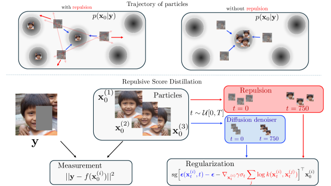
Figure 1: Illustrative figure of Repulsive score distillation for the case of inverse problems. Our method propagates a set of particles by gradually adding noise, and the applying two levels of regularization: the denoiser given by the score-matching regularization, which pushes towards one of the modes of the the distribution $p({\mathbf{x}}_{0}|{\mathbf{y}})$ (arrows in blue); and the repulsion, that repels the particles (arrows in red) in such a way that they explore other regions of the posterior density. During the sampling process via score distillation, the gradient associated to the repulsion term will keep particles away from each other, which allows to end up in different modes as it is shown in the box in the upper right.

All in all, the main contributions of this paper are summarized as follows:

1. We propose a framework for repulsive score distillation (RSD), a novel variational sampling that boosts diversity via interactive particle approximation of the gradient flow associated with KL divergence.

2. RSD leads to double regularization effect with simple and interpretable gradients: (1) a denoising regularization that effects quality, (2) a replusion regularization that promotes diversity. Thus, one can tune the trade-off by simply tuning the regularization weights.

3. As a byproduct, we extend RSD to inverse problems (constrained sampling) in the latent space, that not only promotes diversity but also solves the challenges associated with solving inverse problems in the latent space of diffusion models

4. Through extensive experiments with 2D text-to-image generation and inverse problems, we validate our method, striking a superior trade-off between diversity and quality compared with state of the arts

2 Related works

This paper is primarily related to two lines of work, in the context of diffusions for score distillation sampling, and inverse problems.

Score distillation: diversity and mode-collapse.

Recently, SDS was found successful for text-to-3D generation in DreamFusion [42] that suffers from mode collapse and saturated images due to the complex optimization landscape. ProlificDreamer [63], aims to fix the mode collapse using a data-drive dispersion, that is finetuned at each iteration via LoRA [23]. It is however costly and the particles do not seem to play role. Recently, the authors in [32] propose to use the well-known Stein variational gradient descent (SVGD) as an update direction, which yields an interactive particle system. However, it is known that SVGD suffers from the curse of dimensionality [10]. Other related works are [1], where the authors leverage the negative prompt to eliminate undesired perspectives, and [62], where an entropic regularization is proposed.

Diffusion models for inverse problems.

Several works have used diffusion models as priors to solve inverse problems in various domains [41, 5, 65, 33]. A recent approach uses variational inference for solving inverse problems with diffusion priors, similar to a plug-and-play method [41, 59]; see also [64, 16]. This method avoids likelihood approximation and employs the diffusion model as denoisers at different scales, akin to the RED framework [44]. Despite successfully balancing quality and runtime, it suffers from mode-collapse due to the unimodal approximation, which is problematic for sampling in high dimensions with multimodal posteriors. Moreover, pixel-domain optimization hinders leveraging models like Stable Diffusion [45]. It is thus still an open problem to develop methods that promote diversity and optimizing in the latent space of the diffusion model.

3 Background

3.1 Diffusion models in the latent space

Diffusion models [49, 20, 55] are composed of two processes: 1) a forward process that starts from a clean image and gradually adds noise; and 2) a reverse process that learns to generate images by iteratively denoising the diffused data. Formally, the forward process can be represented by several stochastic differential equations, the most commonly used being the variance-preserving stochastic differential equation (VP-SDE). When considering latent diffusion models, the diffusion is defined in a latent space. Namely, given a sample ${\mathbf{x}}_{0}$ from the data distribution, we encode it in the latent space through an encoder ${\mathcal{E}}({\mathbf{x}}_{0})={\mathbf{z}}_{0}$. Then, the VP-SDE is defined as $d{\mathbf{z}}_{t}=-\frac{1}{2}\beta(t){\mathbf{z}}_{t}\text{d}t+\sqrt{\beta(t)}\text{d}{\mathbf{W}}_{t}$, for $t\in[0,T]$. Here, $\beta(t)$ is a function that defines a step size for each $t$ from $0$ to $T$, and is defined as $\beta(t):=\beta_{\mathrm{min}}+(\beta_{\mathrm{max}}-\beta_{\mathrm{min}})\frac{t}{T}$, and ${\mathbf{W}}_{t}$ is the standard Brownian motion. The forward process is designed in such a way that the distribution of ${\mathbf{z}}_{T}$ converges to a standard Gaussian distribution. Given the forward process, the reverse process is defined as $d{\mathbf{z}}_{t}=-\frac{1}{2}\beta(t){\mathbf{z}}_{t}\text{d}t-\beta(t)\nabla_{{\mathbf{z}}_{t}}\log p({\mathbf{z}}_{t})+\sqrt{\beta(t)}\text{d}{\mathbf{W}}_{t}$, where $\nabla_{{\mathbf{z}}_{t}}\log p({\mathbf{z}}_{t})$ is the score function, which is unknown. To map back to the ambient space, we pass the generated sample ${\mathbf{z}}_{0}$ through a decoder ${\mathcal{D}}({\mathbf{z}}_{0})={\mathbf{x}}_{0}$. Therefore, to solve the reverse process and use it as a sampler, the score function ($\nabla_{{\mathbf{z}}_{t}}\log p({\mathbf{z}}_{t})$), the encoder (${\mathcal{E}}$), and the decoder (${\mathcal{D}}$) are learned by minimizing the denoising score-matching loss [60]. To do this, we first generate diffused samples as ${\mathbf{z}}_{t}=\alpha_{t}{\mathbf{z}}_{0}+\sigma_{t}\boldsymbol{\epsilon}$, where ${\mathbf{z}}_{0}$ is the encoding of ${\mathbf{x}}_{0}\sim p_{\mathrm{data}}({\mathbf{x}})$, a sample from the data distribution, and $\sigma_{t}=1-e^{-\int_{0}^{t}\beta(s)ds}$, and $\alpha_{t}=\sqrt{1-\sigma_{t}^{2}}$. Then, given a parametrization of the score function by $\boldsymbol{\epsilon}_{\boldsymbol{\theta}}({\mathbf{z}}_{t},t)\approx-\sigma_{t}\nabla_{{\mathbf{z}}_{t}}\log p({\mathbf{z}}_{t})$, we minimize the score-matching loss term; depending on the latent space [57, 45], different loss functions are defined. Once the score network is learned, we can generate samples by running different solvers, such as DDPM [20], DDIM [51], and others [12].

3.2 Score distillation and the gradient flow perspective

Consider a pretrained score function $\boldsymbol{\epsilon}_{\boldsymbol{\theta}}({\mathbf{x}}_{t},t)\approx-\sigma_{t}\nabla_{{\mathbf{x}}_{t}}\log p({\mathbf{x}}_{t})$ representing a distribution of interest $p_{\boldsymbol{\theta}}$. The idea of score distillation sampling (SDS) is to train a generator $g_{\boldsymbol{\phi}}$, such that the output of the generator given an input ${\mathbf{m}}$ is a sample ${\mathbf{x}}_{0}=g_{\boldsymbol{\phi}}({\mathbf{m}})\sim p_{\boldsymbol{\theta}}$. This is achieved by optimizing the distillation loss [42]

$${\mathcal{L}}_{\mathrm{SDS}}({\mathbf{x}}_{0}=g_{\boldsymbol{\phi}}(.))=\mathbb{E}_{t\sim{\mathcal{U}}[0,T],\boldsymbol{\epsilon}\sim{\mathcal{N}}(0,{\mathbf{I}})}\left[\omega(t)\frac{\sigma_{t}}{\alpha_{t}}D_{\mathrm{KL}}\left(q({\mathbf{x}}_{t}|{\mathbf{x}}_{0}=g_{\boldsymbol{\phi}}(.)\right)\mid\mid p_{\boldsymbol{\theta}}({\mathbf{x}}_{t}))\right],$$ (1)

where $\omega(t)$ is a weighting function, $q({\mathbf{x}}_{t}|{\mathbf{x}}_{0}=g_{\boldsymbol{\theta}}(.))$ is a variational distribution, and $D_{\mathrm{KL}}$ is the Kullback-Leibler (KL) divergence. Despite its remarkable success in generating 3D scenes [63], SDS suffers from mode collapse. This is mainly driven by the choice of the (reverse) KL divergence as the loss in (1) and the fact that a unimodal variational distribution $q$ is used.

It was recently shown [63] that SDS can be formulated as a Wasserstein gradient flow (WGF)

$$\mathrm{d}\mathbf{x}_{\tau}=\left(\nabla_{\mathbf{x}}\log p\left(\mathbf{x}_{\tau}\right)-\nabla_{\mathbf{x}}\log q_{\tau}\left(\mathbf{x}_{\tau}\right)\right)\mathrm{d}\tau,$$ (2)

where $p\left(\mathbf{x}_{\tau}\right)$ is the target distribution and $q_{\tau}\left(\mathbf{x}_{\tau}\right)$ is the variational distribution at time $\tau$; see Appendix B for a more in-depth discussion. We will leverage this alternative formulation to introduce our proposed method.

4 Repulsive score distillation

The key contribution in RDS to overcome the mode collapse limitation of SDS is to leverage ensemble methods to represent multi-modal variational distributions. Moreover, to achieve true multi-modality, we enhance these ensemble methods with a repulsion force that promotes mode exploration.

4.1 Approximating the WGF with an ensemble of particles

It is well-known [25] that the mean-field dynamics in (2) is intractable because of the marginal $q_{\tau}({\mathbf{x}}_{\tau})$. Therefore, we must resort to tractable (and simple) variational distributions or particle-based approximations; in this work, we focus on the latter. Particle-based methods, or ensemble methods, are popular techniques for approximating the gradient flow. In a nutshell, we approximate the distribution at each time step with an ensemble of $N$ particles, such that $q_{\tau}({\mathbf{x}}_{\tau})=\sum_{i=1}^{N}\delta({\mathbf{x}}_{\tau}-{\mathbf{x}}_{\tau}^{(i)})$. After enough time, the particles will approximate the target distribution. The accuracy of the approximation highly depends on the ability of the ensemble to explore the search space efficiently. A natural way to achieve this is by promoting diversity between the ensemble members. However, this can be challenging, especially when targeting high-dimensional multimodal distributions. Indeed, the ensemble will collapse to the same mode. This can be partially addressed in an ad hoc manner by changing the initial positions of the particles. By contrast, we propose a more principled approach: adding a repulsion term that prevents particles from collapsing into the same mode.

4.2 Repulsive force

Recall we seek a variational distribution that promotes diversity without compromising the accuracy of each generated image (see Figs. 2). Inspired by [11], we consider an ensemble of interacting particles coupled via a repulsive force that pushes particles away from collapsing to the same solution. In a nutshell, we introduce a repulsive force that yields the following modification of the gradient flow in (2)

$$\mathrm{d}\mathbf{x}_{\tau}^{(i)}=\left(\nabla_{\mathbf{x}^{(i)}}\log p\left(\mathbf{x}_{\tau}^{(i)}\right)-\nabla_{\mathbf{x}^{(i)}}\log q_{\tau}\left(\mathbf{x}^{(i)}_{\tau}\right)-\nabla_{{\mathbf{x}}^{(i)}}{\mathcal{R}}({\mathbf{x}}_{\tau}^{(1)},\cdots,{\mathbf{x}}_{\tau}^{(N)})\right)\mathrm{d}\tau,\quad i=1,\cdots,N,$$ (3)

where ${\mathcal{R}}({\mathbf{x}}_{\tau}^{(1)},\cdots,{\mathbf{x}}_{\tau}^{(N)})$ is the coupling between particles such that its gradient is the repulsive force. Notice that the marginal distribution in (3) at each time step $\tau$ is given by (where $Z$ is a normalizing constant)

$$q_{\tau}({\mathbf{x}}_{\tau}^{(1)},\cdots,{\mathbf{x}}_{\tau}^{(N)})=\frac{1}{Z}{\mathcal{R}}({\mathbf{x}}_{\tau}^{(1)},\cdots,{\mathbf{x}}_{\tau}^{(N)})\prod_{i=1}^{N}q_{\tau}({\mathbf{x}}_{\tau}^{(i)}).$$ (4)

Throughout this work, we consider a pairwise kernel function $k$ such that the repulsive force adopts the form $\nabla_{{\mathbf{x}}^{(i)}}{\mathcal{R}}({\mathbf{x}}_{\tau}^{(1)},\cdots,{\mathbf{x}}_{\tau}^{(N)})=\nabla_{{\mathbf{x}}^{(i)}}\sum_{j=1}^{N}\log k\left({\mathbf{x}}_{\tau}^{(i)},{\mathbf{x}}_{\tau}^{(j)}\right)^{\gamma}$; see the numerical experiments for the particular instances of the kernel $k$. The repulsive force allows us to consider simple and flexible variational distributions that can discover multiple modes. For a simple illustration in the Gaussian case, see Appendix C.3.1. Finally, notice that when $\gamma=0$, we recover the i.i.d. (non-repulsive) case.

Comparison with SVGD.

Our proposed gradient flow in (3) might be reminiscent of SVGD [38]. However, there are two fundamental differences: i) the second term in the RHS of (3) is not present in SVGD, and ii) the first term (the gradient of the log target distribution) is replaced by a weighted sum over all the particles. This difference in the score has important implications: the directions of the particles are more similar to each other in SVGD than in our proposed update. Consequently, SVGD shows poor exploration of the space in high-dimensional multimodal distributions and suffers from mode collapse. A formal comparison is deferred to Appendix B.4.

4.3 Score distillation meets repulsive ensemble methods

We now leverage the WGF perspective of SDS to derive an optimization procedure that promotes diversity using a repulsive force. Our objective is to train the parameters of a generator such that the output matches some target object, namely a 3D scene or a clean image in inverse problems. Formally, we consider a generator $g_{\boldsymbol{\phi}}({\mathbf{m}})$ where $\boldsymbol{\phi}$ are random variables distributed as $\mu(\boldsymbol{\phi}|{\mathbf{y}})$, ${\mathbf{m}}$ is some domain-dependent input, and ${\mathbf{y}}$ is some task-dependent variable (such as a prompt or a noisy measurement). Then, for a given $\boldsymbol{\phi}$, ${\mathbf{m}}$ and ${\mathbf{y}}$, we have a clean rendered image ${\mathbf{x}}_{0}=g_{\boldsymbol{\phi}}({\mathbf{m}})$ related to ${\mathbf{y}}$, which can be diffused to noise level $t$ such that ${\mathbf{x}}_{t}=\alpha_{t}g_{\boldsymbol{\phi}}({\mathbf{m}})+\sigma_{t}\boldsymbol{\epsilon}_{t}$. Given these ingredients, we obtain the distribution of the parameters of the generator by solving the following optimization problem in (5)

$$\mu(\boldsymbol{\phi}|{\mathbf{y}})=\operatornamewithlimits{argmin}_{\mu(\boldsymbol{\phi}|{\mathbf{y}})}\mathrm{KL}(q({\mathbf{x}}_{0}|{\mathbf{y}},\boldsymbol{\phi})\mid\mid p({\mathbf{x}}_{0}|{\mathbf{y}})).$$ (5)

Following [54], we can rewrite the above equation in terms of the diffused trajectory as

$$\mu(\boldsymbol{\phi}|{\mathbf{y}})=\operatornamewithlimits{argmin}_{\mu(\boldsymbol{\phi}\mid{\mathbf{y}})}\mathbb{E}_{t,\epsilon}\left[\omega(t)\mathrm{KL}(q({\mathbf{x}}_{t}|{\mathbf{y}},\boldsymbol{\phi})\mid\mid p_{\boldsymbol{\theta}}({\mathbf{x}}_{t}|{\mathbf{y}}))\right],$$ (6)

where $q({\mathbf{x}}_{t}|{\mathbf{y}},\boldsymbol{\phi})=\int q({\mathbf{x}}_{t}|{\mathbf{x}}_{0})q({\mathbf{x}}_{0}|{\mathbf{y}},\boldsymbol{\phi})\text{d}{\mathbf{x}}_{0}$. The optimization defined in (6) can be reformulated as a WGF in the space of measures. This was formalized in Theorem 2 in [63] (for completeness, we reproduce this theorem in Appendix B.3). The associated WGF entails a dynamical system at the particle level described by

$$\mathrm{d}\boldsymbol{\phi}_{\tau}=\mathbb{E}_{t,\epsilon,{\mathbf{m}}}\left[\omega(t)\left(\nabla_{{\mathbf{x}}_{t,\tau}}\log p\left(\mathbf{x}_{t,\tau}\mid{\mathbf{y}}\right)-\nabla_{\mathbf{x}_{t,\tau}}\log q_{t,\tau}\left(\mathbf{x}_{t,\tau}\mid{\mathbf{y}},\boldsymbol{\phi}_{\tau},{\mathbf{m}}\right)\right)\frac{\partial\boldsymbol{g}_{\boldsymbol{\phi}_{\tau}}({\mathbf{m}})}{\partial\boldsymbol{\phi}_{\tau}}\right]\mathrm{d}\tau.$$ (7)

Consequently, we can generate samples from the target distribution $\mu(\boldsymbol{\phi}|{\mathbf{y}})$ by running (7), which requires access to the score of noisy real images given the input ${\mathbf{y}}$ and the score of the noisy rendered images. Notice that the main difference with the definition in (2) is that here we are using gradient information in a different domain than the particles; in other words, we are distilling the information of the pre-trained score of images to train the generator.

Unconstrained sampling.

When the input ${\mathbf{y}}$ is a prompt, denoted as ${\mathbf{y}}=c$, then we are in the unconstrained case, and therefore, we can use a pre-trained model to approximate the score of noisy real images, i.e., the first gradient in (7) (for the conditional case, see Section 5). Regarding the second gradient, we propose to approximate it with the repulsive distribution in (4) with N interacting particles. In this case, for each particle $i$, we have the dynamics in (7), but where the second gradient is replaced by

$$\nabla_{{\mathbf{x}}_{t,\tau}^{(i)}}\sum_{j=1}^{N}\log k\left({\mathbf{x}}_{t,\tau}^{(i)},{\mathbf{x}}_{t,\tau}^{(j)}\right)^{\gamma}+\nabla_{{\mathbf{x}}_{t,\tau}^{(i)}}\log q_{t,\tau}({\mathbf{x}}_{t,\tau}^{(i)}\mid c,\boldsymbol{\phi}_{\tau}^{(i)},{\mathbf{m}}),$$ (8)

where the first term encodes the repulsive force between the images. Each rendered image ${\mathbf{x}}_{t}^{(i)}$ is associated with a parameter $\boldsymbol{\phi}^{(i)}$. Importantly, our method does not specify a particular choice for the gradient of each individual particle (second term in (8)); in Section 6 we demonstrate that our method is agnostic to this selection and promotes diversity independently of the chosen method. The algorithm of RSD is shown in Alg. 1 in Appendix C.

5 Constrained sampling: Solving inverse problems

The approach in Section 4.3 can also be used when ${\mathbf{y}}$ is a noisy measurement of some unknown image, giving rise to an inverse problem. In this setting, however, we no longer optimize over a distribution of the generator parameters $\phi$ but rather over the distribution $q({\mathbf{x}}_{0}\mid{\mathbf{y}})$ directly. This is, indeed, a particular case of (5) where the generator $g_{\phi}(\cdot)=\phi$ is the identity. For inverse problems, we advocate the use of a suitable latent space. More precisely, assuming access to a pre-trained latent diffusion model, we can solve the inverse problem by minimizing (5) in the latent space ${\mathbf{z}}$ and then mapping to the pixel domain; this approach was proposed recently in a method termed RED-diff [41]. This formulation assumes a Gaussian distribution $q({\mathbf{z}}_{0}|{\mathbf{y}})\sim{\mathcal{N}}(\boldsymbol{\mu}_{z},\boldsymbol{\sigma}_{z}^{2}{\mathbf{I}})$. Then, the KL minimization boils down to a MAP optimization algorithm that leverages the trajectory generated by the diffusion model as a regularizer. Although this approach seems a natural adaptation of RED-diff to handle latent diffusion models, the estimated images that we obtain are blurry (see Appendix D.3). In the following sections, we propose an alternative approach to circumvent this issue.

5.1 Diffusion models for inverse problems.

In general, an inverse problem aims to find an unknown signal ${\mathbf{x}}_{0}$ given some noisy measurement ${\mathbf{y}}$, related via some forward model $f(.)$,

$${\mathbf{y}}=f({\mathbf{x}}_{0})+{\mathbf{v}},\quad{\mathbf{v}}\sim{\mathcal{N}}(0,\sigma_{v}^{2}{\mathbf{I}}),$$ (9)

where the forward model is domain-dependent. When considering a diffusion model as prior, we need to run the reverse process (see Section 3.1) by following the conditional score at $t$ obtained via Bayes’ rule as

$$\nabla_{{\mathbf{x}}_{t}}\log p({\mathbf{x}}_{t}|{\mathbf{y}})=\nabla_{{\mathbf{x}}_{t}}\log p({\mathbf{y}}|{\mathbf{x}}_{t})+\nabla_{{\mathbf{x}}_{t}}\log p({\mathbf{x}}_{t}).$$ (10)

While the second term is obtained from a pre-trained diffusion model, the first one is intractable; this can be seen from the fact that $p({\mathbf{y}}|{\mathbf{x}}_{t})=\int p({\mathbf{y}}|{\mathbf{x}}_{0})p({\mathbf{x}}_{0}|{\mathbf{x}}_{t})\text{d}{\mathbf{x}}_{0}$. Prior works [5, 52, 26, 53] circumvent this by considering a Gaussian approximation of $p({\mathbf{x}}_{0}|{\mathbf{x}}_{t})$ centered at the MMSE estimator, obtained via Tweedie’s formula $\mathbb{E}[{\mathbf{x}}_{0}|{\mathbf{x}}_{t}]=\frac{1}{\alpha_{t}}\left({\mathbf{x}}_{t}-\sigma_{t}\epsilon({\mathbf{x}}_{t},t)\right)$. This approach requires backpropagation through the score network, which can be computationally expensive.

5.1.1 Augmentation of the variational distribution

We propose an augmented version of the variational formulation in (5), allowing us to decouple the data and the latent space of the diffusion model. Formally, we introduce an auxiliary variable ${\mathbf{x}}_{0}$ defined in the pixel space, which entails an augmented variational distribution $q({\mathbf{z}}_{0},{\mathbf{x}}_{0}|{\mathbf{y}})$ and an augmented posterior as

$$p({\mathbf{z}}_{0},{\mathbf{x}}_{0}|{\mathbf{y}})\propto\exp\left(-\frac{1}{2\sigma_{v}^{2}}||{\mathbf{y}}-f({\mathbf{x}}_{0})||^{2}-\lambda g({\mathbf{z}}_{0})-\frac{1}{2\rho^{2}}||{\mathbf{x}}_{0}-{\mathcal{D}}({\mathbf{z}}_{0})||^{2}\right),$$ (11)

where $\rho$ controls the correlation between the variables ${\mathbf{x}}_{0}$ and ${\mathbf{z}}_{0}$. It can be shown that $p({\mathbf{x}}_{0}|{\mathbf{y}},\lambda,\rho^{2})$ converges in total variational to the true posterior $p({\mathbf{x}}_{0}|{\mathbf{y}},\lambda)$ when $\rho\rightarrow 0$ [58, 61] (details can be found in Appendix A.1). Now, we can reformulate our optimization problem as

$$q({\mathbf{z}}_{0},{\mathbf{x}}_{0}|{\mathbf{y}})=\operatornamewithlimits{argmin}_{q({\mathbf{z}}_{0},{\mathbf{x}}_{0}|{\mathbf{y}})}\mathrm{KL}(q({\mathbf{z}}_{0},{\mathbf{x}}_{0}|{\mathbf{y}})\|p({\mathbf{z}}_{0},{\mathbf{x}}_{0}|{\mathbf{y}})).$$ (12)

When considering a diffusion model as data prior, our problem boils down to minimizing the variational lower bound, formalized in Proposition 1

Proposition 1

Assuming we have access to a diffusion model $\nabla_{{\mathbf{z}}_{t}}\log p\left({\mathbf{z}}_{t}\right)$ for the prior on ${\mathbf{z}}_{0}$, then the KL minimization w.r.t q in (12) is equivalent to minimizing the variational bound, that itself obeys the following update rule

$$\min_{q({\mathbf{x}}_{0},{\mathbf{z}}_{0}|{\mathbf{y}})}\mathbb{E}_{q({\mathbf{z}}_{0}|{\mathbf{y}})}[H(q({\mathbf{x}}_{0}|{\mathbf{z}}_{0},{\mathbf{y}}))]+\mathbb{E}_{q({\mathbf{x}}_{0},{\mathbf{z}}_{0}|{\mathbf{y}})}\left[\frac{1}{2\sigma_{v}^{2}}\|{\mathbf{y}}-f({\mathbf{x}}_{0})\|^{2}\right]$$ (13)

$$+\mathbb{E}_{q({\mathbf{x}}_{0},{\mathbf{z}}_{0}|{\mathbf{y}})}\left[\frac{1}{2\rho^{2}}\|{\mathbf{x}}_{0}-{\mathcal{D}}({\mathbf{z}}_{0})\|^{2}\right]+\int_{0}^{T}\tilde{\omega}(t)\mathbb{E}_{q\left({\mathbf{z}}_{t}\mid{\mathbf{y}}\right)}\left[\left\|\nabla_{{\mathbf{z}}_{t}}\log q\left({\mathbf{z}}_{t}\mid{\mathbf{y}}\right)-\nabla_{{\mathbf{z}}_{t}}\log p\left({\mathbf{z}}_{t}\right)\right\|_{2}^{2}\right]dt.$$

The proof is in Appendix A.2. When $\rho\rightarrow 0$, then ${\mathbf{x}}_{0}={\mathcal{D}}({\mathbf{z}}_{0})$ and the augmented KL optimization boils down to the objective in [41]. To solve the problem in Proposition 1, we need to specify the variational distribution $q({\mathbf{x}}_{0},{\mathbf{z}}_{0}|{\mathbf{y}})$.

5.1.2 Repulsive score distillation for solving inverse problems

We define a specific case of the problem outlined in Proposition 1 by considering a repulsive variational distribution. Previous works have typically used unimodal approximations of either the score posterior [5] or the variational distribution to approximate the multimodal posterior [41]. To overcome this limitation, we utilize the particle approximation defined in (4), which enables more thorough exploration and the discovery of multiple modes. The update rule is defined in Proposition 2

Proposition 2

When considering the variational distribution defined in (4), the KL minimization w.r.t $q({\mathbf{x}}_{0},{\mathbf{z}}_{0}|{\mathbf{y}})$ defined in Proposition 1 can be approximated with an ensemble of $N$ particles that are optimized using the following update rule

$$\frac{1}{N}\sum_{i=1}^{N}\nabla_{{\mathbf{u}}^{(i)}}\left[\|{\mathbf{y}}-f({\mathbf{x}}_{0}^{(i)})\|^{2}+\|{\mathbf{x}}_{0}^{(i)}-{\mathcal{D}}({\mathbf{z}}_{0}^{(i)})\|^{2}\right]+\nabla_{{\mathbf{z}}_{0,\tau}^{(i)}}\mathrm{reg}({\mathbf{z}}_{t,\tau}^{(1)},\cdots,{\mathbf{z}}_{t,\tau}^{(N)})$$ (14)

for $i=1,\cdots,N$ and where ${\mathbf{u}}^{(i)}=[{\mathbf{x}}_{0}^{(i)},{\mathbf{z}}_{0}^{(i)}]$. The regularization term is given by

$$\nabla_{{\mathbf{z}}_{0,\tau}^{(i)}}\mathrm{reg}({\mathbf{z}}_{t,\tau}^{(1)},\cdots,{\mathbf{z}}_{t,\tau}^{(N)})=\mathbb{E}_{\boldsymbol{\epsilon},t}\left[\lambda_{t}\left(\epsilon({\mathbf{z}}_{t,\tau}^{(i)},t)-\boldsymbol{\epsilon}-\nabla_{{\mathbf{z}}_{t,\tau}^{(i)}}\gamma\sigma_{t}\log\sum_{j=1}^{N}k\left({\mathbf{z}}_{t,\tau}^{(i)},{\mathbf{z}}_{t,\tau}^{(j)}\right)\right)\right].$$ (15)

where $\lambda_{t}:=\frac{4T\sigma_{v}^{2}\rho^{2}\alpha_{t}}{\sigma_{t}}\frac{\text{d}\omega(t)}{\text{d}t}$ and $\gamma\geq 0$.

Proof can be found in Appendix A.3. The update rule defined in Proposition 2 comprises three terms: a measurement matching term, an error term measuring the discrepancy between the variable in the ambient space and the augmented variable post-decoder, and a final term that combines a score-matching regularizer with a diversity-promoting component. This repulsion term acts as a second regularizer, enhancing diversity in the sampling process. Our approach is not limited to any specific latent diffusion model.

Optimization of latent RED-diff with repulsion.

Notice that the optimization problem in Proposition 1 is highly non-convex (diffusion denoiser and the repulsion term) and difficult to solve. We adopt a half quadratic splitting technique [15]. The algorithm is shown in Algo 2 in Appendix D. For the weighting function $\lambda_{t}$ ($\omega(t)$ is embedded), we follow the strategy introduced in [41], where $\lambda_{t}=\lambda(\sigma_{t}/\alpha_{t})=\lambda/\mathrm{SNR}_{t}$.

6 Experiments

6.1 Unconstrained sampling: text-to-image generation

In this section, we compare RSD against state-of-the-art distillation techniques in text-to-image generation. Recall our goal is to promote diversity in the generation of images while keeping the quality in check. Therefore, throughout the following experiments, we seek to answer: 1) Does our method promote image diversity? 2) What is the trade-off between diversity and quality?

Setup of our method.

In the following experiments, we consider ProlificDreamer as our distillation baseline, i.e., we use ProlificDreamer for our second term in (8). For ProlificDreamer uses Stable diffusion 2.1 trained in the LAION dataset as its pre-trained model. Details of the hyperparameters can be found in Appendix C.1. We use the filtered version from the COCO validation set [36] constructed in [24]. For the kernel function, we consider a RBF $k({\mathbf{z}}_{i},{\mathbf{z}}_{j})=\exp(-\frac{||g_{\text{DINO}}({\mathbf{z}}_{i})-g_{\text{DINO}}({\mathbf{z}}_{j})||^{2}}{h_{t}})$ where $h_{t}=m_{t}^{2}/\log N$, $m_{t}$ is the median particle distance [38] and $g_{\text{DINO}}$ is a pre-trained neural network [3]. As metrics, we evaluate the pairwise similarity as the cosine similarity (37) between the N particles for a given prompt $c$. For quality, we consider the FID between the generated images and the complete COCO validation set, the Aesthetic score [56], and the CLIP score [18]. An ablation study can be found in Appendix C.2.

6.1.1 2D image generation

In this first subsection, we optimize directly in the latent space of the diffusion model. Specifically, we use an identity generator $g_{\boldsymbol{\phi}}(.)=\boldsymbol{\phi}$, which is initialized at random. In Fig. 2, we compare the generated images using ProlificDremer with and without repulsion. Recall that the ‘no repulsion’ method can be obtained by setting $\gamma=0$ in (8). We observe that, in both cases, the repulsion yields more image diversity (as quantified by the pairwise similarities) while the quality of images is not affected. More visual results, including comparisons with Noise-free Score distillation (NFSD) [28], are shown in Appendix C.3.

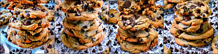
(a) ProlificDreamer

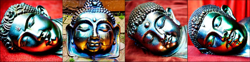
(b) ProlificDreamer

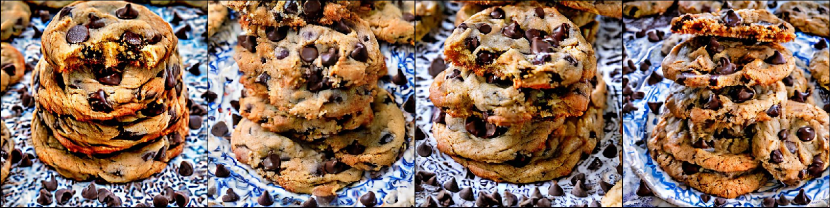
(c) ProlificDreamer with repulsion

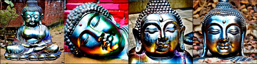
(d) ProlificDreamer with repulsion

Figure 2: a, c) Generated samples using the prompt "A plate piled high with chocolate chip cookies". a) ProlificDreamer with a pairwise similarity of 0.86, c) Prolific Dreamer with repulsion and a pairwise similarity of 0.75 ($\gamma=20$). b, d) Generated samples using the prompt "A metal lying Buddah". b) ProlificDreamer with a pairwise similarity of 0.67, d) ProlificDreamer with repulsion with a pairwise similarity of 0.58 ($\gamma=10$). We observe empirically that adding repulsion yields a more diverse set of images while keeping a good visual quality.

6.1.2 Trade-off between diversity and quality

Motivated by the previous experiment, we study the trade-off between diversity and quality when increasing the amount of repulsion. We consider 75 images from the COCO dataset and compute average qualities and diversities across all images. We also include a comparison with stochastic sampling using the Euler discretization of the backward process, with 30 steps (denoted by ‘Ancestral’). This serves as an upper bound on the performance of distillation techniques. We consider 4 particles for both the distillation optimization and the sampling via Euler. The results are shown in Fig. 3, where we compute FID (lower is better), Aesthetic (higher is better) and CLIP (higher is better) scores as a function of a diversity score (defined as $1$ minus the average pairwise similarity between the images associated with the same prompt; see Appendix C.1). A higher diversity score corresponds to more diverse image generation. For the plot, we fix all the hyperparameters, and we sweep $\gamma$ between 0 (ProlificDreamer) and 40, and we consider Ancestral sampling as an upper bound in terms of trade-off. Clearly, adding repulsion increases the diversity, while slightly decreasing the quality metrics for low values of $\gamma$. However, for these lower values of $\gamma$, the diversity is still far from the stochastic sampling. When increasing the values of $\gamma$ above 30, we close the gap in terms of diversity at the cost of decreasing the quality (FID and Aesthetic) as well as the text-alignment (CLIP). Appendix C.3.3 shows some images used to construct these curves. Also, for completeness, in Appendix C.3.2 we show trade-off plots with the corresponding standard deviations, where we also include SDS.

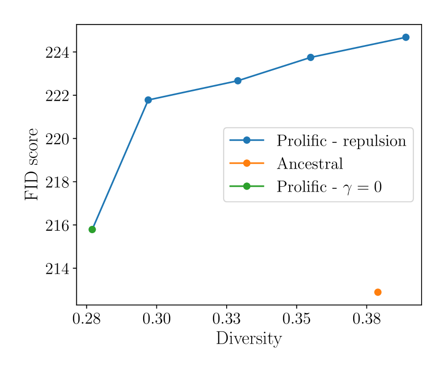
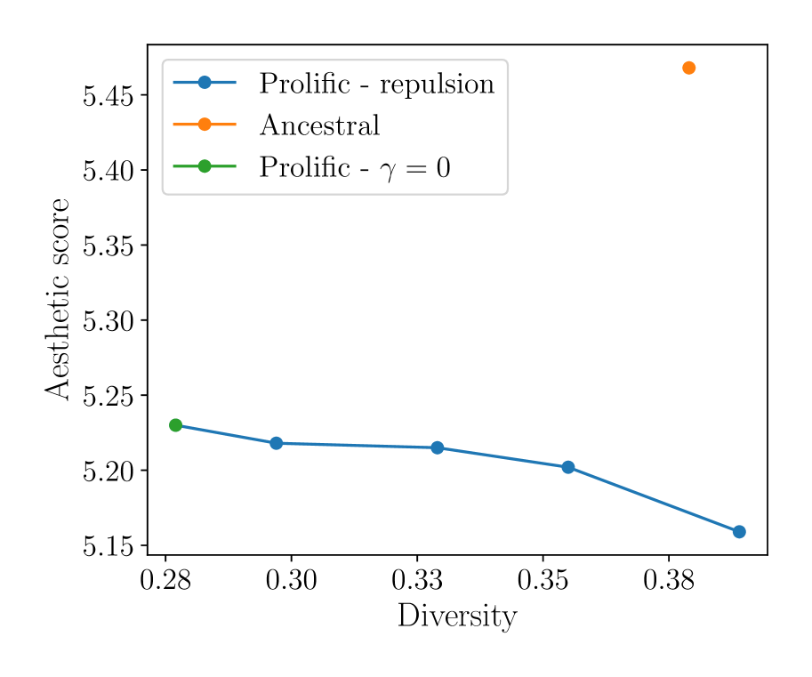
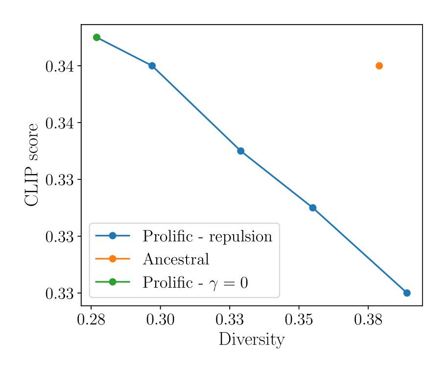
Figure 3: We consider the trade-off between diversity and quality for text-to-2D image generation using score distillation. We consider $\gamma=\{0,10,20,30,40\}$. From left to right: Diversity (38) vs left) FID, middle) Aesthetic score and right) CLIP score. We consistently observe that adding repulsion increases diversity, while slightly decreasing the quality of the images. Notice that we need a repulsion with $\gamma>30$ to reach the diversity level of stochastic sampling using Euler.

6.1.3 Text-to-3D generation

Lastly, we test our repulsion method for text-to-3D generation. Our main motivation is to show that including the repulsion entails a more diverse set of scenes when changing the seed. We consider DreamFusion [42] as base method and the implementation from the Threestudio framework [17]. All 3D models are optimized for 10000 iterations using Adam optimizer with a learning rate of 0.01, and we use the same configuration as DreamFusion for the rendering. We consider a batch of 20 particles for all the experiments; this presents a limitation for using more computationally-demand methods such as ProlificDreamer.

In Fig. 4 we show a qualitative example; we deferred to Appendix C.3.5 for more experiments with other prompts. For each case, we show two different views of the generated object. Notice that with repulsion we can generate two different colors of glass for the ice cream (dark and white), something that we could not achieve without repulsion. Furthermore, while the case without repulsion generates two scenes that have a similar perspective, our method generates two scenes that show the ice cream at different distances. Lastly, notice that the quality of the generated scene is bounded by the performance of the base method (in this case, DreamFusion). Therefore, the results look saturated, similar to what happen with SDS.

6.2 Inverse problems

In this section, we compare our proposed method with repulsion against state-of-the-art algorithms for solving inverse problems using latent diffusion models. The setup for the experiment can be found in Appendix D.2 We consider the first 100 samples from the validation set of 1k samples of FFHQ [27] used in [5]. We compute PSNR [dB], LPIPS, and FID as metrics.

Baselines methods.

As we focus on methods that leverage large pre-trained model such as Stable diffusion, we compare with the recent PSLD [46], and RED-diff [41] defined in the latent space. For PSLD, we run the experiments using the setup from the paper’s repository. For completeness, we include in the appendix a comparison with SOTA method in the pixel-domain, namely DPS [5] and RED-diff [41].

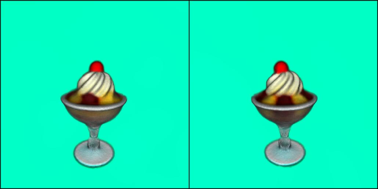
(a) Without repulsion - Seed 0

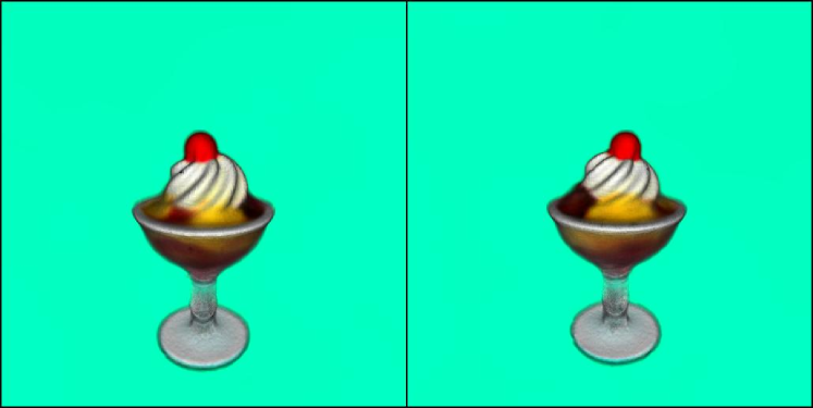
(b) Without repulsion - Seed 15

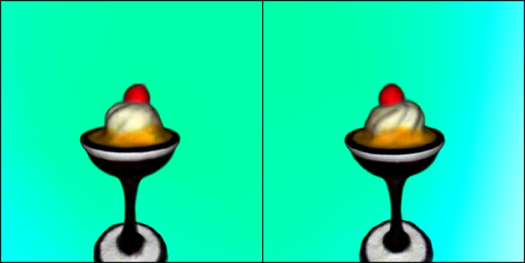
(c) With repulsion - Seed 0

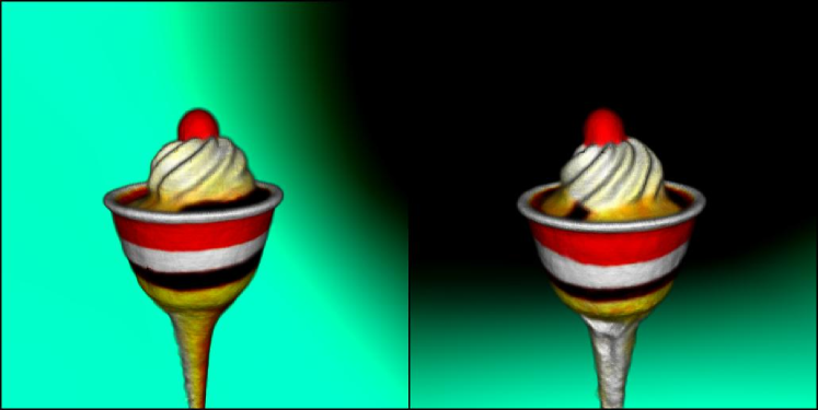
(d) With repulsion - Seed 15

Figure 4: Text-to-3D generation using DreamFusion with the prompt "An ice cream sundae", and considering a batch of 20 samples (particles) a, b) without repulsion with seed 0 and seed 15, c, d) with repulsion with seed 0 and 15 respectively. For each case, we show two different views of the object. Clearly, the two cases without repulsion look very similar, generating the same type of ice cream sundae. On the other hand, adding repulsion increase diversity of the scene (a different glass, and color). However, this comes at the cost of less details in the ice cream.

6.2.1 Inpainting

We focus on inpainting to demonstrate two key aspects of our method: 1) high-quality reconstruction and 2) increased diversity with the repulsion term. Inpainting, with its inherent ambiguity, is a suitable benchmark. Additional inverse problems are detailed in Appendix D. Specifically, we consider a box hiding half of the faces; see figures in Appendix D.4.1. Results in Table 1 show that RSD (with repulsion) achieves higher diversity than the case without repulsion, and slightly less than PSLD, while the non-repulsion case ($\gamma=0$) outperforms the baselines in image quality for two metrics. This highlights RSD’s ability to combine superior reconstruction with higher diversity, suggesting a mixed strategy where some particles interact and others do not.

Table 1: Box inpainting (half face) with $\sigma_{v}=0.001$. The best method for each metric and experiment is bolded.

Method	PSNR [dB] $\uparrow$	LPIPS $\downarrow$	FID $\downarrow$	Diversity
PSLD	21.33	0.126	57.7	0.03
Latent RED-diff	22.13	0.307	92.59	0.03
RSD ($\gamma=0$)	24.98	0.109	29.18	0.004
RSD ($\gamma=50$)	24.69	0.111	31.41	0.015

7 Conclusions and limitations

This paper introduces Repulsive Score Distillation (RSD) to address mode collapse in score distillation techniques. RSD promotes diversity in generated images without significantly compromising quality by using a repulsive regularizer that allows ensemble particles to interact. Our method is plug-and-play, and integrates seamlessly with other techniques. We also derive a variational sampler leveraging large pre-trained diffusion models to solve inverse problems, optimizing an augmented variational distribution with two regularizations: the diffusion process for multi-scale regularization and a repulsion term for diversity. We demonstrate through numerical experiments that the repulsion force enhances diversity in both unconstrained (text-to-image) and constrained (inverse problems) contexts.

Our work presents limitations that we plan to address. The increased computational demand due to the repulsion term poses challenges for real-time applications. Moreover, the chosen repulsion kernel may not be optimal, particularly for higher noise levels in the diffusion process, suggesting exploration of adaptive kernel learning. Additionally, our formulation of the variational sampler for inverse problems introduces more hyperparameters, warranting investigation into better couplings to handle noise levels and deriving a repulsion weight based on the forward operator’s characteristics. Finally, the results for each experiment are bounded by the base method that we use; in particular, in text-to-3D the results look saturated. We leave as future work an implementation of RSD with base method that generates more realistic scenes.

Appendix A Technical proofs

A.1 Data augmentation

In Section 5.1.1 we consider an augmented variational distribution $q_{\rho}({\mathbf{x}}_{0},{\mathbf{z}}_{0}|{\mathbf{y}})$ such that

$$q_{\rho}({\mathbf{x}}_{0}|{\mathbf{y}})=\int q_{\rho}({\mathbf{x}}_{0},{\mathbf{z}}_{0}|{\mathbf{y}})\text{d}{\mathbf{z}}_{0}.$$ (16)

Therefore, we seek a joint distribution such that Property 1 holds.

Property 1

For all ${\mathbf{x}}_{0}\in{\mathbb{R}}^{N}$, it holds $\lim_{\rho\rightarrow 0}\pi_{\rho}({\mathbf{x}}_{0})=\pi({\mathbf{x}}_{0})$.

Notice that our approach using data augmentation resembles some recent methods introduced in the bibliography. In [64] the authors propose, More recently, a Bayesian version of the RED method was proposed in [14]. This method shares a similarities with our method, in the sense that both are augmented versions that resembles RED. However, our method has three main differences: 1) it leverage latent diffusion models, which allows to solve large-scale inverse problems ($512\times 512$ and beyond), 2) it uses the diffused trajectory to regularize the solution, and 3) it promotes diversity via the coupling term.

A.2 Proof of proposition 1

We expand the KL objective as follow

$$\mathrm{KL}(q({\mathbf{z}}_{0},{\mathbf{x}}_{0}|{\mathbf{y}})\|p({\mathbf{z}}_{0},{\mathbf{x}}_{0}|{\mathbf{y}})) =\int q({\mathbf{z}}_{0},{\mathbf{x}}_{0}|{\mathbf{y}})\log\frac{q({\mathbf{z}}_{0},{\mathbf{x}}_{0}|{\mathbf{y}})}{p({\mathbf{z}}_{0},{\mathbf{x}}_{0}|{\mathbf{y}})}\text{d}{\mathbf{z}}_{0}\text{d}{\mathbf{x}}_{0}$$ (17)

$$=\int q({\mathbf{z}}_{0},{\mathbf{x}}_{0}|{\mathbf{y}})\log\frac{q({\mathbf{x}}_{0}|{\mathbf{z}}_{0},{\mathbf{y}})q({\mathbf{z}}_{0}|{\mathbf{y}})p({\mathbf{y}})}{p({\mathbf{y}}\mid{\mathbf{x}}_{0})p({\mathbf{x}}_{0}|{\mathbf{z}}_{0})p({\mathbf{z}}_{0})}\text{d}{\mathbf{z}}_{0}\text{d}{\mathbf{x}}_{0}$$

$$=\underbrace{\int q({\mathbf{z}}_{0},{\mathbf{x}}_{0}|{\mathbf{y}})\log q({\mathbf{x}}_{0}|{\mathbf{z}}_{0},{\mathbf{y}})\text{d}{\mathbf{z}}_{0}\text{d}{\mathbf{x}}_{0}}_{(i)}$$

$$-\underbrace{\int q({\mathbf{z}}_{0},{\mathbf{x}}_{0}|{\mathbf{y}})\log p({\mathbf{y}}\mid{\mathbf{x}}_{0})\text{d}{\mathbf{z}}_{0}\text{d}{\mathbf{x}}_{0}}_{(ii)}$$

$$-\int\underbrace{q({\mathbf{z}}_{0},{\mathbf{x}}_{0}|{\mathbf{y}})\log p({\mathbf{x}}_{0}|{\mathbf{z}}_{0})\text{d}{\mathbf{z}}_{0}\text{d}{\mathbf{x}}_{0}}_{(iii)}$$

$$+\underbrace{\int q({\mathbf{z}}_{0},{\mathbf{x}}_{0}|{\mathbf{y}})\frac{q({\mathbf{z}}_{0}|{\mathbf{y}})}{p({\mathbf{z}}_{0})}\text{d}{\mathbf{z}}_{0}\text{d}{\mathbf{x}}_{0}}_{(iv)}+\log p({\mathbf{y}}).$$

Based on the augmented posterior, we have for $(ii)$ and $(iii)$ that

$$(ii)=\int q({\mathbf{z}}_{0},{\mathbf{x}}_{0}|{\mathbf{y}})\log p({\mathbf{y}}\mid{\mathbf{x}}_{0})\text{d}{\mathbf{z}}_{0}\text{d}{\mathbf{x}}_{0}=\mathbb{E}_{q({\mathbf{x}}_{0},{\mathbf{z}}_{0}|{\mathbf{y}})}\left[\frac{1}{2\sigma_{v}^{2}}\|{\mathbf{y}}-f({\mathbf{x}}_{0})\|^{2}\right]$$ (18)

and

$$(iii)=\int q({\mathbf{z}}_{0},{\mathbf{x}}_{0}|{\mathbf{y}})\log p({\mathbf{x}}_{0}\mid{\mathbf{z}}_{0})\text{d}{\mathbf{z}}_{0}\text{d}{\mathbf{x}}_{0}=\mathbb{E}_{q({\mathbf{x}}_{0},{\mathbf{z}}_{0}|{\mathbf{y}})}\left[\frac{1}{2\rho^{2}}\|{\mathbf{x}}_{0}-{\mathcal{D}}({\mathbf{z}}_{0})\|^{2}\right].$$ (19)

Regarding the first term, we can write as

$$(i)=\int q({\mathbf{z}}_{0}|{\mathbf{y}})\left[q({\mathbf{x}}_{0}\mid{\mathbf{z}}_{0},{\mathbf{y}})\log q({\mathbf{x}}_{0}|{\mathbf{z}}_{0},{\mathbf{y}})\right]\text{d}{\mathbf{z}}_{0}\text{d}{\mathbf{x}}_{0}=\mathbb{E}_{q({\mathbf{z}}_{0}\mid{\mathbf{y}})}\left[H(q({\mathbf{x}}_{0}\mid{\mathbf{z}}_{0},{\mathbf{y}})\right].$$ (20)

Finally, the last term can be obtained by following theorem 2 in [54], assuming that the score is learned exactly, namely $\epsilon_{\theta}\left({\mathbf{z}}_{t};t\right)=$ $-\sigma_{t}\nabla_{{\mathbf{z}}_{t}}\log p\left({\mathbf{z}}_{t}\right)$, and under some mild assumptions on the growth of $\log q\left({\mathbf{z}}_{t}\mid{\mathbf{y}}\right)$ and $p\left({\mathbf{z}}_{t}\right)$ at infinity, we have

$$\mathrm{KL}(q({\mathbf{z}}_{0}|{\mathbf{y}})\|p({\mathbf{z}}_{0}))=\int_{0}^{T}\frac{\beta(t)}{2}\omega(t)\mathbb{E}_{q\left({\mathbf{z}}_{t}\mid{\mathbf{y}}\right)}\left[\left\|\nabla_{{\mathbf{z}}_{t}}\log q\left({\mathbf{z}}_{t}\mid{\mathbf{y}}\right)-\nabla_{{\mathbf{z}}_{t}}\log p\left({\mathbf{z}}_{t}\right)\right\|_{2}^{2}\right]dt$$ (21)

over the denoising diffusion trajectory $\left\{{\mathbf{z}}_{t}\right\}$ for positive values $\{\beta(t)\}$. This essentially implies that a weighted score-matching over the continuous denoising diffusion trajectory is equal to the KL divergence.

A.3 Proof of proposition 2

The first two terms are straightforward. We focus here in the regularization term. The regularization term in Proposition 1 corresponds to the score matching loss defined in [54] For general weighting schemes $\omega(t)$, we have the following Lemma from [54]

Lemma 1

The time-derivative of the $\mathrm{KL}$ divergence at timestep $t$ obeys

$$\frac{\text{d}\;\mathrm{KL}\left(q\left({\mathbf{z}}_{t}\mid{\mathbf{y}}\right)\|p\left({\mathbf{z}}_{t}\right)\right)}{dt}=-\frac{\beta(t)}{2}\mathbb{E}_{q\left({\mathbf{z}}_{t}\mid{\mathbf{y}}\right)}\left[\left\|\nabla_{{\mathbf{z}}_{t}}\log q\left({\mathbf{z}}_{t}\mid{\mathbf{y}}\right)-\nabla_{{\mathbf{z}}_{t}}\log p\left({\mathbf{z}}_{t}\right)\right\|^{2}\right].$$

Then, under the condition $\omega(0)=0$, the integral in Proposition 1 can be written as (see [54])

$$\int_{0}^{T}\frac{\beta(t)}{2}\omega(t)\mathbb{E}_{q\left({\mathbf{z}}_{t}\mid{\mathbf{y}}\right)}\left[\|\nabla_{{\mathbf{z}}_{t}}\right. \left.\log q\left({\mathbf{z}}_{t}\mid{\mathbf{y}}\right)-\nabla_{{\mathbf{z}}_{t}}\log p\left({\mathbf{z}}_{t}\right)\|^{2}\right]dt$$

$$=-\int_{0}^{T}\omega(t)\frac{d\mathrm{KL}\left(q\left({\mathbf{z}}_{t}\mid{\mathbf{y}}\right)\|p\left({\mathbf{z}}_{t}\right)\right)}{dt}dt$$

$$\stackrel{{\scriptstyle(a)}}{{=}}\underbrace{\left.-\omega(t)\mathrm{KL}\left(q\left({\mathbf{z}}_{t}\mid y\right)\|p\left({\mathbf{z}}_{t}\right)\right)\right]_{0}^{T}}_{=0}+\int_{0}^{T}\omega^{\prime}(t)\mathrm{KL}\left(q\left({\mathbf{z}}_{t}\mid{\mathbf{y}}\right)\|p\left({\mathbf{z}}_{t}\right)\right)dt$$

$$=\int_{0}^{T}\omega^{\prime}(t)\mathbb{E}_{q\left({\mathbf{z}}_{t}\mid{\mathbf{y}}\right)}\left[\log\frac{q\left({\mathbf{z}}_{t}\mid{\mathbf{y}}\right)}{p\left({\mathbf{z}}_{t}\right)}\right]dt,$$

where $\omega^{\prime}(t):=\frac{d\omega(t)}{dt}$. The equality holds because $\left.\omega(t)\mathrm{KL}\left(q\left({\mathbf{z}}_{t}\mid{\mathbf{y}}\right)\|p\left({\mathbf{z}}_{t}\right)\right)\right]_{0}^{T}$ is zero at $t=0$ and $t=T$. This is because $\omega(t)=0$ by assumption at $t=0$, and $x_{T}$ becomes a pure Gaussian noise at the end of the diffusion process which makes $p\left({\mathbf{z}}_{T}\right)=q\left({\mathbf{z}}_{T}\mid{\mathbf{y}}\right)$ and thus $\mathrm{KL}\left(q\left({\mathbf{z}}_{T}\mid{\mathbf{y}}\right)\|p\left({\mathbf{z}}_{T}\right)\right)=0$.

Now we consider our proposed variational distribution defined in (4). with $N$ particles and the pairwise kernel. For each particle $i$, we apply the forward diffusion ${\mathbf{z}}_{t}^{(i)}=\alpha_{t}{\mathbf{z}}_{0}^{(i)}+\sigma_{t}\boldsymbol{\epsilon}$, which yields the distribution $q\left({\mathbf{z}}_{t}^{(i)}\mid{\mathbf{y}}\right)=\mathcal{N}\left(\alpha_{t}{\mathbf{z}}_{0}^{(i)},\sigma_{t}^{2}I\right)$, and thus $\nabla_{{\mathbf{z}}_{t}}\log q_{t}\left({\mathbf{z}}_{t}\mid{\mathbf{y}}\right)=-\left({\mathbf{z}}_{t}^{(i)}-\alpha_{t}{\mathbf{z}}_{0}^{(i)}\right)/\sigma_{t}^{2}=-\frac{\epsilon^{(i)}}{\sigma_{t}}$. By applying the re-parameterization trick, we obtain

$$\nabla_{{\mathbf{z}}_{0}^{(i)}} \operatorname{reg}({\mathbf{z}}_{t}^{(1)},\cdots,{\mathbf{z}}_{t}^{(N)})=$$ (22)

$$\int_{0}^{T}\omega^{\prime}(t)\mathbb{E}_{\epsilon\sim\mathcal{N}(0,1)}\left[\left(-\nabla_{{\mathbf{z}}_{t}^{(i)}}\gamma\log\sum_{j=1}^{N}k\left({\mathbf{z}}_{t}^{(i)},{\mathbf{z}}_{t}^{(j)}\right)+\nabla_{{\mathbf{z}}_{t}^{(i)}}\log q_{t}({\mathbf{z}}_{t}^{(i)}\mid{\mathbf{y}})-\nabla_{{\mathbf{z}}_{t}}\log p({\mathbf{z}}_{t}^{(i)})\right)^{\top}\frac{d{\mathbf{z}}_{t}^{(i)}}{d{\mathbf{z}}_{0}^{(i)}}\right]dt$$

$$\int_{0}^{T}\omega^{\prime}(t)\mathbb{E}_{\epsilon\sim\mathcal{N}(0,1)}\left[\left(-\nabla_{{\mathbf{z}}_{t}^{(i)}}\gamma\log\sum_{j=1}^{N}k\left({\mathbf{z}}_{t}^{(i)},{\mathbf{z}}_{t}^{(j)}\right)-\frac{\epsilon}{\sigma_{t}}+\frac{\epsilon_{\boldsymbol{\theta}}({\mathbf{z}}_{t}^{(i)};t)}{\sigma_{t}}\right)^{\top}\alpha_{t}{\mathbf{I}}\right]dt$$

$$\int_{0}^{T}\omega^{\prime}(t)\frac{\alpha_{t}}{\sigma_{t}}\mathbb{E}_{\epsilon\sim\mathcal{N}(0,1)}\left[\left(-\nabla_{{\mathbf{z}}_{t}^{(i)}}\gamma\sigma_{t}\log\sum_{j=1}^{N}k\left({\mathbf{z}}_{t}^{(i)},{\mathbf{z}}_{t}^{(j)}\right)-\epsilon+\epsilon_{\boldsymbol{\theta}}({\mathbf{z}}_{t}^{(i)};t)\right)\right]dt.$$

We can rearrange terms to arrive at the compact form

$$\nabla_{{\mathbf{z}}_{0}^{(i)}}\operatorname{reg} ({\mathbf{z}}_{t}^{(1)},\cdots,{\mathbf{z}}_{t}^{(N)})=$$ (23)

$$\mathbb{E}_{t\sim{\mathcal{U}}[0,T],\epsilon\sim\mathcal{N}(0,1)}\left[\lambda_{t}\left(-\nabla_{{\mathbf{z}}_{t}^{(i)}}\gamma\sigma_{t}\log\sum_{j=1}^{N}k\left({\mathbf{z}}_{t}^{(i)},{\mathbf{z}}_{t}^{(j)}\right)-\epsilon+\epsilon_{\boldsymbol{\theta}}({\mathbf{z}}_{t}^{(i)};t)\right)\right]$$

for $\lambda_{t}:=T\omega^{\prime}(t)\alpha_{t}/\sigma_{t}$. When considering the measurement matching term and the error between the ambient and the augmented variable, we obtain $\lambda_{t}:=T\omega^{\prime}(t)\alpha_{t}/\sigma_{t}4\sigma_{v}^{2}\rho^{2}$.

Appendix B Diffusion models for text-to-3D generation

In this Section of the appendix we discuss previous works on diffusion models for text-to-3D generation via Score distillation. Score distillation sampling [42] was the first proposed method to optimize a generator by using distillation. This is achieve by optimization the distillation loss in (1). Although its remarkable success in generating 3D scenes, this methods suffer from mode collapse problem due to the combination of the reverse KL and unimodal variational distribution. In particular, they need to consider a high CFG in the classifier-free guidance score  [19]

$$\epsilon_{\boldsymbol{\theta}}^{w}\left(\mathbf{z}_{t};c,t\right)=\epsilon_{\boldsymbol{\theta}}\left(\mathbf{z}_{t};c=\varnothing,t\right)+w\left(\epsilon_{\boldsymbol{\theta}}\left(\mathbf{z}_{t};c,t\right)-\epsilon_{\boldsymbol{\theta}}\left(\mathbf{z}_{t};c=\varnothing,t\right)\right)$$ (24)

where $\varnothing$ indicates a null condition and the $w$ is the CFG weight; they consider $w=100$.

As discussed in Section 3, this is clear when observing SDS through the lens of gradient flows, which entails a mode-seeking optimization. Therefore, if we want to avoid mode-collapse, we need to modify one or both of them. Recent works [63, 28, 40, 62] have studied this problem, and proposed alternative approaches to circumvent this problem.

One of the most relevant works that tackles this problem is ProlificDreamer [63] (also [40]), where the authors introduce a variant of score distillation based on WGF. In particular, they consider a particle approximation of the variational distribution by randomizing the parameters $\boldsymbol{\theta}$, which yields the following update rule

$$\nabla_{\boldsymbol{\theta}}{\mathcal{L}}_{\mathrm{VSD}}=\mathbb{E}_{t,\epsilon,c}\left[\omega(t)\left(\epsilon_{\phi}({\mathbf{x}}_{t};c,t)-\sigma_{t}\nabla_{{\mathbf{x}}_{t}}\log q({\mathbf{x}}_{t}|c)\right)\frac{\partial{\mathbf{x}}_{0}}{\partial\boldsymbol{\theta}}\right].$$ (25)

Notice that $\sigma_{t}\nabla_{{\mathbf{x}}_{t}}\log q({\mathbf{x}}_{t}|c)$ is unkonwn, so they fine-tune a pre-trained diffusion model for each particle (which represent each rendered images); see Appendix B.3 for the definitions. Therefore, they incorporate a second optimization problem that minimize the DSM loss; they parametrize the score network using LoRA [23]. However, adding an auxiliary neural network does not necessarily promotes diversity.

B.1 Gradient flow perspective of score distillation

We can interepret the variational diffusion sampling optimization procedure as a Wasserstein gradient flow when we constraint to Bures–Wasserstein manifold.

Wasserstein gradient flow.

WGF describes how probability distributions change over time by minimizing a functional on ${\mathcal{P}}({\mathbb{R}}^{n})$, representing the space of probability distributions over ${\mathbb{R}}^{n}$ with finite second moments. Denoted as $({\mathcal{P}}({\mathbb{R}}^{n}),W_{2})$, this space employs the Wasserstein-2 distance as its metric, termed the Wasserstein space. Before delving into the WGF, we define the Wasserstein gradient of a functional $\mathcal{F}(q)$ as

$$\nabla_{W_{2}}\mathcal{F}(q)=\nabla_{\mathbf{x}}\frac{\delta\mathcal{F}(q)}{\delta q}.$$ (26)

where $\frac{\delta\mathcal{F}(q)}{\delta q}=\lim_{\epsilon\rightarrow 0}\frac{\mathcal{F}(q+\epsilon\sigma)-\mathcal{F}(q)}{\epsilon}$ is the first variation defined for any direction in the tangent space of ${\mathcal{P}}$. Given this definition and two boundary conditions $\rho_{0}=q_{0}({\mathbf{x}})$ and $\rho_{\infty}=p({\mathbf{x}})$, we can define a path of densities $q_{t}$ where its evolution is described by the Liouville equation (also known as continuity equation)

$$\frac{\partial q_{\tau}}{\partial\tau}=\mathrm{div}\left(q_{t}\nabla_{W_{2}}\mathcal{F}\left(q_{\tau}\right)\right)$$ (27)

At the particle level, for a given particle $\mathbf{x}_{\tau}\sim q_{\tau}$ in$\mathbb{R}^{n}$, the gradient flows defines a dynamical system drive a vector a field $\left\{v_{\tau}\right\}_{\tau\geq 0}$ in the Euclidean space $\mathbb{R}^{n}$ given by

$$\mathrm{d}\mathbf{x}_{\tau}=v_{\tau}\left(\mathbf{x}_{\tau}\right)\mathrm{d}\tau=-\nabla_{W_{2}}\mathcal{F}\left(q_{t}\right)\left(\mathbf{x}_{\tau}\right)\mathrm{d}\tau.$$

Therefore, this ODE describes the evolution of the particle $\mathbf{x}_{\tau}$ where the associated marginal $q_{\tau}$ evolves to decrease $\mathcal{F}\left(q_{\tau}\right)$ along the direction of steepest descent according to the continuity equation in (27).

Notice that the WGF is defined in a continuous domain for $\tau$. We can discretized via the following movement minimization scheme with step size $h$, also known as the Jordan-Kinderlehrer-Otto (JKO) scheme [25],

$$q_{k+h}=\operatornamewithlimits{argmin}_{q\in\mathcal{P}\left(\mathbb{R}^{n}\right)}\left\{\mathcal{F}(q)+\frac{1}{2h}W_{2}^{2}\left(q,q_{k}\right)\right\},$$ (28)

Notice that the JKO scheme has two terms: the first seeks to minimize the functional $\mathcal{F}(q)$ and the second is a regularization term, that penalize to stay close to $q_{k}$ in Wasserstein-2 distance as much as possible. It can be shown that as $h\rightarrow 0$, the limiting solution of (28) coincides with the path $\left\{q_{\tau}\right\}_{\tau\geq 0}$ defined by the continuity equation (27).

Throughout this work, we consider the $\mathrm{KL}$ divergence as the function, i.e, $\mathcal{F}_{\mathrm{kl}}(q)=\mathrm{KL}(q\|p)$. Then, the Liouville equation boils down to the Fokker-Planck equation

$$\frac{\partial q_{\tau}}{\partial\tau}=\operatorname{div}\left(q_{\tau}\left(\nabla_{\mathbf{x}}\log q_{\tau}-\nabla_{\mathbf{x}}\log p\right)\right)$$ (29)

where the Wasserstein gradient is $\nabla_{W_{2}}\mathcal{F}_{\mathrm{kl}}\left(q_{\tau}\right)=\nabla_{\mathbf{x}}\log\left(q_{\tau}/p\right)$ and the probability flow ODE follows (2). Lastly, although here we focus on the Wasserstein metric, we can consider other metrics that yield different flows [4]. This is a future avenue to explore.

Bures-Wasserstein gradient flow.

We now show that RED-diff [41] can be derived from the gradient flow perspective when considering the flow in in the Bures-Wasserstein space $\left(\mathcal{BW}\left(\mathbb{R}^{n}\right),W_{2}\right)$, i.e., the subspace of the Wasserstein space consisting of Gaussian distributions.

The Wasserstein-2 distance between two Gaussian distributions $q=\mathcal{N}(\mu_{q},\Sigma_{q})$ and $p=$ $\mathcal{N}\left(\mu_{p},\Sigma_{p}\right)$ has a closed form,

$$W_{2}^{2}(q,p)=\left\|\mu_{q}-\mu_{p}\right\|_{2}^{2}+\mathcal{B}^{2}\left(\Sigma_{q},\Sigma_{p}\right),$$

where $\mathcal{B}^{2}\left(\Sigma,\Sigma_{p}\right)=\operatorname{tr}\left(\Sigma+\Sigma_{p}-2\left(\Sigma^{\frac{1}{2}}\Sigma_{p}\Sigma^{\frac{1}{2}}\right)^{\frac{1}{2}}\right)$ is the squared Bures distance. By restricting the JKO scheme in (28) to the Bures-Wasserstein space, the authors in [34] showed that the discretization entails a solution given by the limiting curve $\left\{q_{t}\right.$ : $\left.\mathcal{N}\left(\mu_{t},\Sigma_{t}\right)\right\}_{t\geq 0}$. Therefore, the gradient flow of the KL divergence in the Bures-Wasserstein space boils down to the evolution of the means and covariance matrices of Gaussians, described by the following ODEs:

$$\frac{\mathrm{d}\mu_{\tau}}{\mathrm{~{}d}\tau} =\mathbb{E}_{\mathbf{x}\sim q_{\tau}}\left[\nabla_{\mathbf{x}}\log\frac{p(\mathbf{x})}{q_{\tau}(\mathbf{x})}\right],$$ (30)

$$\frac{\mathrm{d}\Sigma_{\tau}}{\mathrm{~{}d}\tau} =\mathbb{E}_{\mathbf{x}\sim q_{\tau}}\left[\left(\nabla_{\mathbf{x}}\log\frac{p(\mathbf{x})}{q_{\tau}(\mathbf{x})}\right)^{T}\left(\mathbf{x}-\mu_{\tau}\right)\right]+\mathbb{E}_{\mathbf{x}\sim q_{\tau}}\left[\left(\mathbf{x}-\mu_{\tau}\right)^{T}\nabla_{\mathbf{x}}\log\frac{p(\mathbf{x})}{q_{\tau}(\mathbf{x})}\right].$$ (31)

In essence, RED-diff (and DreamFusion as well) follows the ODE corresponding to the mean with the diffusion as regularizer and the likelihood as measurement term. The key of the proposed methods is that the variational distribution uses the diffused trajectory (and therefore, the denoiser) as regularizer.

B.2 Noise free score distillation

In [28], the authors propose an alternative gradient update to improve the quality of the generation. Putting simple, they identify two regimes: a first one where the rendered images are out-of-distribution, so the optimization seeks to correct the domain mismatch, plus the denoising operation, and a second one where there is only a denoising procedure. We denote $\Delta_{NFSD}$ this update, and it is given by

$$\Delta_{NFSD}=\begin{cases}\epsilon_{\phi}\left(\mathbf{x}_{t};c=\varnothing,t\right)+w\Delta_{c},&\text{ if }t<200\\ \epsilon_{\phi}\left(\mathbf{x}_{t};c=\varnothing,t\right)-\epsilon_{\phi}\left(\mathbf{x}_{t};c=p_{\text{neg }},t\right)+w\Delta_{c},&\text{ otherwise },\end{cases}$$ (32)

where $\Delta_{c}=\epsilon_{\phi}\left(\mathbf{x}_{t};c,t\right)-\epsilon_{\phi}\left(\mathbf{x}_{t};c=\varnothing,t\right)$ and $w$ is the CGF. With this update, our final algorithm is shown in 1; notice that the local term can be associated to the negative prompt. We consider this score instead of SDS as it yields better quality images; see [28] for comparisons between SDS and NFSD.

B.3 ProlificDreamer

ProlificDreamer proposed a solution based on the WGF perspective of SDS. This is formalized in Proposition 1

Theorem 1

The WGF associated to problem (6) is given by

$$\frac{\partial q_{\tau}(\boldsymbol{\phi}|{\mathbf{y}})}{\partial\tau} =\nabla_{\boldsymbol{\phi}}\cdot\left[q_{\tau}(\boldsymbol{\phi}\mid{\mathbf{y}})\mathbb{E}_{t,\epsilon,{\mathbf{m}}}\left[\sigma_{t}\omega(t)\left(\nabla_{{\mathbf{x}}_{t}}\log q_{t}\left({\mathbf{x}}_{t}\mid{\mathbf{y}},{\mathbf{m}}\right)-\nabla_{{\mathbf{x}}_{t}}\log p_{t}\left({\mathbf{x}}_{t}\mid{\mathbf{y}}\right)\right)\frac{\partial\boldsymbol{g}_{\boldsymbol{\phi}}({\mathbf{m}})}{\partial\theta}\right]\right].$$ (33)

At the particle level, this is given by

$$\mathrm{d}\boldsymbol{\phi}_{\tau} =\mathbb{E}_{t,\epsilon,{\mathbf{m}}}\left[\omega(t)\left(\nabla_{{\mathbf{x}}_{t,\tau}}\log p\left(\mathbf{x}_{t,\tau}\mid{\mathbf{y}}\right)-\nabla_{\mathbf{x}_{t,\tau}}\log q_{t}\left(\mathbf{x}_{t,\tau}\mid{\mathbf{y}},{\mathbf{m}}\right)\right)\frac{\partial\boldsymbol{g}_{\boldsymbol{\phi}_{\tau}}({\mathbf{m}})}{\partial\boldsymbol{\phi}_{\tau}}\right]\mathrm{d}\tau.$$ (34)

Given that the underlying gradient flow involves the score of noisy rendered images at each time $\tau$, which is uknown, the authors propose to estimate it with an auxiliary network. They consider a noise prediction network $\boldsymbol{\epsilon}_{\phi}\left(\boldsymbol{x}_{t},t,c,y\right)$, which is trained on the rendered images by $\left\{{\mathbf{x}}_{0}^{(i)}\right\}_{i=1}^{n}$ (where each image has paramaters $\left\{\boldsymbol{\theta}_{\tau}^{(i)}\right\}_{i=1}^{n}$ associated to it) with the standard diffusion objective:

$$\min_{\phi}\sum_{i=1}^{n}\mathbb{E}_{t\sim\mathcal{U}(0,1),\boldsymbol{\epsilon}\sim\mathcal{N}(0,\boldsymbol{I}),c\sim p(c)}\left[\left\|\boldsymbol{\epsilon}_{\phi}\left(\alpha_{t}{\mathbf{x}}_{0}^{(i)}+\sigma_{t}\boldsymbol{\epsilon},t,c,y\right)-\boldsymbol{\epsilon}\right\|_{2}^{2}\right].$$ (35)

To minimize the computational burden and have a reasonable inference time, they parameterize $\epsilon_{\phi}$ with a LoRA of the pretrained model $\epsilon_{\text{pretrain }}\left(\boldsymbol{x}_{t},t,y^{c}\right)$. Finally, they need to ensure $\boldsymbol{\epsilon}_{\phi}$ matches the distribution $q_{\tau}(\boldsymbol{\theta}|{\mathbf{y}})$ at each time instant $\tau$. Thus, they consider a joint optimization of $\epsilon_{\phi}$ and the parameters $\theta^{(i)}$: they alternate between the particle auxiliary network and the particle update.

B.4 Comparison with CSD.

Stein variational gradient descent (SVGD) [38].

SVGD is a deterministic particle-based variational inference method [37]. Through the lens of gradient flow, it optimizes the same functional (KL divergence) but considers a different metric induced by the Stein operator [13]. In particular, given a pairwise repulsion as ${\mathcal{R}}({\mathbf{x}}_{\tau}^{(i)},{\mathbf{x}}_{\tau}^{(j)})=k({\mathbf{x}}_{\tau}^{(i)},{\mathbf{x}}_{\tau}^{(j)})$, the update direction in SVGD for the particle ${\mathbf{x}}_{\tau}^{(i)}$ is given by

$$\sum_{j=1}^{N}k({\mathbf{x}}_{\tau}^{(i)},{\mathbf{x}}_{\tau}^{(j)})\nabla_{\mathbf{x}^{(j)}}\log p\left(\mathbf{x}_{\tau}^{(j)}\right)-\nabla_{{\mathbf{x}}^{(j)}}k({\mathbf{x}}_{\tau}^{(j)},{\mathbf{x}}_{\tau}^{(j)}).$$ (36)

When comparing both updates (assuming the gradient of the local interactions is 0 in (3)), the main difference resides in how is computed the gradient of the log target: while in SVGD, all the ensembles follow the same averaged gradient direction weighted by the similarity kernel function, in our method each particle uses its score direction. This difference in the score has important implications: SVGD suffers from the curse of dimensionality and poor exploration of the space in high-dimensional multimodal distributions, suffering the mode-collapse phenomena. Some alternatives have been proposed, like adding an annealing schedules [10, 2], but the method still discovers only a few modes in multimodal distributions. Conversely, the repulsive method achieves a better exploration, and therefore, it finds more modes.

Collaborative score distillation (CSD) [32].

Recently, an approach based on SVGD was proposed in [32]. The authors in CSD leverage SVGD to promotes diversity. Therefore, it inherits the problems of SVGD. To showcase this blurriness phenomenon, in Fig 5 we show an example of using NFSD with SVGD compared to Repulsion. For SVGD, we use the NFSD gradient update (the term associated to the variational distribution has 0 mean, so it is used as control variate; see [42]). By observing the images, it is clear that SVGD converge to similar samples of the cookies, while repulsion yields a more diverse set.

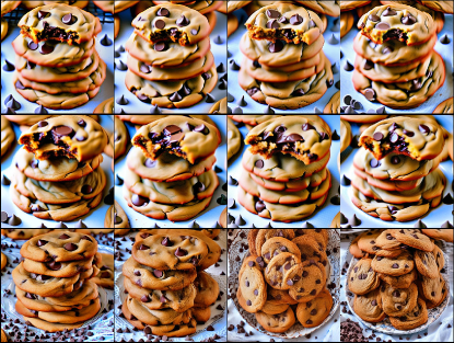
Figure 5: Generated samples using the prompt "A plate piled high with chocolate chip cookies.". From the top to bottom: first two SVGD for different realizations, and third row is $\gamma=30$ with CFG = 7.5 and 500 steps using NFSD.

Furthermore, CSD focuses in consistent visual synthesis across multiple samples for editing tasks, such as visual editing of panorama images, videos, and 3D scenes, while our goal is different.

B.5 Particle guidance

In the context of sampling, a recent work termed Particle guidance [9] proposed a method to incorporate an interactive particle sampler based on diffusion. They proposed a guidance term that couples a set of particles to guide the backwards diffusion process towards different modes of the target distribution. Although they leverage a similar idea, the scope of our work is different. Here we focus on diffusion model in the context of distillation, and therefore, as a regularizer, which allows to deploy in constrained problems like inverse problems, or unconstrained cases like text-to-3D.

Appendix C Unconstrained generation

The algorithm associated to RSD is shown in Alg. 1, where the repulsion term is the pairwise kernel function.

Algorithm 1 RSD for unconstrained generation

A generator $g_{\boldsymbol{\phi}}({\mathbf{m}})$ and a set of initial particles $\{{\mathbf{z}}_{i,0}^{0}=g_{\boldsymbol{\phi}^{(i)}}(.)\}_{i=1}^{n}$ and a decoder ${\mathcal{D}}(.)$

for $l=1\;\text{to}\;L$ do

     Sample $t\sim{\mathcal{U}}[0,T]$, $\xi\sim{\mathcal{N}}(0,{\mathbf{I}})$ and ${\mathbf{m}}$

     ${\mathbf{z}}_{i,0}^{\ell}=g_{\boldsymbol{\phi}^{(i)}}({\mathbf{m}})$

     ${\mathbf{z}}_{i,t}^{\ell}=\alpha_{t}{\mathbf{z}}_{i,0}^{\ell}+\sigma_{t}\boldsymbol{\epsilon}$

     ${\mathcal{L}}_{z}=\left[\lambda_{t}\;\mathrm{sg}\left[\nabla_{\mathbf{z}_{i,t}^{(\ell)}}\log p\left(\mathbf{z}_{i,t}^{(\ell)}\right)-\nabla_{\mathbf{z}_{i,t}^{\ell}}\log q_{\tau}\left(\mathbf{z}^{\ell}_{i,t}\right)\right]-\nabla_{{\mathbf{z}}_{t}^{(i)}}\gamma\sigma_{t}\log\sum_{j=1}^{N}k\left({\mathbf{z}}_{t}^{(i)},{\mathbf{z}}_{t}^{(j)}\right)\right]{\mathbf{z}}_{i,0}^{\ell}$

     for $i=1,\cdots,n$ do

         ${\mathbf{z}}_{i,0}^{\ell}=\mathrm{OptimizerStep}_{{\mathbf{z}}_{i,0}^{\ell}}({\mathcal{L}}_{z})$

     end for

end for

return $\{{\mathbf{x}}_{i,0}^{L}={\mathcal{D}}({\mathbf{z}}_{i,0}^{L})\}_{i=1}^{n}$

C.1 Implementation details

Details of experiment in Section

Here we describe the details of the experiments on 2D images with ProlificDreamer in the main text. We optimize 500 optimization steps as we found that was enough for our goal, which is studying the trade-off between quality and diversity; in Appendix C.2, we show experiments with more steps. We follow their setup, and we train a U-Net from scratch to estimate the variational score. We consider ADAM optimizer and set the learning rate of particle images is 0.03 and the learning rate of U-Net is 0.0001. We consider only 4 particles as it is enough to promote diversity (in particular when considering DINO as feature extractor). The images and parameters are initializad at random. We run all the experiments in a single NVIDIA A100 GPU of 80GB. The running time for ProlificDreamer for 2D generation with 500 iterations and 4 particles is 8 minutes when running in a Nvidia A100 GPU, while for the case of ProlificDreamer with repulsion using DINO is 12 minutes approx.

Regarding the similarity metric, we consider the cosine similarity in the range of DINO defined as follow

$$\text{Sim}({\mathbf{x}}_{1},\cdots,{\mathbf{x}}_{N})=\frac{1}{n(n-1)}\sum_{i\neq j}\frac{g_{\mathrm{DINO}}\left(\mathbf{x}_{i}\right)^{T}g_{\mathrm{DINO}}\left(\mathbf{x}_{j}\right)}{\left\|g_{\mathrm{DINO}}\left(\mathbf{x}_{i}\right)\right\|_{2}\left\|g_{\mathrm{DINO}}\left(\mathbf{x}_{j}\right)\right\|_{2}},$$ (37)

Base on this metric, we define diversity as

$$\text{Div}({\mathbf{x}}_{1},\cdots,{\mathbf{x}}_{N})=1-\text{Sim}({\mathbf{x}}_{1},\cdots,{\mathbf{x}}_{N}).$$ (38)

C.2 Ablation

C.2.1 Number of steps

In this subsection we consider different number of steps in the generation of unconstrained samples using ProlificDreamer. We consider 1000 steps instead of 500, with the same random strategy. The results for a subset of the images is shown in Table 2. Qualitative examples are shown in Figs 6. Our method enhances diversity when increasing the steps in the optimization; this is important for text-to-3D, where in general the amount of steps are higher (10k to 25k depending on the method).

Table 2: Results for the unconstrained case when considering 1000 steps in the optimization. We use ProlificDreamer.

	$\gamma=0$	$\gamma=20$	$\gamma=40$
Diversity	0.174	0.218	0.281
Aesthetic	5.382	5.303	5.273

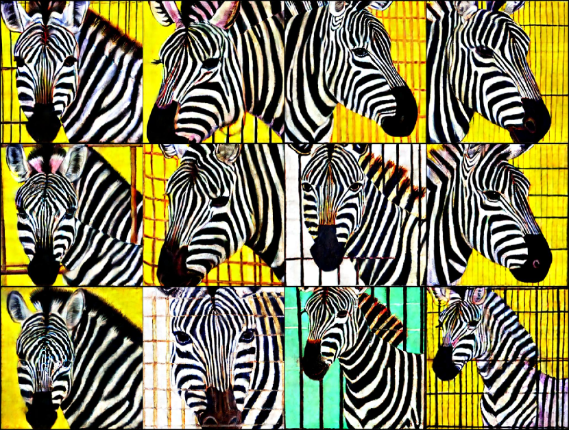
(a)

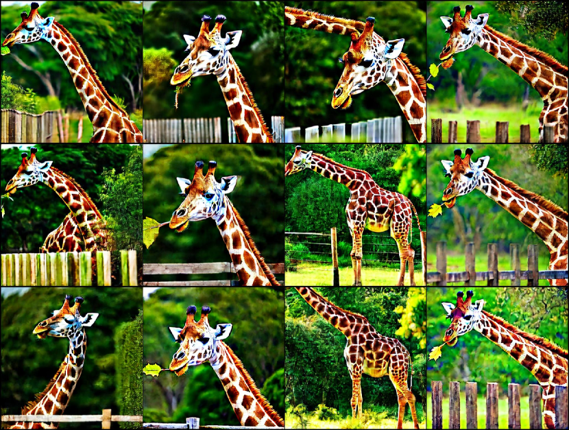
(b)

Figure 6: Generated samples using the prompt a) "the painting is of a zebra in a cage.", b) "a giraffe leaning it’s long neck over the fence to eat leaves off a bush." From the top to bottom: $\gamma=\{0,20,40\}$ with CFG = 7.5 and 1000 steps.

C.2.2 Number of particles

In this subsection we consider different number of steps in the generation of unconstrained samples using ProlificDreamer. We consider 1000 steps and 8 particles, with the same random strategy. The quantitative results for a subset of 10 images are shown in Table 3. This experiment shows that increasing the number of particles increase diversity as expected. However, this comes at the price of increasing the computational burden.

Table 3: Results for the unconstrained case when considering a batch of 8 particles in the optimization and 1000 steps. We use ProlificDreamer.

	$\gamma=0$	$\gamma=10$	$\gamma=20$
Diversity	0.183	0.209	0.232
Aesthetic	5.339	5.27	5.252

C.2.3 Guidance scale

One way of promoting diversity is by decreasing the guidance scale. Our proposed enhance regimes with low-CFG in terms of diversity without a big impact in the CLIP score. The results for a subset of 36 images with CFG = 4 under the same setting of the experimet in Section 6.1.2 is shown in Table 4. For a fair comparison, we also show the case of CFG = 7.5 for the same subset of images in Table 5. These two examples show that the repulsion enhances diversity for every case of CFG without compromising the text-alignment and quality of the generated images.

Table 4: Results for the unconstrained case when considering CFG = 4 (all the other hyperparemeters are the same as described in Appendix C.1. We use ProlificDreamer.

	$\gamma=0$	$\gamma=10$
Diversity	0.312	0.370
Aesthetic	5.240	5.257
CLIP	0.344	0.340

Table 5: Results for the unconstrained case when considering CFG = 7.5 (all the other hyperparemeters are the same as described in Appendix C.1. We use ProlificDreamer.

	$\gamma=0$	$\gamma=10$
Diversity	0.725	0.695
Aesthetic	5.216	5.194
CLIP	0.345	0.345

C.2.4 Using different domains/distances for the repulsion force

We compare the RBF when considering different domains, namely Euclidean, DINO and LPIPS.

RBF in the Euclidean domain.

We compare between DINO and RBF for a repulsion with $\gamma=10$, and the same setting than Section 6.1.2. We select a subset of 30 images. The quantitative results are shown in Table 6 and in Figs. 7 we show two qualitative examples.

Table 6: Comparison between RBF with distances with Euclidean distance vs DINO

	$\gamma=0$	$\gamma=10(\mathrm{Euclidean})$	$\gamma=10(\mathrm{DINO})$
Diversity	0.282	0.283	0.314
Aesthetic	5.178	5.179	5.164
CLIP	0.341	0.341	0.341

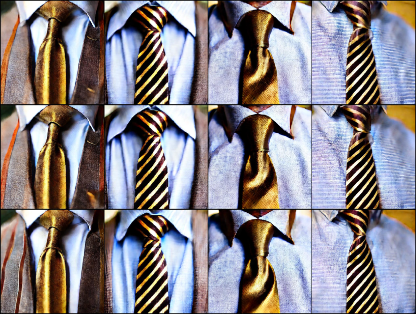
(a)

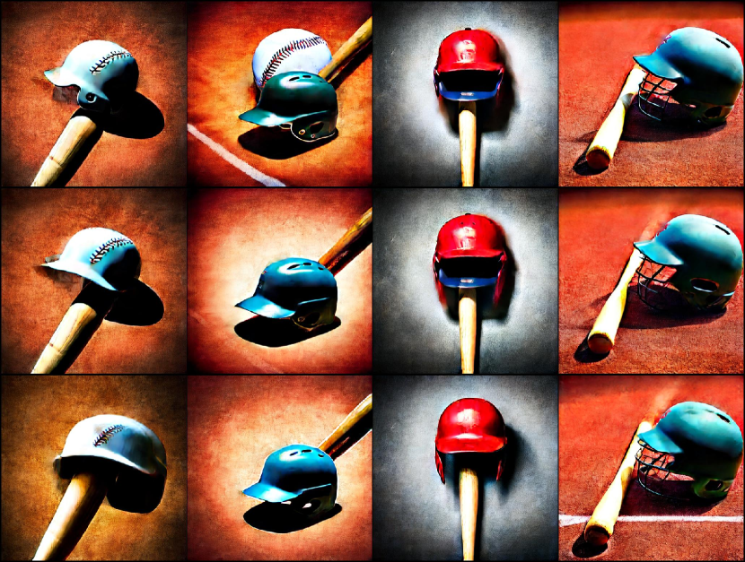
(b)

Figure 7: Comparison between RBF with Euclidean distance and DINO. We generate samples using the prompt a) "a gold tie is tied under a brown dress shirt with stripes..", b) "a baseball bat with a batting helmet upsidedown.". From the top to bottom: $\gamma=\{0,10(\mathrm{Euclidean}),10(\mathrm{DINO})\}$ with CFG = 7.5 and 500 steps.

RBF using LPIPS.

We also tried LPIPS as metric in RBF. However, we observe that when combined with ProlificDreamer, the generated images have some artifacts or are not well aligned with the text prompt; two exampes are shown in Figs. 8.

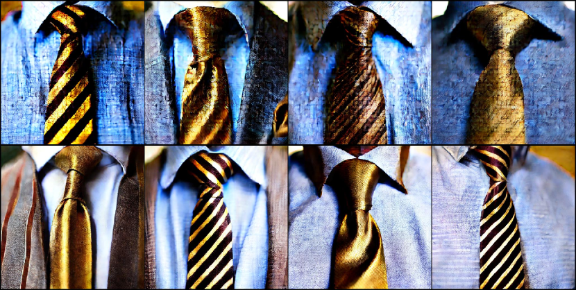
(a)

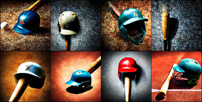
(b)

Figure 8: Comparison between RBF with Euclidean distance and DINO. We generate samples using the prompt a) "a gold tie is tied under a brown dress shirt with stripes..", b) "a baseball bat with a batting helmet upsidedown.". From the top to bottom: $\gamma=\{10(\mathrm{LPIPS}),10(\mathrm{DINO})\}$ with CFG = 7.5 and 500 steps.

C.3 Additional experiments for unconstrained case

C.3.1 Toy example with a Bimodal Gaussian distribution

We consider here a toy example to showcases how the $\gamma$ parameter (the amount of repulsion) dictates the trade-off between diversity and quality. We consider a mixture of two Gaussians of parameters ${\mathcal{N}}_{1}([1,0]^{\top},0.005{\mathbf{I}})$ and ${\mathcal{N}}_{2}([-1,0]^{\top},0.005{\mathbf{I}})$, and we consider two settings:

1. Two independent Gaussians with $\sigma\rightarrow 0$ where we fit the mean parameters

2. Two dependent Gaussians with $\sigma\rightarrow 0$ where we fit the mean parameters and coupled via an Euclidean RBF kernel.

For each setting, we compute 200 realizations with the same seed. In Fig. 9(a) we show how many realizations sufffers from mode-collapse ($\gamma=0$ corresponds to the first setting), while in Figs. 9(b) and 9(c) we show a realization for $\gamma=1$ and $\gamma=2000$, where we observe that the "quality" of the estimation for this high value is poorer compared to $\gamma=1$.

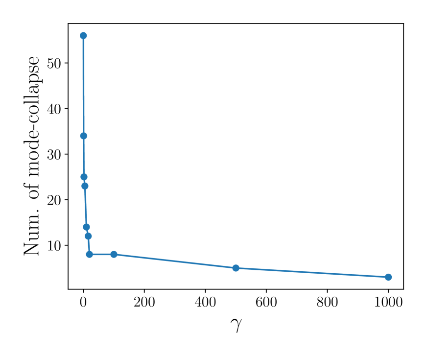
(a)

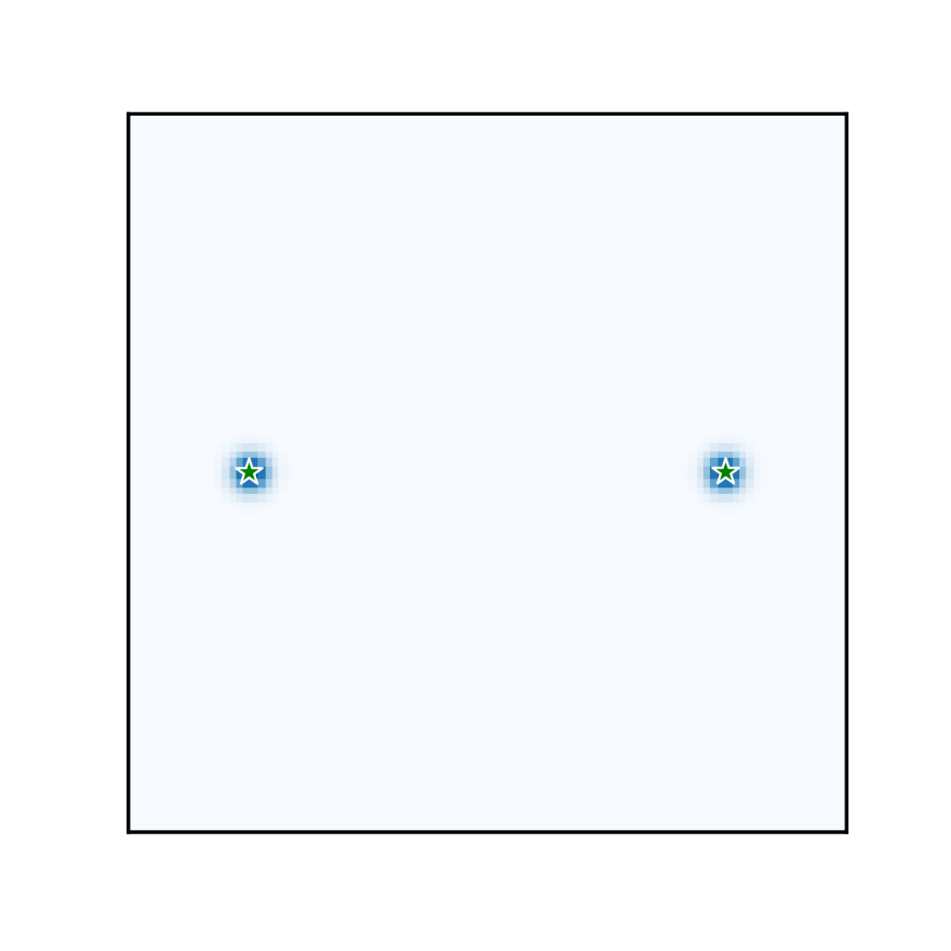
(b)

(c)

Figure 9: a) Number of realizations that has a particle collapse to the same mode as a function of the amount of repulsion that we consider. Estimation when considering b) $\gamma=1$, c) $\gamma=2000$.

C.3.2 Additional results for trade-off plot

In Fig. 11 we show the trade off plot with the corresponding error bars. Notice that the dispersion decreases consistently when increasing the repulsion weight. Furthermore, notice that score distillation achieves a better Aesthetic score due to its oversaturation, but the FID is worst. And more important, the diversity is very low due to its high CFG (100).

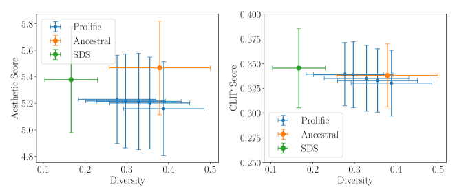
Figure 10:

Figure 11: Trade-off plot with the corresponding error bars.

C.3.3 Additional results for ProlificDreamer with repulsion

We show in Figs. 12 and  13. some examples that we used to compute Fig. 3.

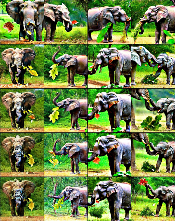
Figure 12: RSD with ProlificDreamer as base method. Generated samples using the prompt "An elephant placing some leaves in its mouth with its trunk.". From the top to the lowest: $\gamma=\{0,10,20,30,40\}$ with CFG = 7.5.

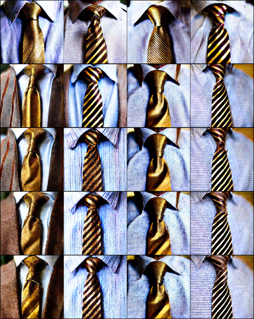
(a)

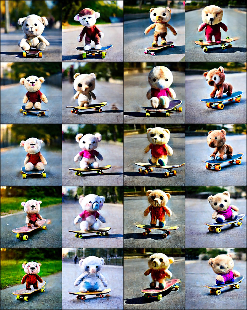
(b)

Figure 13: RSD with ProlificDreamer as base method. Generated samples using the prompt a) "a gold tie is tied under a brown dress shirt with stripes." (left column), b) "A stuffed animal that is frowning is on a skateboard."(right column). From top to bottom $\gamma=\{0,10,20,30,40\}$ with CFG = 7.5.

C.3.4 Additional results for NFSD with repulsion

To showcase the generality of our method, we show in Figs. 14,  15 and 16 qualitative results using NFSD [28]. Notice that the backgrounds for the images generated with repulsion have different details while the cases without repulsion are similar.

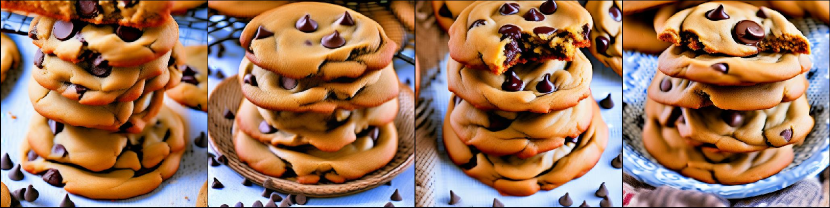
(a) NSFD

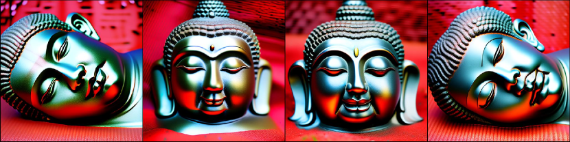
(b) NFSD

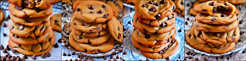
(c) NFSD with repulsion

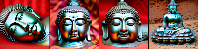
(d) NFSD with repulsion

Figure 14: Similar to Fig. 2, we aim to show that adding repulsion yields a more diverse set of images while keeping a good visual quality using NFSD. a, c) Generated samples using the prompt "A plate piled high with chocolate chip cookies". a) NFSD with a pairwise similarity of 0.81 , c) NFSD with repulsion and a pairwise similarity of 0.77. b, d) Generated samples using the prompt "A metal lying Buddah". b) NFSD with a pairwise similarity of 0.79 , d) NFSD with repulsion and a pairwise similarity of 0.72.

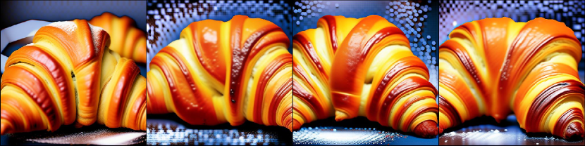
(a) NSFD

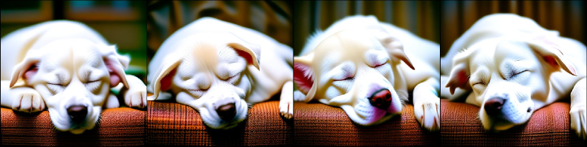
(b) NSFD

(c) NFSD with repulsion ($\gamma=40$)

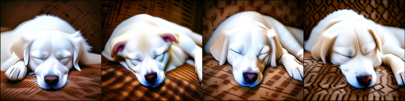
(d) NFSD with repulsion ($\gamma=30$)

Figure 15: RSD with NFSD as base method. a, c) Generated samples using the prompt "A delicious croissant". a) NFSD with a pairwise similarity of 0.87 , c) NFSD with repulsion and a pairwise similarity of 0.85. b, d) Generated samples using the prompt "A white dog sleeping". a) NFSD with a pairwise similarity of 0.92 , b) NFSD with repulsion and a pairwise similarity of 0.85.

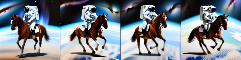
(a) NSFD

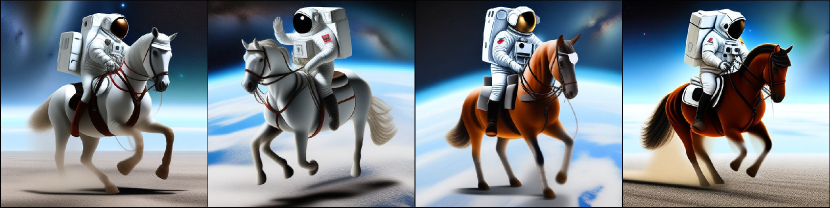
(b) NFSD with repulsion ($\gamma=30$)

Figure 16: RSD with NFSD as base method. a, b) Generated samples using the prompt "An astronaut riding a horse". a) NFSD with a pairwise similarity of 0.92 , b) NFSD with repulsion and a pairwise similarity of 0.87.

C.3.5 Additional results for text-to-3D generation

We show in this Section more experiments in text-to-3D generation and more details about the implementation.

Implementation details.

For the NeRF architecture we use an MLP, and we use the same configuration from the setting in Threestudio. For the diffusion model, we use DeepFloyd-IF-XL-v1.0 with a guidance scale of 20. For the repulsion, we use a repulsion weight of $\gamma=200\sigma_{t}$. We use one Nvidia A100 of 80GB, and we consider a batch of 20 particles. For the RBF, we use DINO.

Results.

We show in Fig. 17. Notice that our method the cases without repulsion have the same shape and each part of the bulldozer has the same color: the blades in the front are yellow, the roofs are yellow and black, and the only difference is in the wheels. On the other hand, the cases with repulsion have different colors for the front blade (yellow and black), different color for the roof, and the front design is different as well.

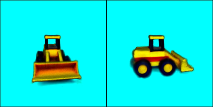
(a) Without repulsion - Seed 1

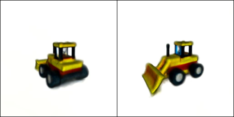
(b) Without repulsion - Seed 35

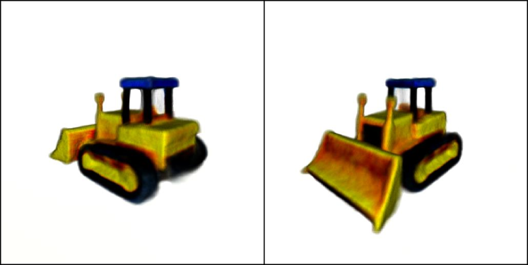
(c) With repulsion - Seed 1

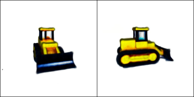
(d) With repulsion - Seed 35

Figure 17: Text-to-3D generation using DreamFusion with the prompt "a bulldozer made out of toy bricks", and considering a batch of 20 samples (particles) a, b) without repulsion with seed 1 and seed 35, c, d) with repulsion with seed 1 and 34 respectively. For each case, we show two different views.

Appendix D Constrained generation: inverse problems

D.1 Diffusion for inverse problems

Diffusion models are powerful generative model. Therefore, they have been used as deep generative prior to solve inverse problems. Given a pre-trained diffusion models, this involves running the backward process using a guidance (likelihood) term, that incorporates the measurement information. Formally, we can sample from the posterior $p({\mathbf{x}}_{0}|{\mathbf{y}})$ by running (39)

$$d{\mathbf{x}}_{t}=-\frac{1}{2}\beta(t){\mathbf{z}}_{t}\text{d}t-\beta(t)\left[\nabla_{{\mathbf{x}}_{t}}\log p({\mathbf{x}}_{t})+\nabla_{{\mathbf{x}}_{t}}\log p({\mathbf{y}}|{\mathbf{x}}_{t})\right]+\sqrt{\beta(t)}\text{d}{\mathbf{W}}_{t}.$$ (39)

Early studies used Langevin dynamics for linear problems [26, 29, 35, 66], while others used DDPM [30, 7, 6, 21]. However, approximating the guidance term remains a challenge. Previous works addressed this with a Gaussian approximation of $p({\mathbf{x}}_{0}|{\mathbf{x}}_{t})$ around the MMSE estimator via Tweedie’s formula, increasing computational burden [5, 52, 26, 53]. These methods crudely approximate the posterior score, especially for non-small noise levels. One of the most effective methods is DPS [5], which assumes:

$$p\left({\mathbf{y}}|{\mathbf{x}}_{t}\right)\approx p\left({\mathbf{y}}|{\hat{\mathbf{x}}}_{0}:=\mathbb{E}\left[{\mathbf{x}}_{0}|{\mathbf{x}}_{t}\right]\right)=\mathcal{N}\left({\mathbf{y}}|f(\mathbb{E}\left[{\mathbf{x}}_{0}|{\mathbf{x}}_{t}\right]),\sigma_{t}^{2}{\mathbf{I}}\right).$$

Essentially, DPS approximates the likelihood with a unimodal Gaussian distribution center around the MMSE estimator $\mathbb{E}\left[{\mathbf{x}}_{0}|{\mathbf{x}}_{t}\right]$. Under this approximation, the term $p\left({\mathbf{y}}|{\mathbf{x}}_{t}\right)$ boils down to the gradient of a multivariate Gaussian. Although it achieves impressive results, the unimodal approximation is far from optimal. Furthermore, its adaption to use latent diffusion model is not straightforward as explained in [46]. Recent works [46, 50, 31, 8] extended this by sampling from the latent space of diffusion models but still face limitations due to the intractable model likelihood.

D.2 Implemetation details of RSD

For all the cases, unless we stated in other way, we consider $1000$ steps (the full denoising trajectory). We consider ADAM optimizer to train the parameters, and set the momentum pair $(0.9,0.99)$. We initialize both variables ${\mathbf{x}}$ and ${\mathbf{z}}$ at random, and we consider a descending schedule from $t=T$ to $t=1$. We generate a batch of 4 particles per noisy measurement. Regarding the pre-trained model, we consider Stable diffusion v1.5 (which was the one used in PSLD). Moreover, other latent diffusion models such as LDM pre-trained on FFHQ can be used. We consider $\omega=0$ in (24). Regarding the timesteps, we consider descending order following the scheme from [41], where the descending case achieved the best performance.

Random inpainting.

In this case we use $\lambda=0.001$, $\frac{1}{\rho^{2}}=0.009$, $l_{r_{x}}=0.4$ and $l_{r_{z}}=0.8$.

Inpainting Half face.

In this case we use $\lambda=0.01$, $\frac{1}{\rho^{2}}=0.075$, $l_{r_{x}}=0.4$ and $l_{r_{z}}=0.8$.

Free masks from [48].

For the images in Appendix D.4.3, we consider the same hypeparameters than inpainting half face.

Algorithm for solving inverse problems with augmented variational distribution.

In Alg. 2 we show the algorithm for solving inverse problems with repulsion and score-matching regularization; the operation sg denotes stop gradient. We run all the experiments in a single NVIDIA A100 GPU of 80GB. The running time for our solver depends on the number of steps, but for the full trajectory it takes around 13-15 minutes to generate 4 particles, and using the repulsion term.

Algorithm 2 RSD for solving inverse problems

A target distribution $p({\mathbf{x}}_{0},{\mathbf{z}}_{0}|{\mathbf{y}})$ and a set of initial particles $\{{\mathbf{x}}_{i}^{0},{\mathbf{z}}_{i,0}^{0}\}_{i=1}^{n}$

for $l=1\;\text{to}\;L$ do

     Sample $t\sim{\mathcal{U}}[0,T]$ and $\xi\sim{\mathcal{N}}(0,{\mathbf{I}})$

     ${\mathbf{z}}_{i,t}^{\ell}=\alpha_{t}{\mathbf{z}}_{i,0}^{\ell}+\sigma_{t}\boldsymbol{\epsilon}$

     ${\mathcal{L}}_{z}=\sum_{i=1}^{n}\|{\mathbf{x}}_{i}^{\ell}-{\mathcal{D}}({\mathbf{z}}_{i,0}^{\ell})\|^{2}+\left(\lambda_{t}\text{sg}\left[\epsilon({\mathbf{z}}_{i,t}^{\ell},t)-\boldsymbol{\epsilon}\right]\right)^{\top}{\mathbf{z}}_{i,0}^{\ell}$

                                        $-\text{sg}\left[\nabla_{{\mathbf{z}}_{t}^{(i)}}\gamma\sigma_{t}\log\sum_{j=1}^{N}k\left({\mathbf{z}}_{t}^{(i)},{\mathbf{z}}_{t}^{(j)}\right)\right]^{\top}{\mathbf{z}}_{i,0}^{\ell}$

     for $i=1,\cdots,n$ do

         ${\mathbf{z}}_{i,0}^{\ell}=\mathrm{OptimizerStep}_{{\mathbf{z}}_{i,0}^{\ell}}({\mathcal{L}}_{z})$

     end for

     ${\mathcal{L}}_{x}=\sum_{i=1}^{n}\|{\mathbf{y}}-{\mathbf{f}}({\mathbf{x}}_{i}^{l})\|^{2}+\|{\mathbf{x}}_{i}^{l}-{\mathcal{D}}({\mathbf{z}}_{i,0}^{l})\|^{2}$

     for $i=1,\cdots,n$ do

         ${\mathbf{x}}_{i,0}^{\ell}=\mathrm{OptimizerStep}_{{\mathbf{x}}_{i,0}^{\ell}}({\mathcal{L}}_{x})$

     end for

end for

return $\{{\mathbf{x}}_{i,0}^{L}={\mathcal{D}}({\mathbf{z}}_{i,0}^{L})\}_{i=1}^{n}$

D.3 Comparison between augmented vs non-augmented variational sampler

We compare in Fig. 18 the augmented vs non-augmented variational sampler; the non-augmented corresponds to the optimization of ${\mathbf{z}}$ only. Notice that our method with augmentation achieves a better result compared to the non-augmented case in terms of blurriness. We validate this with numerical results below for random and box inpainting.

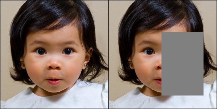
(a)

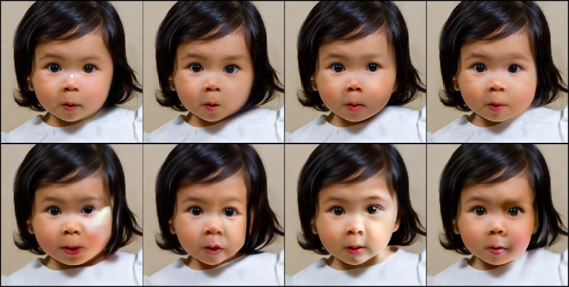
(b)

Figure 18: Comparison between RSD (top row of Fig. b), which is Augmented RED-diff, and RED-diff in latent space, which is non-Augmented (last row of Fig. b).

D.4 Additional results

D.4.1 Inpainting with half-face box

We additionally compare against SOTA diffusion samplers that operates in the pixel domain. We consider DPS [5] and RED-diff [41], and we use the pre-trained model from [5] on FFHQ. The results are shown in Table 7. Given that image-based diffusion solvers generate images at $256\times 256$, we follow the strategy from [46] and downsample the results generated by our sampler. In Figs. 19, 20 and 21 we show some of the results.

Table 7: Box inpainting (half face) with $\sigma_{v}=0.001$. The best method for each metric and experiment is bolded.

Method	PSNR [dB] $\uparrow$	LPIPS $\downarrow$	FID $\downarrow$
PSLD	20.66	0.16	57.7
RSD ($\gamma=0$)	24.98	0.079	29.18
RED-Diff	23.1	0.067	29.79
DPS	21.35	0.166	112.9

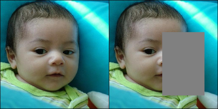
(a)

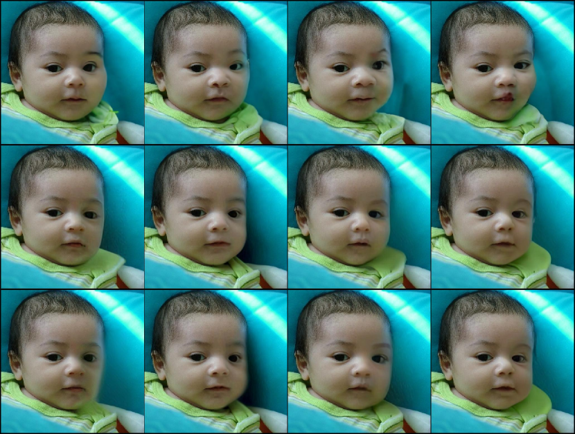
(b)

Figure 19: Results for inpainting half face using (from top to bottom): PSLD, RSD ($\gamma=0$) and RSD ($\gamma=50$).

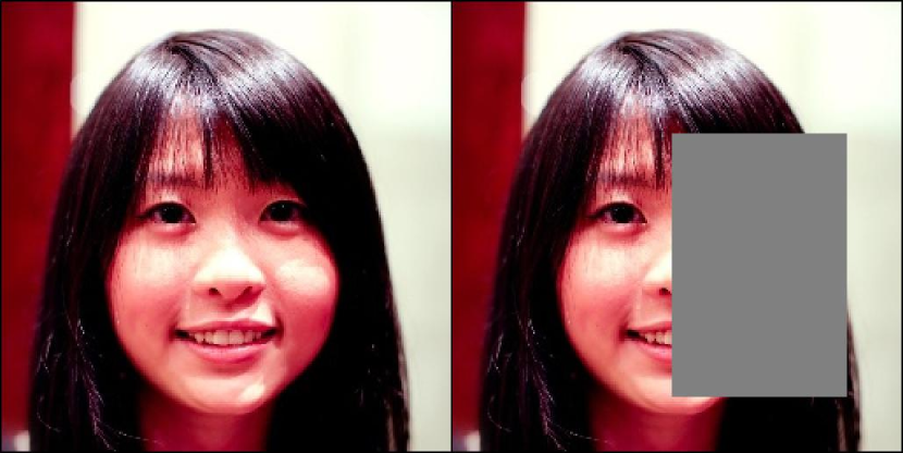
(a)

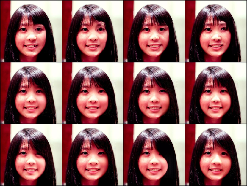
(b)

Figure 20: Results for inpainting half face using (from top to bottom): PSLD, RSD ($\gamma=0$) and RSD ($\gamma=50$).

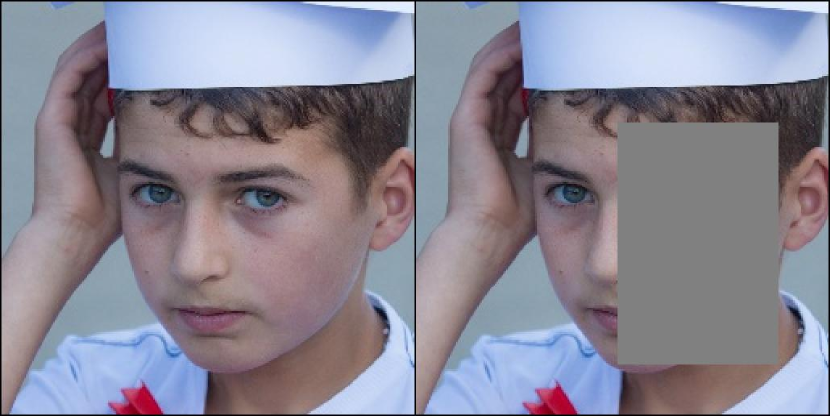
(a)

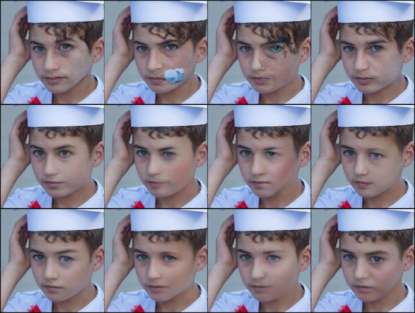
(b)

Figure 21: Results for inpainting half face using (from top to bottom): PSLD, RSD ($\gamma=0$) and RSD ($\gamma=50$).

D.4.2 Inpainting with random mask ($p=0.8$)

We consider random inpainting where we drop $80\%$ of the pixels. The numerical results are shown in Table 8, and visual examples are shown in Fig. 22.

Table 8: Quantitative results on noisy images ($\sigma_{v}=0.001$) for random (80%) mask. In bold is the best method for each metric and experiment.

Method	PSNR [dB] $\uparrow$	LPIPS $\downarrow$	FID $\downarrow$
PSLD	28.53	0.212	65.14
RSD ($\gamma=0$)	30.56	0.145	41.11

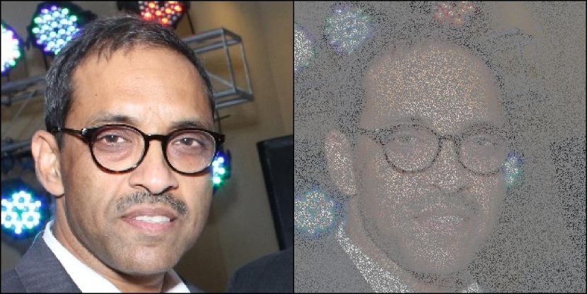
(a)

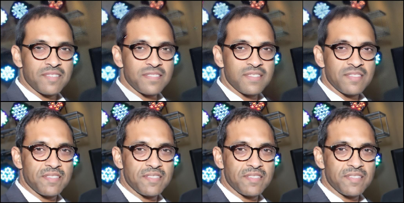
(b)

Figure 22: Results for random inpainting for PSLD (top) and RSD ($\gamma=0$) (down). Notice that RSD generates a better reconstruction of the background.

D.4.3 Images beyond FFHQ

Here we show some examples of reconstruction using out-of-distribution images; we use samples from ImageNet [47]. In Fig. 23 we show an example from ImageNet, where we compare RSD with RED-diff using FFHQ. Clearly, the performance of RSD is better than RED-diff. This is expected given that the diffusion model of RED-diff is with FFHQ. However, this demonstrates that using more powerful diffusion model as prior enables to deploy our model for different type of images.

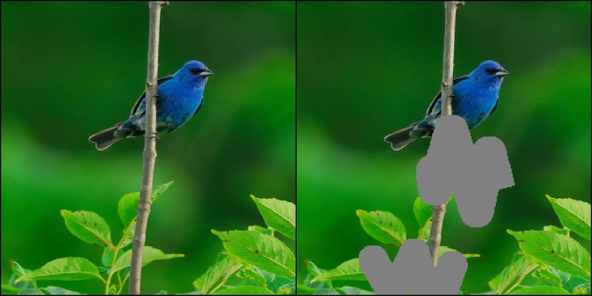
(a)

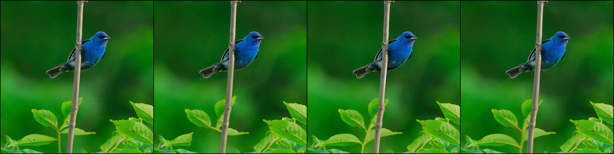
(b)

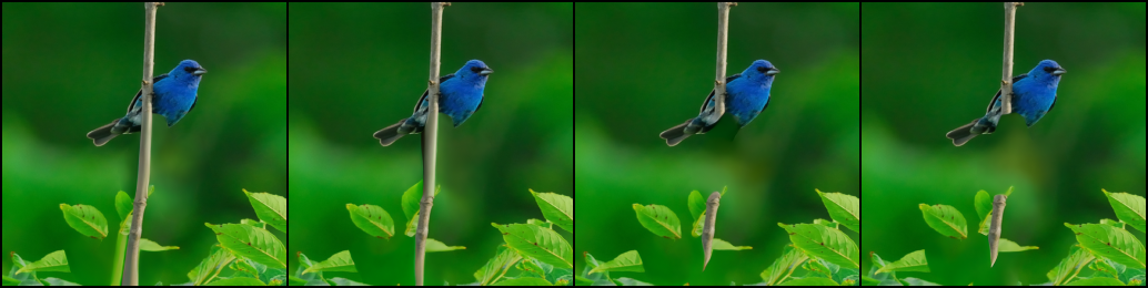
(c)

Figure 23: Results of the reconstruction using RSD (b) and RED-diff (c) with FFHQ with ImageNet example.

References

- Armandpour et al. [2023] Mohammadreza Armandpour, Huangjie Zheng, Ali Sadeghian, Amir Sadeghian, and Mingyuan Zhou. Re-imagine the negative prompt algorithm: Transform 2D diffusion into 3D, alleviate janus problem and beyond. arXiv preprint arXiv:2304.04968, 2023.
- Ba et al. [2021] Jimmy Ba, Murat A Erdogdu, Marzyeh Ghassemi, Shengyang Sun, Taiji Suzuki, Denny Wu, and Tianzong Zhang. Understanding the variance collapse of SVGD in high dimensions. In Intl. Conf. Learn. Repr. (ICLR), 2021.
- Caron et al. [2021] Mathilde Caron, Hugo Touvron, Ishan Misra, Hervé Jégou, Julien Mairal, Piotr Bojanowski, and Armand Joulin. Emerging properties in self-supervised vision transformers. In Proceedings of the IEEE/CVF Int. Conf. Comput. Vis. (ICCV), pages 9650–9660, 2021.
- Chen et al. [2023] Yifan Chen, Daniel Zhengyu Huang, Jiaoyang Huang, Sebastian Reich, and Andrew M Stuart. Gradient flows for sampling: mean-field models, Gaussian approximations and affine invariance. arXiv preprint arXiv:2302.11024, 2023.
- Chung et al. [2022a] Hyungjin Chung, Jeongsol Kim, Michael Thompson Mccann, Marc Louis Klasky, and Jong Chul Ye. Diffusion posterior sampling for general noisy inverse problems. In Intl. Conf. Learn. Repr. (ICLR), 2022a.
- Chung et al. [2022b] Hyungjin Chung, Byeongsu Sim, Dohoon Ryu, and Jong Chul Ye. Improving diffusion models for inverse problems using manifold constraints. Advances in Neural Inf. Process. Syst. (NIPS), 35:25683–25696, 2022b.
- Chung et al. [2022c] Hyungjin Chung, Byeongsu Sim, and Jong Chul Ye. Come-closer-diffuse-faster: Accelerating conditional diffusion models for inverse problems through stochastic contraction. In Proceedings of the IEEE/CVF Int. Conf. Comput. Vis. Pattern Recogn. (CVPR), pages 12413–12422, 2022c.
- Chung et al. [2024] Hyungjin Chung, Jong Chul Ye, Peyman Milanfar, and Mauricio Delbracio. Prompt-tuning latent diffusion models for inverse problems. Intl. Conf. on Machine Learning (ICML), 2024.
- Corso et al. [2024] Gabriele Corso, Yilun Xu, Valentin De Bortoli, Regina Barzilay, and Tommi Jaakkola. Particle guidance: non-IID diverse sampling with diffusion models. Intl. Conf. Learn. Repr. (ICLR), 2024.
- D’Angelo and Fortuin [2021a] Francesco D’Angelo and Vincent Fortuin. Annealed Stein variational gradient descent. arXiv preprint arXiv:2101.09815, 2021a.
- D’Angelo and Fortuin [2021b] Francesco D’Angelo and Vincent Fortuin. Repulsive deep ensembles are Bayesian. Advances in Neural Inf. Process. Syst. (NIPS), 34:3451–3465, 2021b.
- Dockhorn et al. [2021] Tim Dockhorn, Arash Vahdat, and Karsten Kreis. Score-based generative modeling with critically-damped Langevin diffusion. In Intl. Conf. Learn. Repr. (ICLR), 2021.
- Duncan et al. [2023] Andrew Duncan, Nikolas Nüsken, and Lukasz Szpruch. On the geometry of Stein variational gradient descent. J. Mach. Learn. Res., 24(56):1–39, 2023.
- Faye et al. [2024] Elhadji C Faye, Mame Diarra Fall, and Nicolas Dobigeon. Regularization by denoising: Bayesian model and Langevin-within-split Gibbs sampling. arXiv preprint arXiv:2402.12292, 2024.
- Geman and Yang [1995] Donald Geman and Chengda Yang. Nonlinear image recovery with half-quadratic regularization. IEEE transactions on Image Processing, 4(7):932–946, 1995.
- Graikos et al. [2022] Alexandros Graikos, Nikolay Malkin, Nebojsa Jojic, and Dimitris Samaras. Diffusion models as plug-and-play priors. Advances in Neural Inf. Process. Syst. (NIPS), 35:14715–14728, 2022.
- Guo et al. [2023] Yuan-Chen Guo, Ying-Tian Liu, Ruizhi Shao, Christian Laforte, Vikram Voleti, Guan Luo, Chia-Hao Chen, Zi-Xin Zou, Chen Wang, Yan-Pei Cao, and Song-Hai Zhang. threestudio: A unified framework for 3d content generation. https://github.com/threestudio-project/threestudio, 2023.
- Hessel et al. [2021] Jack Hessel, Ari Holtzman, Maxwell Forbes, Ronan Le Bras, and Yejin Choi. CLIPScore: A reference-free evaluation metric for image captioning. In Proceedings of Conferenc on Empirical Methods in Natural Language Processing. Association for Computational Linguistics, 2021.
- Ho and Salimans [2021] Jonathan Ho and Tim Salimans. Classifier-free diffusion guidance. In NeurIPS 2021 Workshop on Deep Generative Models and Downstream Applications, 2021.
- Ho et al. [2020] Jonathan Ho, Ajay Jain, and Pieter Abbeel. Denoising diffusion probabilistic models. Advances in Neural Inf. Process. Syst. (NIPS), 33:6840–6851, 2020.
- Ho et al. [2022] Jonathan Ho, Tim Salimans, Alexey Gritsenko, William Chan, Mohammad Norouzi, and David J Fleet. Video diffusion models. Advances in Neural Inf. Process. Syst. (NIPS), 35:8633–8646, 2022.
- Hong et al. [2024] Susung Hong, Donghoon Ahn, and Seungryong Kim. Debiasing scores and prompts of 2D diffusion for view-consistent text-to-3D generation. Advances in Neural Inf. Process. Syst. (NIPS), 36, 2024.
- Hu et al. [2021] Edward J Hu, Phillip Wallis, Zeyuan Allen-Zhu, Yuanzhi Li, Shean Wang, Lu Wang, Weizhu Chen, et al. LoRA: Low-rank adaptation of large language models. In Intl. Conf. Learn. Repr. (ICLR), 2021.
- Jain et al. [2022] Ajay Jain, Ben Mildenhall, Jonathan T Barron, Pieter Abbeel, and Ben Poole. Zero-shot text-guided object generation with dream fields. In Proceedings of the IEEE/CVF Int. Conf. Comput. Vis. Pattern Recogn. (CVPR), pages 867–876, 2022.
- Jordan et al. [1998] Richard Jordan, David Kinderlehrer, and Felix Otto. The variational formulation of the Fokker–Planck equation. SIAM J. Math. Anal., 29(1):1–17, 1998.
- Kadkhodaie and Simoncelli [2021] Zahra Kadkhodaie and Eero Simoncelli. Stochastic solutions for linear inverse problems using the prior implicit in a denoiser. Advances in Neural Inf. Process. Syst. (NIPS), 34:13242–13254, 2021.
- Karras et al. [2019] Tero Karras, Samuli Laine, and Timo Aila. A style-based generator architecture for generative adversarial networks. In Proceedings of the IEEE/CVF Int. Conf. Comput. Vis. Pattern Recogn. (CVPR), pages 4401–4410, 2019.
- Katzir et al. [2024] Oren Katzir, Or Patashnik, Daniel Cohen-Or, and Dani Lischinski. Noise-free score distillation. In Intl. Conf. Learn. Repr. (ICLR), 2024.
- Kawar et al. [2021] Bahjat Kawar, Gregory Vaksman, and Michael Elad. SNIPS: Solving noisy inverse problems stochastically. Advances in Neural Inf. Process. Syst. (NIPS), 34:21757–21769, 2021.
- Kawar et al. [2022] Bahjat Kawar, Michael Elad, Stefano Ermon, and Jiaming Song. Denoising diffusion restoration models. Advances in Neural Inf. Process. Syst. (NIPS), 35:23593–23606, 2022.
- Kim et al. [2024] Jeongsol Kim, Geon Yeong Park, and Jong Chul Ye. Dreamsampler: Unifying diffusion sampling and score distillation for image manipulation. arXiv preprint arXiv:2403.11415, 2024.
- Kim et al. [2023] Subin Kim, Kyungmin Lee, June Suk Choi, Jongheon Jeong, Kihyuk Sohn, and Jinwoo Shin. Collaborative score distillation for consistent visual editing. In Advances in Neural Inf. Process. Syst. (NIPS), volume 36, pages 73232–73257, 2023.
- Kong et al. [2020] Zhifeng Kong, Wei Ping, Jiaji Huang, Kexin Zhao, and Bryan Catanzaro. DiffWave: A versatile diffusion model for audio synthesis. In Intl. Conf. Learn. Repr. (ICLR), 2020.
- Lambert et al. [2022] Marc Lambert, Sinho Chewi, Francis Bach, Silvère Bonnabel, and Philippe Rigollet. Variational inference via Wasserstein gradient flows. Advances in Neural Inf. Process. Syst. (NIPS), 35:14434–14447, 2022.
- Laumont et al. [2022] Rémi Laumont, Valentin De Bortoli, Andrés Almansa, Julie Delon, Alain Durmus, and Marcelo Pereyra. Bayesian imaging using plug & play priors: when Langevin meets Tweedie. SIAM J. Imag. Sciences, 15(2):701–737, 2022.
- Lin et al. [2014] Tsung-Yi Lin, Michael Maire, Serge Belongie, James Hays, Pietro Perona, Deva Ramanan, Piotr Dollár, and C Lawrence Zitnick. Microsoft coco: Common objects in context. In European Conf. Comp. Vision (ECCV), pages 740–755. Springer, 2014.
- Liu [2017] Qiang Liu. Stein variational gradient descent as gradient flow. Advances in Neural Inf. Process. Syst. (NIPS), 30, 2017.
- Liu and Wang [2016] Qiang Liu and Dilin Wang. Stein variational gradient descent: A general purpose Bayesian inference algorithm. Advances in Neural Inf. Process. Syst. (NIPS), 29, 2016.
- Liu et al. [2022] Xiaodong Liu, Li Wei, Yuntao Huang, and Lu Yuan. Diffusion models for text-to-3d generation. arXiv preprint arXiv:2210.10723, 2022.
- Luo et al. [2024] Weijian Luo, Tianyang Hu, Shifeng Zhang, Jiacheng Sun, Zhenguo Li, and Zhihua Zhang. Diff-instruct: A universal approach for transferring knowledge from pre-trained diffusion models. Advances in Neural Inf. Process. Syst. (NIPS), 36, 2024.
- Mardani et al. [2024] Morteza Mardani, Jiaming Song, Jan Kautz, and Arash Vahdat. A variational perspective on solving inverse problems with diffusion models. Intl. Conf. Learn. Repr. (ICLR), 2024.
- Poole et al. [2022] Ben Poole, Ajay Jain, Jonathan T Barron, and Ben Mildenhall. Dreamfusion: Text-to-3D using 2D diffusion. In Intl. Conf. Learn. Repr. (ICLR), 2022.
- Poole et al. [2023] Ben Poole, Ajay Jain, Jonathan T Barron, and Ben Mildenhall. Dreamfusion: Text-to-3d using 2d diffusion priors. arXiv preprint arXiv:2304.09367, 2023.
- Romano et al. [2017] Yaniv Romano, Michael Elad, and Peyman Milanfar. The little engine that could: Regularization by denoising (RED). SIAM J. Imag. Sciences, 10(4):1804–1844, 2017.
- Rombach et al. [2021] Robin Rombach, Andreas Blattmann, Dominik Lorenz, Patrick Esser, and Björn Ommer. High-resolution image synthesis with latent diffusion models. 2022 ieee. In Proceedings of the IEEE/CVF Int. Conf. Comput. Vis. Pattern Recogn. (CVPR), pages 10674–10685, 2021.
- Rout et al. [2024] Litu Rout, Negin Raoof, Giannis Daras, Constantine Caramanis, Alex Dimakis, and Sanjay Shakkottai. Solving linear inverse problems provably via posterior sampling with latent diffusion models. Advances in Neural Inf. Process. Syst. (NIPS), 36, 2024.
- Russakovsky et al. [2015] Olga Russakovsky, Jia Deng, Hao Su, Jonathan Krause, Sanjeev Satheesh, Sean Ma, Zhiheng Huang, Andrej Karpathy, Aditya Khosla, Michael Bernstein, et al. Imagenet large scale visual recognition challenge. Int. J. Comp. Vision, 115:211–252, 2015.
- Saharia et al. [2022] Chitwan Saharia, William Chan, Huiwen Chang, Chris Lee, Jonathan Ho, Tim Salimans, David Fleet, and Mohammad Norouzi. Palette: Image-to-image diffusion models. In ACM SIGGRAPH 2022 conference proceedings, pages 1–10, 2022.
- Sohl-Dickstein et al. [2015] Jascha Sohl-Dickstein, Eric Weiss, Niru Maheswaranathan, and Surya Ganguli. Deep unsupervised learning using nonequilibrium thermodynamics. In Intl. Conf. on Machine Learning (ICML), pages 2256–2265. PMLR, 2015.
- Song et al. [2024] Bowen Song, Soo Min Kwon, Zecheng Zhang, Xinyu Hu, Qing Qu, and Liyue Shen. Solving inverse problems with latent diffusion models via hard data consistency. Intl. Conf. Learn. Repr. (ICLR), 2024.
- Song et al. [2020] Jiaming Song, Chenlin Meng, and Stefano Ermon. Denoising diffusion implicit models. In Intl. Conf. Learn. Repr. (ICLR), 2020.
- Song et al. [2022] Jiaming Song, Arash Vahdat, Morteza Mardani, and Jan Kautz. Pseudoinverse-guided diffusion models for inverse problems. In Intl. Conf. Learn. Repr. (ICLR), 2022.
- Song et al. [2023] Jiaming Song, Qinsheng Zhang, Hongxu Yin, Morteza Mardani, Ming-Yu Liu, Jan Kautz, Yongxin Chen, and Arash Vahdat. Loss-guided diffusion models for plug-and-play controllable generation. In Intl. Conf. on Machine Learning (ICML), pages 32483–32498. PMLR, 2023.
- Song et al. [2021a] Yang Song, Conor Durkan, Iain Murray, and Stefano Ermon. Maximum likelihood training of score-based diffusion models. Advances in Neural Inf. Process. Syst. (NIPS), 34:1415–1428, 2021a.
- Song et al. [2021b] Yang Song, Jascha Sohl-Dickstein, Diederik P Kingma, Abhishek Kumar, Stefano Ermon, and Ben Poole. Score-based generative modeling through stochastic differential equations. In Intl. Conf. Learn. Repr. (ICLR), 2021b.
- Team [2022] LAION-AI Team. Laion-aesthetics predictor v2. https://github.com/christophschuhmann/improved-aesthetic-predictor,2022, 2022.
- Vahdat et al. [2021] Arash Vahdat, Karsten Kreis, and Jan Kautz. Score-based generative modeling in latent space. Advances in Neural Inf. Process. Syst. (NIPS), 34:11287–11302, 2021.
- Van Dyk and Meng [2001] David A Van Dyk and Xiao-Li Meng. The art of data augmentation. J. Comp. Graph. Stat., 10(1):1–50, 2001.
- Venkatakrishnan et al. [2013] Singanallur V Venkatakrishnan, Charles A Bouman, and Brendt Wohlberg. Plug-and-play priors for model based reconstruction. In IEEE Global Conf. Signal and Info. Process. (GlobalSIP), pages 945–948. IEEE, 2013.
- Vincent [2011] Pascal Vincent. A connection between score matching and denoising autoencoders. Neural computation, 23(7):1661–1674, 2011.
- Vono et al. [2020] Maxime Vono, Nicolas Dobigeon, and Pierre Chainais. Asymptotically exact data augmentation: Models, properties, and algorithms. J. Comp. Graph. Stat., 30(2):335–348, 2020.
- Wang et al. [2023] Peihao Wang, Dejia Xu, Zhiwen Fan, Dilin Wang, Sreyas Mohan, Forrest Iandola, Rakesh Ranjan, Yilei Li, Qiang Liu, Zhangyang Wang, et al. Taming mode collapse in score distillation for text-to-3D generation. arXiv preprint arXiv:2401.00909, 2023.
- Wang et al. [2024] Zhengyi Wang, Cheng Lu, Yikai Wang, Fan Bao, Chongxuan Li, Hang Su, and Jun Zhu. Prolificdreamer: High-fidelity and diverse text-to-3D generation with variational score distillation. Advances in Neural Inf. Process. Syst. (NIPS), 36, 2024.
- Zhu et al. [2023] Yuanzhi Zhu, Kai Zhang, Jingyun Liang, Jiezhang Cao, Bihan Wen, Radu Timofte, and Luc Van Gool. Denoising diffusion models for plug-and-play image restoration. In Proceedings of the IEEE/CVF Int. Conf. Comput. Vis. Pattern Recogn. (CVPR), pages 1219–1229, 2023.
- Zilberstein et al. [2022] Nicolas Zilberstein, Chris Dick, Rahman Doost-Mohammady, Ashutosh Sabharwal, and Santiago Segarra. Annealed Langevin dynamics for massive MIMO detection. IEEE Trans. Wireless Commun., 2022.
- Zilberstein et al. [2024] Nicolas Zilberstein, Ashutosh Sabharwal, and Santiago Segarra. Solving linear inverse problems using higher-order annealed Langevin diffusion. IEEE Trans. Signal Process., 2024.