Towards Communication-Efficient Peer-to-Peer Networks

Abstract

We focus on designing Peer-to-Peer (P2P) networks that enable efficient communication. Over the last two decades, there has been substantial algorithmic research on distributed protocols for building P2P networks with various desirable properties such as high expansion, low diameter, and robustness to a large number of deletions. A key underlying theme in all of these works is to distributively build a random graph topology that guarantees the above properties. Moreover, the random connectivity topology is widely deployed in many P2P systems today, including those that implement blockchains and cryptocurrencies. However, a major drawback of using a random graph topology for a P2P network is that the random topology does not respect the underlying (Internet) communication topology. This creates a large propagation delay, which is a major communication bottleneck in modern P2P networks.

In this paper, we work towards designing P2P networks that are communication-efficient (having small propagation delay) with provable guarantees. Our main contribution is an efficient, decentralized protocol, Close-Weaver, that transforms a random graph topology embedded in an underlying Euclidean space into a topology that also respects the underlying metric. We then present efficient point-to-point routing and broadcast protocols that achieve essentially optimal performance with respect to the underlying space.

1 Introduction

There has been a long line of algorithmic research on building Peer-to-Peer (P2P) networks (also called overlay networks) with desirable properties such as connectivity, low diameter, high expansion, and robustness to adversarial deletions [35, 28, 17, 9, 10, 22, 5]. A key underlying theme in these works is a distributed protocol to build a random graph that guarantees these desirable properties. The high-level idea is for a node to connect to a small, but random, subset of nodes. In fact, this random connectivity mechanism is used in real-world P2P networks. For example, in the Bitcoin P2P network, each node connects to 8 neighbors chosen in a random fashion [30]. It is well-known that a random (bounded-degree) graph is an expander with high probability. An expander graph on $n$ nodes has high expansion and conductance, low diameter (logarithmic in the network size) and robustness to adversarial deletions — even deleting $\epsilon n$ nodes (for a sufficiently small constant $\epsilon$) leaves a giant component of $\Theta\mathchoice{\left(n\right)}{(n)}{(n)}{(n)}$ size which is also an expander [20, 7].

Unfortunately, a major drawback of using a random graph as a P2P network is that the connections are made to random nodes and do not respect the underlying (Internet) communication topology. This causes a large propagation latency or delay. Indeed, this is a crucial problem in the Bitcoin P2P network, which has delays as high as 79 seconds on average [11, 30]. A main cause for the delay is that the P2P (overlay) network induced by random connectivity can be highly sub-optimal, since it ignores the underlying Internet communication topology (which depends on geographical distance, among other factors). The main problem we address in this paper is to show how one can efficiently modify a given random graph topology to build P2P networks that also have small propagation latency, in addition to other properties such as low (hop) diameter and high expansion, with provable guarantees.

Towards this goal, following prior work (see e.g. [30, 12]), we model a P2P network as a random graph embedded in an underlying Euclidean space. This model is a reasonable approximation to a random connectivity topology on nodes distributed on the Internet (details in Section 1.1).

The main contributions of this paper are: (1) a theoretical framework to rigorously quantify performance of P2P communication protocols; (2) Close-Weaver, an efficient decentralized protocol that converts the random graph topology into a topology that also respects the underlying embedding; (3) efficient point-to-point routing and broadcast algorithms in the modified topology that achieve essentially optimal performance. We note that broadcasting is a key application used in P2P networks that implement blockchain and cryptocurrencies in which a block must be quickly broadcast to all (or most) nodes in the network.

1.1 Motivation, Model, and Definitions

Motivation. We consider a random graph network that is used in several prior P2P network construction protocols (e.g. [35, 28, 9, 5]). As mentioned earlier, real-world P2P networks, such as Bitcoin, also seek to achieve a random graph topology (which are expanders with high probability [32, 20]). Indeed, random graphs have been used extensively to model P2P networks (see e.g. [28, 35, 17, 9, 29]).

Before we formally state the model that is based on prior works [30, 12, 21], we explain the motivation behind it; we refer to [30] for more details and give a brief discussion here. Many of today’s P2P (overlay) networks employ the random connectivity algorithm; in fact, this is widely deployed in many cryptocurrency systems. In this algorithm, nodes maintain a small number of connections to other nodes chosen in a random fashion. In such a topology, for any two nodes $u$ and $v$, any path (including the shortest path) would likely go through nodes that are not located close to the shortest geographical route (i.e., the geodesic) connecting $u$ and $v$. Such paths that do not respect the underlying geographical placement of nodes often lead to higher propagation delay. Indeed, it can be shown that a random topology yields paths with propagation delays much higher than those of paths on topologies that respect the underlying geography [30].

To model the underlying propagation costs, several prior works (see e.g., the Vivaldi system [12]) have empirically shown that nodes on the Internet can be embedded on a low-dimensional metric space (e.g., $\mathbb{R}^{5}$) such that the distance between any two nodes accurately captures the communication delay between them. In fact, the Vivaldi system demonstrates that even embedding the nodes in a 2-dimensional metric space (e.g., $\mathbb{R}^{2}$) and using the corresponding distances captures the communication delay quite well. In contrast, the paths on a random graph topology are highly sub-optimal, since they are unlikely to follow the optimal path on the embedded metric space.

The work of Mao et al. [30] illustrates the above disparity using the following example motivated by the above discussion. Consider a network embedded in the unit square $[0,1]\times[0,1]$ (see Figure 1).

Figure 1: Nodes in a random graph topology embedded in the unit square. Notice that the straight-line distance from $u$ to $v$ is much shorter than sum of the distances in a shortest path between the two nodes.

The set of nodes (points) $V$ is drawn uniformly at random within the square. The Euclidean distance, $\mathchoice{\left\lVert u-v\right\rVert}{\lVert u-v\rVert}{\lVert u-v\rVert}{\lVert u-v\rVert}_{2}$, between any two nodes $u,v\in V$ represents the delay or latency of sending a message from $u$ to $v$ (or vice-versa). We construct a random graph on $V$ by connecting each node in the unit-square randomly to a small constant number of other nodes. Figure 1 shows the shortest path on this topology between two nodes, say $u$ (bottom left corner) to $v$ (top right corner). Since the random graph does not respect the underlying geometry, the propagation cost between $u$ and $v$ — defined as the sum of the Euclidean distances of the edges in the shortest path — is significantly greater than the point-to-point (geodesic) distance ($\mathchoice{\left\lVert u-v\right\rVert}{\lVert u-v\rVert}{\lVert u-v\rVert}{\lVert u-v\rVert}_{2}$) between them. We formally show this in Theorem 1.4.

By comparison, consider a random geometric graph on $V$, where the uniformly distributed nodes are connected as follows: any two nodes $u$ and $v$ are connected by an edge if they are within a distance $\rho$ of each other [38, 33]. This model, called the $G(n,\rho)$ random geometric graph model, has connections which respect the underlying geometry. In this graph, we can show that the shortest path between any two nodes $u$ and $v$ is much closer to the geodesic shortest path (the straight line path) between $u$ and $v$ [33, 14].

We note that, while the work of Mao et al. [30] showcases the disparity between a random graph and a random geometric graph (as discussed above) it does not give any theoretical results on how to convert a random graph topology into a random geometric graph topology. On the other hand, it gives heuristics to transform a P2P graph constructed on real-world data to a graph that has smaller propagation delays. The heuristics are based on rewiring edges to favor edges between nodes that have smaller round-trip delays. It presents experimental simulations to show that these heuristics do well in practice. However, they do not formally analyze their algorithm and do not give any theoretical guarantees.

Network Model.  Motivated by the above discussion, and following prior works [30, 12, 21], we model a P2P network $G$ as follows. We assume $G$ to be a $d$-regular expander (where $d$ is a constant). Note that our results will also apply if $G$ has a random connectivity topology modeled by a $d$-regular (or bounded degree) random graph or a $G(n,p)$ random graph (with $p=\Theta\mathchoice{\left(\log n/n\right)}{(\log n/n)}{(\log n/n)}{(\log n/n)}$). We note that such random graphs are expanders with high probability (see Definition 1.12) [26]. Our model is quite general in the sense that we only assume that the topology is an expander; no other special properties are assumed. (Indeed, expanders have been used extensively to model P2P networks [28, 35, 17, 9, 29, 6, 5].) Furthermore, we assume that the nodes of $G$ correspond to points that are distributed uniformly at random in a unit square $[0,1]\times[0,1]$. Although, the assumption of nodes being uniformly distributed is strong, based on our experiments on the Bitcoin P2P network, this appears to be a reasonable first approximation. Considering more general distribution models is a good direction for future work (cf. Section 1.5).

We assume each node $u$ knows its ID and, while node $u$ need not know its coordinates, it is able to determine its distance (which captures propagation delay) to any node $v$ given only the ID of $v$. In particular, we assume for convenience that a node can determine the Euclidean and the Manhattan distances (i.e., $L_{2}$ and $L_{\infty}$ norms respectively) between itself and another node if it knows the ID of that node.

An important assumption is that nodes initially have only local knowledge, i.e., they have knowledge of only themselves and their neighbors in $G$. In particular, they do not have any knowledge of the global topology or of the IDs of other nodes (except those of their neighbors) in the network. We assume that nodes have knowledge of the network size $n$ (or a good estimate of it).

We assume a synchronous network where computation and communication proceeds in a sequence of discrete rounds. Communication is via message passing on the edges of $G$. Note that $G$ is a P2P (overlay) network in the sense that a node $u$ can communicate (directly) with another node $v$ if $u$ knows the ID of $v$. This is a typical assumption in the context of P2P and overlay networks, where a node can establish communication with another node if it knows the other node’s IP address, and has been used in several prior works (see e.g. [5, 4, 22, 36, 18]). Note that $u$ can know the ID of $v$ either directly, because $u$ and $v$ are neighbours in $G$, or indirectly, through received messages. In the latter case, this is equivalent to adding a “virtual” edge between $u$ and $v$. Since we desire efficient protocols, we require each node to send and receive messages of size at most $\operatorname{polylog}{(n)}$ bits in a round. In fact, a node will also communicate with only $\operatorname{polylog}{(n)}$ other nodes in a round. Additionally, the number of bits sent per edge per round is $O\mathchoice{\left(\operatorname{polylog}{(n)}\right)}{(\operatorname{polylog}{(n)})}{(\operatorname{polylog}{(n)})}{(\operatorname{polylog}{(n)})}$.

1.2 Preliminaries

We need the following concepts before we formally state the problem that we address and our contributions.

Embedded Graph. We define an embedded graph as follows.

Definition 1.1.

Let $G=(V,E)$ be any graph and consider a random embedding of the nodes $V$ into the unit square, i.e., a uniform and independent assignment of coordinates in $[0,1]\times[0,1]$ to each node in $V$. This graph, together with this embedding, is called an embedded graph, and we induce weights on the edge set $E$, with the weight of an edge $(u,v)$ equal to the Euclidean distance between the coordinates assigned to $u$ and $v$, respectively.

Routing Cost. We next define propagation cost to capture the cost of routing along a path in an embedded graph.

Definition 1.2.

Let $G$ be an embedded graph. For any path $P=(v_{1},v_{2},\dots,v_{k-1},v_{k})$ the propagation cost, also called the routing propagation cost, of the path $P$ is the weight of the path $P$ given by $d_{G}(P)=\sum_{i=1}^{k-1}d(v_{i},v_{i+1})$, i.e., the sum of the weights (the Euclidean distances) of edges along the path. The value $k$, denoted by $\operatorname{hopcount}_{G}(P)$, is the hop count (or hop length) of the path $P$. The minimum propagation cost between the nodes $u$ and $v$ is the weight of the shortest path between $u$ and $v$ in the embedded graph.

Note that the propagation cost between two nodes is lower bounded by the Euclidean distance between them. Given two nodes, we would like to route using a path of small propagation cost, i.e., a path whose propagation cost is close to the Euclidean distance between the two nodes. In particular, we would like the ratio between the two to be small. (We would also like the hop count to be small.)

The following theorem shows that, in a $d$-regular random graph $G$ embedded in the unit square, the ratio of the propagation cost of the shortest path between two nodes $u$ and $v$ in $G$ to the Euclidean distance between those nodes can be as high as $\Omega(\sqrt{n})$ on expectation. Thus a P2P topology that is modeled by a random graph topology has a high propagation cost for some node pairs.

We first prove the following lemma.

Lemma.

Let $G$ be an embedded (connected) $d$-regular graph, for any constant $d\geq 2$. There exist a pair of nodes, $u$ and $v$, such that $d(u,v)=O\mathchoice{\left(1/\sqrt{n}\right)}{(1/\sqrt{n})}{(1/\sqrt{n})}{(1/\sqrt{n})}$ and all shortest paths $P$ between $u$ and $v$ have $\Omega\mathchoice{\left(\log{n}\right)}{(\log{n})}{(\log{n})}{(\log{n})}$ hops and $\mathbb{E}\mathchoice{\left[d(P)\right]}{[d(P)]}{[d(P)]}{[d(P)]}$, the expected value of the sum of the Euclidean distances of the edges along this path, is $\Omega\mathchoice{\left(1\right)}{(1)}{(1)}{(1)}$.

Proof 1.3.

Fix a node $u$. Since $G$ is $d$-regular, we can show that there exists a set $S$ of $\epsilon n$ nodes (for some fixed constant $\epsilon>0$ that depends on $d$) that is at least $c\log{n}$ hops away from $u$ (for a suitably small constant $c>0$). Fix this set $S$ of $\epsilon n$ nodes. Consider the square of side-length $1/\sqrt{n}$ (and thus area $1/n$) centered at $u$ — with probability

$$\binom{\epsilon n}{1}\frac{1}{n}\left(1-\frac{1}{n}\right)^{\epsilon n-1}=\epsilon\left(1-\frac{1}{n}\right)^{\epsilon n-1}\approx\epsilon\exp\left(-\epsilon\frac{n-1}{n}\right)=\Theta\mathchoice{\left(1\right)}{(1)}{(1)}{(1)}$$

exactly one of nodes in the set $S$ (call it $v$) falls within this square. Clearly, $d(u,v)=O\mathchoice{\left(1/\sqrt{n}\right)}{(1/\sqrt{n})}{(1/\sqrt{n})}{(1/\sqrt{n})}$.

Now, consider any path from $u$ to $v$; any such path has to go through a neighbor of $u$. The probability that a single node has distance at least $\delta$ from $u$ is simply the area of the circle of radius $\delta$ centered at $u$, which is $\pi\delta^{2}$. Hence for a fixed constant $\delta>0$, with probability $\left(1-\pi\delta^{2}\right)^{d}=\Theta(1)$ all $d$ neighbors of $u$ in $G$ (note that these $d$ neighbors are disjoint from the nodes in set $S$ that are at least $c\log{n}$ hops away) will have distance at least $\delta$ from $u$. Thus, for constant $\delta$, at least one edge on every path from $u$ to $v$ will have expected length $\Omega\mathchoice{\left(1\right)}{(1)}{(1)}{(1)}$ and, by the triangle inequality, every such path has distance at least $\Omega\mathchoice{\left(1\right)}{(1)}{(1)}{(1)}$.

Theorem 1.4.

Let $G$ be a $d$-regular random graph embedded in the unit square. Then, there exists a pair of nodes $u$ and $v$ in $G$ such that $d_{G}(P)/d(u,v)$, the ratio of the propagation cost of the shortest path $P$ between $u$ and $v$ to the Euclidean distance between them is $\Omega\mathchoice{\left(\sqrt{n}\right)}{(\sqrt{n})}{(\sqrt{n})}{(\sqrt{n})}$ on expectation.

Proof 1.5.

Take $u$ and $v$ as in Lemma Lemma. Note that $d(u,v)=O\mathchoice{\left(1/\sqrt{n}\right)}{(1/\sqrt{n})}{(1/\sqrt{n})}{(1/\sqrt{n})}$ and that any shortest path between $u$ and $v$ has expected total distance $\Omega\mathchoice{\left(1\right)}{(1)}{(1)}{(1)}$. Thus, the ratio of the propagation cost of the shortest path between them to the Euclidean distance between them is simply

$$\frac{\Omega\mathchoice{\left(1\right)}{(1)}{(1)}{(1)}}{O\mathchoice{\left(1/\sqrt{n}\right)}{(1/\sqrt{n})}{(1/\sqrt{n})}{(1/\sqrt{n})}}=\Omega\mathchoice{\left(\sqrt{n}\right)}{(\sqrt{n})}{(\sqrt{n})}{(\sqrt{n})}.$$

We use propagation cost to measure the performance of a routing algorithm in $G$. The goal is to construct a graph topology so that one can find paths of small propagation costs between every pair of nodes. Moreover, we want a routing algorithm that routes along paths of small propagation cost while also keeping the hop length small.

Broadcast Performance Measures. Next, we quantify the performance of a broadcasting algorithm.

Definition 1.6.

Consider a broadcast algorithm $\mathcal{A}$ that broadcasts a single message from a given source to all other nodes in some connected embedded graph $G$. The broadcast propagation cost of algorithm $\mathcal{A}$ on graph $G$ is defined as the the sum of the Euclidean distance of the edges used by $\mathcal{A}$ to broadcast the message.

Notice that the broadcast propagation cost roughly captures the efficiency of a broadcast algorithm. We note that the best possible broadcast propagation cost for a graph is broadcasting by using only the edges of the minimum spanning tree (MST) on $G$. In particular, this yields the following lower bound for a graph whose nodes are embedded uniformly at random in the unit square. The proof follows from a bound on the weight of a Euclidean MST on a set of points distributed uniformly in a unit square [2].

Theorem 1.7.

[follows from [2]] The broadcast propagation cost of any algorithm $\mathcal{A}$ on an embedded graph $G$ whose nodes are distributed uniformly in a unit square is $\Omega\mathchoice{\left(\sqrt{n}\right)}{(\sqrt{n})}{(\sqrt{n})}{(\sqrt{n})}$ with high probability.

On the other hand, we show that the broadcast propagation cost of the standard flooding algorithm [37] on a random graph embedded in a unit square is high compared to the above lower bound.

Theorem 1.8.

Let $G$ be a $d$-regular random graph embedded in the unit square. The standard flooding algorithm on $G$ has $\Theta\mathchoice{\left(n\right)}{(n)}{(n)}{(n)}$ expected broadcast propagation cost.

Proof 1.9.

The message will be sent across every edge at least once. Thus, $\sum_{(u,v)\in E}w(u,v)$ is a lower bound on the propagation cost, where $w(u,v)$ is the Euclidean distance between two nodes $u$ and $v$. We use the principle of deferred decisions to bound the expected value of the weight (Euclidean distance) of an edge. Fix an edge $e=(u,v)$ in the graph and consider its expected length. Since $u$ and $v$ are chosen uniformly at random in the unit square, it is easy to show that the $\mathbb{E}\mathchoice{\left[w(u,v)\right]}{[w(u,v)]}{[w(u,v)]}{[w(u,v)]}=\Theta(1)$. Hence by linearity of expectation

$$\sum_{(u,v)\in E}w(u,v)=\frac{dn}{2}\cdot\Theta\mathchoice{\left(1\right)}{(1)}{(1)}{(1)}=\Theta\mathchoice{\left(n\right)}{(n)}{(n)}{(n)}.$$

We also use other metrics to measure the quality of a broadcast algorithm $\mathcal{A}$. The broadcast completion cost and broadcast completion time measure, respectively, the propagation cost and the number of hops needed to reach any other node $v$ from a given source $u$.

Definition 1.10.

Consider a broadcast algorithm $\mathcal{A}$ that broadcasts a single message from some source node $z$ to all other nodes in some connected graph $G(V,E)$. The broadcast completion cost of $\mathcal{A}$ on $G$ is the maximum value of the minimum propagation cost between the source node $s$ and any node $u$ considering paths taken by the message in $\mathcal{A}$, taken over all nodes $u\in V$ and all possible source nodes $s\in V$. More precisely, let $\operatorname{Prop}_{\mathcal{A}}(s,u)$ be the minimum propagation cost for a message sent from the node $s$ to reach node $u$ using broadcast algorithm $\mathcal{A}$ and define $\operatorname{Prop}_{\mathcal{A}}(s)=\max_{u\in V}\operatorname{Prop}_{\mathcal{A}}(s,u)$. Then, broadcast completion cost is $\max_{s\in V}\operatorname{Prop}_{\mathcal{A}}(s)$. The broadcast completion time of $\mathcal{A}$ on $G$ is simply the number of rounds before the message from the source node reaches all nodes.

Conductance and Expanders. We recall the notions of conductance of a graph and that of an expander graph.

Definition 1.11 (Conductance).

The conductance $\phi(G)$ of a graph $G=(V,E)$ is defined as: $\phi(G)=\min_{S\subseteq V}\frac{\mathchoice{\left\lvert E(S,\overline{S})\right\rvert}{\lvert E(S,\overline{S})\rvert}{\lvert E(S,\overline{S})\rvert}{\lvert E(S,\overline{S})\rvert}}{\min\mathchoice{\left\{\operatorname{Vol}{S},\operatorname{Vol}\overline{S}\right\}}{\{\operatorname{Vol}{S},\operatorname{Vol}\overline{S}\}}{\{\operatorname{Vol}{S},\operatorname{Vol}\overline{S}\}}{\{\operatorname{Vol}{S},\operatorname{Vol}\overline{S}\}}}$ where, for any set $S$, $E(S,\overline{S})$ denotes the set of all edges with one vertex in $S$ and one vertex in $\overline{S}=V-S$, and $\operatorname{Vol}(S)$, called the volume of $S$, is the sum of the degrees of all nodes in $S$.

Definition 1.12 (Expander Graph).

A family of graphs $G_{n}$ on $n$ nodes is an expander family if, for some constant $\alpha$ with $0<\alpha<1$, the conductance $\phi_{n}=\phi(G_{n})$ satisfies $\phi_{n}\geq\alpha$ for all $n\geq n_{0}$ for some $n_{0}\in\mathbb{N}$.

Random Geometric Graph.

Definition 1.13 (Random Geometric Graph).

A random geometric graph, $G(n,\rho)=(V,E)$, is a graph of $n$ points, independently and uniformly at random placed within $[0,1]\times[0,1]$ (the unit square). These points form the node set $V$, and for two nodes $u$ and $v$, $(u,v)\in E$ if and only if the distance $d(u,v)$ is at most $\rho$, for parameter $0<\rho=f(n)\leq 1$.

We note that the distance between points is the standard Euclidean distance. The $G(n,\rho)$ graph exhibits the threshold phenomenon for many properties, such as connectivity, coverage, presence of a giant component, etc. [38, 33]. For example, the threshold for connectivity is $\rho=\Theta\mathchoice{\left(\sqrt{\log n/n}\right)}{(\sqrt{\log n/n})}{(\sqrt{\log n/n})}{(\sqrt{\log n/n})}$, i.e., if the value of $\rho$ is $\Omega\mathchoice{\left(\sqrt{\log n/n}\right)}{(\sqrt{\log n/n})}{(\sqrt{\log n/n})}{(\sqrt{\log n/n})}$, the graph $G(n,\rho)$ is connected with high probability; on the other hand, if $\rho=o\mathchoice{\left(\sqrt{\log n/n}\right)}{(\sqrt{\log n/n})}{(\sqrt{\log n/n})}{(\sqrt{\log n/n})}$, then the graph is likely to be disconnected. It is also known [15] that the diameter of $G(n,\rho)$ (above the connectivity threshold) is $\tilde{\Theta}(1/\rho)$ with high probability.

1.3 Problems Addressed and Our Contributions

As shown in Theorems 1.4 and 1.8, routing (even via the shortest path) and the standard flooding broadcast protocol in an embedded random graph $G$ have a relatively large point-to-point routing propagation cost and broadcast propagation cost, respectively.

Given a P2P network modeled as a random graph $G$ embedded on a unit square, the goal is to design an efficient distributed protocol to transform $G$ into a network $G^{*}$ that admits efficient communication primitives for the fundamental tasks of routing and broadcast, in particular, those that have essentially optimal routing and broadcast propagation costs. Furthermore, we want to design optimal routing and broadcast protocols on $G^{*}$. (Broadcasting is a key application used in P2P networks that implement blockchain and cryptocurrencies in which a block must be quickly broadcast to all (or most) nodes in the network.)

Our contributions are as follows:

1. We develop a theoretical framework to model and analyze P2P network protocols, specifically point-to-point routing and broadcast (see Section 1.1).

2. We present an efficient distributed P2P topology construction protocol, Close-Weaver, that takes a P2P expander network $G$ and improves it into a topology $G^{*}$ that admits essentially optimal routing and broadcast primitives (see Section 2). Our protocol uses only local knowledge and is fast, using only $O(\operatorname{polylog}{n})$ rounds. Close-Weaver is based on random walks which makes it quite lightweight (small local computation overhead) and inherently decentralized and robust (no single point of action, no construction of tree structure, etc). It is also scalable in the sense that each node sends and receives only $O(\operatorname{polylog}{n})$ bits per round and communicates with only $O(\operatorname{polylog}{n})$ nodes at any round. We assume only that the given topology $G$ is an expander graph; in particular, $G$ can be random graph (modeling a random connectivity topology, see Section 1.1).

3. To show the efficiency of $G^{*}$, we develop a distributed routing protocol Greedy-Routing as well as broadcast protocols Geometric-Flooding and Compass-Cast that have essentially optimal routing and broadcast propagation costs, respectively (see Section 3).

1.4 Technical Overview

1.4.1 Close-Weaver protocol

The high-level idea behind Close-Weaver is as follows. Starting from an expander graph, the goal is to construct a topology that (i) contains a random geometric graph and (ii) contains a series of graphs such that each graph is an expander with edges that respect a maximum upper bound on Euclidean distance, for various distance values. This topology will then be used to design efficient communication protocols (Section 3). To construct a random geometric graph, nodes must discover other nodes that are close to them in the Euclidean space; in particular, each node $u$ needs to connect to all nodes within distance $\rho=\Theta(\sqrt{\log n/n})$ to form a connected random geometric graph (see Definition 1.13). The challenge is, in the given expander graph, nodes do not have knowledge of the IDs of other nodes (except their neighbors in the original graph) in the network. The protocol allows each node to find nodes that are progressively closer in distance to itself. From $G$, which is an expander in the unit square, we construct several expander graphs in squares of smaller side-length. The expander graph is constructed by each node connecting to a small number of random nodes in the appropriate square. This creates a random graph which we show to be an expander with high probability (Lemma 2.2). Connecting to random nodes is accomplished by performing lazy random walks which mix fast (i.e., reach the uniform stationary distribution) due to the expander graph property [20]. We show a key technical lemma (Lemma 2.2) that proves the expansion property of the expanders created by random walks by analyzing the conductance of the graph. By constructing expander graphs around each node in progressively smaller areas, the protocol finally is able to locate all nearby (within distance $\rho=\Theta(\sqrt{\log n/n})$) nodes with high probability. Then each node forms connections to these nodes, which guarantees that a random geometric graph is included as a subgraph. The final constructed graph $G^{*}$ includes all the edges that were created by the protocol, in addition to the edges in the original graph $G$. Thus, $G^{*}$ is an expander (with degree bounded by $O(\log^{2}n)$) and also includes a random geometric graph as a subgraph (among other edges added by nodes to random nodes at varying distances).

1.4.2 P2P Routing Protocol

We note that the original graph $G$ does not admit an efficient point-to-point routing protocol as it is a random graph and is not addressable. Note that even if one uses shortest path routing (assuming shortest paths have been constructed a priori), the propagation cost can be as high as $\Omega(\sqrt{n})$ (see Theorem 1.4).

We present a P2P routing protocol, called Greedy-Routing, with near-optimal propagation cost in $G^{*}$. The key benefit of our routing protocol is that it is fully-localized, i.e., a node $u$ needs only the ID of the destination node $v$ and the distances of its neighbors to $v$ to determine to which neighbor it should forward the message. In particular, we show that a simple greedy protocol that always forwards the message to a neighbor closest to the destination correctly and efficiently routes the message. Routing protocols that assume that each node knows its own position and that of its neighbors and that the position of the destination is known to the source are sometimes referred to as geometric routing and greedy approaches to such routing have been explored in the literature (e.g, [25], [24], [27] and the references therein). We show that Greedy-Routing takes $O\mathchoice{\left(\log n\right)}{(\log n)}{(\log n)}{(\log n)}$ hops to reach the destination and, more importantly, that the propagation cost is close to the optimal propagation cost needed to route between the two nodes. Our protocol carefully exploits the geometric structure of the constructed edges created in $G^{*}$ to show the desired guarantees.

1.4.3 P2P Broadcast Protocols

We see that any broadcast algorithm that runs on the type of input graphs we consider takes at least $\Omega(\sqrt{n})$ broadcast propagation cost with high probability (Theorem 1.7). However, if we ran a simple flooding algorithm on the original graph, we could only achieve a broadcast propagation cost of $\Theta(n)$ on expectation (see Theorem 1.8). In contrast, we develop a broadcast algorithm that leverages the structure of $G^{*}$ to achieve broadcast with broadcast propagation cost $O(\sqrt{n\log^{3}n})$, which is asymptotically optimal up to polylog $n$ factors. The challenge is to carefully select edges in $G^{*}$ to send the message over.

If we simply flood the message over the edges of the random geometric graph contained within $G^{*}$, as we do in Geometric-Flooding, we would obtain the desired broadcast propagation cost and an optimal (up to polylog $n$ factors) broadcast completion cost of $\tilde{O}(1)$, however the broadcast completion time, i.e., the number of rounds (hops) until the message reaches all nodes, is $\tilde{\Omega}(\sqrt{n})$, which is large. Thus, we turn to a more delicate algorithm, Compass-Cast, that results in the optimal (up to $\operatorname{polylog}{n}$ factors) broadcast propagation cost, optimal broadcast completion cost of $O(1)$, and an optimal (up to polylog $n$ factors) broadcast completion time of $O(\log n)$. However, in order to achieve such guarantees, we make use of the stronger assumption that nodes know their coordinates in the unit square, instead of merely knowing the distances between themselves and other nodes.

Compass-Cast is described in more detail below. Consider a partition, call it $H_{i}$, of the unit grid into a $1/r^{i}$ by $1/r^{i}$ grid of $1/r^{2i}$ equal size squares where $0<r<1$ is a constant. By carefully sending the message to one node per square in $H_{\Theta(\log n-\log\log n)}$, and then performing simple flooding over the random geometric graph in $G^{*}$, we can achieve broadcast with the desired values for all three metrics. That is, the broadcast propagation cost is $O(\sqrt{n\log^{3}n})$ and the broadcast completion time is $O(\log n)$, both of which are optimal up to polylog $n$ factors, and the broadcast completion cost is $O(1)$, which is an optimal bound.

1.5 Other Related Work

There are several works (see e.g., [3, 16, 18]) that begin with an arbitrary graph and reconfigure it to be an expander (among other topologies). The expander topology constructed does not deal with the underlying (distance) metric. Our work, on the other hand, starts with an arbitrary expander topology (and here one can use algorithms such as the one in these papers to construct an expander overlay to begin with) and reconfigures it into an expander that also optimizes the propagation delay with respect to the underlying geometry. Thus our work can be considered as orthogonal to the above works.

There has been significant amount of work on a related problem, namely, constructing distributed hash tables (DHTs) and associated search protocols that respect the underlying metric [40, 39, 23, 1, 13, 19]. In this line of work, nodes store data items and they can also search for these items. The cost of the search, i.e., the path a request takes from the requesting node to the destination node, is measured with respect to an underlying metric. The goal is to build an overlay network and a search algorithm such that the cost of all paths is close to the metric distance. Our work is broadly in same spirit as these works, with a key difference. While the previous works build an overlay network while assuming global knowledge of costs between all pairs of nodes, our work assumes that we start with a sparse (expander) topology with only local knowledge of costs (between neighbors only), which is more realistic in a P2P network. Furthermore, in these works, the underlying metric is assumed to be growth-restricted which is more general than the 2-dimensional plane assumed here. In a growth-restricted metric, the ball of radius $2r$ around a point $x$ contains at most a (fixed) constant fraction of points more than the ball of radius $r$ around $x$. This is more general than the uniform distribution in a 2-dimensional plane assumed here (which is a special case of growth-restricted) since, in a growth-restricted metric, points need not be uniformly dense everywhere. An interesting direction of future work is extending our protocols to work in general growth-restricted metrics.

Routing protocols (that are similar in spirit to ours) that assume that each node knows its position and that of its neighbors and that the position of the destination is known to the source are sometimes referred to as geometric routing and greedy approaches to such routing have been explored extensively in the literature (e.g, [25], [24], [27] and the references therein).

2 Close-Weaver: A P2P Topology Construction Protocol

We show how to convert a given $d$-regular ($d$ is a constant) expander graph embedded in the Euclidean plane (Definition 1.1) into a graph that, in addition to having the desired properties of an expander, also allows more efficient routing and broadcasting with essentially optimal propagation cost. The main result of this section is the Close-Weaver protocol, running in $\operatorname{polylog}{n}$ rounds, that yields a network with $O\mathchoice{\left(\log^{2}n\right)}{(\log^{2}n)}{(\log^{2}n)}{(\log^{2}n)}$ degree and contains a random geometric graph as a subgraph.

2.1 The Protocol

Brief Description. Starting with an embedded, $d$-regular expander $G=(V,E)$, the algorithm constructs a series of expander graphs, one per phase, such that in each phase $i$, each node $u$ connects to some $O\mathchoice{\left(\log n\right)}{(\log n)}{(\log n)}{(\log n)}$ random neighbors located in a square (box) of side-length $r^{i}$ centered at $u$ (that intersects the unit square — see Figure 2(a)), where $0<r<1$ is a fixed constant (we can fix $r=1/4$ due to technical considerations in Section 3.1). In the final phase, $\kappa$, each node $u$ connects to all $O\mathchoice{\left(\log n\right)}{(\log n)}{(\log n)}{(\log n)}$ neighbors contained in the square of side length $r^{\kappa}$ at its center. In this manner, we construct a final graph, which is the union of the original graph and all graphs constructed in each phase, which has low degree ($O\mathchoice{\left(\log^{2}n\right)}{(\log^{2}n)}{(\log^{2}n)}{(\log^{2}n)}$) and low diameter ($O\mathchoice{\left(\log n\right)}{(\log n)}{(\log n)}{(\log n)}$). We note that we require $r^{2\kappa}n=\Theta\mathchoice{\left(\log{n}\right)}{(\log{n})}{(\log{n})}{(\log{n})}$, and hence $\kappa=\Theta(\log{n}-\log\log{n})/(\log{1/r})$.

Our protocol makes extensive use of random walks and the following lemma is useful in bounding the rounds needed to perform many random walks in parallel under the bandwidth constraints ($\operatorname{polylog}{n}$ bits per edge per round).

Lemma 2.1 (Adapted from Lemma 3.2 in [42]).

Let $G=(V,E)$ be an undirected graph and let each node $v\in V$, with degree $\deg(v)$, initiate $\eta\deg(v)$ random walks, each of length $\lambda$. Then all walks finish their respective $\lambda$ steps in $O(\eta\lambda\log n)$ rounds with high probability.

Detailed Description. Let $B_{u}(\ell)$ denote the intersection of the unit square (recall that the Euclidean plane is constrained to a square grid of side length $1$) and the square of side-length $\ell$ centered at node $u$. Note that if $u$ is located at least distance $\ell/2$ from every edge of the grid, then $B_{u}(\ell)$ is merely the square with side-length $\ell$ centered on $u$ (see Figure 2(a)).

(a) Neighborhoods $B_{u}(\ell)$ and $B_{v}(\ell)$. Notice that, since $u$ is of distance less than $\ell/2$ from the edge of the unit square, $B_{u}(\ell)$ is only the intersection of the $\ell$-radius neighborhood of $u$ and the unit grid. On the other hand, since $v$ is of distance greater than $\ell/2$ from each edge, $B_{v}(\ell)$ is simply the $\ell$-length square centered at $v$.

(b) Node $u$ initiates random walks within the square $B_{u}(r^{i-1})$. Random walks which terminate within square $B_{u}(r^{i})$ are successful (shown in blue).

Figure 2: Explanation of $B_{u}(\ell)$ and demonstration of successful vs. unsuccessful random walks in $B_{u}(r^{i})$.

Run the following algorithm for $\kappa=c\log{n}$ phases, for appropriately chosen constant $c$, starting from phase $1$. The first $\kappa-1$ phases are described below and the final phase is described subsequently.

In each phase $1\leq i\leq\kappa-1$, we associate a graph with each node $u$ that contains all nodes and their associated edges inside $B_{u}(r^{i})$ created in phase $i$ — which we denote by $G_{u}(i)$. Denote the initial graph for a node $u$ by $G_{u}(0)$ (note that $G_{u}(0)\equiv G$). Define $G(i)=\cup_{u\in V}G_{u}(i)$, i.e., the union of these graphs across all nodes (note that $G(0)\equiv G$).

First $\kappa-1$ phases: Each phase $i\in\mathchoice{\left\{1,2,\dots,\kappa-1\right\}}{\{1,2,\dots,\kappa-1\}}{\{1,2,\dots,\kappa-1\}}{\{1,2,\dots,\kappa-1\}}$, consists of two major steps outlined below: (Note that we assume at the beginning of phase $i$, graphs $G_{u}(i-1)$ have been constructed for all $u$.) In phase $i$, we construct $G_{u}(i)$ for all $u$ using lazy random walks.

1. For each node $u$, perform $\Theta\mathchoice{\left(\log{n}\right)}{(\log{n})}{(\log{n})}{(\log{n})}$ lazy random walks of length $2\tau$, where $\tau=a\log{n}$ (for a constant $a$ sufficiently large to guarantee rapid mixing, i.e., reaching close to the stationary distribution), in $G_{u}(i-1)$, which is assumed to be an expander (this invariant will be maintained for all $i$).

   A lazy random walk is similar to a normal random walk except that, in each step, the walk stays at the current node $u$ with probability $1-\deg(u)/(\Delta+1)$, otherwise it travels to a random neighbor of $u$ (in $G_{u}(i-1)$, i.e., in box $B_{u}(r^{i-1})$). Here, $\deg(u)$ is the degree of $u$ and $\Delta$ is an upper bound on the maximum degree, which is $O(\log n)$ in $G_{u}(i-1)$ (by protocol design and Lemma 2.10). We maintain the ratio $\deg(u)/(\Delta+1)=O(1)$ in every phase (by protocol design, Corollary 2.6, and Lemma 2.10), hence the slowdown of the lazy random walk (compared to the normal random walk) is at most a constant factor. It is known that the stationary distribution of a lazy random walk is uniform and such a walk, beginning at a node $u$, will arrive at a fixed node $v$ in $G_{u}(i-1)$ with probability $1/n\pm 1/n^{3}$ after $\tau$ number of steps [41]. Thus, a lazy random walk from $u$ gives a way to sample a node nearly uniformly at random from the graph $G_{u}(i-1)$. Each lazy random walk starting from $u$ is represented by a token containing the ID of $u$, the current phase number, and the number of steps remaining in the lazy random walk; in phase $i$, this token is passed from node to node to simulate a random walk within $B_{u}(r^{i-1})$.

   Note that each node $v$ that receives the token only considers the subset of its neighbors that are within $B_{u}(r^{i-1})$ when considering nodes to pass the token to. After $2\tau$ steps, if the token lands within $B_{u}(r^{i})$ (see Figure 2(b)), the random walk is successful. By Lemma 2.1, all walks will finish in $O(\log^{3}n)$ rounds in the first phase and $O(\log^{2}n)$ rounds in subsequent phases with high probability. Note that, to maintain synchronicity, all nodes participate and wait for $O(\log^{3}n)$ rounds to finish in the first phase and $O(\log^{2}{n})$ rounds in subsequent phases.

2. The graph $G_{u}(i)=(V_{u}(i),E_{u}(i))$ is constructed as follows: its node set $V_{u}(i)$ is the set of all nodes in the box $B_{u}(r^{i})$. Edges from nodes in $V_{u}(i)$ are determined as follows. Suppose a lazy random walk from a node $x\in V_{u}(i)$ successfully ends at $y$, i.e., $y$ is within the box of $B_{x}(r^{i})$ (note that, unless $u=x$, this box is different from $B_{u}(r^{i})$, but does overlap with at least $1/4$ of $B_{u}(r^{i})$ — see Figure 3(a)). Node $y$ will send a message to $x$ informing it that its random walk successfully terminated at $y$. Among all such nodes that notify $x$, $x$ will sample (without replacement) a subset of $b\log{n}$ nodes (for a fixed constant $b$) and add undirected edges to these sampled nodes. The edge set $E_{u}(i)$ of $G_{u}(i)$ consists only of edges between nodes in $V_{u}(i)$.

(a) Regions $B_{u}(r^{i})$ and $B_{x}(r^{i})$. Notice that, even in the worst case, the overlap is at least $1/4$ of the area of the box so long as $x$ falls within $B_{u}(r^{i})$.

(b) Rectangles of side-length $r^{i}$ centered at nodes $u$, $v$, and $w$. Notice that, since $v$ falls within $B_{u}(r^{i})$, a random walk from $v$ can connect to $u$. On the other hand, a random walk from $w$ cannot connect to $u$.

Figure 3: Demonstrating the overlap of boxes centered at multiple nodes.

Last phase: The final phase is similar, except that each node $u$ initiates a larger number of random walks, so that with high probability all nodes within the box $B_{u}(r^{\kappa})$ (note that $r^{\kappa}=\Theta(\sqrt{\log n/n})$) are sampled and thus $u$ is able to form connections to all nodes in $B_{u}(r^{\kappa})$ (which contains $\Theta(\log n)$ nodes). This will ensure that $G(\kappa)=\cup_{u\in V}G_{u}(\kappa)$ contains a random geometric graph $G(n,\rho)$ with $\rho=\Theta(\sqrt{\log n/n})$. More precisely, in the final phase (phase $\kappa$), each node $u$ runs $\Theta(\log^{2}n)$ random walks on $G(\kappa-1)$ to all nodes within $B_{u}(r^{\kappa})$ to form graph $G(\kappa)$.

The final graph $G^{*}$ is the union of the graphs $G(i)$, $0\leq i\leq\kappa$. Algorithm 1 gives a high-level summary of the protocol.

Algorithm 1 Close-Weaver Construction Protocol

1: for each node $u$ and phase $i$ in $\mathchoice{\left\{1,2,\dots,\kappa-1\right\}}{\{1,2,\dots,\kappa-1\}}{\{1,2,\dots,\kappa-1\}}{\{1,2,\dots,\kappa-1\}}$ do

2:     $u$ performs $\Theta(\log{n})$ random walks of length $2\tau=\Theta(\log{n})$ in $G_{u}(i-1)$

3:     $u$ connects to $\Theta(\log{n})$ nodes where random walks are successful

4: for each node $u$ do

5:     $u$ initiates $\Theta(\log^{2}{n})$ lazy random walks in $B_{u}(r^{\kappa})$ and connects to nodes where walk ends successfully

2.2 Protocol Analysis

We prove that, with high probability, the protocol takes $O(\log^{3}n)$ rounds and constructs a graph $G^{*}$ that has maximum degree $O(\log^{2}n)$ and contains a random geometric graph as a subgraph (besides being an expander).

To argue that the constructed graph $G^{*}$ contains a random geometric graph, we show that the series of graph constructions proceeds correctly in each phase, resulting in the last phase constructing $G({\kappa})$, the desired random geometric graph. Each phase $i$ crucially relies on the fact that the subgraph induced by a given node $u$ in phase $i-1$, $G_{u}(i-1)$, is an expander, and this is shown in Lemma 2.2. In each phase $i$, we perform several lazy random walks starting from each node $u$ on $G_{u}(i-1)$. Since the lengths of lazy random walks starting at $u$ performed on $G_{u}(i-1)$ are $\Omega(\log n)$, we see that they run longer than the mixing time of $G_{u}(i-1)$, resulting in the final destination of the walk, i.e, the neighbor of $u$ in that phase resulting from the random walk, being chosen uniformly at random from the vertices of $G_{u}(i-1)$. This property is useful when proving Lemma 2.2. The random walks performed by each node $u$ in phase $i$ result in at least $\Omega\mathchoice{\left(\log n\right)}{(\log n)}{(\log n)}{(\log n)}$ neighbors that can be used by $u$ to construct its part of the graph $G(i)$ (Lemma 2.4). Finally, with high probability, the subgraph induced by edges of length less than $r^{\kappa}$ forms a random geometric graph(Lemma 2.14).

To argue about the maximum degree of the graph, notice first that we construct at most $\kappa=O(\log n)$ subgraphs, one per phase. By showing that each of these subgraphs has a maximum degree of $O(\log n)$ with high probability, we show that the maximum degree of the graph is $O(\log^{2}n)$ with high probability. Lemma 2.10 shows that the degree of any node in $G(i)$ does not exceed $O(\log n)$, for all phases $i$ excluding the final phase $\kappa$ . Lemma 2.12 is a general lemma that bounds the number of nodes in a box surrounding a given node, and in particular it shows that the degree of each node in the final phase does not exceed $O\mathchoice{\left(\log n\right)}{(\log n)}{(\log n)}{(\log n)}$ with high probability, i.e., the maximum degree of the graph $G(\kappa)$ is $O\mathchoice{\left(\log n\right)}{(\log n)}{(\log n)}{(\log n)}$.

All these properties of the final graph $G^{*}$ are captured by Theorem 2.16. We argue about the run time directly in the proof of Theorem 2.16.

The key lemma is showing that each graph $G(i)$ formed at the end of each phase $i$ is an expander (Lemma 2.2). It can be proved by induction on $i$. The base case is given, since $G_{u}(0)\equiv G$ and $G$ is an expander. For the induction hypothesis, we assume that $G_{u}(i-1)$ is an expander and prove that $G_{u}(i)$ is an expander as well. The main technical idea behind the proof is to show that, with high probability, every subset of nodes (that is of size at most half the size of $V_{u}(i)$) has a conductance that is at least some fixed constant. The protocol initiates random-walks by each node in each phase of the algorithm to construct an expander, and the random walks occur over different subgraphs (regions). This make it non-trivial to show that the constructed subgraph around each node is an expander at each phase. Since each node does random walks in a local region around itself, the expansion proof has to be done carefully.

Lemma 2.2.

Each $G_{u}(i)$, for all $u$, and for all $0\leq i\leq\kappa-1$, is an expander with high probability.

Proof 2.3.

We proceed by induction on $i$. The base case is given, since $G_{u}(0)\equiv G$ and $G$ is an expander. Fix a node $u$. For the induction hypothesis, we assume $G_{u}(i-1)$ is an expander and show that $G_{u}(i)$ is also an expander with high probability. (By union bound, this will hold for all $u$ with high probability.)

We show that, with high probability, every subset $S$ of $V_{u}(i)$ of size at most $|V_{u}(i)|/2$ has $\Omega\mathchoice{\left(1\right)}{(1)}{(1)}{(1)}$ conductance. Recall that $V_{u}(i)$ denotes the set of all nodes in $B_{u}(r^{i})$. The proof uses a similar approach to that of Lemma 1 in [5], however, the proof here is more involved since each node initiates random walks in a different underlying graph.

From Lemma 2.12, for all $u$ and $i$, the number of nodes in $B_{u}(r^{i})$ is $\Theta\mathchoice{\left(r^{2i}n\log{n}\right)}{(r^{2i}n\log{n})}{(r^{2i}n\log{n})}{(r^{2i}n\log{n})}$ with high probability (hence $|V_{u}(i)|=\Theta\mathchoice{\left(r^{2i}n\log{n}\right)}{(r^{2i}n\log{n})}{(r^{2i}n\log{n})}{(r^{2i}n\log{n})}$ w.h.p.).

Let $n_{u}(i)=\mathchoice{\left\lvert V_{u}(i)\right\rvert}{\lvert V_{u}(i)\rvert}{\lvert V_{u}(i)\rvert}{\lvert V_{u}(i)\rvert}$ (i.e., $G_{u}(i)$ has $n_{u}(i)$ nodes) and let $S$ be any subset of $V_{u}(i)$ of size at most $n_{u}(i)/2$. Let $|S|=s$. Recall that $E(S,\overline{S})$ is the set of edges with one endpoint in $S$ and the other in $\overline{S}$. We wish to show that

$$\mathchoice{\left\lvert E(S,\overline{S})\right\rvert}{\lvert E(S,\overline{S})\rvert}{\lvert E(S,\overline{S})\rvert}{\lvert E(S,\overline{S})\rvert}\geq c_{1}\mathchoice{\left\lvert S\right\rvert}{\lvert S\rvert}{\lvert S\rvert}{\lvert S\rvert}\log n$$

for some constant $c_{1}$ (defined later in the analysis). Recall that the Close-Weaver protocol maintains a degree upper bound of $O\mathchoice{\left(\log n\right)}{(\log n)}{(\log n)}{(\log n)}$ for all nodes in $G_{u}(i)$ and for all $i$ (see Lemma 2.10). Thus

$$\operatorname{Vol}(S)=\sum_{x\in S}\deg(v)\leq\mathchoice{\left\lvert S\right\rvert}{\lvert S\rvert}{\lvert S\rvert}{\lvert S\rvert}\max\limits_{x\in S}\left(\deg(v)\right)\leq c_{2}\mathchoice{\left\lvert S\right\rvert}{\lvert S\rvert}{\lvert S\rvert}{\lvert S\rvert}\log{n}$$

for some constant $c_{2}$, and we have

$$\frac{1}{\operatorname{Vol}(S)}\geq\frac{1}{c_{2}\mathchoice{\left\lvert S\right\rvert}{\lvert S\rvert}{\lvert S\rvert}{\lvert S\rvert}\log{n}}.$$

Thus, if $\mathchoice{\left\lvert E(S,\overline{S})\right\rvert}{\lvert E(S,\overline{S})\rvert}{\lvert E(S,\overline{S})\rvert}{\lvert E(S,\overline{S})\rvert}\geq c_{1}\mathchoice{\left\lvert S\right\rvert}{\lvert S\rvert}{\lvert S\rvert}{\lvert S\rvert}\log n$, then $G_{u}(i)$ has conductance

$$\frac{\mathchoice{\left\lvert E(S,\overline{S})\right\rvert}{\lvert E(S,\overline{S})\rvert}{\lvert E(S,\overline{S})\rvert}{\lvert E(S,\overline{S})\rvert}}{\operatorname{Vol}(S)}\geq\frac{c_{1}\mathchoice{\left\lvert S\right\rvert}{\lvert S\rvert}{\lvert S\rvert}{\lvert S\rvert}\log n}{c_{2}\mathchoice{\left\lvert S\right\rvert}{\lvert S\rvert}{\lvert S\rvert}{\lvert S\rvert}\log{n}}=\frac{c_{1}}{c_{2}}=\Theta(1).$$

Now, to show that $\mathchoice{\left\lvert E(S,\overline{S})\right\rvert}{\lvert E(S,\overline{S})\rvert}{\lvert E(S,\overline{S})\rvert}{\lvert E(S,\overline{S})\rvert}\geq c_{1}\mathchoice{\left\lvert S\right\rvert}{\lvert S\rvert}{\lvert S\rvert}{\lvert S\rvert}\log n$ with high probability, we consider the event that $\mathchoice{\left\lvert E(S,\overline{S})\right\rvert}{\lvert E(S,\overline{S})\rvert}{\lvert E(S,\overline{S})\rvert}{\lvert E(S,\overline{S})\rvert}$ is greater than or equal to $c_{1}\mathchoice{\left\lvert S\right\rvert}{\lvert S\rvert}{\lvert S\rvert}{\lvert S\rvert}\log{n}$. The Close-Weaver protocol ensures that every node $x\in S$ establishes at most $d=c\log n$ edges, with high probability, to other nodes using lazy random walks starting at $x$ for some constant $c>0$ (Lemma 2.4). Note that the random walks initiated from each node $x$ will be within the box $B_{x}(r^{i})$.

Consider a node $x\in S$. Let $E(x)$ denote the set of edges incident on node $x$ that are formed using lazy random walks from $x$. Let

$$E^{\prime}(S)=\bigcup_{x\in S}E(x).$$

Notice that $E^{\prime}(S)\subseteq E(S,S)\cup E(S,\overline{S})$. We will show that sufficiently many of the edges in $E^{\prime}(S)$ belong to the set $E(S,\overline{S})$ with high probability. To prove this, we upper bound the (complementary) probability that a large fraction of $E^{\prime}(S)$ belong to $E(S,S)$.

For a node $x\in S$, since the edges in $E(x)$ are established via (lazy) random walks in $V_{x}(i-1)$ (which are the nodes in the box $B_{x}(r^{i-1})$), the probability that a random walk ends in $S$ (which is a subset of $V_{u}(i)$ and lies within box $B_{u}(r^{i})$) depends on the intersection of $S$ with $V_{x}(i)$. It can be shown by geometric arguments that for at least a constant fraction of nodes in $S$ (we call these good nodes), at least a constant fraction of its (respective) random walks will end outside $S$ and in $B_{u}(r^{i})$ (see Figure 4). This is because of the following reasons: (1) for any $x\in S$, $B_{x}(r^{i})$ and $B_{u}(r^{i})$ overlap each other in a constant fraction of their areas; (2) the number of nodes in both these boxes is (concentrated at) $\Theta\mathchoice{\left(n_{i-1}\right)}{(n_{i-1})}{(n_{i-1})}{(n_{i-1})}$ with high probability (by Lemma 2.12); and (3) the random walks are nearly uniform in $V_{x}(i-1)$. Let the set of good nodes $x\in S$ be denoted by $\operatorname{Good}(S)$. Note that $|\operatorname{Good}(S)|=\Theta(|S|)=\Theta(s)$. Hence for all nodes $x\in\operatorname{Good}(S)$, a specific edge $e\in E(x)$ has a particular endpoint in $S$ (which is a subset of $V_{u}(i)$ and lies within box $B_{u}(r^{i})$), say $z$, is simply the probability that the corresponding random walk terminated at $z$, which is $\Theta(1/|V_{x}(i-1)|)=\Theta(1/n_{i-1})$ where, $n_{i-1}=\Theta(r^{2(i-1)}n\log{n})$.

Choose a sufficiently small constant $c_{1}<c$, and set $q=c_{1}\log n$ and $\gamma=d-q=(c-c_{1})\log n$. Letting $X_{j}$ denote the indicator random variable that $e_{j}\in E^{\prime}(\operatorname{Good}(S))$ has both end points in $S$, we have by union bound across all good nodes in $S$. Observe then that .

Now, the probability that a particular set $S$ of size $s$ does not satisfy $E(S,\overline{S})\geq c_{1}\log{n}\mathchoice{\left\lvert S\right\rvert}{\lvert S\rvert}{\lvert S\rvert}{\lvert S\rvert}$ is upper bounded by the probability that $\mathchoice{\left\lvert E(S,S)\right\rvert}{\lvert E(S,S)\rvert}{\lvert E(S,S)\rvert}{\lvert E(S,S)\rvert}\geq\gamma\mathchoice{\left\lvert S\right\rvert}{\lvert S\rvert}{\lvert S\rvert}{\lvert S\rvert}$. There are $\binom{ds}{\gamma s}$ such ways to choose $\gamma s$ edges and $\binom{n_{i-1}}{s}$ sets $S$ of size $s$, hence

$$\leq\binom{n_{i-1}}{s}\binom{ds}{\gamma s}\left(\frac{s}{n_{i-1}}\right)^{\gamma s}.$$

We upper bound the above probability and show that it is small for all subsets $S$ of size at most $n_{i}/2$. We consider two cases, when $s=|S|=o\mathchoice{\left(n_{i-1}\right)}{(n_{i-1})}{(n_{i-1})}{(n_{i-1})}$ and $s=|S|=\Omega\mathchoice{\left(n_{i-1}\right)}{(n_{i-1})}{(n_{i-1})}{(n_{i-1})}$.

1. $s=o\mathchoice{\left(n_{i-1}\right)}{(n_{i-1})}{(n_{i-1})}{(n_{i-1})}$

   Apply the inequality $\binom{n}{q}\leq\left(\frac{en}{q}\right)^{q}$. The probability that there exists a set $S$ of size $s$ such that $\mathchoice{\left\lvert E(S,S)\right\rvert}{\lvert E(S,S)\rvert}{\lvert E(S,S)\rvert}{\lvert E(S,S)\rvert}\geq\gamma\mathchoice{\left\lvert S\right\rvert}{\lvert S\rvert}{\lvert S\rvert}{\lvert S\rvert}$ is bounded above by

   $$\binom{n_{i-1}}{s}\binom{ds}{\gamma s}\left(\frac{s}{n_{i-1}}\right)^{s\gamma} \leq\left(\frac{en_{i-1}}{s}\right)^{s}\left(\frac{eds}{\gamma s}\right)^{\gamma s}\left(\frac{s}{n_{i-1}}\right)^{\gamma s}$$

   $$=\left(\frac{e}{s}\right)^{s}s^{\gamma s}\left(\frac{de}{\gamma}\right)^{\gamma s}n_{i-1}^{s(1-\gamma)}$$

   $$=e^{s}s^{s(\gamma-1)}n^{s(1-\gamma)}\left(\frac{ed}{\gamma}\right)^{\gamma s}$$

   Setting $\beta=\ln\left(\frac{de}{\gamma}\right)$, this is

   $$\exp\left(s+s(\gamma-1)\ln{s}+s(1-\gamma)\ln{n_{i-1}}+\beta\gamma s\right)$$

   $$=\exp\left(s\left(1-(\gamma-1)\ln\frac{n_{i-1}}{s}+\beta\gamma\right)\right)$$

   $$\leq\frac{1}{n_{i-1}^{\Omega(\log n)}}\leq 1/n^{3}$$

   since $s=o\mathchoice{\left(n_{i-1}\right)}{(n_{i-1})}{(n_{i-1})}{(n_{i-1})}$ and $\gamma=\Theta(\log n)$, and $n_{i-1}=\Omega(\log n)$.

2. $s\geq\zeta n_{i-1}$ for some $\zeta>0$

   For sufficiently large $n$, we can apply Stirling’s Formula to deduce: $\binom{n}{q}\leq\exp\left(nH(q/n)\right)$. where $H(\varepsilon)=-\varepsilon\ln\varepsilon-(1-\varepsilon)\ln(1-\varepsilon)$ is the entropy of $\varepsilon$. In particular, since $\zeta n_{i-1}\leq s\leq 1/2n_{i-1}$, for some $\zeta>0$, the probability that there exists a set $S$ of size $s$ such that $\mathchoice{\left\lvert E(S,S)\right\rvert}{\lvert E(S,S)\rvert}{\lvert E(S,S)\rvert}{\lvert E(S,S)\rvert}\geq\gamma\mathchoice{\left\lvert S\right\rvert}{\lvert S\rvert}{\lvert S\rvert}{\lvert S\rvert}$ is bounded above by

   $$\binom{n_{i-1}}{s}\binom{ds}{\gamma s}\left(\frac{s}{n_{i-1}}\right)^{\gamma s}$$

   Setting $\beta=\frac{s}{n_{i-1}}$, this is
   

   $$\exp\left(n_{i-1}H\left(\frac{s}{n_{i-1}}\right)+dsH\left(\frac{\gamma s}{ds}\right)+\ln(\beta)\gamma s\right)$$

   which is bounded above by

   $$\exp\left(n_{i-1}\left(H(\zeta)+\zeta dH\left(\frac{\gamma}{d}\right)+\ln(\beta)\gamma\zeta\right)\right)$$

   Now, the expression $H(\zeta)+\zeta dH\left(\frac{\gamma}{d}\right)+\ln(\beta)\gamma\zeta$ is $-\Theta\mathchoice{\left(\log{n}\right)}{(\log{n})}{(\log{n})}{(\log{n})}$ since $n_{i-1}=\Omega\mathchoice{\left(\log{n}\right)}{(\log{n})}{(\log{n})}{(\log{n})}$, and, since $d$ and $\gamma$ are $\Omega\mathchoice{\left(\log{n}\right)}{(\log{n})}{(\log{n})}{(\log{n})}$, the previous expression is upper bounded by

   $$\exp\left(-\Theta\mathchoice{\left(n_{i-1}\right)}{(n_{i-1})}{(n_{i-1})}{(n_{i-1})}\right)\leq\frac{1}{n^{3}}.$$

Thus we have shown that in $G_{u}(i)$, for all subsets $S$ of size at most $n_{i}/2$, $\mathbb{P}(E(S,\overline{S}))\geq(d-q)\log n|S|$ with probability at least $1-1/n^{3}$. Hence $G_{u}(i)$ is an expander with probability at least $1-1/n^{3}$. Hence by union bound, each $G_{u}(i)$ is an expander for all $u\in V$ and all $1\leq i\leq\kappa-1$.

Figure 4: Blue and red nodes denote nodes in $S$. Notice that, while the blue nodes only have 3 edges leaving $S$, the red nodes have many edges leaving $S$. These red nodes correspond to the constant factor of $S$ contributing to the high expansion of $G_{u}(i)$.

Throughout this analysis, we say that a random walk from a node $u$ in phase $i$ is successful if the random walk finishes inside of the inner box, i.e., in $B_{u}(r^{i})$.

Lemma 2.4.

In each phase $i$, for each node $u$, at least $72\log{n}$ of the random walks lead to nodes within $B_{u}(r^{i})$ with probability at least $1-1/(n^{2}\kappa)$.

Proof 2.5.

By construction, each random walk must stop at a node in $B_{u}(r^{i-1})$. In particular, then, the probability that a walk starting at $u$ finishes in $B_{u}(r^{i})$ is

$$\frac{r^{i}\times r^{i}}{r^{i-1}\times r^{i-1}}=r^{2}$$

since the nodes are distributed uniformly at random within the unit square and the random walks are run for the mixing time of the underlying induced previous phase graph. Note that since we fix the length of the random walk at $O(\log n)$ and the previous phase graphs are expanders from Lemma 2.2, we see that these walks are run for mixing time.

Now, set

$$X_{j}=\begin{cases}1&\hbox{ walk $j$ lands in $B_{u}(r^{i})$}\\ 0&\hbox{ otherwise}\end{cases}$$

and

$$X=\sum_{j=1}^{d}X_{j}$$

where $d$ is the number of random walks emanating from $u$. Notice that $\mathbb{E}\mathchoice{\left[X\right]}{[X]}{[X]}{[X]}=dr^{2}$. Since $d=O\mathchoice{\left(\log{n}\right)}{(\log{n})}{(\log{n})}{(\log{n})}$, say $d\leq c\log{n}$ for sufficiently large $c$, by a simple application of Chernoff bounds, we have

$$\leq$$

$$\leq\exp\left(-\frac{\delta^{2}2cr^{2}\ln{n}}{2}\right)$$

$$=n^{-\delta^{2}cr^{2}}$$

$$<\frac{1}{n^{2+\varepsilon}}\hbox{ for $\delta>\frac{1}{r}\sqrt{\frac{2+\varepsilon}{c}}$ and any $\varepsilon>0$}$$

$$<\frac{1}{n^{2}\kappa}\hbox{ since $\kappa=O\mathchoice{\left(\log{n}\right)}{(\log{n})}{(\log{n})}{(\log{n})}$}$$

In particular, taking

$$\delta=1-\frac{36}{cr^{2}\ln{2}}$$

yields

as desired.

Corollary 2.6.

With probability at least $1-1/n-1/n^{c}$ for some (arbitrary but fixed) $c>0$, every node initiates $\Omega\mathchoice{\left(\log{n}\right)}{(\log{n})}{(\log{n})}{(\log{n})}$ successful random walks in each phase.

Proof 2.7.

By a union bound across all $n$ nodes and $\kappa$ phases, the probability that any node in any phase completes $o\mathchoice{\left(\log{n}\right)}{(\log{n})}{(\log{n})}{(\log{n})}$ successful random walks is bounded above by $1/n+1/n^{c}$. Thus, with probability at least $1-1/n-1/n^{c}$, every node initiates $\Omega\mathchoice{\left(\log{n}\right)}{(\log{n})}{(\log{n})}{(\log{n})}$ successful random walks in each phase.

In order to bound the degree of each node in each phase of the algorithm in Lemma 2.10, we make use of the following bound on the number of nodes that occupy a given region in Lemma 2.8.

Lemma 2.8.

Any region $U$ with area $A\geq c\ln{n}/n$, for a sufficiently large constant $c$, contains $\Theta\mathchoice{\left(nA\right)}{(nA)}{(nA)}{(nA)}$ nodes with high probability.

Proof 2.9.

Let $X_{v}$ denote the indicator random variable that is 1 when $v$ falls in $U$. Clearly, $\mathbb{E}\mathchoice{\left[X_{v}\right]}{[X_{v}]}{[X_{v}]}{[X_{v}]}=A$ and

$$X=\sum_{v\in V}X_{v}$$

has expectation $nA$. For any $0\leq\delta\leq 1$, we have

$$\leq\exp\left(-\delta^{2}nA/2\right)$$

$$\leq\exp\left(-c\delta^{2}\ln{n}/2\right)\hbox{ since $A\geq c\ln{n}/n$}$$

$$=n^{-c\delta^{2}/2}$$

Similarly, we have

$$\leq\exp\left(-\delta^{2}nA/3\right)$$

$$\leq\exp\left(-c\delta^{2}\ln{n}/3\right)\hbox{ since $A\geq c\ln{n}/n$}$$

$$=n^{-c\delta^{2}/3}$$

Thus, we have

$$\leq$$

$$\leq n^{-c\delta^{2}/2}+n^{-c\delta^{2}/3}$$

as desired.

The following lemma establishes that a node will not receive too many “incoming” connections, i.e., that, with high probability, the number of nodes $v$ whose random walks successfully end at node $u$ is $O\mathchoice{\left(\log{n}\right)}{(\log{n})}{(\log{n})}{(\log{n})}$ across all nodes $u$. (Figure 3(b) shows an example of a node which is close enough to $u$ so that its walks can (possibly) connect to $u$ and a node which is too far away.)

Lemma 2.10.

Fix a node $u$. During phase $i$, the number of nodes that connect to $u$ is $O\mathchoice{\left(\log{n}\right)}{(\log{n})}{(\log{n})}{(\log{n})}$ with probability $1-1/n^{3}$.

Proof 2.11.

Let $B_{u}$ denote the neighborhood of $u$ during this phase. Write

$$X_{i}^{v}=\begin{cases}1&\hbox{ the $i$-th random walk from $v$ lands in $u$}\\ 0&\hbox{ otherwise}\end{cases}$$

and observe that $X^{v}=\sum_{i=1}^{d}X_{i}^{v}$, where $d=O\mathchoice{\left(\log{n}\right)}{(\log{n})}{(\log{n})}{(\log{n})}$ is the number of random walks initiated by $u$, upper bounds the indicator random variable of whether $v$ connects to $u$. Then

$$\mathbb{E}\mathchoice{\left[X_{i}\right]}{[X_{i}]}{[X_{i}]}{[X_{i}]}\leq\frac{1}{N_{v}}+\frac{1}{N_{v}^{c}}\hbox{ for an arbitrary, but fixed, constant $c\geq 1$}$$

where $N_{v}$ is the number of nodes in the neighborhood around $v$. Thus, we have $\mathbb{E}\mathchoice{\left[X\right]}{[X]}{[X]}{[X]}\leq d/N_{v}+d/N_{v}^{c}$. Similarly, the random variable

$$X=\sum_{v\neq u}X^{v}$$

upper bounds the number of incoming connections to $u$. Note that if $v\notin B_{u}$, then $X^{v}$ is identically 0. Thus, by linearity of expectation,

$$\mathbb{E}\mathchoice{\left[X\right]}{[X]}{[X]}{[X]} =\sum_{\genfrac{}{}{0.0pt}{1}{v\neq u}{v\in B_{u}}}\left(\frac{d}{N_{v}}+\frac{d}{N_{v}^{c}}\right)$$

$$=\sum_{\genfrac{}{}{0.0pt}{1}{v\neq u}{v\in B_{u}}}\left(\frac{d}{\Theta\mathchoice{\left(r^{2i}n\right)}{(r^{2i}n)}{(r^{2i}n)}{(r^{2i}n)}}+\frac{d}{\Theta\mathchoice{\left(r^{c\left(2i\right)}n^{c}\right)}{(r^{c\left(2i\right)}n^{c})}{(r^{c\left(2i\right)}n^{c})}{(r^{c\left(2i\right)}n^{c})}}\right)\hbox{ by Lemma\leavevmode\nobreak\ \ref{lem:node-concentration}}$$

$$=\Theta\mathchoice{\left(r^{2i}n\right)}{(r^{2i}n)}{(r^{2i}n)}{(r^{2i}n)}\left(\frac{d}{\Theta\mathchoice{\left(r^{2i}n\right)}{(r^{2i}n)}{(r^{2i}n)}{(r^{2i}n)}}+\frac{d}{\Theta\mathchoice{\left(r^{c\left(2i\right)}n^{c}\right)}{(r^{c\left(2i\right)}n^{c})}{(r^{c\left(2i\right)}n^{c})}{(r^{c\left(2i\right)}n^{c})}}\right)\hbox{ again, by Lemma\leavevmode\nobreak\ \ref{lem:node-concentration}}$$

$$=O\mathchoice{\left(d\right)}{(d)}{(d)}{(d)}$$

Now, applying Chernoff Bounds, noting that $d=O\mathchoice{\left(\log{n}\right)}{(\log{n})}{(\log{n})}{(\log{n})}$,

$$\leq\exp\left(\frac{-\delta^{2}\mathbb{E}\mathchoice{\left[X\right]}{[X]}{[X]}{[X]}}{3}\right)$$

$$\leq\exp\left(\frac{-\delta^{2}k\log{n}}{3}\right)\hbox{ for some $k>0$}$$

$$\leq\frac{1}{n^{3}}\hbox{ for appropriate choice of $\delta$}$$

Thus, $X=\Omega\mathchoice{\left(\log{n}\right)}{(\log{n})}{(\log{n})}{(\log{n})}$ with probability at least $1-1/n^{3}$.

We now bound the number of nodes in the neighborhood $B_{u}(r^{i})$. The proof of the following lemma follows from Lemma 2.8.

Lemma 2.12.

With high probability, for all $0\leq i\leq\kappa$ and all nodes $u$ in $G$, the number of nodes in $B_{u}(r^{i})$ is $\Theta\mathchoice{\left(r^{2i}n\log{n}\right)}{(r^{2i}n\log{n})}{(r^{2i}n\log{n})}{(r^{2i}n\log{n})}$ which is $\Omega\mathchoice{\left(\log{n}\right)}{(\log{n})}{(\log{n})}{(\log{n})}$ and $O\mathchoice{\left(r^{2i}n\log{n}\right)}{(r^{2i}n\log{n})}{(r^{2i}n\log{n})}{(r^{2i}n\log{n})}$.

Proof 2.13.

Notice that the area of the region $B_{u}(r^{i})$, $r^{2i}$, is bounded below by $r^{2\kappa}=\Theta\mathchoice{\left(\log{n}/n\right)}{(\log{n}/n)}{(\log{n}/n)}{(\log{n}/n)}$. The result therefore follows directly from Lemma 2.8: the number of nodes in $B_{u}(r^{i})$ is $\Theta\mathchoice{\left(r^{2i}n\log{n}\right)}{(r^{2i}n\log{n})}{(r^{2i}n\log{n})}{(r^{2i}n\log{n})}$ with high probability, which is $O\mathchoice{\left(r^{2i}n\log{n}\right)}{(r^{2i}n\log{n})}{(r^{2i}n\log{n})}{(r^{2i}n\log{n})}$ and $\Omega\mathchoice{\left(\log{n}\right)}{(\log{n})}{(\log{n})}{(\log{n})}$.

The proof of the following lemma can be seen from using Lemma 2.12 and basic probability arguments.

Lemma 2.14.

At the end of Algorithm 1, $u$ is connected to all nodes in the graph $G_{u}(\kappa)$ with probability $1-1/n^{c}$ for some $c>0$.

Proof 2.15.

We will upper bound the probability that a particular node $v$ in $B_{v}(r^{\kappa})$ is not a neighbor of $u$. By Lemma 2.12, there are $O\mathchoice{\left(r^{2\kappa}n\log{n}\right)}{(r^{2\kappa}n\log{n})}{(r^{2\kappa}n\log{n})}{(r^{2\kappa}n\log{n})}=O\mathchoice{\left(\log{n}\right)}{(\log{n})}{(\log{n})}{(\log{n})}$ nodes in this square with high probability and, since $u$ does $O\mathchoice{\left(\log^{2}{n}\right)}{(\log^{2}{n})}{(\log^{2}{n})}{(\log^{2}{n})}$ random walks, the probability that $u$ does not connect to $v$ is

$$\left(1-\frac{1}{\log{n}}\right)^{O\mathchoice{\left(\log^{2}{n}\right)}{(\log^{2}{n})}{(\log^{2}{n})}{(\log^{2}{n})}}\leq\frac{1}{n^{c}}\hbox{ for some $c>0$}$$

Taking a union bound across all $O(\log{n})$ nodes completes the proof.

Theorem 2.16.

The Close-Weaver protocol (Algorithm 1) takes an embedded $d$-regular expander graph and constructs a graph in $O(\log^{3}n)$ rounds such that:

1. its degree is $O(\log^{2}n)$ with high probability

2. and it contains a random geometric graph $G(n,\rho)$ (where $\rho=\Theta(\sqrt{(\log n)/n}$) with high probability.

Proof 2.17.

By the construction of our algorithm and by Lemma 2.10, the number of connections established per phase is $O\mathchoice{\left(\log{n}\right)}{(\log{n})}{(\log{n})}{(\log{n})}$ with high probability. Since there are $\kappa=O\mathchoice{\left(\log{n}\right)}{(\log{n})}{(\log{n})}{(\log{n})}$ phases, item (i) directly follows. Item (ii) directly follows from Lemma 2.14.

To argue about run time, notice that there are $\kappa=O\mathchoice{\left(\log n\right)}{(\log n)}{(\log n)}{(\log n)}$ phases. In each of the first $\kappa-1$ phases, each node performs a $O\mathchoice{\left(\log n\right)}{(\log n)}{(\log n)}{(\log n)}$ lazy random walks simultaneously, each of length $O\mathchoice{\left(\log n\right)}{(\log n)}{(\log n)}{(\log n)}$.

We first argue that the time it takes to perform lazy random walk in each phase is asymptotically equal to the time it takes to perform a random walk. Recall that in phase $i$, the lazy random walk starting at node $u$ is run on graph $G_{u}(i-1)$. Let $d_{u}$ be the degree of node $u$ in $G_{u}(i-1)$ and let $\Delta$ be (an upper bound on) the maximum degree of any node in $G_{u}(i-1)$. Since we maintain the ratio $d_{u}/(\Delta+1)=O(1)$ in every phase (by algorithm construction, Corollary 2.6, and Lemma 2.10), the slowdown of the lazy random walk compared to the normal random walk is at most a constant factor.

We now look at the effect of congestion on the time to complete random walks. By Lemma 2.1, we see that when the degree is a constant, it takes $O(\log^{3}n)$ rounds with high probability to finish running all the random walks walks in parallel and when the degree is $\Theta(\log n)$, it takes $O(\log^{2}n)$ rounds with high probability to finish. In the first phase, we run these walks on a graph of constant degree and in subsequent phases, we run these walks on a graph of $\Theta(\log n)$ degree. In phase $\kappa$, each node performs $O(\log^{2}n)$ lazy random walks, each of length $O(\log n)$, taking $O(\log^{3}n)$ rounds with high probability. Thus, the total run time of the algorithm is $O\mathchoice{\left(\log^{3}n\right)}{(\log^{3}n)}{(\log^{3}n)}{(\log^{3}n)}$ rounds with high probability.

3 Efficient Communication Protocols

In this section, we present efficient routing and broadcast algorithms for the graph $G^{*}$ that was constructed using the P2P protocol Close-Weaver in Section 2. Since the properties of $G^{*}$ hold with high probability, the correctness of the protocols and the associated bounds in the theorems hold with high probability.

3.1 Efficient Broadcasting Protocols

Let us assume that we are given a source node $source$ with a message that must be broadcast to every node in the graph. In this section, we design broadcast algorithms to be run on the graph $G^{*}$ that is constructed by the P2P construction protocol in Section 2. In order to argue about the efficiency of broadcast, we use broadcast propagation cost, broadcast completion cost, and broadcast completion time (see Section 1.2).

First, we present a simple flooding-based broadcast algorithm called Geometric-Flooding, in Section 3.1.1, that has optimal broadcast propagation cost (up to polylog $n$ factors) and optimal broadcast completion cost (up to polylog $n$ factors) but at the expense of a very bad broadcast completion time. In particular, the broadcast propagation cost is $\tilde{O}(\sqrt{n})$, the broadcast completion cost is $\tilde{O}(1)$, and the broadcast completion time is $\tilde{O}(\sqrt{n}$). From Theorem 1.7, we see that this broadcast propagation cost is asymptotically optimal up to polylog $n$ factors for any broadcast algorithm run by nodes uniformly distributed in Euclidean space.

In order to obtain optimal bounds (up to polylog $n$ factors) for all three metrics, we design a more sophisticated algorithm called Compass-Cast, in Section 3.1.2, that requires that each node knows its own coordinates (instead of merely the distance between itself and some other node). Compass-Cast has broadcast propagation cost $\tilde{O}(\sqrt{n})$, broadcast completion cost $O(1)$, and broadcast completion time $\tilde{O}(1)$.

3.1.1 Algorithm Geometric-Flooding

Brief Description. The algorithm consists of each node participating in flooding over $G(\kappa)$. Initially, the source node sends the message to all its neighbors in $G(\kappa)$. Subsequently, each node, once it receives the message for the first time, transmits that message over each of its edges in $G(\kappa)$.  
Analysis. In $G(\kappa)$, each node has $O(\log n)$ neighbors and the weight of each edge is $O(r^{\kappa})$. So, the sum of the edge weights in the graph, i.e., the broadcast propagation cost, is $O(n\cdot\log n\cdot r^{\kappa})=O(n\cdot\log n\cdot\sqrt{\log n/n})=O(\sqrt{n\log^{3}n})$.

The broadcast completion time corresponds to the diameter of the random geometric graph $G(\kappa)$. From [15], we see that the diameter of a random geometric graph $G(n,\rho)$ embedded in a unit grid is $\tilde{\Theta}(1/\rho)$. For the graph $G(\kappa)$, $\rho=\Theta(\sqrt{\log n/n})$. So the broadcast completion time is $\tilde{\Theta}(\sqrt{n})$.

The broadcast completion cost is upper bounded by the product of diameter and edge weight, so it is $\tilde{O}(1)$.

The following theorem captures the relevant properties of the algorithm.

Theorem 3.1.

Algorithm Geometric-Flooding, when run by all nodes on $G^{*}$, results in a message being sent from a source node $source$ to all nodes in $\tilde{O}(\sqrt{n})$ broadcast completion time with broadcast completion cost $\tilde{O}(1)$ and broadcast propagation cost $O(\sqrt{n\log^{3}n})$, which are all asymptotically optimal up to polylog $n$ factors.

3.1.2 Algorithm Compass-Cast

Note that for this section, due to technical considerations, we assume that the parameter $r$ in the P2P construction protocol is chosen so that $r\leq 0.25$ and $1/r$ is an integer. We additionally assume that nodes know their own coordinates.

In order to describe the algorithm, we make use of the following notation for ease of explanation. Let $H_{i}$ represent the partition of the unit grid into a $1/r^{i}$ by $1/r^{i}$ grid of $1/r^{2i}$ equal size squares.

Figure 5: Phase one of Compass-Cast. $H_{2}$ graph when $r=0.25$. In phase one, a message originating from $source$ is propagated to a node in the square North of it and a node in the square South of it. These nodes continue propagating the message North and South, respectively. Subsequently, each node that received a message and $S$ propagate the message to nodes in squares to the East and West of them. These nodes in turn continue propagating the message East and West, respectively.

(a) Phase two of Compass-Cast. Cross section of one square of $H_{i}$ divided into smaller boxes corresponding to $H_{i+1}$ when $r=0.25$. In one step of phase two, node $u$ in a given square of $H_{i}$ identifies one node from each square of $H_{i+1}$ that intersects its square in $H_{i}$ and sends the message to it.

(b) Phase three of Compass-Cast. Cross section of $B_{u}(r^{\kappa})$ centered on node $u$ shown. In phase three, each node $u$ with a message sends that message to all its neighbors in $B_{u}(r^{\kappa})$.

Figure 6: Phases two and three of Compass-Cast.

Brief Description. The efficient broadcast of a message can be done in three phases. In phase one, the message is propagated to exactly one node in each square of $H_{2}$ using $G(1)$. Phase two is used to propagate the message to exactly one node in each square in $H_{\kappa}$ in a recursive manner as follows. Each node that received a message at the end of phase one takes “ownership” of all square of $H_{3}$ that lie within its square of $H_{2}$ and sends the message to exactly one node in each such square of $H_{3}$. In this manner, each node $u$ with the message in a square in $H_{i}$, $i\leq 2<\kappa$, chooses one node per square of $H_{i+1}$ that lies within $u$’s square of $H_{i}$ and sends the message to them. Finally, exactly one node in each square of $H_{\kappa}$ will have the message. Phase three is used to propagate the message to every node in $G^{*}$ by having each node in the proceedings phase transmit the message to all its neighbors in $G^{*}$. Subsequently, each node that received the message further transmits it to all its neighbors in $G^{*}$.

Detailed Description. We now describe in detail the three phases of algorithm Compass-Cast.

In phase one, the message is propagated to exactly one node in each square of $H_{2}$ using $G(1)$. In this phase, when a node $u$ transmits the message to its neighbor $v$ in $G(1)$, in addition to the message, a subset of directions $N$, $S$, $E$, and $W$ denoting North, South, East, and West respectively are appended to the message. The source node $source$ lies in some square $s\in H_{2}$. Let $s_{1}\in H_{2}$ ($s_{2}\in H_{2}$) denote the square immediately North (South) of $s$ in $H_{2}$, assuming such a square exists. $source$ identifies one of its neighbors in $G(1)$ that lies in $s_{1}$ ($s_{2}$) and sends the message appended with the directions $N$, $W$, and $E$ ($S$, $W$, and $E$) to that node. Let $s_{3}\in H_{2}$ ($s_{4}\in H_{2}$) denote the square immediately West (East) of $s$ in $H_{2}$, assuming such squares exist. $source$ identifies one of its neighbors in $G(1)$ that lies in $s_{3}$ ($s_{4}$) and sends the message appended with the direction $W$ ($E$) to that node. Now, any node that receives the message, forwards it to its neighbors according to the following rules (note that for the following rules, if no square exists in the given direction, then the message is not forwarded):

1. If the appended directions were $N$, $W$, and $E$, then the message is forwarded to a node in each square immediately to the North, West, and East of the given node’s square with directions ($N$, $W$, and $E$), ($W$), and ($E$) respectively.

2. If the appended directions were $S$, $W$, and $E$, then the message is forwarded to a node in each square immediately to the South, West, and East of the given node’s square with directions ($S$, $W$, and $E$), ($W$), and ($E$) respectively.

3. If the appended direction was $W$, then the message is forwarded to a node in the square immediately to the West of the given node’s square with direction $W$.

4. If the appended direction was $E$, then the message is forwarded to a node in the square immediately to the East of the given node’s square with direction $E$.

See Figure 5 for an example of phase one being run.

Phase two is used to propagate the message to exactly one node in each square in $H_{\kappa}$. Phase two consists of $\kappa-2$ stages. In stage one, each node $u$ (that lies in square $y$) that received the message in phase one chooses one of $u$’s neighbors $v$ in $G(2)$ (that lies in square $y^{\prime}$) for each square $y^{\prime}\in H_{3}\bigcap y$, and sends the message appended with the current stage number to $v$. More generally, in stage $i$, $1\leq i\leq\kappa-2$, each node $u$ (that lies in square $y$) that received the message in stage $i-1$ chooses one of $u$’s neighbors in $G(i+1)$, say node $v$ (that lies in square $y^{\prime}$), for each square $y^{\prime}\in H_{i+2}\bigcap y$, and sends the message appended with the current stage number to $v$. See Figure 6(a) for an example of phase two being run.

Phase three is used to propagate the message to every node in $G^{*}$. It consists of each node that received the message at the end of the last stage of phase two sending that message to each of its neighbors in $G(\kappa)$. Subsequently, each node that received the message subsequently transmits it to each of its neighbors. See Figure 6(b) for an example of phase three being run.

Theorem 3.2.

Algorithm Compass-Cast, when run by all nodes on $G^{*}$, results in a message being sent from a source node $source$ to all nodes with broadcast completion cost $O(1)$, and $O(\log n)$ broadcast completion time and broadcast propagation cost $O(\sqrt{n\log^{3}n})$, which are asymptotically optimal up to polylog $n$ factors.

Analysis. We need to show two things: (i) the algorithm is correct and (ii) the algorithm is efficient. First, let us focus on correctness. We must show that the given algorithm correctly achieves broadcast, i.e., at the end of the algorithm, all nodes receive the message. This is shown below.

Let us examine the algorithm phase by phase. Initially, only the source node $source$ has the message. For any square $y\in H_{2}$, define the column of $y$ as the set of all squares in $H_{2}$ that lie above and below $y$ within the same interval on the x-axis and define the row of $s$ as the set of all squares in $H_{2}$ that lie to the left and right of $y$ within the same interval on the y-axis.

$source$ lies in some square in $H_{2}$, say $s$. It is easy to see from the algorithm description that phase one causes the message to be passed recursively to each square in the column of $s$. Now, each square $s^{\prime}$ that belongs to this column passes the message to each square in the row of $s^{\prime}$. It is easy to see that no square receives the message twice.

To see that for each square in $H_{2}$, at least one node in that square receives the message, notice the following three observations. First, since $r/2\geq 2r^{2}$, for each node $u$ that lies in some square $y\in H_{2}$, the area of the squares that lie to $y$’s North, South, East, and West are entirely encased within $B_{u}(r)$. Furthermore, each such square takes up $r^{4}/r^{2}=r^{2}$ fraction of $B_{u}(r)$. From Observation 3.2, we see that since $\Omega(\log n)$ neighbors of $u$ are taken uniformly at random from $B_{u}(r)$, there is at least one neighbor of $u$ in $G(1)$ located in each of the four squares. Thus, we arrive at the following lemma.

Lemma 3.3.

Phase one of algorithm Compass-Cast results in exactly one node in each square of $H_{2}$ receiving the message.

Now, in phase two of the algorithm, each node in a square $y\in H_{i}$, $2\leq i\leq\kappa-2$ forwards the message to a node in each square in $H_{i+1}$ that lies within $y$. Note that since $1/r$ is an integer, each square in $H_{i+1}$ lies completely within some square in $H_{i}$. Furthermore, since $r/2\geq r^{2}$, it is easy to see that if node $u$ lies within a square $y\in H_{i}$, then all squares in $H_{i+1}$ that lie within $s$ are within $B_{u}(r^{i})$. From Observation 3.2, we see that since $\Omega(\log n)$ neighbors of $u$ are taken uniformly at random from $B_{u}(r^{i})$, for each of the $1/r^{2}$ squares of $H_{i+1}$ that lie within $y$, there is at least one neighbor of $u$ in $G(i)$ located in that square. Thus, we have the following lemma.

Lemma 3.4.

Phase two of algorithm Compass-Cast results in exactly one node in each square of $H_{\kappa}$ receiving the message.

Since $G(\kappa)$ is a random geometric graph such that any two nodes within distance $r^{\kappa}$ are neighbors, it is easy to see that once each square in $H_{\kappa}$ has a node that received the message, by having all such nodes transmit the message to their neighbors and neighbors of neighbors, all nodes in $G^{*}$ have received the message.

Lemma 3.5.

Phase three of algorithm Compass-Cast results in all nodes in $G^{*}$ receiving the message.

Now, we turn to the efficiency of the algorithm. Let us first analyze the number of hops needed by the message to reach any node, i.e., the broadcast completion time. The proof of the following lemma can be seen as the culmination of Lemmas 3.3, 3.4, and 3.5, and from simple geometric arguments.

Lemma 3.6.

The algorithm ensures that all nodes receive the message in $O(\kappa)$ broadcast completion time and the broadcast completion cost is $O(1)$.

Proof 3.7.

Phase one of the algorithm requires the message to be transmitted by a distance at most $1$ in the vertical direction and at most $1$ in the horizontal direction. When the message is passed vertically, for every two squares that the message moves through, a distance of at least $r^{2}$ is covered in the vertical direction. Thus, after $O(1/r^{2})=O(1)$ hops, the message reaches one node per square in all squares belonging to the vertical that the source’s square belongs to. A similar analysis shows that for each square $y\in H_{2}$, after $O(1)$ hops, the message reaches all squares in $y$’s row. Thus, after a total of $O(1)$ hops, the message is sent to one node in each square of $H_{2}$. Since each edge in $G(1)$ is used at most once in phase one, there is no congestion.

Phase two consists of $\kappa-2$ stages, where each stage consists of sending the message at most $1$ hop away. Once again, since each edge in $G(i+1)$ is used at most once in each stage, there is no congestion.

Phase three consists of each node with the message sending that message at most two hops away. Again, since each edge in $G(\kappa)$ is used at most twice, there is no congestion.

Thus, the message reaches all nodes in $O(\kappa)$ hops, i.e., the broadcast completion time is $O(\kappa)$.

From the above analysis, we see that the total propagation cost along any given path from the source to any given destination is upper bounded in each phase as follows. In phase one, the message moves a maximum distance of $O(1)$ (maximum vertical distance and maximum horizontal distance). In phase two, the message moves through distance $O(\sum_{i=1}^{\kappa-2}r^{i+1})=O(1)$. In phase three, the message moves through distance $O(r^{\kappa})=O(1)$. Thus, the broadcast completion cost is $O(1)$.

Let us now analyze the broadcast propagation cost. We show that this algorithm, when run on the final obtained graph $G^{*}$, has a broadcast propagation cost that is asymptotically optimal up to polylog $n$ factors, i.e., the broadcast propagation cost of algorithm Compass-Cast on $G^{*}$ is $\tilde{O}(\sqrt{n})$.

First we bound the broadcast propagation cost on $G(\kappa)$, as phase three of the algorithm involves a constant number of instances of broadcast on $G(\kappa)$.

Lemma 3.8.

The broadcast propagation cost of algorithm Compass-Cast run on $G(\kappa)$ is $O(\sqrt{n\log^{3}n})$.

Proof 3.9.

From Lemma 2.12, we see that each of the $n$ nodes in $G(\kappa)$ has $O(\log n)$ neighbors. Since the length of each edge in $G(\kappa)$ is at most $O(r^{\kappa})$, we see that the sum of edge weights in the graph $G(\kappa)$ is $O(n\cdot\log n\cdot r^{\kappa})=O(n\cdot\log n\cdot\sqrt{\log n/n})=O(\sqrt{n\log^{3}n})$.

We now bound the broadcast propagation cost of algorithm Compass-Cast on $G^{*}$.

Lemma 3.10.

The broadcast propagation cost of algorithm Compass-Cast on $G^{*}$ is $O(\sqrt{n\log^{3}n})$.

Proof 3.11.

From Lemma 3.3, at the end of phase one, there are $O(1/r^{4})$ nodes that contain the message. Each of these nodes passed the message to at most $4$ neighbors, and the length of each edge used is at most $O(r)$, since $G(1)$ is used. Thus, the sum of edge weights used in the first phase is $O(1/r^{4}\cdot 4\cdot r)=O(1/r^{3})$.

From Lemma 3.4, at the beginning of each stage $i$, $1\leq i\leq\kappa-2$, of phase two, there are $O(1/r^{(2i+2)})$ nodes that contain the message. Each of these nodes sends the message to $1/r^{2}$ neighbors, and the length of each edge used is at most $O(r^{(i+1)})$. Thus, the sum of edge weights in the second phase is $O(\sum_{i=1}^{\kappa-2}1/r^{(2i+2)}\cdot 1/r^{2}\cdot r^{(i+1)})=O(1/r^{\kappa+2})=O(\sqrt{n/\log n})$.

In phase three, we use $G(\kappa)$ to perform broadcast twice. From Lemma 3.8, we see that sum of edge weights in the third phase while accounting for multiplicities of edges is $O(\sqrt{n\log^{3}n})$.

Thus, the broadcast propagation cost is $O(1/r^{3}+\sqrt{n/\log n}+\sqrt{n\log^{3}n})=O(\sqrt{n\log^{3}n})$.

3.2 An Efficient Routing Protocol

In this section, we present an efficient routing algorithm, Algorithm Greedy-Routing (pseudocode in Algorithm 2), which allows us to route a packet from any source $S$ to any destination $F$ in $O\mathchoice{\left(\log n\right)}{(\log n)}{(\log n)}{(\log n)}$ hops using $G^{*}$ such that the path taken has propagation cost $O\mathchoice{\left(d(S,F)\right)}{(d(S,F))}{(d(S,F))}{(d(S,F))}$, where $d(S,F)$ is the Euclidean distance between $S$ and $F$. An important property of this routing protocol is that it is localized and greedy: any node needs only local information (of itself and its neighbors) to route a given message to its final destination. A brief description of the algorithm is given below.

Algorithm 2 Greedy Routing — forwarding a message $m$ from node $S$ to node $F$.

1: $\texttt{current}=S$

2: $\texttt{dist}=\infty$

3: while $\texttt{current}\neq F$ do

4:     Send a message to every neighbor of current requesting $d(\texttt{neighbor},F)$

5:     for each neighbor of current do

6:         $\texttt{new-dist}=d(\texttt{neighbor},F)$

7:         if $\texttt{new-dist}<\texttt{dist}$ then

8:            $\texttt{dist}=\texttt{new-dist}$

9:            $\texttt{closest-neighbor}=\texttt{neighbor}$              

10:     forward message to closest-neighbor (which then becomes current)

Brief Description. Let us assume that we are given a source node $S$ containing a message that must be sent to a destination node $F$. We append the ID of $F$ to the message and call the combined message $m$. Node $S$ looks at its neighbors in $G^{*}$ and chooses the neighbor that is closest, distance-wise, to $F$, call it node $u_{1}$, and sends $m$ to $u_{1}$. This process is repeated by $u_{1}$, resulting in $m$ being sent to another closer node, call it $u_{2}$. This process is repeated until $m$ is finally delivered to $F$.

Analysis. First, we make a simple observation. For all $i$, $1\leq i\leq\kappa$, each node $u$ chooses $\Omega(\log n)$ edges in $G_{u}(i)$ as a result of random walks.

The following observation follows as each node $u$ chooses neighbors within $G(i)$ as a result of random walks that are run long enough to allow mixing within each $B_{u}(r^{i})$.

For all $i$, $1\leq i\leq\kappa$, for each node $u$, the neighbors of $u$ that it chose in $G(i)$ are chosen uniformly at random within $B_{u}(r^{i})$.

The following lemmas show that there exists a node $u$ that can be reached from $S$ in $O(1)$ hops such that $F$ lies within $B_{u}(r)$.

Lemma 3.12.

If the message is currently at node $w$, and $w^{\prime}$ is chosen as per Algorithm 2 such that $F$ does not lie within $B_{w^{\prime}}(r)$, then $d(w^{\prime},F)\leq d(w,F)-r/8$.

Proof 3.13.

Let us assume that the message is currently at some node $w$ such that $F$ lies outside $B_{w}(r)$. Consider the line $\overline{wF}$ and let $m$ be the point on the line such that $d(w,m)=r/4$. Consider the line perpendicular to $\overline{wF}$ that passes through $m$. Let $w_{1}$ and $w_{2}$ be the points that lie on this perpendicular line at a distance of $r/8$ from $m$. Let $m^{\prime}$ be the point $\overline{wF}$ such that $d(w,m^{\prime})=3r/8$ and consider the points $w_{1}^{\prime}$ and $w_{2}^{\prime}$ such that $m^{\prime}$ lies on $\overline{w_{1}^{\prime}w_{2}^{\prime}}$ and $w_{1},w_{2},w_{1}^{\prime},w_{2}^{\prime}$ form a rectangle. See Figure 7 for an illustration.

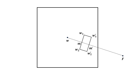
Figure 7: The region encompassed by the rectangle $w_{1},w_{2},w_{1}^{\prime},w_{2}^{\prime}$ is known as $A$. $d(w,m)=r/4$, $d(m,m^{\prime})=r/8$, and $d(m,w_{1})=d(m,w_{2})=r/8$.

Notice that all points within the rectangle lie within a distance of $r/2$ from $w$ and hence the entire region of the rectangle lies within $B_{w}(r)$. Call this region $A$. Since the area of $A$ is a constant fraction of $B_{w}(r)$ ($A$ is at least $1/32$ of the area of $B_{w}(r)$) and $w$ has $\Omega(\log n)$ neighbors on expectation in $B_{w}(r)$, we see that with high probability, there is at least one neighbor of $w$, call it $w^{\prime}$ in $A$.

Now, we want to upper bound the distance $d(w^{\prime},F)$, assuming $w^{\prime}$ is some point in $A$. Recall that the algorithm has $w$ forward the message to its neighbor $v$ that is closest (by Euclidean distance) to $F$. As such, the distance $d(w^{\prime},F)$ acts as an upper bound on the actual distance $d(v,F)$.

Now, notice that within $A$, the worst possible location for $w^{\prime}$ (resulting in the largest value of $d(w^{\prime},F)$) is when $w^{\prime}$ is either $w_{1}$ or $w_{2}$. In such a situation,

$$d(w^{\prime},F) \leq d(w^{\prime},m)+d(m,F)\hbox{ by the triangle inequality}$$

$$=r/8+d(w,F)-r/4\hbox{ since $d(w,F)\geq r/4$}$$

$$\leq d(w,F)-r/8.$$

Using Lemma 3.12, we prove the following lemma.

Lemma 3.14.

Within $O(1)$ hops in $G(1)$, using Algorithm 2, there exists a node $u$ that is reachable from $S$ such that $F$ lies within $B_{u}(r)$.

Proof 3.15.

From Lemma 3.12, we see that until the message reaches a node $u$ such that $F$ lies within $B_{u}(r)$, the distance to $F$ (from the current node) decreases by at least $r/8$ every time the message is forwarded to a new node. More formally, if the message is currently at node $w$, and $w^{\prime}$ is chosen as per 2 such that $F$ does not lie within $B_{w^{\prime}}(r)$, then $d(w^{\prime},F)\leq d(w,F)-r/8$. Since $d(S,F)\leq\sqrt{2}$ and $r$ is a constant, we see that in $\lceil 8\sqrt{2}/r\rceil=O(1)$ hops, we reach a node $u$ such that $F$ lies within $B_{u}(r)$.

The above lemma shows that it takes $O(1)$ hops using $G(1)$ for a message to travel from $S$ to $u$. However, these are upper bounds on the number of hops taken by the greedy approach. If there exists a shorter path (e.g. via $G(0)$), both in hops and by extension propagation cost, from $S$ to some node $u^{\prime}$ that satisfies the property that $F$ lies within $B_{u^{\prime}}(r)$, that path will be taken instead.

The following two lemmas show that, once the message has reached node $u$ from Lemma 3.14, the algorithm can find a path to $F$ using at most $O(1)$ edges from each of the graphs $G(i)$, $2\leq i\leq\kappa$. The proof of the following lemmas is a straightforward generalization of the proofs of Lemma 3.12 and Lemma 3.14.

Lemma 3.16.

If the message is currently at node $u$ such that $F$ lies within $B_{u}(r^{i})$ but outside $B_{u}(r^{i+1})$, and the node that the message is forwarded to via Algorithm 2 is some $u^{\prime}$, then $d(u^{\prime},F)\leq d(u,F)-r^{i+1}/8$.

Lemma 3.17.

For a node $u$ and some value of $i$, $1\leq i<\kappa$, such that $F$ lies within $B_{u}(r^{i})$ but outside $B_{u}(r^{i+1})$, within $O(1)$ hops in $G(i+1)$, using Algorithm 2, there exists a node $u^{\prime}$ that is reachable from $u$ such that $F$ lies within $B_{u^{\prime}}(r^{i+1})$.

Recall that for every node $u$, all of the nodes that lie within $B_{u}(r^{\kappa})$ are neighbors of $u$ in $G(\kappa)$. Thus, once a node $v$ is reached such that $F$ lies within $B_{u}(r^{\kappa})$, the message can be directly forwarded to $F$ as $F$ is a neighbor of $v$ in $G(\kappa)$. Thus, we see that Algorithm 2 results in the message being routed from $S$ to $F$. Each subgraph is used to route the message for $O(1)$ hops and there are $\kappa$ such subgraphs. Thus, we have the following lemma.

Lemma 3.18.

Consider the graph $G^{*}$ obtained at the end of Algorithm 1. For any source node $S$ and any destination node $F$, routing a packet from $S$ to $F$ using 2 takes $O\mathchoice{\left(\kappa\right)}{(\kappa)}{(\kappa)}{(\kappa)}$ hops.

Now we argue about the propagation cost of the path taken to route the message from $S$ to $F$.

Lemma 3.19.

Consider the graph $G^{*}$ obtained at the end of Algorithm 1. For any source node $S$ and any destination node $F$, the propagation cost of the routed path from $S$ to $F$ due to Algorithm 2 is $O(d(S,F))$, where $d(S,F)$ is the Euclidean distance between $S$ and $F$.

Proof 3.20.

It is either the case that (i) $F$ lies outside $B_{S}(r)$, (ii) $F$ lies within $B_{S}(r^{i})$ but outside $B_{S}(r^{i+1})$ for some $1\leq i<\kappa$, or (iii) $F$ lies in $B_{S}(r^{\kappa})$. We analyze each case separately and show that in each case, the propagation cost is $O(d(S,F))$.

Case (i) $F$ lies outside $B_{S}(r)$: If $F$ lies outside $B_{S}(r)$, then $SF\geq r$. From Lemma 3.14 and Lemma 3.17, we see that the message travels at most a constant number of hops in each $G(i)$, $1\leq i\leq\kappa$. Let $c$ be the largest constant among all such constants. Consider a straight line drawn from $S$ to $F$. Each of the at most $c$ hops in $G(i)$, $1\leq i\leq\kappa$, say between some nodes $u$ and $v$ in $G(i)$ results in an at most $\sqrt{2}r^{i}$ additional cost to the propagation cost. Thus, the total propagation cost in a path taken by the message is $\leq c\sqrt{2}\sum_{j=1}^{\kappa}r^{j}\leq c\sqrt{2}r/(1-r)=O(d(S,F))$.

Case (ii) $F$ lies within $B_{S}(r^{i})$ but outside $B_{S}(r^{i+1})$ for some $1\leq i<\kappa$: If $F$ lies outside $B_{S}(r^{i+1})$ for some $1\leq i<\kappa$, then $SF\geq r^{i+1}$. Using a similar analysis to Case (i), we see that the total propagation cost in a path taken by the message is $\leq c\sqrt{2}\sum_{j=i+1}^{\kappa}r^{j}\leq c\sqrt{2}r^{i+1}/(1-r)=O(d(S,F))$.

Case (iii) $F$ lies in $B_{S}(r^{\kappa})$: If $F$ lies within $B_{S}(r^{\kappa})$, then $F$ is an immediate neighbor of $S$ and as such, the propagation cost of the path is exactly $d(S,F)$.

From Lemma 3.18 and Lemma 3.19, we arrive at our main theorem.

Theorem 3.21.

Consider the graph $G^{*}$ obtained at the end of Algorithm 1. For any source node $S$ and any destination node $F$, routing a packet from $S$ to $F$ using Algorithm 2 takes $O(\log n)$ hops and the propagation cost of the routed path is $O(d(S,F))$, where $d(S,F)$ is the Euclidean distance between $S$ and $F$.

4 Conclusion and Future Work

We consider this work as a theoretical step towards the design and analysis of P2P topologies and associated communication protocols. While our theoretical framework is only a rough approximation to real-world P2P networks, it provides a rigorous model for the design and analysis of P2P protocols that takes into account propagation delays that depend on not only the graph topology but also on the distribution of nodes across the Internet. Our model is inspired by several studies on the Internet, particularly the Vivaldi system [12], which posits how nodes on the Internet can be assigned coordinates in a low-dimensional, even 2-dimensional, Euclidean space, that quite accurately captures the point-to-point latencies between nodes. We have additionally performed empirical research, via simulation, on the Bitcoin P2P network that suggests that the model is a reasonable approximation to a real-world P2P network. We have also performed preliminary simulations of our routing and broadcast protocols which broadly support our theoretical bounds. We leave a detailed experimental study for future work.

References

- [1] Ittai Abraham, Dahlia Malkhi, and Oren Dobzinski. LAND: stretch (1 + epsilon) locality-aware networks for dhts. In J. Ian Munro, editor, Proceedings of the Fifteenth Annual ACM-SIAM Symposium on Discrete Algorithms, SODA 2004, New Orleans, Louisiana, USA, January 11-14, 2004, pages 550–559. SIAM, 2004. URL: http://dl.acm.org/citation.cfm?id=982792.982873.
- [2] D. Aldous and J.M. Steele. Asymptotics for euclidean minimal spanning trees on random points. Probab. Th. Rel. Fields, (92):247–258, 1992.
- [3] Dana Angluin, James Aspnes, Jiang Chen, Yinghua Wu, and Yitong Yin. Fast construction of overlay networks. In Phillip B. Gibbons and Paul G. Spirakis, editors, SPAA 2005: Proceedings of the 17th Annual ACM Symposium on Parallelism in Algorithms and Architectures, July 18-20, 2005, Las Vegas, Nevada, USA, pages 145–154. ACM, 2005. doi:10.1145/1073970.1073991.
- [4] John Augustine, Gopal Pandurangan, and Peter Robinson. Fast byzantine agreement in dynamic networks. In Proceedings of the ACM Symposium on Principles of Distributed Computing (PODC), pages 74–83, 2013.
- [5] John Augustine, Gopal Pandurangan, Peter Robinson, Scott Roche, and Eli Upfal. Enabling robust and efficient distributed computation in dynamic peer-to-peer networks. In IEEE 56th Annual Symposium on Foundations of Computer Science (FOCS), pages 350–369, 2015.
- [6] John Augustine, Gopal Pandurangan, Peter Robinson, and Eli Upfal. Towards robust and efficient computation in dynamic peer-to-peer networks. In Proceedings of the Twenty-third Annual ACM-SIAM Symposium on Discrete Algorithms (SODA), pages 551–569, 2012.
- [7] Amitabha Bagchi, Ankur Bhargava, Amitabh Chaudhary, David Eppstein, and Christian Scheideler. The effect of faults on network expansion. Theory Comput. Syst., 39(6):903–928, 2006. doi:10.1007/s00224-006-1349-0.
- [8] Free BSD. ping(8), 2022. URL: https://man.freebsd.org/cgi/man.cgi?query=ping&sektion=8.
- [9] Colin Cooper, Martin E. Dyer, and Catherine S. Greenhill. Sampling regular graphs and a peer-to-peer network. In Proceedings of the Sixteenth Annual ACM-SIAM Symposium on Discrete Algorithms (SODA), pages 980–988. SIAM, 2005.
- [10] Colin Cooper, Martin E. Dyer, and Catherine S. Greenhill. Sampling regular graphs and a peer-to-peer network. Combinatorics, Probability & Computing, 16(4):557–593, 2007.
- [11] Kyle Croman, Christian Decker, Ittay Eyal, Adem Efe Gencer, Ari Juels, Ahmed Kosba, Andrew Miller, Prateek Saxena, Elaine Shi, Emin Gün Sirer, Dawn Song, and Roger Wattenhofer. On scaling decentralized blockchains. In Jeremy Clark, Sarah Meiklejohn, Peter Y.A. Ryan, Dan Wallach, Michael Brenner, and Kurt Rohloff, editors, Financial Cryptography and Data Security, pages 106–125, Berlin, Heidelberg, 2016. Springer Berlin Heidelberg.
- [12] Frank Dabek, Russ Cox, M. Frans Kaashoek, and Robert Tappan Morris. Vivaldi: a decentralized network coordinate system. In Raj Yavatkar, Ellen W. Zegura, and Jennifer Rexford, editors, ACM SIGCOMM, pages 15–26, 2004.
- [13] Maximilian Drees, Robert Gmyr, and Christian Scheideler. Churn- and dos-resistant overlay networks based on network reconfiguration. In Christian Scheideler and Seth Gilbert, editors, Proceedings of the 28th ACM Symposium on Parallelism in Algorithms and Architectures, SPAA 2016, Asilomar State Beach/Pacific Grove, CA, USA, July 11-13, 2016, pages 417–427. ACM, 2016. doi:10.1145/2935764.2935783.
- [14] Tobias Friedrich, Thomas Sauerwald, and Alexandre Stauffer. Diameter and broadcast time of random geometric graphs in arbitrary dimensions. Algorithmica, 67(1):65–88, 2013.
- [15] Ghurumuruhan Ganesan. Stretch and diameter in random geometric graphs. Algorithmica, 80:300–330, 2018.
- [16] Seth Gilbert, Gopal Pandurangan, Peter Robinson, and Amitabh Trehan. Dconstructor: Efficient and robust network construction with polylogarithmic overhead. In Yuval Emek and Christian Cachin, editors, PODC ’20: ACM Symposium on Principles of Distributed Computing, Virtual Event, Italy, August 3-7, 2020, pages 438–447. ACM, 2020. doi:10.1145/3382734.3405716.
- [17] C. Gkantsidis, M. Mihail, and A. Saberi. Random walks in peer-to-peer networks: Algorithms and evaluation. Performance Evaluation, 63(3):241–263, 2006.
- [18] Thorsten Götte, Kristian Hinnenthal, Christian Scheideler, and Julian Werthmann. Time-optimal construction of overlay networks. In Avery Miller, Keren Censor-Hillel, and Janne H. Korhonen, editors, ACM Symposium on Principles of Distributed Computing (PODC), pages 457–468, 2021.
- [19] Kirsten Hildrum, John Kubiatowicz, Sean Ma, and Satish Rao. A note on the nearest neighbor in growth-restricted metrics. In J. Ian Munro, editor, Proceedings of the Fifteenth Annual ACM-SIAM Symposium on Discrete Algorithms, SODA 2004, New Orleans, Louisiana, USA, January 11-14, 2004, pages 560–561. SIAM, 2004. URL: http://dl.acm.org/citation.cfm?id=982792.982874.
- [20] Shlomo Hoory, Nathan Linial, and Avi Wigderson. Expander graphs and their applications. Bulletin of the American Mathematical Society, 43(4):439–561, 2006.
- [21] Zi Hu, John S. Heidemann, and Yuri Pradkin. Towards geolocation of millions of IP addresses. In Proceedings of the 12th ACM SIGCOMM Internet Measurement Conference, IMC, pages 123–130, 2012.
- [22] Tim Jacobs and Gopal Pandurangan. Stochastic analysis of a churn-tolerant structured peer-to-peer scheme. Peer-to-Peer Networking and Applications, 6(1):1–14, 2013.
- [23] David R. Karger and Matthias Ruhl. Finding nearest neighbors in growth-restricted metrics. In John H. Reif, editor, Proceedings on 34th Annual ACM Symposium on Theory of Computing, May 19-21, 2002, Montréal, Québec, Canada, pages 741–750. ACM, 2002. doi:10.1145/509907.510013.
- [24] Brad Karp and Hsiang-Tsung Kung. Gpsr: Greedy perimeter stateless routing for wireless networks. In Proceedings of the 6th annual international conference on Mobile computing and networking, pages 243–254, 2000.
- [25] Evangelos Kranakis, Harvinder Singh, and Jorge Urrutia. Compass routing on geometric networks. In Proceedings of the 11th Canadian Conference on Computational Geometry, UBC, Vancouver, British Columbia, Canada, August 15-18, 1999, 1999. URL: http://www.cccg.ca/proceedings/1999/c46.pdf.
- [26] Mike Krebs and Anthony Shaheen. Expander families and Cayley graphs: a beginner’s guide. Oxford University Press, 2011.
- [27] Fabian Kuhn, Roger Wattenhofer, Yan Zhang, and Aaron Zollinger. Geometric ad-hoc routing: Of theory and practice. In Proceedings of the twenty-second annual symposium on Principles of distributed computing, pages 63–72, 2003.
- [28] C. Law and K.-Y. Siu. Distributed construction of random expander networks. In IEEE INFOCOM, pages 2133 – 2143, 2003.
- [29] Peter Mahlmann and Christian Schindelhauer. Distributed random digraph transformations for peer-to-peer networks. In Proceedings of the Eighteenth Annual ACM Symposium on Parallelism in Algorithms and Architectures (SPAA), pages 308–317, 2006.
- [30] Yifan Mao, Soubhik Deb, Shaileshh Bojja Venkatakrishnan, Sreeram Kannan, and Kannan Srinivasan. Perigee: Efficient peer-to-peer network design for blockchains. In ACM Symposium on Principles of Distributed Computing (PODC), pages 428–437, 2020.
- [31] Andrew K. Miller, James Litton, Andrew Pachulski, Neal Gupta, Dave Levin, Neil Spring, and Bobby Bhattacharjee. Discovering bitcoin ’ s public topology and influential nodes. 2015.
- [32] Michael Mitzenmacher and Eli Upfal. Probability and Computing: Randomized Algorithms and Probabilistic Analysis. Cambridge University Press, edition, 2017.
- [33] S. Muthukrishnan and Gopal Pandurangan. Thresholding random geometric graph properties motivated by ad hoc sensor networks. J. Comput. Syst. Sci., 76(7):686–696, 2010.
- [34] Edgar M. Palmer. Graphical Evolution: An Introduction to the Theory of Random Graphs. John Wiley & Sons, Inc., USA, 1985.
- [35] Gopal Pandurangan, Prabhakar Raghavan, and Eli Upfal. Building low-diameter P2P networks. In IEEE Symposium on the Foundations of Computer Science (FOCS), pages 492–499, 2001.
- [36] Gopal Pandurangan, Peter Robinson, and Amitabh Trehan. Dex: self-healing expanders. Distributed Computing, 29(3):163–185, 2016.
- [37] David Peleg. Distributed Computing: A Locality-Sensitive Approach. Society for Industrial and Applied Mathematics, 2000.
- [38] Mathew D. Penrose. Random Geometric Graphs. Oxford University Press, 2003.
- [39] C. Greg Plaxton, Rajmohan Rajaraman, and Andréa W. Richa. Accessing nearby copies of replicated objects in a distributed environment. Theory Comput. Syst., 32(3):241–280, 1999. doi:10.1007/s002240000118.
- [40] Antony Rowstron and Peter Druschel. Pastry: Scalable, decentralized object location, and routing for large-scale peer-to-peer systems. In Middleware 2001: IFIP/ACM International Conference on Distributed Systems Platforms Heidelberg, Germany, November 12–16, 2001 Proceedings 2, pages 329–350. Springer, 2001.
- [41] Atish Das Sarma, Anisur Rahaman Molla, and Gopal Pandurangan. Distributed computation in dynamic networks via random walks. Theor. Comput. Sci., 581:45–66, 2015. doi:10.1016/j.tcs.2015.02.044.
- [42] Atish Das Sarma, Danupon Nanongkai, Gopal Pandurangan, and Prasad Tetali. Distributed random walks. J. ACM, 60(1):2:1–2:31, 2013. doi:10.1145/2432622.2432624.