Almost sure convergence of stochastic Hamiltonian descent methods

Abstract.

Gradient normalization and soft clipping are two popular techniques for tackling instability issues and improving convergence of stochastic gradient descent (SGD) with momentum. In this article, we study these types of methods through the lens of dissipative Hamiltonian systems. Gradient normalization and certain types of soft clipping algorithms can be seen as (stochastic) implicit-explicit Euler discretizations of dissipative Hamiltonian systems, where the kinetic energy function determines the type of clipping that is applied. We make use of unified theory from dynamical systems to show that all of these schemes converge almost surely to stationary points of the objective function.

1. Introduction

In this article we consider the optimization problem

(1) $$\min_{q\in\mathbb{R}^{d}}F(q),$$

where $F:\mathbb{R}^{d}\to\mathbb{R}$ is an objective function. A common setting in mathematical statistics and machine learning is that $F$ is a weighted sum of loss functions

(2) $$F(q)=\frac{1}{N}\sum_{i=1}^{N}\ell(h(x_{i},q),y_{i}).$$

Here, $\{(x_{i},y_{i})\}_{i=1}^{N}$ is an underlying data set of feature-label pairs in the feature-label space $\mathcal{X}\times\mathcal{Y}$, $h(q,\cdot)$ is a model with model parameters $q$ such as a neural network or a regression function, and $\ell$ is a loss function. A common approach within the machine learning community for solving problems of the type (1) is to employ stochastic gradient descent (SGD) (Robbins and Monro, 1951). The solution to (1) is approximated iteratively with a stochastic approximation to the gradient of (2):

(3) $$q_{k+1}=q_{k}-\alpha_{k}\nabla f(q_{k},\xi_{k}).$$

Here $\alpha_{k}$ is the learning rate and $\xi_{k}$ is a random variable that accounts for the stochasticity. A common choice is to take a random subset $B_{\xi_{k}}\subset\{1,\dots,N\}$ of the indices of (2) and choose

$$\nabla f(q,\xi_{k})=\frac{1}{|B_{\xi_{k}}|}\sum_{i\in B_{\xi_{k}}}\nabla\ell(h(x_{i},q),y_{i})),$$

where $|B_{\xi_{k}}|$ denotes the cardinality of $B_{\xi_{k}}$. This is attractive when $N$ is very large and $|B_{\xi}|\ll N$, as it is less computationally expensive than gradient descent. It also tends to escape local saddle points (Fang et al., 2019) - an appealing property as many machine learning problems are non-convex. Among the variations of SGD is the popular SGD with momentum. Its deterministic counterpart was first introduced in the seminal work of Polyak (1964). A common form of this algorithm is expressed as an update in two stages

(4) $$\begin{split}p_{k+1}&=\beta_{k}p_{k}-\alpha_{k}\nabla f(q_{k},\xi_{k})\\ q_{k+1}&=q_{k}+\alpha_{k}p_{k+1}\end{split}$$

where $p_{0}=0$ and $\beta_{k}>0$ is a momentum parameter. The usage of the momentum update makes the algorithm less sensitive to noise. Indeed, by an iterative argument, we obtain that

$$p_{k+1}=-\sum_{i=0}^{k}\left(\prod_{j=i+1}^{k}\beta_{j}\right)\alpha_{i}\nabla f(q_{i},\xi_{k}).$$

That is, $p_{k+1}$ is an average of the previous gradients where $\beta_{k}$ determines how much we value information from the preceding stages.

Notwithstanding the benefits of stochastic gradient algorithms, they frequently suffer from instability problems such as exploding gradients (Pascanu et al., 2013; Bengio et al., 1994) and sensitivity to the choice of learning rate (Owens and Filkin, 1989). A way to mitigate these issues is to employ gradient clipping (Goodfellow et al., 2016; Pascanu et al., 2012) or gradient normalization. Gradient normalization was introduced in Poljak (1967) in the deterministic and a stochastic version appears already in Andradóttir (1990). A normalized version of (3) is given by

$$q_{k+1}=q_{k}-\alpha_{k}\frac{\nabla f(q_{k},\xi_{k})}{\lVert\nabla f(q_{k},\xi_{k})\rVert_{2}}.$$

In practice a small number $\epsilon>0$ is added in the denominator to ensure that the update does not become infinitely large.

Gradient clipping was first introduced in Mikolov (2013). In so-called hard clipping, the gradient is simply rescaled if it is larger than some predetermined threshold. Soft clipping, on the other hand, makes use of a differentiable function for rescaling the gradient (Zhang et al., 2020a). It was recently shown that hard clipping algorithms suffer from an unavoidable bias term (Koloskova et al., 2023); a term in the convergence bound that does not decrease as the number of iterations increases. This is one reason why soft clipping is preferable.

1.1. Gradient normalization, momentum and Hamiltonian systems

In this article, we study gradient normalization and soft clipping of stochastic momentum algorithms from the perspective of Hamiltonian systems. As a first step, we note that if we take $\beta_{k}=1-\gamma\alpha_{k}$ with $\gamma>0$, we can view (4) as an approximate implicit-explicit Euler discretization of the equation system

(5) $$\begin{split}\dot{p}&=-\nabla F(q)-\gamma p,\\ \dot{q}&=p.\end{split}$$

The system (5) is nearly Hamiltonian (Glendinning, 1994); taking

(6) $$H(p,q)=F(q)+\varphi(p),$$

with $\varphi(p)=\frac{1}{2}\lVert p\rVert_{2}^{2}$, we can write it on the form

(7) $$\begin{split}\dot{p}&=-\nabla_{q}H(p,q)-\nabla_{\dot{q}}\mathcal{R}(\dot{q}),\\ \dot{q}&=\nabla_{p}H(p,q),\end{split}$$

where $\nabla_{p},\nabla_{q}$ denote the gradients with respect to $p$ and $q$ respectively and $\mathcal{R}(\dot{q})=\gamma\frac{\lVert\dot{q}\rVert_{2}^{2}}{2}$ is a Rayleigh dissipation function that accounts for energy dissipation (viscous friction) of the system. Note that this choice of $\mathcal{R}$ yields $\nabla_{\dot{q}}\mathcal{R}(\dot{q})=\gamma\nabla_{p}H(p,q)$, which will always be the case in this paper. Thus, for a Hamiltonian of the form (6), equation (7), reads

$$\begin{split}\dot{p}&=-\nabla F(q)-\gamma\nabla\varphi(p),\\ \dot{q}&=\nabla\varphi(p).\end{split}$$

We notice that any fixed point of this system is a stationary point of $F$, since $(\dot{q},\dot{p})=0$ implies that $\nabla F(q)=0$. The dissipation term is often included as an extra term in the Euler-Lagrange equations

$$\nabla_{\dot{q}}L(q,\dot{q})-\frac{\mathrm{d}}{\mathrm{d}t}L(q,\dot{q})=\nabla_{\dot{q}}\mathcal{R}(\dot{q}),$$

where $L(q,\dot{q})=\varphi^{*}(\dot{q})-F(q)$ is the Lagrangian, and $\varphi^{*}$ is the convex conjugate of $\varphi$, compare Proposition 51.2 and Ex. 51.3 in Zeidler (1985). The physical interpretation is that $q$ is the position of a particle in a potential field $F(q)$ with kinetic energy given by $\varphi^{*}(\dot{q})$ (in the case when $\varphi(p)=\frac{\lVert p\rVert_{2}^{2}}{2}$ we have $\varphi^{*}(\dot{q})=\frac{\lVert\dot{q}\rVert_{2}^{2}}{2}$). In many scenarios, such as in this case, it happens that the friction tern is proportional to the velocity (Goldstein et al., 2014). A ball rolling on a rough incline (Wolf et al., 1998; Bideau et al., 1994)) or on a tilted plane coated with a viscous fluid (Bico et al., 2009) could for instance be modelled in this fashion, giving weight to the analogy of the heavy ball (Polyak, 1964). See also Goodfellow et al. (2016), for a further discussion on this.

We additionally note that the $H(p,q)$ is decreasing along the paths of (7) since

(8) $$\frac{\mathrm{d}}{\mathrm{d}t}H(p(t),q(t))=-\gamma\lVert\nabla_{p}H(p,q)\rVert_{2}^{2}\leq 0.$$

Under the assumption that $F$ is differentiable and coercive, this implies that the sublevel sets $M_{c}=\{(p,q):H(p,q)\leq c\}$ are compact. LaSalle’s invariance theorem (LaSalle, 1960) now implies that all solutions with initial conditions in $M_{c}$ tends to a stationary point of $F$. In this paper, we consider generalizations of the scheme (4) to equations of the type (7) where $F$ is an $L$-smooth, coercive function and $\varphi$ is a convex, coercive and $L$-smooth function. The scheme we consider is given by

(9) $$\begin{split}p_{k+1}&=p_{k}-\alpha_{k}\nabla f(q_{k},\xi_{k})-\alpha_{k}\gamma\nabla\varphi(p_{k}),\\ q_{k+1}&=q_{k}+\alpha_{k}\nabla\varphi(p_{k+1}),\end{split}$$

where $p_{0}=0$, $q_{0}$ is arbitrary, and $\{\xi_{k}\}_{k\geq 0}$ is a sequence of independent, identically distributed random variables. We show that this scheme converges almost surely to the set of stationary points of $F$. If we take $\varphi(x)=\frac{\lVert x\rVert_{2}^{2}}{2}$ in (9), we get (4). Taking $\varphi(x)=\sqrt{\lVert x\rVert_{2}^{2}+\epsilon},\ \epsilon>0$, gives us a gradient normalization scheme, where both the gradient and the momentum variables are rescaled:

(10) $$\begin{split}p_{k+1}&=p_{k}-\alpha_{k}\nabla f(q_{k},\xi_{k})-\alpha_{k}\gamma\frac{p_{k}}{\sqrt{\lVert p_{k}\rVert_{2}^{2}+\epsilon}},\\ q_{k+1}&=q_{k}+\alpha_{k}\frac{p_{k+1}}{\sqrt{\lVert p_{k+1}\rVert_{2}^{2}+\epsilon}}.\end{split}$$

Other conceivable choices are

1. Relativistic kinetic energy: $\varphi(x)=c\sqrt{\lVert x\rVert_{2}^{2}+(mc)^{2}}$. (Franca et al., 2020)

2. Non-relativistic kinetic energy: $\varphi(x)=\frac{1}{2}\langle x,Ax\rangle+\langle b,x\rangle+c$, where $A$ is a positive definite, symmetric matrix, $b\in\mathbb{R}^{d}$ and $c\in\mathbb{R}$. (Goldstein et al., 2014)

3. Gradient rescaling: $\varphi(x)=c\sqrt{\lVert x\rVert_{2}^{2}+\epsilon}$, for $c,\epsilon>0$.

4. Soft clipping: $\varphi(x)=\sqrt{1+\lVert x\rVert_{2}^{2}}$.

5. The symmetric LogSumExp-function: $\varphi(x)=\ln\left(\sum_{i=1}^{d}e^{x_{i}}+e^{-x_{i}}\right)$, which can be seen as an approximation of the $\ell^{\infty}$-norm (Sherman, 2013).

6. Half-squared $\ell^{p}$-norm: $\varphi(x)=\frac{1}{2}\lVert x\rVert_{p}^{2}$, for $p\in[2,\infty)$.

Examples i), iii) and iv) are analytically similar, but give rise to different behaviours in (9). We refer the reader to Beck (2017); Peressini et al. (1993), for verifying that the functions above satisfy the assumptions in Section 4.2.

2. Related works

We here briefly discuss some results that are related to the analysis in this paper. In the first section we discuss other formulations of SGD with momentum and how the formulation in this paper relates to them. In the second section we summarize work in optimization and statistics which make use of Hamiltonian dynamics. In the last section we discuss the approach we use for showing almost sure convergence of the methods.

2.1. Momentum algorithms

The implementations of SGD with momentum in the libraries Tensorflow (Abadi et al., 2015) and Pytorch (Paszke et al., 2019) are equivalent to (4) after a transformation of the learning rate:

$$\begin{split}p_{k+1}&=\beta_{k}p_{k}-\alpha_{k}\nabla f(q_{k},\xi_{k})\\ q_{k+1}&=q_{k}+p_{k+1}.\end{split}$$

Typically the momentum parameter $\beta_{k}$ is a fixed number. The update (4) resembles the (hard-clipped) algorithm proposed in Mai and Johansson (2021):

$$\begin{split}p_{k+1}&=\text{clip}_{r}\left((1-\beta_{k})p_{k}-\beta_{k}\nabla f(q_{k},\xi_{k})\right),\\ q_{k+1}&=q_{k}+\alpha_{k}p_{k+1},\end{split}$$

where $\text{clip}_{r}$ is a projection operator that projects the argument onto a ball of radius $r$ at the origin. The algorithm generated by (4) is also reminiscent of Stochastic Primal Averaging (SPA) (Defazio, 2021):

$$p_{k+1} =p_{k}-\eta_{k}\nabla f(q_{k},\xi_{k}),$$

$$q_{k+1} =(1-c_{k+1})q_{k}+c_{k+1}p_{k+1}.$$

In Theorem 1 in Defazio (2021) it is shown that this is equivalent to SGD with momentum version

$$p_{k+1} =\beta_{k}p_{k}+\nabla f(q_{k},\xi_{k}),$$

$$q_{k+1} =q_{k}-\alpha_{k}p_{k+1},$$

if one takes $\eta_{k+1}=\frac{\eta_{k}-\alpha_{k}}{\beta_{k+1}}$ and $c_{k+1}=\frac{\alpha_{k}}{\eta_{k}}$. The SPA algorithm can be seen as a randomized implicit-explicit Euler discretization of the equation system

$$\dot{p} =-\nabla F(q),$$

$$\dot{q} =p-q,$$

which after a change of variable is equivalent with (5) for $\gamma=1$.

Under the rather strong assumptions that the noise is almost surely bounded, so-called mixed-clipped SGD with momentum was studied in Zhang et al. (2020a):

$$p_{k+1} =\beta p_{k}-(1-\beta)\nabla f(q_{k},\xi_{k}),$$

$$q_{k+1} =q_{k}-\biggl{[}\nu\min\left(\eta,\frac{\gamma}{\lVert p_{k+1}\rVert_{2}}\right)p_{k+1}$$

$$+(1-\nu)\min\left(\eta,\frac{\gamma}{\lVert\nabla f(q_{k},\xi_{k})\rVert_{2}}\right)\nabla f(q_{k},\xi_{k})\biggr{]},$$

Here, $0\leq\nu\leq 1$ is an interpolation parameter.

A drawback with the previously mentioned analyses is that the convergence results are obtained in expectation, which means that there is no guarantee that a single path will converge.

2.2. Hamiltonian dynamics

Hamiltonian dynamics, in its energy conserving form, has been well-explored in the Markov chain Monte Carlo field, compare Leimkuhler and Matthews (2015). In Livingstone et al. (2017), various kinetic energy functions $\varphi$ are considered for equation (7) without the dissipation term $\nabla_{\dot{q}}\mathcal{R}(\dot{q})$.

The algorithm (9) was studied in the context of stochastic differential equations and Langevin dynamics in Stoltz and Trstanova (2018), where the noise is assumed to be Gaussian. In general, this is however a restrictive assumption in the stochastic optimization setting.

The specific update (10) bears resemblance to deterministic time integration- and optimization schemes studied in Franca et al. (2020), that arise as discretizations of the system

(11) $$\begin{split}\dot{p}&=-\nabla_{q}H(p,q)-\gamma p,\\ \dot{q}&=\nabla_{p}H(p,q),\end{split}$$

where the dissipation term $\gamma p$ emanates from Bateman’s Lagrangian $L(q,\dot{q})=e^{\gamma t}(\varphi^{*}(\dot{q})-F(q))$, see Bateman (1931). A similar point of view is also taken in Franca et al. (2021), but where so-called Bregman dynamics is employed. Similar to (8), one can show that a Hamiltonian on the form (6), with a convex kinetic energy function $\varphi$ is decreasing along the paths of (11). In the (deterministic) optimization setting this was studied in Maddison et al. (2018), where strictly convex kinetic energy functions $\varphi$ are considered. A stochastic gradient version is analysed in Kapoor and Harshvardhan (2021) for strongly convex objective functions $F$.

However, the stochastic optimization algorithm has not been studied for non-convex problems, and an analysis for merely convex (and not strictly convex) kinetic energy functions is lacking.

2.3. Almost sure convergence

The analysis in this paper is based on the ODE method, emanating from Ljung (1976). The particular proof strategy is due to Kushner and Clark (1978), and is based on linear interpolation of the sequence of iterates:

The basic idea is simply an extension of a compactness technique as used to construct solutions to ordinary differential equations. (Coddington and Levinson, 1984, pp. 42-45) (Kushner and Clark (1978))

The technique was extended to piecewise constant interpolations in Kushner and Yin (2003). The technique relies on the assumption that the iterates generated by the algorithm are finite almost surely; an assumption that has to be verified independently.

A similar analysis of the SGD with momentum was performed in Gadat et al. (2018). It was extended in Barakat et al. (2021), to a class of schemes that encompasses (4). The analytical approach is slightly different and does not cover the normalization- and clipping algorithms that we analyze in this article.

We also note that one can employ an analysis similar to that in e.g. Bottou et al. (2018), along with martingale results like that in Robbins and Siegmund (1971) to obtain almost sure convergence of a subsequence of the iterates. This is for instance the case in Sebbouh et al. (2021) where almost sure convergence guarantees of the type $\min_{0\leq k\leq K}\lVert\nabla F(q_{k})\rVert_{2}\to 0$ almost surely for SGD and SGD with momentum are established. These types of results are weaker than those obtained in this paper, since they cannot guarantee that the whole sequence of iterates $\{q_{k}\}_{k\geq 0}$ converges to a stationary point.

3. Contributions

Making use of Hamiltonian dynamics, we consider a large class of stochastic optimization algorithms (9) for large-scale optimization problems, for which we perform a rigorous convergence analysis. Our assumptions on the dissipation term $\varphi$ are fairly permissive, and thus the class of algorithms covers both interesting cases like normalized SGD with momentum and various soft-clipping methods with momentum, as well as novel methods. Our analysis shows that the iterates generated by any method in this class are finite almost surely, and that they converge almost surely to the set of stationary points of the objective function $F$. This means that the methods “always” work in practice, in contrast to what can be guaranteed by analyses that show convergence in expectation. These results are valid in many applications, due to fairly weak assumptions on the optimization problem. In particular, we do not assume any convexity of the objective function $F$.

4. Analysis

We first give a brief overview of the analysis in Section 4.1. In Section 4.2 we describe the setting and in Section 4.3 we give a more detailed outline of the theorems and the proofs. The proofs of the results are given in Appendix A.

4.1. Brief overview

The analysis is split into two parts. In the first, we show that the iterates generated by the scheme (9) converge almost surely under the assumption that they are bounded. We make use of a modification of the ODE method, compare Kushner and Yin (2003). Since the scheme is implicit-explicit, we cannot directly apply e.g. Theorem 2.1 in Kushner and Yin (2003).

Essentially, the idea is to

1. Introduce a pseudo time $t_{k}=\sum_{i=0}^{k-1}\alpha_{i}$.

2. Construct piecewise constant interpolations $P_{0}(t)$ and $Q_{0}(t)$ of $\{p_{k}\}_{k\geq 0}$ and $\{q_{k}\}_{k\geq 0}$ from (9).

3. Show that the time shifted processes $P_{k}(t)=P_{0}(t_{k}+t)$ and $Q_{k}(t)=Q_{0}(t_{k}+t)$ are equicontinuous in the extended sense (Kushner and Yin, 2003).

4. Show that $P_{k}(t)$ and $Q_{k}(t)$ asymptotically satisfies (7).

Making use of LaSalle’s invariance theorem (LaSalle, 1960), we can then conclude that $\{q_{k}\}_{k\geq 0}$ converges to the set of stationary points of $F$ almost surely.

In the second part, we show that the iterates of (9) are in fact finite almost surely, if the objective function $F$ and the convex kinetic energy function $\varphi$ are $L$-smooth and coercive. This is done by constructing a Lyapunov function with the help of the Hamiltonian $H$, and then appealing to the classical Robbins–Siegmund theorem (Robbins and Siegmund, 1971).

4.2. Setting

Let $(\Omega,\mathcal{F},\mathbb{P})$ be a probability space, and $\{\xi_{k}\}_{k\geq 0}$ be a sequence of independent, identically distributed random variables. We further let $\mathcal{F}_{k}$ denote the $\sigma-$algebra generated by $\xi_{0},\dots,\xi_{k-1}$. By $\mathbb{E}_{\xi_{k}}\left[X\right]$ we denote the conditional expectation of a random variable $X$ with respect to $\mathcal{F}_{k}$. We make the following assumptions on the stochastic gradients and the objective function $F$:

Assumption 1.

The stochastic gradient satisfies:

1. (Unbiasedness) $\mathbb{E}\left[\nabla f(x,\xi)\right]=\nabla F(x)$.

2. (Bounded variance) $\mathbb{V}\left[\nabla f(x,\xi)\right]\leq\sigma^{2}$,

where $\sigma\geq 0$ and $\mathbb{V}\left[\nabla f(x,\xi)\right]=\mathbb{E}\left[\lVert\nabla f(x,\xi)\rVert_{2}^{2}\right]-\lVert\nabla F(x)\rVert_{2}^{2}$.

Assumption 2.

The objective function $F$ is differentiable and satisfies:

1. (Lipschitz-continuous gradient) There is a constant $L>0$ such that $\lVert\nabla F(y)-\nabla F(x)\rVert_{2}\leq L\lVert x-y\rVert_{2}$, for all $x,y\in\mathbb{R}^{d}$.

2. (Coercivity) $\lim_{\lVert x\rVert_{2}\to\infty}F(x)=\infty$.

3. (Proper) There is a number $F_{*}>-\infty$ such that $F(x)\geq F_{*},\ \forall x\in\mathbb{R}^{d}$.

4. The set of critical points of $F$, $\{q:\nabla F(q)=0\}$ is bounded.

Assumption 2.ii) implies that the sublevel sets $\{x:F(x)\leq c\}$ are bounded, compare Proposition 11.12 in Bauschke and Combettes (2011). Assumption 2. i) implies $L$-smoothness:

$$F(y)-F(x)\leq\langle\nabla F(x),y-x\rangle+\frac{L}{2}\lVert x-y\rVert_{2}^{2},$$

for all $x,y\in\mathbb{R}^{d}$. These assumptions are fairly standard in the literature, but will not be applicable to every problem. In particular the differentiability and global Lipschitz-continuity might be problematic in certain applications. However, we find it highly likely that the analysis generalizes in several directions. Specifically, to the case where only a sub-differential exists, and to e.g. the case of “$(L_{0},L_{1})$-smoothness” as introduced by Zhang et al. (2020b). For simplicity, we consider only the case given by Assumptions 1 and 2.

We make the following assumptions of the kinetic energy function:

Assumption 3.

The kinetic energy function $\varphi$ is differentiable and satisfies:

1. (Lipschitz continuity of the gradient) There is a constant $\lambda>0$ such that $\lVert\nabla\varphi(y)-\nabla\varphi(x)\rVert_{2}\leq\lambda\lVert x-y\rVert_{2}$, for all $x,y\in\mathbb{R}^{d}$.

2. (Convexity) For all $x,y\in\mathbb{R}^{d}$, it holds that $\varphi(y)-\varphi(x)\leq\langle\nabla\varphi(y),y-x\rangle$.

3. (Coercivity) $\lim_{\lVert x\rVert_{2}\to\infty}\varphi(x)=\infty$.

4. (Proper) For all $x\in\mathbb{R}^{d}$, it holds that $\varphi(x)\geq\varphi_{*}>-\infty$.

Remark 4.1.

Asumption 2.ii), 2.iii), 3.iii) and 3.iv) together implies that the Hamiltonian $H(p,q)=F(q)+\varphi(p)$ is coercive as a function of $q$ and $p$.

The next restriction on the step size originates from Robbins and Monro (1951). Informally, the step sizes must go to zero in order to counter the stochasticity, but do so slowly enough that we have time to reach a stationary point.

Assumption 4 (Step sizes).

The step size sequence $\{\alpha_{k}\}_{k\geq 0}$ satisfies $\alpha_{0}=0$ and

1. $\sum_{k\geq 0}\alpha_{k}=\infty$.

2. $\sum_{k\geq 0}\alpha_{k}^{2}<\infty$.

In order to simplify the theorem statements, we finally consider the following assumption:

Assumption 5.

The sequences $\{p_{k}\}_{k\geq 0}$ and $\{q_{k}\}_{k\geq 0}$, generated by (9) are finite almost surely.

In Theorem 4.14, we will show that Assumption 5 holds when the other assumptions in this section are satisfied.

4.3. Outline of proof

The proofs of the results in this section can be found in Appendix A. The goal is to show an adaptation of Theorem 5.2.1 in Kushner and Yin (2003):

Theorem 4.2.

Let Assumptions 1, 2, 3, 4 and 5 hold and let the Hamiltonian $H$ be on the form (6). Define $A=\{z:\nabla H(z)=0\}$, with $z=(p,q)$ and let $\{z_{k}\}_{k\geq 0}=\{(p_{k},q_{k})\}_{k\geq 0}$, where $\{p_{k}\}_{k\geq 0}$ and $\{q_{k}\}_{k\geq 0}$ are given by (9). Then $z_{k}\to A$ almost surely:

(12) $$\lim_{k\to\infty}\inf_{a\in A}\lVert z_{k}-a\rVert_{\ell^{2}\left(\mathbb{R}^{2d}\right)}=0,\ \text{ a.s.}$$

In particular, this implies that $\{q_{k}\}_{k\geq 0}$ converges to the set of stationary points of $F$.

Closely following the analysis in Kushner and Yin (2003), we start with introducing a pseudo time $t_{k}=\sum_{i=0}^{k-1}\alpha_{i}$, and define two piecewise constant, (stochastic) interpolation processes defined by

(13) $$\begin{split}P_{0}(t)&=p_{0}I_{(-\infty,t_{0}]}(t)+\sum_{k=0}^{\infty}p_{k}I_{[t_{k},t_{k+1})}(t),\\ Q_{0}(t)&=q_{0}I_{(-\infty,t_{0}]}(t)+\sum_{k=0}^{\infty}p_{k}I_{[t_{k},t_{k+1})}(t).\end{split}$$

We next consider the shifted sequence of processes $\{P_{k}\}_{k\geq 0}$ and $\{Q_{k}\}_{k\geq 0}$, defined by

(14) $$\begin{split}P_{k}(t)&=P_{0}(t_{k}+t),\\ Q_{k}(t)&=Q_{0}(t_{k}+t).\end{split}$$

We note that $\{P_{k}\}_{k\geq 0}$ and $\{Q_{k}\}_{k\geq 0}$ are stochastic processes; they depend on $\omega\in\Omega$ through the stochasticity of the sequences $\{p_{k}\}_{k\geq 0}$ and $\{q_{k}\}_{k\geq 0}$. For brevity we will refrain from writing out the dependence on $\omega$.

The next step is to introduce the concept of extended equicontinuity (Kushner and Yin, 2003; Freise, 2016):

Definition 4.3 (Extended equicontinuity).

A sequence of $\mathbb{R}^{d}$-valued functions $\{f_{k}\}_{k\geq 0}$, defined on $(-\infty,\infty)$ , is said to be equicontinuous in the extended sense if $\{|f_{k}(0)|\}_{k\geq 0}$ is bounded and for every $T$ and $\epsilon>0$ there is $\delta>0$ such that

(15) $$\limsup_{k\to\infty}\sup_{0<|t-s|\leq\delta,\ t,s\in[0,T]}|f_{k}(t)-f_{k}(s)|\leq\epsilon.$$

Following Freise (2016), we show that the process $\{Z_{k}\}_{k\geq 0}=\{(P_{k},Q_{k})\}_{k\geq 0}$, where $\{P_{k}\}_{k\geq 0}$ and $\{Q_{k}\}_{k\geq 0}$ defined by (14), is equicontinuous in the extended sense:

Lemma 4.4 (Equicontinuous in the extended sense).

Consider $\{Z_{k}\}_{k\geq 0}=\{(P_{k},Q_{k})\}_{k\geq 0}$ where the sequences $\{P_{k}\}_{k\geq 0}$ and $\{Q_{k}\}_{k\geq 0}$ are defined by (14) (equivalently, by (19)). Suppose that $\{p_{k}\}_{k\geq 0}$ and $\{q_{k}\}_{k\geq 0}$ are defined by (9), that the Hamiltonian is on the form (6) and that Assumptions 1, 2, 3, 4 and 5 are satisfied. Then $\{Z_{k}\}_{k\geq 0}$ is equicontinuous in the extended sense, almost surely.

We can then appeal to the extended/discontinuous Arzelà–Ascoli theorem (Kushner and Yin, 2003; Freise, 2016; Droniou and Eymard, 2016), to conclude that $\{Z_{k}\}_{k\geq 0}$ has a subsequence that converges to a continuous function $z$:

Theorem 4.5 (Discontinuous Arzelà–Ascoli theorem).

Let $\{f_{k}\}_{k\geq 0}$ be a sequence of functions, defined on $\mathbb{R}^{d}$, that is equicontinuous in the extended sense. Then there is a subsequence $\{f_{n_{k}}\}_{n_{k}\geq 0}$ of $\{f_{k}\}_{k\geq 0}$, that converges uniformly on compact sets to a continuous function.

For a proof see, e.g. Theorem 6.2 in Droniou and Eymard (2016) or Theorem 12.3 in Billingsley (1968).

With this established, we proceed to show that $\{Z_{k}\}_{k\geq 0}$ is an asymptotic solution to (7); i.e. asymptotically $\{P_{k}\}_{k\geq 0}$ and $\{Q_{k}\}_{k\geq 0}$ satisfy (7). More precisely we show

Lemma 4.6 (Asymptotic solutions).

Let $\{P_{k}\}_{k\geq 0}$ and $\{Q_{k}\}_{k\geq 0}$ be defined by (14) (equivalently, by (19)). given the sequences $\{p_{k}\}_{k\geq 0}$ and $\{q_{k}\}_{k\geq 0}$ defined by (9). Further assume that Assumptions 1, 2, 3, 4 and 5 are satisfied. Then we can write

(16) $$\begin{split}P_{k}(t)=P_{k}(0)&-\int_{0}^{t}\nabla F(Q_{k}(s))\mathrm{d}s-\gamma\int_{0}^{t}\nabla\varphi(P_{k}(s))\mathrm{d}s+M_{k}(t)+\mu_{k}(t),\\ Q_{k}(t)=Q_{k}(0)&+\int_{0}^{t}\nabla\varphi(P_{k}(s))\mathrm{d}s+\nu_{k}(t)+\kappa_{k}(t),\end{split}$$

where the functions $\{M_{k}\}_{k\geq 0}$, $\{\mu_{k}\}_{k\geq 0}$, $\{\nu_{k}\}_{k\geq 0}$ and $\{\kappa_{k}\}_{k\geq 0}$ converge to $0$ uniformly on compact sets almost surely.

It follows that any limit point of $\{Z_{k}\}_{k\geq 0}$ satisfies

(17) $$\begin{split}P(t)&=P(0)-\int_{0}^{t}\nabla F(Q(s))\mathrm{d}s-\gamma\int_{0}^{t}\nabla\varphi(P(s))\mathrm{d}s\\ Q(t)&=Q(0)+\int_{0}^{t}\nabla\varphi(P(s))\mathrm{d}s.\end{split}$$

The limits we can extract by appealing to Theorem 4.5 are continuous. Thus it follows from (17) and the fundamental theorem of calculus that they are differentiable and satisfy (7).

Remark 4.7.

The functions $\{\mu_{k}\}_{k\geq 0}$ and $\{\nu_{k}\}_{k\geq 0}$ are essentially what is left when we have rewritten the sums in (13) as integrals. The functions $\{M_{k}\}_{k\geq 0}$ account for the difference between $\nabla F(q_{k})$ and $\nabla f(q_{k},\xi_{k})$ and $\kappa_{k}(t)$ for the implicit discretization in the second equation of (9).

Remark 4.8.

The convergence "uniformly on compact sets almost surely" is to be understood as uniformly on compact sets in $t$ and almost surely in $\omega$. For example we have for the sequence $\{M_{k}\}_{k\geq 0}$ that for any compact set $K\subset\mathbb{R}$ that

$$\lim_{k\to\infty}\sup_{t\in K}\lVert M_{k}(t)(\omega)\rVert_{2}=0,$$

for almost all $\omega\in\Omega$.

We now recall the definition of an invariant set (Kushner and Yin, 2003; Borkar, 2008):

Definition 4.9 (Invariant set).

An invariant set $\Lambda$ for the ODE (7) is a set such that for any $z_{0}\in\Lambda$, there is a solution $z(t)$ to (7) that lies entirely in $\Lambda$ (i.e. $z(t)\in\Lambda$, for all $-\infty<t<\infty$) and satisfies $z(0)=z_{0}$. It is positively invariant if $z_{0}\in\Lambda$ implies that $z(t)\in\Lambda$ for all $t\geq 0$.

By (8), it follows that the sublevel sets of the Hamiltonian are positively invariant; any solution to (7) starting in $M_{c}=\{(p,q):H(p,q)\leq c\}$ remains there for $t\geq 0$. We note that these sublevel sets are in fact equivalent to the $\delta-$neighborhoods of the set of stationary points, in the following sense:

Lemma 4.10.

Suppose that the Hamiltonian is of the form $H(p,q)=F(q)+\varphi(p)$ where $F$ and $\varphi$ satisfy Assumption 2 and 3. Let $A=\{z:\nabla H(z)=0\}$, where $z=(p,q)$ and for $\delta>0$ let $N_{\delta}(A)=\{z:\inf_{a\in A}\lVert z-a\rVert<\delta\}$. Introduce the Lyapunov function $V(z)=H(z)-F_{*}-\varphi_{*}$. Then $V(z)\geq 0$, has the same stationary points as $H$ and for every $\delta>0$ there is a $c\geq 0$ such that

$$\{x:V(x)<c\}=N_{\delta}(A),$$

i.e. the $\delta-$neighborhoods of $A$ can be taken to be the sublevel sets of the Lyapunov function $V$ and the former are positively invariant sets for the flow generated by (7).

A related concept is that of a locally asymptotically stable set (Borkar, 2008; Kushner and Yin, 2003):

Definition 4.11 (Locally asymptotically stable set).

A compact invariant set $M$ is called an attractor if it has an open neighbourhood $\mathcal{O}$ such that every trajectory in $\mathcal{O}$ remains in $\mathcal{O}$ and converges to $M$. The largest such $\mathcal{O}$ is called the domain of attraction of $M$. A compact invariant set $M$ is said to be Lyapunov stable if for any $\epsilon>0$, there exists a $\delta>0$ such that every trajectory initiated in the $\delta$-neighbourhood of $M$ remains in its $\epsilon$-neighbourhood. A compact invariant set $M$ is said to be asymptotically stable if it is both Lyapunov stable and an attractor.

With this in mind, we show the following lemma

Lemma 4.12.

Suppose that the Hamiltonian $H$ is differentiable and coercive. Then the set $A=\{(p,q):\nabla H(p,q)=0\}$ is a locally asymptotically stable set for (7) for which the domain of attraction is all of $\mathbb{R}^{d}\times\mathbb{R}^{d}$.

This will mean that the iterates $(p_{k},q_{k})$ visit any neighborhood of $A$ infinitely often, as formulated precisely in the next lemma:

Lemma 4.13.

Let the conditions of Theorem 4.2 hold and let $z_{k}=(p_{k},q_{k})$, where $p_{k}$ and $q_{k}$ are defined by (9). For every $\delta>0$ there is a subsequence of $\{z_{k}\}_{k\geq 0}$ which is contained in $N_{\delta}(A)$, the $\delta-$neighborhood of $A$.

The final step in proving Theorem 4.2 is then to show that the iterates cannot leave the neighborhoods of $A$ infinitely often. But since these neighborhoods are positively invariant by Lemma 4.10, the function $z$ which solves (7) cannot move away from them. The proof is therefore finished by carefully relating $z(t)$ and the iterates $z_{k}=(p_{k},q_{k})$.

To conclude the analysis, we demonstrate that under standard assumptions, it holds that the sequences $\{p_{k}\}_{k\geq 0}$ and $\{q_{k}\}_{k\geq 0}$ are finite almost surely:

Theorem 4.14 (Finiteness of $\{p_{k}\}_{k\geq 0}$ and $\{q_{k}\}_{k\geq 0}$).

Let the Hamiltonian be on the form (6) and let $\{p_{k}\}_{k\geq 0}$ and $\{q_{k}\}_{k\geq 0}$ be generated by (9). Further assume that Assumptions 1 to 4 hold. Then the sequences $\{p_{k}\}_{k\geq 0}$ and $\{q_{k}\}_{k\geq 0}$ are finite almost surely.

This leads to the following corollary to Theorem 4.2:

Corollary 4.15 (Convergence to a stationary point).

Let the assumptions of Theorem 4.14 be satisfied. Then $\{q_{k}\}_{k\geq 0}$ converges almost surely to the set of stationary points of the objective function $F$. If we additionally assume that the set of stationary points is finite, the convergence is to a unique equilibrium point.

5. Conclusion

In this paper, we have shown that the stochastic Hamiltonian descent algorithm (9), arising as a stochastic explicit-implicit Euler discretization of (7), under standard assumptions converges almost surely to the set of stationary points of the objective function $F$.

Appendix A Analysis

We start with rewriting the processes (14) on a form that is more reminiscent of the integral equations (17). As in Kushner and Yin [2003], we use the convention that

$$\begin{split}\sum_{i=n}^{k}a_{i}&=0,\ \text{ if }k=n-1\text{ (the empty sum)},\\ \sum_{i=n}^{k}a_{i}&=-\sum_{i=k+1}^{n-1}a_{i},\ \text{ if }k<n-1.\end{split}$$

By introducing the function

(18) $$m(t)=\begin{cases}j,\ t_{j}\leq t<t_{j+1},\\ 0,\ t\leq 0,\end{cases}$$

we can write (14) as

(19) $$\begin{split}P_{k}(t)&=p_{k}+\sum_{i=k}^{m(t_{k}+t)-1}(p_{i+1}-p_{i}),\\ Q_{k}(t)&=q_{k}+\sum_{i=k}^{m(t_{k}+t)-1}(q_{i+1}-q_{i}).\end{split}$$

Using the fact that $p_{k}=P_{k}(0)$ and $q_{k}=Q_{k}(0)$, along with the update (9), we can rewrite (19) as

(20) $$\begin{split}P_{k}(t)&=P_{k}(0)-\sum_{i=k}^{m(t_{k}+t)-1}\alpha_{i}\nabla F(q_{i})+M_{k}(t)-\gamma\sum_{i=k}^{m(t_{k}+t)-1}\alpha_{i}\nabla\varphi(p_{i}),\\ Q_{k}(t)&=Q_{k}(0)+\sum_{i=k}^{m(t_{k}+t)-1}\alpha_{i}\nabla\varphi(p_{i+1}),\end{split}$$

where

$$M_{k}(t)=\sum_{i=k}^{m(t_{k}+t)-1}\alpha_{i}\delta M_{i}$$

and $\delta M_{i}=\nabla f(q_{i},\xi_{i})-\nabla F(q_{i})$.

In the next section, we show that the process $\{M_{k}\}_{k\geq 0}$ converges uniformly on compact sets, almost surely, to $0$.

A.1. Convergence of the sequence $\{M_{k}\}$

The following lemma is from Kushner and Yin [2003]:

Lemma A.1 (Convergence of $\{M_{k}(t)\}_{k\geq 0}$).

The sequence $\{M_{k}(t)\}_{k\geq 0}$ converges uniformly on compact sets almost surely to $0$. More precisely, for any $T$ it holds that

(21) $$\lim_{k\to\infty}\sup_{t\in[0,T]}\lVert M_{k}(t)\rVert_{2}=0,$$

almost surely.

The proof is the same as in Kushner and Yin [2003] and is included for completeness.

Proof of Lemma A.1.

We let $\mathcal{F}_{j}=\sigma(\xi_{1},\dots,\xi_{j})$. By definition, we have that

$$M_{k}(t)=\sum_{i=k}^{m(t_{k}+t)-1}\alpha_{i}\delta M_{i},$$

where $\delta M_{i}=\nabla f(q_{i},\xi_{i})-\nabla F(q_{i})$. Define

$$\tilde{M}_{j}=\sum_{i=k}^{j}\alpha_{i}\delta M_{i}.$$

Then $\tilde{M}_{j}$ is a martingale sequence, i.e.

$$\mathbb{E}\left[\tilde{M}_{j+1}|\mathcal{F}_{j}\right]=\tilde{M}_{j},$$

and by Assumption 1.ii) it holds that

$$\mathbb{E}\left[\lVert\tilde{M}_{j+1}\rVert_{2}\right]<\infty,$$

compare Kushner and Yin [2003], Williams [1991]. We now show that (21) holds. For any interval $[0,T]$, we have that

$$\sup_{t\in[0,T]}\lVert M_{k}(t)\rVert_{2}=\sup_{k\leq j\leq l}\lVert\tilde{M}_{j}\rVert_{2},$$

where $l=m(t_{k}+T)$. By Doob’s submartingale inequality [Kushner and Yin, 2003, Williams, 1991], we have for every $\mu>0$ that

$$\mathbb{P}\left(\sup_{k\leq j\leq l}\lVert\tilde{M}_{j}\rVert_{2}\geq\mu\right)\leq\frac{\mathbb{E}\left[\lVert\tilde{M}_{l}\rVert_{2}^{2}\right]}{\mu^{2}}.$$

It holds that

$$\mathbb{E}\left[\lVert\tilde{M}_{l}\rVert_{2}^{2}\right] =\mathbb{E}\left[\lVert\sum_{i=k}^{l}\alpha_{i}\delta M_{i}\rVert_{2}^{2}\right]$$

$$=\mathbb{E}\left[\sum_{i=k}^{l}\alpha_{i}^{2}\lVert\delta M_{i}\rVert_{2}^{2}+2\sum_{i=k}^{l}\sum_{j=k}^{i-1}\alpha_{i}\alpha_{j}\langle\delta M_{i},\delta M_{j}\rangle\right]$$

$$=\mathbb{E}\left[\sum_{i=k}^{l}\alpha_{i}^{2}\lVert\delta M_{i}\rVert_{2}^{2}\right],$$

where we have used the fact that for $j<i$

$$\mathbb{E}\left[\langle\delta M_{i},\delta M_{j}\rangle\right]=\mathbb{E}\left[\mathbb{E}\left[\langle\delta M_{i},\delta M_{j}\rangle|\mathcal{F}_{j}\right]\right]=\mathbb{E}\left[\langle\mathbb{E}\left[\delta M_{i}|\mathcal{F}_{j}\right],\delta M_{j}\rangle\right]=0,$$

since $M_{j}$ is $\mathcal{F}_{j}$-measurable and $\mathbb{E}\left[\delta M_{i}|\mathcal{F}_{j}\right]=0$ (recall that $\xi_{i}$ is independent of $\mathcal{F}_{j}$). By Assumption 1.ii) we therefore have that

$$\mathbb{E}\left[\lVert\delta M_{i}\rVert_{2}^{2}\right]<\infty,$$

which implies that

$$\mathbb{P}\left(\sup_{k\leq j}\lVert\tilde{M}_{j}\rVert_{2}\geq\mu\right)\leq C\sum_{i=k}^{\infty}\alpha_{i}^{2}$$

and hence

$$\lim_{k\to\infty}\mathbb{P}\left(\sup_{k\leq j}\lVert\tilde{M}_{j}\rVert_{2}\geq\mu\right)=0.$$

By Theorem 1 in Section 2.10.3 of Shiryaev [2016], the sequence $\tilde{M}_{j}$ converges almost surely to $0$, i.e. there is a set $U$ such that $\mathbb{P}(U)=0$ and for every $\omega\in U^{c}$ we have that (21) holds. ∎

A.2. Equicontinuity of the sequences $\{P_{k}\}_{k\geq 0}$ and $\{Q_{k}\}_{k\geq 0}$

See 4.4 To show Lemma 4.4, we make use of an equivalent definition of extended equicontinuity:

Lemma A.2 (Equivalent definition of extended continuity).

A sequence of functions $\{f_{k}\}_{k\geq 0}$, $f_{k}:\mathbb{R}\to\mathbb{R}^{d}$ is equicontinuous in the extended sense if and only if $\{|f_{k}(0)|\}_{k\geq 0}$ is bounded and for every $T$ and $\epsilon>0$ there is a null sequence $\left(a_{k}\right)_{k\geq 0}$ (that is, $\lim_{k\to\infty}a_{k}=0$) such that

(22) $$\sup_{0<|t-s|\leq\delta,\ t,s\in[0,T]}|f_{k}(t)-f_{k}(s)|\leq\epsilon+a_{k}.$$

Proof of Lemma A.2.

By definition (15) is equal to

$$\lim_{k\to\infty}b_{k}\leq\epsilon$$

with

$$b_{k}:=\sup_{j\geq k}\sup_{0<|t-s|\leq\delta,\ t,s\in[0,T]}|f_{j}(t)-f_{j}(s)|.$$

Define

$$a_{k}=\max\{0,b_{k}-\epsilon\}.$$

Then $\left(a_{k}\right)_{k\geq 0}$ satisfies all the requirements; $a_{k}$ is clearly positive and by continuity of the function $\max\{0,x\}$ it holds that

$$\lim_{k\to\infty}a_{k}=\max\{0,\lim_{k\to\infty}b_{k}-\epsilon\}=0,$$

as $\lim_{k\to\infty}b_{k}-\epsilon\leq 0$. Furthermore, we have that

$$\sup_{0<|t-s|\leq\delta,\ t,s\in[0,T]}|f_{k}(t)-f_{k}(s)|\leq b_{k}\leq\epsilon+a_{k},$$

for every $k$ and thus we have shown that (22) follows from (15). We now show the converse. Suppose that (22) holds. Taking the supremum of (22) we obtain

$$\sup_{j\geq k}\sup_{0<|t-s|\leq\delta,t,s\in[0,T]}|f_{j}(t)-f_{j}(s)|\leq\epsilon+\sup_{j\geq k}a_{j}.$$

We finally take the limit with respect to $k$

$$\lim_{k\to\infty}\sup_{j\geq k}\sup_{0<|t-s|\leq\delta,\ t,s\in[0,T]}|f_{j}(t)-f_{j}(s)|\leq\epsilon+\lim_{k\to\infty}\sup_{j\geq k}a_{j}=:\epsilon+\limsup_{k\to\infty}a_{k}.$$

But as $\lim_{k\to\infty}a_{k}$ exists by assumption and is equal to $0$, we have that $\limsup_{k\to\infty}a_{k}=\lim_{k\to\infty}a_{k}=0$. We thus conclude that (15) holds. ∎

We now turn to the proof of Lemma 4.4.

Proof of Lemma 4.4.

Closely following Lemma 2 in Freise [2016]: We want to show that the sequence $\{Z_{k}\}_{k\geq 0}=\{(P_{k},Q_{k})\}_{k\geq 0}$, where $\{P_{k}\}_{k\geq 0}$ and $\{Q_{k}\}_{k\geq 0}$ are defined by (14), is equicontinuous in the extended sense.

First, we note that the sequences $\{P_{k}(0)\}$ and $\{Q_{k}(0)\}$ are finite except on a set of measure $0$, since by Assumption 5 $\sup_{k}\lVert p_{k}\rVert_{2}<\infty$ and $\sup_{k}\lVert q_{k}\rVert_{2}<\infty$ almost surely.

By Lemma A.2 an equivalent characterization of extended equicontinuity is that for every $\epsilon>0$, there is a sequence $\{a_{k}\}_{k\geq 0}$ such that $\lim_{k\to\infty}a_{k}=0$ and a $\delta>0$ such that

(23) $$\sup_{|t-s|<\delta,\ t,s\in[0,T]}\lVert Z_{k}(t)-Z_{k}(s)\rVert_{\ell^{2}\left(\mathbb{R}^{2d}\right)}\leq\epsilon+a_{k},\ \text{a.s.}$$

By (20), we have that

(24) $$\lVert P_{k}(t)-P_{k}(s)\rVert_{2}\leq C(\omega)\sum_{i=m(t_{k}+s)}^{m(t_{k}+t)-1}\alpha_{i}+\lVert M_{k}(t)\rVert_{2}+\lVert M_{k}(s)\rVert_{2},$$

where $C(\omega)=\sup_{i}\lVert\nabla F(q_{i})-\gamma\nabla\varphi(p_{i})\rVert_{2}$. By Assumption 5 along with the continuity of $\nabla F$ and $\nabla\varphi$, we have that $C(\omega)<\infty$, a.s. The sum on the right-hand side of (24) can be rewritten as

$$\sum_{i=m(t_{k}+s)}^{m(t_{k}+t)-1}\alpha_{i}=t_{m(t_{k}+t)}-t_{m(t_{k}+s)}.$$

By definition of $m$, (18), we have that

$$t_{m(t_{k}+t)}\leq t_{k}+t.$$

Thus

(25) $$t_{m(t_{k}+t)}-t_{m(t_{k}+s)}\leq t_{k}+t-t_{m(t_{k}+s)}.$$

But we also have

$$t_{m(t_{k}+s)}\leq t_{k}+s<t_{m(t_{k}+s)+1},$$

and hence the right-hand side of (25) can be rewritten and bounded as follows

$$t_{k}+t-(t_{k}+s)+(t_{k}+s)-t_{m(t_{k}+s)}\leq(t-s)+t_{m(t_{k}+s)+1}-t_{m(t_{k}+s)}.$$

Now, $t_{m(t_{k}+s)+1}-t_{m(t_{k}+s)}=\alpha_{m(t_{k}+s)+1}$ and hence we see that

$$\lVert P_{k}(t)-P_{k}(s)\rVert_{2}\leq C(\omega)\left(|t-s|+\alpha_{m(t_{k}+s)+1}\right)+\lVert M_{k}(t)\rVert_{2}+\lVert M_{k}(s)\rVert_{2}.$$

Let $\epsilon$ be greater than $0$. There are now two cases. If $C(\omega)=0$, (22) clearly holds for any $\delta>0$. If $C(\omega)\neq 0$, then take $\delta>0$ so small that $C(\omega)\delta<\epsilon$. We then have

$$\sup_{|t-s|<\delta,\ t,s\in[0,T]}\lVert P_{k}(t)-P_{k}(s)\rVert_{2}$$

$$\quad\leq\sup_{|t-s|<\delta,t,s\in[0,T]}\left(C(\omega)(|t-s|+\alpha_{m(t_{k}+s)+1})+\lVert M_{k}(t)\rVert_{2}+\lVert M_{k}(s)\rVert_{2}\right)$$

$$\quad<\epsilon+C(\omega)\alpha_{m(t_{k})+1}+2\lVert M_{k}(T)\rVert_{2}.$$

By Lemma A.1, $\lim_{k\to\infty}\lVert M_{k}(T)\rVert_{2}=0$ a.s. and we see that (22) in Lemma A.2 holds almost surely. A similar argument yields an analogous bound for $Q_{k}$, and by the equivalence of norms on $\mathbb{R}^{2d}$, we obtain (23). ∎

In the next section, we show that the processes $\{P_{k}\}_{k\geq 0}$ and $\{Q_{k}\}_{k\geq 0}$ can be written as solutions to the integral equations corresponding to (7), plus terms that converge uniformly on compact sets to $0$ as $k$ tends to $\infty$.

A.3. Asymptotic solution

See 4.6

Proof of Lemma 4.6.

We start with showing that the sum

$$-\sum_{i=k}^{m(t_{k}+t)-1}\alpha_{i}\nabla F(q_{i})$$

in Equation (20) can be rewritten as

$$-\int_{0}^{t}\nabla F(Q_{k}(s))\mathrm{d}s+\mu_{1,k}(t),$$

where $Q_{k}(t)$ is defined by (14) and $\{\mu_{1,k}\}_{k\geq 0}$ is a sequence of functions that tends to 0 uniformly on compact intervals. Consider

$$I_{k}:=-\int_{0}^{t}\nabla F(Q_{k}(s))\mathrm{d}s.$$

Then, since $t_{k}+s$ belongs to a single interval $[t_{i},t_{i+1})$,

$$I_{k} =-\int_{0}^{t}\left(\nabla F(q_{0})I_{(-\infty,t_{0})}(t_{k}+s)-\sum_{i=0}^{\infty}\nabla F(q_{i})I_{[t_{i},t_{i+1})}(t_{k}+s)\right)\mathrm{d}s$$

$$=-\int_{0}^{t}\left(\nabla F(q_{0})I_{(-\infty,t_{0}-t_{k})}(s)-\sum_{i=0}^{\infty}\nabla F(q_{i})I_{[t_{i}-t_{k},t_{i+1}-t_{k})}(s)\right)\mathrm{d}s.$$

The term $t_{0}-t_{k}$ is always less than or equal to $0$. Hence the first term disappears as we are integrating from $0$ to $t$. For $i<k$, we have that $t_{i+1}-t_{k}\leq 0$. We can therefore start the sum at $i=k$, as earlier terms will not contribute to the integral. Thus,

$$I_{k}=-\int_{0}^{t}\left(\sum_{i=k}^{\infty}\nabla F(q_{i})I_{[t_{i}-t_{k},t_{i+1}-t_{k})}(s)\right)\mathrm{d}s.$$

Now suppose $t_{j}-t_{k}\leq t<t_{j+1}-t_{k}$. We split up the previous integral as follows:

$$I_{k} =-\int_{0}^{t_{j}-t_{k}}\left(\sum_{i=k}^{j-1}\nabla F(q_{i})I_{[t_{i}-t_{k},t_{i+1}-t_{k})}(s)\right)\mathrm{d}s$$

$$\quad-\int_{t_{j}-t_{k}}^{t}\nabla F(q_{k})I_{[t_{j}-t_{k},t_{j+1}-t_{k})}(s)\mathrm{d}s$$

$$=-\sum_{i=k}^{j-1}\nabla F(q_{i})\alpha_{i}-\nabla F(q_{j})\left(t-t_{j}+t_{k}\right),$$

where we have used that $\int_{0}^{t_{j}-t_{k}}I_{[t_{i}-t_{k},t_{i+1}-t_{k})}(s)ds=\alpha_{i}$. Using the fact that $m(t+t_{k})=j$ (where $m(t)$ is defined by (18)), we can rewrite this further as

$$-\sum_{i=k}^{m(t_{k}+t)-1}\nabla F(q_{i})\alpha_{i}-\mu_{1,k}(t),$$

where $\mu_{1,k}(t)=\nabla F(q_{m(t_{k}+t)})\left(t-t_{m(t_{k}+t)}+t_{k}\right)$. The function $\mu_{1,k}$ is piecewise linear and $0$ at $t=t_{j}-t_{k}$. The gradient $\nabla F$ is Lipschitz-continuous by assumption, and thus there is some positive random variable $C(\omega)$, finite almost everywhere, such that

$$\lVert\nabla F(q_{m(t_{k}+t)})\rVert_{2}\leq C(\omega)<\infty,$$

since by Assumption 5 $\sup_{k}\lVert q_{k}\rVert_{2}<\infty$. Hence, it holds that

$$\lVert\mu_{1,k}(t)\rVert_{2}\leq C(\omega)|\alpha_{m(t_{k}+t)}|.$$

For fixed $T$, we now have that $\lim_{k\to\infty}\sup_{t\in[0,T]}\alpha_{m(t_{k}+t)}=0$, as $\lim_{k\to\infty}\alpha_{k}=0$, and thus $\mu_{1,k}$ converges to $0$ uniformly on compact intervals. Hence, it holds that

$$-\int_{0}^{t}\nabla F(Q_{k}(s))ds=-\sum_{i=k}^{m(t_{k}+t)-1}\nabla F(q_{i})\alpha_{i}+\mu_{1,k}(t),$$

where

$$\mu_{1,k}(t)=\nabla F(q_{m(t_{k}+t)})(t_{m(t_{k}+t)}-t-t_{k}).$$

In a similar fashion we obtain that

$$-\sum_{i=k}^{m(t_{k}+t)-1}\alpha_{i}\nabla\varphi(p_{i})=-\int_{0}^{t}\nabla\varphi(P_{k}(s))\mathrm{d}s+\mu_{2,k}(t),$$

where $\{\mu_{2,k}\}_{k\geq 0}$ converges uniformly on compact sets to $0$. Letting $\mu_{k}=\mu_{1,k}+\gamma\mu_{2,k}$, we obtain the expression in the first line of (16).

We now turn our attention to the second line of (16). By an argument analogous to the previous, we can write the second line of (20) as

$$Q_{k}(t)=Q_{k}(0)+\int_{0}^{t}\varphi(P_{k+1}(s))\mathrm{d}s+\nu_{k}(t),$$

where $\nu_{k}$ converges uniformly on compact sets to $0$. We can rewrite the integral on the right-hand side as

$$\int_{0}^{t}\nabla\varphi(P_{k+1}(s))\mathrm{d}s=\underset{:=\kappa_{k}(t)}{\underbrace{\int_{0}^{t}\nabla\varphi(P_{k+1}(s))-\nabla\varphi(P_{k}(s))\mathrm{d}s}}+\int_{0}^{t}\nabla\varphi(P_{k}(s))\mathrm{d}s.$$

The norm of $\kappa_{k}(t)$ can be bounded as follows:

$$\lVert\kappa_{k}(t)\rVert_{2}\leq\int_{0}^{t}\lambda\lVert P_{k+1}(s))-P_{k}(s)\rVert_{2}\mathrm{d}s=\int_{0}^{t}\lambda\lVert P_{k}(\alpha_{k}+s)-P_{k}(s)\rVert_{2}\mathrm{d}s,$$

where we have used the Lipschitz continuity of $\nabla\varphi$ and the fact that $P_{k+1}(s)=P_{k}(\alpha_{k}+s)$. Since $\{P_{k}(t)\}_{k\geq 0}$ is equicontinuous in the extended sense by Lemma 4.4, there is for each $T$ and $\epsilon>0$ a $\delta>0$ such that

(26) $$\limsup_{k\to\infty}\sup_{|t-s|<\delta,\ t,s\in[0,T]}\lVert P_{k}(\alpha_{k}+s)-P_{k}(s)\rVert_{2}\leq\epsilon.$$

What remains is to show is that $\{\kappa_{k}\}_{k\geq 0}$ converges uniformly on compact sets to $0$. For any $T$, we have that

$$\lim_{k\to\infty}\sup_{t\in[0,T]}\lVert\kappa_{k}(t)\rVert_{2}\leq\lim_{k\to\infty}\int_{0}^{T}\lambda\lVert P_{k}(\alpha_{k+1}+s)-P_{k}(s)\rVert_{2}\mathrm{d}s$$

since the integrand is positive. By Assumption 5, we can bound $\lVert P_{k}(\alpha_{k+1}+s)-P_{k}(s)\rVert_{2}\leq 2\sup_{t\in\mathbb{R}}\lVert P_{k}(t)\rVert_{2}<\infty$. Thus, we can use the Lebesgue dominated convergence theorem and take the limit inside the integral:

$$\lim_{k\to\infty}\sup_{t\in[0,T]}\lVert\kappa_{k}(t)\rVert_{2}\leq\int_{0}^{T}\lim_{k\to\infty}\lambda\lVert P_{k}(\alpha_{k+1}+s)-P_{k}(s)\rVert_{2}\mathrm{d}s$$

By (26), we can make the integrand arbirarily small by choosing $k$ so large that $\alpha_{k+1}\leq\delta$. ∎

A.4. Convergence to a locally asymptotically stable set

The goal of this section is to show See 4.2 We start with the proof of Lemma 4.10, which is included for completeness: See 4.10 We then show that the set of stationary points of the Hamiltonian $H$ is a locally asymptotically stable set See 4.12 With the help of Lemma 4.12, we show the following lemma: See 4.13 The previous results are at last used to prove Lemma 4.13. See 4.13

Proof of Lemma 4.10.

Suppose to the contrary that there is $\delta_{0}>0$ such that for all $c$ one can find $x_{c}\in N_{\delta}(A)^{c}$ such that $V(x_{c})\leq c$. In particular, there is a sequence $x_{n}$ such that $V(x_{n})\leq\frac{1}{n}$ satisfying $\{x_{n}\}\subset N_{\delta}(A)^{c}$. Since $V$ is coercive, the set $\{x:V(x)\leq 1\}$ is compact and as $\{x_{n}\}\subset\{x:V(x)\leq 1\}$ there is a subsequence $\{x_{n_{k}}\}$ that tends to some $x_{0}\in N_{\delta_{0}}(A)^{c}$. However, by continuity of $F$ it holds that $V(x_{0})=\lim_{n_{k}\to\infty}V(x_{n_{k}})=0$. Since $V(x)\geq 0$, $x_{0}$ is a minimum of $V$ and hence $\nabla V(x)=0$. Thus $x_{0}\in A$, which contradicts the assumption that $x\notin N_{\delta_{0}}(A)$. ∎

Proof of Lemma 4.12.

Let $H(q_{0},p_{0})=M$, where $(q_{0},p_{0})$ are arbitrary initial conditions to (7). Since the Hamiltonian $H$ is coercive by Assumption 2.ii) and 3.iii), the sublevel set

$$\{(p,q):H(p,q)\leq M\}$$

is bounded and thus compact by the continuity of $H$, compare Proposition 11.12 in Bauschke and Combettes [2011]. It is positively invariant (see Definition 4.9) since if $(p(t),q(t))$ is a solution to (7) we have that

(27) $$\frac{d}{dt}H(p(t),q(t))=-\gamma\lVert\nabla\varphi(p(t))\rVert_{2}^{2}\leq 0.$$

From the previous calculation, we also see that $H$ is a Lyapunov function (see p. 110 in LaSalle [1960]) on $K=\{(p,q):H(p,q)\leq M\}$, i.e. $\frac{d}{dt}H(p(t),q(t))\leq 0$ on $K$.

Now LaSalle’s invariance principle, compare Theorem 8.3.1 in LaSalle [1960], states that any solution $(p(t),q(t))$ to (7) which starts in $K$, converges to the set $\{(p,q)\in K:\nabla H(p,q)=0\}$. But by (27), we also have that

$$H(p(t),q(t))\leq H(q(t_{0}),p(t_{0})),\text{ for }t\geq t_{0},$$

i.e., $H$ is decreasing along the paths of (7). Thus, for any inital condition $(q_{0},p_{0})\in\mathbb{R}^{d}\times\mathbb{R}^{d}$, $(p(t),q(t))$, will ultimately end up in $K$, and hence also ultimately in $\{(p,q)\in K:\nabla H(p,q)=0\}$. This means that the domain of attraction of the set $\{(p,q)\in K:\nabla H(p,q)=0\}$ is all of $\mathbb{R}^{d}\times\mathbb{R}^{d}$ and for any initial condition $(q_{0},p_{0})$, the solution to (7) converges to the set $\{(p,q):\nabla H(p,q)=0\}$. ∎

Proof of Lemma 4.13.

Set $c=\sup_{k}H(p_{k},q_{k})$ and let $K=\{(p,q):H(p,q)\leq c\}$. Then $K$ is compact by the coerciveness of $F$ and $\varphi$, the fact that $\{q_{k}\}_{k\geq 0}$ and $\{p_{k}\}_{k\geq 0}$ are finite a.s. and the continuity of $F$ and $\varphi$. It also holds that $\{z_{k}\}_{k\geq 0}\subset K$, where $z_{k}=(p_{k},q_{k})$. We can thus extract a subsequence $\{z_{n_{k}}\}\subset\{z_{k}\}$ such that $\lim_{k\to\infty}z_{n_{k}}=x_{0}\in K$. Consider the sequence of functions $\{Z_{n_{k}}\}$. This sequence is an equicontinuous and bounded family of functions (being a subsequence of $\{Z_{k}\}$). Hence, we can subtract a subsequence $\{Z_{n_{k}^{\prime}}\}$ converging to a function $z$ such that $z(0)=x_{0}\in K$ (as $Z_{n_{k}^{\prime}}(0)$ is a subsequence of $\{z_{k}\}$, and any converging subsequence also converges to the same limit $x_{0}$). By Lemma 4.12, the domain of attraction of $A$ is all of $\mathbb{R}^{d}\times\mathbb{R}^{d}$, and thus $x_{0}$ is in the domain of attraction of $A$. Consequently, it holds that

$$\lim_{t\to\infty}\inf_{a\in A}\lVert z(t)-a\rVert_{\ell^{2}\left(\mathbb{R}^{2d}\right)}=0.$$

Choose $T_{\frac{\delta}{2}}$ so large that

$$\inf_{a\in A}\lVert z(t)-a\rVert_{\ell^{2}\left(\mathbb{R}^{2d}\right)}<\frac{\delta}{2}$$

for all $t\geq T_{\frac{\delta}{2}}$. Then, we have

$$\inf_{a\in A}\lVert Z_{n_{k}^{\prime}}(t)-a\rVert_{\ell^{2}\left(\mathbb{R}^{2d}\right)} \leq\lVert Z_{n_{k}^{\prime}}(t)-z(t)\rVert_{\ell^{2}\left(\mathbb{R}^{2d}\right)}+\inf_{a\in A}\lVert z(t)-a\rVert_{\ell^{2}\left(\mathbb{R}^{2d}\right)}$$

$$<\lVert Z_{n_{k}^{\prime}}(t)-z(t)\rVert_{\ell^{2}\left(\mathbb{R}^{2d}\right)}+\frac{\delta}{2}.$$

Since $\{Z_{n_{k}^{\prime}}\}$ converges uniformly on compact sets to $z$, we can choose $N_{\frac{\delta}{2}}$ so large that for any $n_{k}^{\prime}\geq N_{\frac{\delta}{2}}$ we have that $\sup_{s\in[0,t]}\lVert Z_{n_{k}^{\prime}}(s)-z(s)\rVert_{\ell^{2}\left(\mathbb{R}^{2d}\right)}<\frac{\delta}{2}$. Hence, for $n_{k}^{\prime}>N_{\frac{\delta}{2}}$ we have

$$\inf_{a\in A}\lVert Z_{n_{k}^{\prime}}(t)-a\rVert_{\ell^{2}\left(\mathbb{R}^{2d}\right)}<\delta,$$

which yields the statement of the lemma. ∎

With the help of Lemma 4.13, we now show Theorem 4.2. The proof is inspired by the proof strategy in Fort and Pagès [1996].

Proof of Theorem 4.2.

Let $\epsilon>0$ and let $\delta>0$ be as in Definition 4.11 For a given $\delta>0$, Lemma 4.13 gives that there is a subsequence $\{z_{r_{k}}\}_{k\geq 0}$ of $\{z_{k}\}_{k\geq 0}$ such that $\{z_{r_{k}}\}_{k\geq 0}\subset N_{\delta}(A)$.

We now show that $\{z_{k}\}_{k\geq 0}$ cannot escape $N_{\epsilon}(A)$ infinitely often. Suppose that there are is a subsequence $\{z_{s_{k}}\}_{k\geq 0}\subset N_{\epsilon}(A)^{c}$.

Define $\ell_{0}=\min\{j:z_{j}\in N_{\delta}(A)\}$ and recursively

$$n_{k} =\min\{j\geq\ell_{k-1}:z_{j}\in N_{\epsilon}(A)^{c}\},$$

$$m_{k} =\max\{j\leq n_{k}:z_{j}\in N_{\delta}(A)\},$$

$$\ell_{k} =\min\{j\geq n_{k}:z_{j}\in N_{\delta}(A)\}$$

Then there is no index $j\in\{m_{k}+1,\dots,n_{k}\}$ such that $z_{j}\in N_{\delta}(A)$; i.e. $m_{k}$ is the last index for which $z_{j}$ visits $N_{\delta}(A)$ before going to $N_{\epsilon}(A)^{c}$.

Consider the associated sequence of functions $\{Z_{m_{k}}\}_{k\geq 0}$. This satisfies

$$Z_{m_{k}}(0) =z_{m_{k}}\in N_{\delta}(A),$$

$$Z_{m_{k}}(t_{n_{k}}-t_{m_{k}}) =z_{n_{k}}\ \in N_{\epsilon}(A)^{c},$$

and since

$$Z_{0}(t)=z_{m_{k}},\qquad t_{m_{k}}\leq t<t_{m_{k}+1},$$

it holds that

(28) $$Z_{m_{k}}(t)\in N_{\delta}(A)^{c}\text{ for }t\in[\alpha_{m_{k}},t_{n_{k}}-t_{m_{k}}].$$

Let $\{Z_{m_{k}^{\prime}}\}$ be a subsequence of $\{Z_{m_{k}}\}$ that converges uniformly on compact sets to a function $z$.

First, assume $t_{n_{k}^{\prime}}-t_{m_{k}^{\prime}}\to\infty$.

It holds that

$$z(t)\in N_{\delta}(A)^{c}\text{ for }t>0.$$

If this was not the case there would be a $t^{\prime}>0$ such that $z(t^{\prime})\in N_{\delta}(A)$. By the openness of $N_{\delta}(A)$ we can choose $\eta>0$ such that $B(z(t^{\prime}),\eta)\subset N_{\delta}(A)$. There is a $K_{\eta}$ such that $k\geq K_{\eta}$ implies that

$$\lVert Z_{m_{k}^{\prime}}(t^{\prime})-z(t^{\prime})\rVert<\eta,$$

i.e. $Z_{m_{k}^{\prime}}(t^{\prime})\in B(z(t^{\prime}),\eta)$. This means that $Z_{m_{k}^{\prime}}(t^{\prime})\in N_{\delta}(A)$. However, for large enough $k$ it holds that $t^{\prime}\in[\alpha_{m_{k}^{\prime}},t_{n_{k}^{\prime}}-t_{m_{k}^{\prime}}]$ since $t_{n_{k}^{\prime}}-t_{m_{k}^{\prime}}\to\infty$ and $\alpha_{m_{k}^{\prime}}\to 0$. This contradicts (28). By Theorem 4.5, $z$ is continuous and we must thus have $z(0)\in\partial N_{\delta}(A)$. However, the fact that $z(t)\in N_{\delta}(A)^{c}$ for $t\geq 0$ contradicts the asymptotic stability of $A$ and thus it holds that $\sup_{k}t_{n_{k}^{\prime}}-t_{m_{k}^{\prime}}<\infty$. Put $\tilde{T}=\sup_{k}t_{n_{k}^{\prime}}-t_{m_{k}^{\prime}}$. Then $[0,\tilde{T}]$ is a compact interval such that $\{t_{n_{k}^{\prime}}-t_{m_{k}^{\prime}}\}_{k\geq 0}\subset[0,\tilde{T}]$. Hence there is a subsequence $\{t_{n_{k}^{{}^{\prime\prime}}}-t_{m_{k}^{{}^{\prime\prime}}}\}_{k\geq 0}\subset\{t_{n_{k}^{\prime}}-t_{m_{k}^{\prime}}\}_{k\geq 0}$ that converges to some $T\in[0,\widetilde{T}]$.

The corresponding sequence of functions $\{Z_{m_{k}^{{}^{\prime\prime}}}\}$ is a subsequence of $\{Z_{m_{k}^{\prime}}\}$ and thus it must also converge uniformly on compact sets to the same function $z$. From the uniform convergence it also follows that

$$z_{n_{k}^{{}^{\prime\prime}}}=Z_{m_{k}^{{}^{\prime\prime}}}(t_{n_{k}^{{}^{\prime\prime}}}-t_{m_{k}^{{}^{\prime\prime}}})\to z(T).$$

Since each $z_{n_{k}^{{}^{\prime\prime}}}\in N_{\epsilon}(A)^{c}$ we must have $z(T)\in N_{\epsilon}(A)^{c}$. However, this contradicts the positive invariance of the sublevel sets of $V$ and thus, for each $\epsilon>0$ there can be at most finitely many indices of $\{z_{k}\}_{k\geq 0}$ outside $N_{\epsilon}(A)$. Thus (12) holds, and this implies that the set of limit points $L\left(\{z_{k}\}_{k\geq 0}\right)$ of $\{z_{k}\}_{k\geq 0}$ is contained in $A$. Since $z_{k+1}-z_{k}\to 0$, the limit set $L\left(\{z_{k}\}_{k\geq 0}\right)$ is connected [Asic and Adamovic, 1970]. If $F$ has finitely many stationary points, this implies that $\{z_{k}\}_{k\geq 0}$ converges to a single stationary point. ∎

A.5. The sequences $\{p_{k}\}_{k\geq 0}$ and $\{q_{k}\}_{k\geq 0}$ are finite almost surely

We now give a proof of Theorem 4.14: See 4.14 The proof relies on the Robbins-Siegmund theorem:

Theorem A.5 ([Robbins and Siegmund, 1971]).

Let $(\Omega,\mathcal{F},\mathbb{P})$ be a probability space and $\mathcal{F}_{1}\subset\mathcal{F}_{2}\subset\dots$ be a sequence of sub-$\sigma$-algebras of $\mathcal{F}$. For each $k=1,2,\dots$ let $V_{k},\beta_{k},X_{k}$ and $Y_{k}$ be non-negative $\mathcal{F}_{k}$-measurable random variables such that

$$\mathbb{E}\left[V_{k+1}|\mathcal{F}_{k}\right]\leq V_{k}(1+\beta_{k})+X_{k}-Y_{k}.$$

Then $\lim_{k\to\infty}V_{k}$ exists and is finite and $\sum_{k}Y_{k}<\infty$ on the set

$$\left\{\omega:\sum_{k}\beta_{k}<\infty,\sum_{k}X_{k}<\infty\right\}.$$

The strategy is to introduce $V_{k}=H(p_{k},q_{k})-F_{*}-\varphi_{*}=F(q_{k})-F_{*}+\varphi(p_{k})-\varphi_{*}$, then use $L$-smoothness of $F$ and the convexity of $\varphi$ to bound the difference $V_{k+1}-V_{k}$ by $\alpha_{k}^{2}V_{k}$ plus higher-order terms of $\alpha_{k}$. Then we can appeal to Theorem A.5 to conclude that $\{p_{k}\}_{k\geq 1}$ and $\{q_{k}\}_{k\geq 1}$ are finite a.s. In the proof of Theorem 4.14, we also make use of the following standard result:

Lemma A.5.

Let $F:\mathbb{R}^{d}\to\mathbb{R}$ be an $L$-smooth function with Lipschitz constant $L$ that is bounded below by $F_{*}$. Then it holds that

$$\lVert\nabla F(q)\rVert_{2}^{2}\leq 2L(F(q)-F_{*}).$$

Proof of Theorem 4.14.

Let $V_{k}=H(p_{k},q_{k})-F_{*}-\varphi_{*}$. Then we have that

(29) $$V_{k+1}-V_{k}=F(q_{k+1})-F(q_{k})+\varphi(p_{k+1})-\varphi(p_{k}).$$

By $L$-smoothness of $F$ and convexity of $\varphi$, this is less than or equal to

$$\langle\nabla F(q_{k}),q_{k+1}-q_{k}\rangle+\frac{L}{2}\lVert q_{k+1}-q_{k}\rVert_{2}^{2}+\langle\nabla\varphi(p_{k+1}),p_{k+1}-p_{k}\rangle.$$

We insert (9) into the previous expression to obtain that it is equal to

$$\alpha_{k}\langle\nabla F(q_{k})-\nabla f(q_{k},\xi_{k}),\nabla\varphi(p_{k+1})\rangle+\frac{L\alpha_{k}^{2}}{2}\lVert\nabla\varphi(p_{k+1})\rVert_{2}^{2}$$

$$\qquad-\alpha_{k}\gamma\langle\nabla\varphi(p_{k+1}),\nabla\varphi(p_{k})\rangle$$

$$=:I_{1}+I_{2}+I_{3}.$$

We add and subtract $\alpha_{k}\langle\nabla F(q_{k})-\nabla f(q_{k},\xi_{k}),\nabla\varphi(p_{k})\rangle$ to the first term:

$$I_{1} =\alpha_{k}\langle\nabla F(q_{k})-\nabla f(q_{k},\xi_{k}),\nabla\varphi(p_{k})\rangle$$

$$+\alpha_{k}\langle\nabla F(q_{k})-\nabla f(q_{k},\xi_{k}),\nabla\varphi(p_{k+1})-\nabla\varphi(p_{k})\rangle.$$

When we take the conditional expectation (w.r.t. the sigma algebra generated by $\xi_{1},\dots,\xi_{k-1}$) of $I_{1}$, the first term is $0$ by the unbiasedness of the gradient and the independence of $\{\xi_{k}\}$:

$$\mathbb{E}_{\xi_{k}}\left[I_{1}\right]=\alpha_{k}\mathbb{E}_{\xi_{k}}\left[\langle\nabla F(q_{k})-\nabla f(q_{k},\xi_{k}),\nabla\varphi(p_{k+1})-\nabla\varphi(p_{k})\rangle\right].$$

Using Assumption 3.i), we can bound $I_{3}$ as

$$I_{3}=-\alpha_{k}\gamma\langle\nabla\varphi(p_{k+1}),\nabla\varphi(p_{k})\rangle \leq\frac{\alpha_{k}\gamma}{2}\lVert\nabla\varphi(p_{k+1})-\nabla\varphi(p_{k})\rVert_{2}^{2}$$

$$\leq\frac{\alpha_{k}\gamma\lambda^{2}}{2}\lVert p_{k+1}-p_{k}\rVert_{2}^{2}.$$

After taking the expectation of (29), we thus get the bound

(30) $$\begin{split}\mathbb{E}_{\xi_{k}}\left[V_{k+1}\right]-V_{k}&\leq\alpha_{k}\mathbb{E}_{\xi_{k}}\left[\langle\nabla F(q_{k})-\nabla f(q_{k},\xi_{k}),\nabla\varphi(p_{k+1})-\nabla\varphi(p_{k})\rangle\right]\\ &\quad+\frac{L\alpha_{k}^{2}}{2}\mathbb{E}_{\xi_{k}}\left[\lVert\nabla\varphi(p_{k+1})\rVert_{2}^{2}\right]+\frac{\alpha_{k}\gamma\lambda^{2}}{2}\mathbb{E}_{\xi_{k}}\left[\lVert p_{k+1}-p_{k}\rVert_{2}^{2}\right]\\ &=:I_{1}^{\prime}+I_{2}+I_{3}^{\prime}.\end{split}$$

We now make use of Cauchy–Schwarz inequality along with the Lipschitz continuity of $\nabla\varphi$ to bound $I_{1}^{\prime}$ as

$$I_{1}^{\prime} \leq\alpha_{k}\lambda\mathbb{E}_{\xi_{k}}\left[\lVert\nabla F(q_{k})-\nabla f(q_{k},\xi_{k})\rVert_{2}\lVert p_{k+1}-p_{k}\rVert_{2}\right].$$

We insert (9) into the previous expression, and make use of Young’s inequality for products, $ab\leq\frac{a^{2}}{2}+\frac{b^{2}}{2}$, to obtain that

$$I_{1}^{\prime} \leq\alpha_{k}^{2}\lambda\mathbb{E}_{\xi_{k}}\left[\lVert\nabla F(q_{k})-\nabla f(q_{k},\xi_{k})\rVert_{2}\lVert\nabla f(q_{k},\xi_{k})+\gamma\nabla\varphi(p_{k})\rVert_{2}\right]$$

$$\leq\frac{\alpha_{k}^{2}}{2}\lambda\mathbb{E}_{\xi_{k}}\left[\lVert\nabla F(q_{k})-\nabla f(q_{k},\xi_{k})\rVert_{2}^{2}\right]$$

$$\quad+\frac{\alpha_{k}^{2}}{2}\lambda\mathbb{E}_{\xi_{k}}\left[\lVert\nabla f(q_{k},\xi_{k})+\gamma\nabla\varphi(p_{k})\rVert_{2}^{2}\right].$$

Making use of the inequality

(31) $$\lVert x-y\rVert_{2}^{2}\leq 2\lVert x\rVert_{2}^{2}+2\lVert y\rVert_{2}^{2},$$

we can further bound $I_{1}^{\prime}$ by

$$I_{1}^{\prime} \leq\frac{\alpha_{k}^{2}}{2}\lambda\mathbb{E}_{\xi_{k}}\left[\lVert\nabla F(q_{k})-\nabla f(q_{k},\xi_{k})\rVert_{2}^{2}\right]$$

$$\quad+\alpha_{k}^{2}\lambda\mathbb{E}_{\xi_{k}}\left[\lVert\nabla f(q_{k},\xi_{k})\rVert_{2}^{2}\right]+\alpha_{k}^{2}\lambda\gamma^{2}\mathbb{E}_{\xi_{k}}\left[\lVert\nabla\varphi(p_{k})\rVert_{2}^{2}\right].$$

At last we make use of Assumption 1.ii) to get that

$$I_{1}^{\prime}\leq\frac{\alpha_{k}^{2}\lambda\sigma^{2}}{2}+\alpha_{k}^{2}\lambda\sigma^{2}+\alpha_{k}^{2}\lambda\lVert\nabla F(q_{k})\rVert_{2}^{2}+\alpha_{k}^{2}\lambda\gamma^{2}\lVert\nabla\varphi(p_{k})\rVert_{2}^{2}.$$

We now turn our attention to the term $I_{2}$ in (30). Adding and subtracting $\nabla\varphi(p_{k})$ and making use of Assumption 3.i) we get that

$$I_{2} \leq\frac{L\alpha_{k}^{2}}{2}\mathbb{E}_{\xi_{k}}\left[\lVert\nabla\varphi(p_{k+1})-\nabla\varphi(p_{k})\rVert_{2}^{2}\right]+\frac{L\alpha_{k}^{2}}{2}\mathbb{E}_{\xi_{k}}\left[\lVert\nabla\varphi(p_{k})\rVert_{2}^{2}\right]$$

$$\leq\frac{L\lambda^{2}\alpha_{k}^{2}}{2}\mathbb{E}_{\xi_{k}}\left[\lVert p_{k+1}-p_{k}\rVert_{2}^{2}\right]+\frac{L\alpha_{k}^{2}}{2}\mathbb{E}_{\xi_{k}}\left[\lVert\nabla\varphi(p_{k})\rVert_{2}^{2}\right]$$

$$\leq L\alpha_{k}^{4}\lambda^{2}\mathbb{E}_{\xi_{k}}\left[\lVert\nabla f(q_{k},\xi_{k})\rVert_{2}^{2}\right]+\left(L\alpha_{k}^{4}\gamma^{2}\lambda^{2}+\frac{L\alpha_{k}^{2}}{2}\right)\lVert\nabla\varphi(p_{k})\rVert_{2}^{2},$$

where we have made use of (9) and (31) in the last step. Making use of Assumption 3.i) again we obtain that

$$I_{2}\leq L\alpha_{k}^{3}\lambda^{2}\sigma^{2}+L\alpha_{k}^{3}\lambda^{2}\lVert\nabla F(q_{k})\rVert_{2}^{2}+\left(L\alpha_{k}^{3}\gamma^{2}\lambda^{2}+\frac{L\alpha_{k}^{2}}{2}\right)\lVert\nabla\varphi(p_{k})\rVert_{2}^{2}.$$

In a similar way, we find that

$$I_{3}^{\prime}\leq\alpha_{k}^{3}\gamma\lambda^{2}\sigma^{2}+\alpha_{k}^{3}\gamma\lambda^{2}\lVert\nabla F(q_{k})\rVert_{2}^{2}+\alpha_{k}^{3}\gamma^{3}\lambda^{2}\lVert\nabla\varphi(p_{k})\rVert_{2}^{2}.$$

Gathering up the terms, we get that

(32) $$\begin{split}\mathbb{E}_{\xi_{k}}\left[V_{k+1}\right]-V_{k}&\leq\left(\frac{\alpha_{k}^{2}\lambda}{2}+\alpha_{k}^{2}\lambda+L\alpha_{k}^{4}\lambda^{2}+\alpha_{k}^{3}\gamma\lambda^{2}\right)\sigma^{2}\\ &\quad+\left(\frac{\alpha_{k}^{2}\lambda}{2}+\alpha_{k}^{2}\lambda+L\alpha_{k}^{4}\lambda^{2}+\alpha_{k}^{3}\gamma\lambda^{2}\right)\lVert\nabla F(q_{k})\rVert_{2}^{2}\\ &\quad+\left(\alpha_{k}^{2}\gamma^{2}\lambda+L\alpha_{k}^{4}\lambda^{2}\gamma^{2}+L\alpha_{k}^{2}+\alpha_{k}^{3}\gamma^{3}\lambda^{2}\right)\lVert\nabla\varphi(p_{k})\rVert_{2}^{2}.\end{split}$$

Now define

$$C_{1}(\alpha_{k})=\sigma^{2}\left(\frac{\alpha_{k}^{2}\lambda}{2}+\alpha_{k}^{2}\lambda+L\alpha_{k}^{4}\lambda^{2}+\alpha_{k}^{3}\gamma\lambda^{2}\right)$$

and

$$C_{2}(\alpha_{k})=\max\bigg{\{} \frac{\alpha_{k}^{2}\lambda}{2}+\alpha_{k}^{2}\lambda+L\alpha_{k}^{4}\lambda^{2}+\alpha_{k}^{3}\gamma\lambda^{2},$$

$$\alpha_{k}^{2}\gamma^{2}\lambda+L\alpha_{k}^{4}\lambda^{2}\gamma^{2}+L\alpha_{k}^{2}+\alpha_{k}^{3}\gamma^{3}\lambda^{2}\bigg{\}}.$$

We can then bound the right-hand side of (32) by

$$C_{1}(\alpha_{k})+C_{2}(\alpha_{k})\left(\lVert\nabla F(q_{k})\rVert_{2}^{2}+\lVert\nabla\varphi(p_{k})\rVert_{2}^{2}\right).$$

By Lemma A.5 this can in its turn be bounded by

$$C_{1}(\alpha_{k})M+C_{2}(\alpha_{k})\left(2L(F(q_{k})-F_{*})+2\lambda(\varphi(p_{k})-\varphi_{*})\right).$$

This means that

$$\mathbb{E}_{\xi_{k}}\left[V_{k+1}\right]-V_{k}\leq C_{1}(\alpha_{k})+2C_{2}(\alpha_{k})2\max\{L,\lambda\}V_{k}.$$

Since $C_{1}$ and $C_{2}$ only contain second-order terms of $\alpha_{k}$ (and by assumption $\sum_{k=1}^{\infty}\alpha_{k}^{2}<\infty$), we have that

$$\sum_{k=1}^{\infty}C_{1}(\alpha_{k})<\infty,\ \sum_{k=1}^{\infty}C_{2}(\alpha_{k})<\infty.$$

We can thus make use of the Robbins–Siegmund theorem with the parameters $\beta_{k}=4C_{2}(\alpha_{k})\max\{L,\lambda\}$, $X_{k}=C_{1}(\alpha_{k})$ and $Y_{k}=0$ to conclude that $V_{k}$ tends to a non-negative, finite, random variable $V$ almost surely. Since $F$ and $\varphi$ are assumed to be coercive, this implies that $\{p_{k}\}_{k\geq 1}$ and $\{q_{k}\}_{k\geq 1}$ are finite almost surely. ∎

Appendix B Numerical experiments

In order to illustrate the behavior of the algorithms, we set up three numerical experiments. The experiments are implemented in Tensorflow 2.12 [Abadi et al., 2015]. We consider the following kinetic energy functions

• $\varphi(x)=x$. (Abbreviated as SHD.)
  

• $\varphi(x)=\sqrt{\epsilon+\lVert x\rVert_{2}^{2}}$. (Normalized).

• $\varphi(x)=\sqrt{1+\lVert x\rVert_{2}^{2}}$. (SoftClipped.)

In the plots we also see the results of Adam [Kingma and Ba, 2015], SGD with momentum (abbreviated as SGDmom), Clipped SGD with momentum (ClippedSGDmom) and Clipped SGD (ClippedSGD). All of these algorithms are as implemented in Abadi et al. [2015]. Each of the experiments were run for $4$ random seeds ranging from $3000$ to $3003$, that all yielded similar results. In the plots we see the results for the random seed $3000$. For every experiment we consider a grid of initial step sizes $\beta$ with values

$$\left(10^{-4},5\cdot 10^{-4},10^{-3},5\cdot 10^{-3},10^{-2},5\cdot 10^{-2},0.1,0.5,1\right).$$

To find the optimal initial value of $\beta$ among these, we use the Keras implementation of the Hyperband algorithm [Li et al., 2018]; a hyper parameter optimization algorithm that makes use of a combination of random search and successive halving [Jamieson and Talwalkar, 2016]. In all the experiments, we use a step size scheme defined by $\frac{\beta}{\lfloor k/10\rfloor+1}$, where $\beta$ is the initial step size and $k$ is the epoch.

B.1. Classification of the MNIST dataset

The first experiment is a simple convolutional neural network used to classify the MNIST dataset [Lecun et al., 1998]. We split the data in the standard way, but use both the training and validation sets for training. The training- and test accuracy after 20 epochs is displayed in Figure 1. All of the algorithms work well for the given problem. Around the 10th epoch several of the methods see an improvement in training accuracy due to the step size decrease. All the methods converge relatively fast on both training and test data and display performance on par to the state of the art algorithms implemented in Tensorflow. We also remark that Normalized and SoftClipped perform at their best with a higher step size, like the clipped SGD-methods. The methods all exhibit a smooth behavior on the training data, while the oscillations are slightly higher on the test data.

MNIST

Figure 1. Accuracy of the different methods when used for training a simple convolutional neural network to classify the MNIST dataset. Each method displays the result when the optimal initial step size $\beta$ is used.

B.1.1. Details on the network architecture

The model consists of one convolutional layer with 32 filters, a kernel size of 3 and a stride of 1. Padding is chosen such that the input has the same shape as the output. Upon this, a dense layer of 128 neurons is stacked before the output layer with a softmax function. The activation function used in the hidden layers is the exponential linear unit [Clevert et al., 2016]. In both the convolutional- and the dense layers we use a weight decay of $5\cdot 10^{-3}$.

B.2. Classification of the CIFAR10 dataset

The second experiment is a VGG-network [Simonyan and Zisserman, 2015] used to classify the CIFAR10 dataset [Krizhevsky, 2009]. We split the data in the standard way, but use both the training and validation sets for training. In Figure 2, we see the train- and test accuracy for the methods. We see that all the kinetic energy functions display performance on par with state of the art algorithms. On the training data, the majority of the methods converge to a stationary point for which the models has an accuracy of about $70$ percent. After the first step size decrease, the algorithms find a new stationary point towards which they converge. The training curves are smooth, while again the oscillations are slightly higher on the test data during the first $15$ epochs. Adam, Normalized and SoftClipped exhibits a smoother behavior on the test data than the other algorithms.

CIFAR10

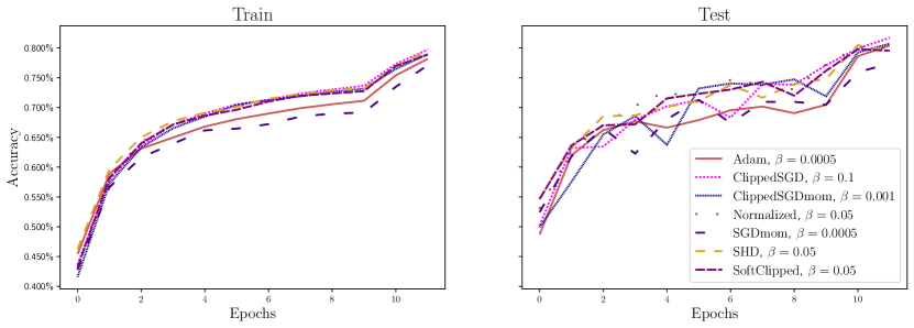
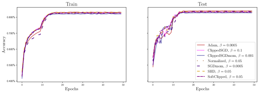
Figure 2. Accuracy of the different methods when used for training a VGG-network to classify the CIFAR10 dataset. The two plots in the top shows the first 12 epochs and the two plots in the bottom, all the 50 epochs. Each method displays the result when the optimal initial step size $\beta$ is used.

B.2.1. Details on the network architecture

The model consists of three blocks of convolutional layers. The first block consists of two convolutional layers with $32$ filters with kernel size of $3$, each followed by a batch normalization layer [Ioffe and Szegedy, 2015]. This is then passed through a max-pooling layer with a kernel size of $2\times 2$ and a stride of $2$. In the convolutional layers a weight decay of $5\cdot 10^{-3}$ is used. The next two blocks have similar structure but with filter sizes of $64$ and $128$ respectively. In between each layer a drop out of $20\%$ is used. As in the first example we use a dense hidden layer with $128$ neurons before the output layer. In all layers, the exponential linear unit was used as activation function.

B.3. Text prediction on the Pennsylvania treebank corpus

The last experiment is a long-short-term memory-type model, that we use for text prediction on the Pennsylvania Treebank portion of the Wall Street Journal corpus [Marcus et al., 1993]. The design of the experiment is inspired by similar ones in e.g. Graves [2014], Mikolov et al. [2012], Pascanu et al. [2012], Zhang et al. [2020a]. For the experiment, we use the same training and validation split of the dataset as in Merity et al. [2018].

In Figure 3 we see the exponentiated average regret, or perplexity

$$\exp\left(\frac{1}{K}\sum_{k=1}^{K}f(q_{k},\xi_{k})\right),$$

where K is the number of batches in an epoch. For a model that chooses each of the words in the vocabulary with uniform probability we expect this to be close to the size of the vocabulary (in this case $10000$). We expect a well performing model to have a perplexity close to $1$. In Figure 3, we see the training- and test perplexity for the various methods. The SHD-method achieves a slightly higher perplexity on the training data then the other methods. (Although this behavior is not as pronounced on the test data). In general, methods that make use of some sort of normalization or clipping appears to be working best for this task; the best method is the SoftClipped, which quickly reaches the lowest perplexity on the test data set.

Penn. Treebank

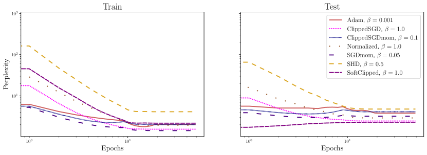
Figure 3. Perplexity of the different methods when used for text prediction on the Penn. Treebank dataset. Each method displays the result when the optimal initial step size $\beta$ is used.

B.3.1. Details on the network architecture

The network consists of an embedding layer of size $400$ upon which three bidirectional LSTM-layers are stacked, each with $1150$ RNN-units. A dropout of $50\%$ is used in the LSTM-layers, as well as weight decay of $1.2\cdot 10^{-6}$. In the output layer, a dense layer with $10000$ neurons is used. The batch size is $64$ and we use a sequence length of $10$ words.

B.4. Conclusions

The experiments in the previous section verify the theoretical results in the paper and we see that most of the algorithms also exhibit performance on par with state of the art algorithms. We remark that in all the examples, we used very generic networks for the sake of finding problems on which we could easily compare the behavior of the models. Better performance could be achieved in all cases if the networks and optimizers would have been tuned more carefully to the classification problems, but the intention here is to illustrate the behavior of the algorithms rather than achieving state of the art results.

References

- Abadi et al. (2015) M. Abadi, A. Agarwal, P. Barham, E. Brevdo, Z. Chen, C. Citro, G. S. Corrado, A. Davis, J. Dean, M. Devin, S. Ghemawat, I. Goodfellow, A. Harp, G. Irving, M. Isard, Y. Jia, R. Jozefowicz, L. Kaiser, M. Kudlur, J. Levenberg, D. Mané, R. Monga, S. Moore, D. Murray, C. Olah, M. Schuster, J. Shlens, B. Steiner, I. Sutskever, K. Talwar, P. Tucker, V. Vanhoucke, V. Vasudevan, F. Viégas, O. Vinyals, P. Warden, M. Wattenberg, M. Wicke, Y. Yu, and X. Zheng. TensorFlow: Large-scale machine learning on heterogeneous systems, 2015. URL https://www.tensorflow.org/.
- Andradóttir (1990) S. Andradóttir. A new algorithm for stochastic optimization. In O. Balci, R. Sadowski, and R. Nance, editors, Proceedings of the 1990 Winter Simulation Conference, pages 364–366, 1990.
- Asic and Adamovic (1970) M. D. Asic and D. D. Adamovic. Limit points of sequences in metric spaces. Am. Math. Mon., 77(6):613–616, 1970.
- Barakat et al. (2021) A. Barakat, P. Bianchi, W. Hachem, and S. Schechtman. Stochastic optimization with momentum: Convergence, fluctuations, and traps avoidance. Electron. J. Stat., 15(2), 2021.
- Bateman (1931) H. Bateman. On dissipative systems and related variational principles. Phys. Rev., 38, 1931.
- Bauschke and Combettes (2011) H. Bauschke and P. Combettes. Convex Analysis and Monotone Operator Theory in Hilbert Spaces. Springer, 2011.
- Beck (2017) A. Beck. First-Order Methods in Optimization. SIAM, 2017.
- Benaïm (1999) M. Benaïm. Dynamics of stochastic approximation algorithms. In J. Azéma, M. Émery, M. Ledoux, and M. Yor, editors, Séminaire de Probabilités XXXIII. Springer, 1999.
- Bengio et al. (1994) Y. Bengio, P. Simard, and P. Frasconi. Learning long-term dependencies with gradient descent is difficult. IEEE Trans. Neural Netw., 5(2), 1994.
- Bico et al. (2009) J. Bico, J. Ashmore-Chakrabarty, G. H. McKinley, and H. A. Stone. Rolling stones: The motion of a sphere down an inclined plane coated with a thin liquid film. Phys. Fluids, 21(8):082103, 2009.
- Bideau et al. (1994) D. Bideau, F. X. Riguidel, A. Hansen, G. Ristow, X. I. Wu, K. J. Måløy, and M. Ammi. Granular flow: Some experimental results. In K. K. Bardhan, B. K. Chakrabarti, and A. Hansen, editors, Non-Linearity and Breakdown in Soft Condensed Matter. Springer, 1994.
- Billingsley (1968) P. Billingsley. Convergence of Probability Measures. Wiley, 2nd edition, 1968.
- Borkar (2008) V. Borkar. Stochastic Approximation: A Dynamical Systems Viewpoint. Cambridge University Press, 2008.
- Bottou et al. (2018) L. Bottou, F. Curtis, and J. Nocedal. Optimization methods for large-scale machine learning. SIAM Rev., 60(2):223–311, 2018.
- Clevert et al. (2016) D. Clevert, T. Unterthiner, and S. Hochreiter. Fast and accurate deep network learning by exponential linear units (ELUs). In Y. Bengio and Y. LeCun, editors, 4th International Conference on Learning Representations, ICLR 2016, San Juan, Puerto Rico, May 2-4, 2016.
- Coddington and Levinson (1984) A. Coddington and N. Levinson. Theory of Ordinary Differential Equations. Krieger, 1984.
- Defazio (2021) A. Defazio. Momentum via primal averaging: Theoretical insights and learning rate schedules for non-convex optimization, 2021. arXiv: 2010.00406 [cs.LG].
- Droniou and Eymard (2016) J. Droniou and R. Eymard. Uniform-in-time convergence of numerical methods for non-linear degenerate parabolic equations. Numer. Math., 132, 2016.
- Ethier and Kurtz (1986) S. N. Ethier and T. G. Kurtz. Markov processes – characterization and convergence. Wiley, 1986.
- Fang et al. (2019) C. Fang, Z. Lin, and T. Zhang. Sharp analysis for nonconvex SGD escaping from saddle points. PMLR, 99:1192–1234, 2019.
- Fort and Pagès (1996) J.-C. Fort and G. Pagès. Convergence of stochastic algorithms: from the Kushner-Clark theorem to the Lyapounov functional method. Adv. in Appl. Probab., 28(4):1072–1094, 1996.
- Franca et al. (2020) G. Franca, J. Sulam, D. Robinson, and R. Vidal. Conformal symplectic and relativistic optimization. In H. Larochelle, M. Ranzato, R. Hadsell, M. Balcan, and H. Lin, editors, Advances in Neural Information Processing Systems, volume 33. Curran Associates, Inc., 2020.
- Franca et al. (2021) G. Franca, M. I. Jordan, and R. Vidal. On dissipative symplectic integration with applications to gradient-based optimization. J. Stat. Mech.: Theory Exp., 2021.
- Freise (2016) F. Freise. On Convergence of the Maximum Likelihood Estimator in Adaptive Designs. PhD thesis, Otto-von-Guericke-Universität Magdeburg, 2016.
- Gadat et al. (2018) S. Gadat, F. Panloup, and F. Saadane. Stochastic heavy ball. Electron. J. Stat., 12(1), 2018.
- Glendinning (1994) P. Glendinning. Stability, instability and chaos; an introduction to the theory of nonlinear differential equations. Cambridge University Press, 1994.
- Goldstein et al. (2014) H. Goldstein, C. Poole, and J. Safko. Classical Mechanics. Addison-Wesley, 3rd edition, 2014.
- Goodfellow et al. (2016) I. Goodfellow, Y. Bengio, and A. Courville. Deep Learning. MIT Press, 2016. URL http://www.deeplearningbook.org.
- Graves (2014) A. Graves. Generating sequences with recurrent neural networks, 2014. arXiv:1308.0850 [cs.NE].
- Ioffe and Szegedy (2015) S. Ioffe and C. Szegedy. Batch normalization: Accelerating deep network training by reducing internal covariate shift. In F. Bach and D. Blei, editors, Proceedings of the 32nd International Conference on Machine Learning, volume 37. PMLR, 2015.
- Jamieson and Talwalkar (2016) K. Jamieson and A. Talwalkar. Non-stochastic best arm identification and hyperparameter optimization. In A. Gretton and C. C. Robert, editors, Proceedings of the 19th International Conference on Artificial Intelligence and Statistics, volume 51, pages 240–248. PMLR, 2016.
- Kapoor and Harshvardhan (2021) J. Kapoor and Harshvardhan. A stochastic extension of Hamiltonian descent methods. Accessed 9 January 2024, 2021. URL https://harshv834.github.io/files/shd_report.pdf.
- Kingma and Ba (2015) D. Kingma and J. Ba. Adam: A method for stochastic optimization. In Y. Bengio and Y. LeCun, editors, 3rd International Conference on Learning Representations, ICLR 2015, San Diego, CA, USA, May 7-9, 2015.
- Koloskova et al. (2023) A. Koloskova, H. Hendrikx, and S. U. Stich. Revisiting gradient clipping: Stochastic bias and tight convergence guarantees. In A. Krause, E. Brunskill, K. Cho, B. Engelhardt, S. Sabato, and J. Scarlett, editors, International Conference on Machine Learning, 2023.
- Krizhevsky (2009) A. Krizhevsky. Learning multiple layers of features from tiny images. Technical report, University of Toronto, 2009.
- Kushner and Yin (2003) H. Kushner and G. Yin. Stochastic Approximation and Recursive Algorithms and Applications. Springer, 2nd edition, 2003.
- Kushner and Clark (1978) H. J. Kushner and D. S. Clark. Stochastic Approximation Methods for Constrained and Unconstrained Systems. Springer, 1st edition, 1978.
- LaSalle (1960) J. LaSalle. Some extensions of Liapunov’s second method. IRE Trans. Circuit Theory, 7(4), 1960.
- Lecun et al. (1998) Y. Lecun, L. Bottou, Y. Bengio, and P. Haffner. Gradient-based learning applied to document recognition. Proc. IEEE, 86(11):2278–2324, 1998. http://yann.lecun.com/exdb/mnist/.
- Leimkuhler and Matthews (2015) B. Leimkuhler and C. Matthews. Molecular Dynamics: With Deterministic and Stochastic Numerical Methods. Springer, 2015.
- Li et al. (2018) L. Li, K. Jamieson, G. DeSalvo, A. Rostamizadeh, and A. Talwalkar. Hyperband: A novel bandit-based approach to hyperparameter optimization. J. Mach. Learn. Res., 18, 2018.
- Livingstone et al. (2017) S. Livingstone, M. F. Faulkner, and G. Roberts. Kinetic energy choice in Hamiltonian/hybrid Monte Carlo. Biometrika, 2017.
- Ljung (1976) L. Ljung. Analysis of Recursive Stochastic Algorithms. Technical Reports TFRT-7097. Department of Automatic Control, Lund Institute of Technology (LTH), 1976.
- Maddison et al. (2018) C. J. Maddison, D. Paulin, Y. W. Teh, B. O’Donoghue, and A. Doucet. Hamiltonian descent methods, 2018. arXiv:1809.05042 [math.OC].
- Mai and Johansson (2021) V. Mai and M. Johansson. Stability and convergence of stochastic gradient clipping: Beyond Lipschitz continuity and smoothness. In M. Meila and T. Zhang, editors, Proceedings of the 38th International Conference on Machine Learning, volume 139, pages 7325–7335. PMLR, 2021.
- Marcus et al. (1993) M. P. Marcus, B. Santorini, and M. A. Marcinkiewicz. Building a large annotated corpus of English: The Penn Treebank. Comput. Linguist., 19(2):313–330, 1993.
- Merity et al. (2018) S. Merity, N. S. Keskar, and R. Socher. Regularizing and optimizing LSTM language models. In International Conference on Learning Representations, 2018.
- Mikolov (2013) T. Mikolov. Statistical language models based on neural networks. PhD thesis, Brno University of Technology, 2013.
- Mikolov et al. (2012) T. Mikolov, I. Sutskever, A. Deoras, H. Le, S. Kombrink, and J. Černocký. Subword language modeling with neural networks. Unpublished manuscript, 2012.
- Owens and Filkin (1989) A. Owens and D. L. Filkin. Efficient training of the backpropagation network by solving a system of stiff ordinary differential equations. In International 1989 Joint Conference on Neural Networks, volume 2, pages 381–386 vol.2, 1989.
- Pascanu et al. (2012) R. Pascanu, T. Mikolov, and Y. Bengio. Understanding the exploding gradient problem, 2012. arXiv:1211.5063v1 [cs.LG].
- Pascanu et al. (2013) R. Pascanu, T. Mikolov, and Y. Bengio. On the difficulty of training neural networks. In S. Dasgupta and D. McAllester, editors, Proceedings of the 30th International Conference on Machine Learning, volume 28(3), 2013.
- Paszke et al. (2019) A. Paszke, S. Gross, F. Massa, A. Lerer, J. Bradbury, G. Chanan, T. Killeen, Z. Lin, N. Gimelshein, L. Antiga, A. Desmaison, A. Kopf, E. Yang, Z. DeVito, M. Raison, A. Tejani, S. Chilamkurthy, B. Steiner, L. Fang, J. Bai, and S. Chintala. Pytorch: An imperative style, high-performance deep learning library. In H. Wallach, H. Larochelle, A. Beygelzimer, F. d'Alché-Buc, E. Fox, and R. Garnett, editors, Advances in Neural Information Processing Systems, volume 32. Curran Associates, Inc., 2019.
- Peressini et al. (1993) A. Peressini, F. Sullivan, and J. Uhl. The Mathematics of Nonlinear Programming. Springer, 1993.
- Poljak (1967) B. Poljak. A general method for solving extremum problems. Sov. Math., Dokl., 8(3), 1967.
- Polyak (1964) B. Polyak. Some methods of speeding up the convergence of iteration methods. USSR Comp. Math. Math. Phys., 4, 1964.
- Robbins and Monro (1951) H. Robbins and S. Monro. A stochastic approximation algorithm. Ann. Math. Stat., 22(3), 1951.
- Robbins and Siegmund (1971) H. Robbins and D. Siegmund. A convergence theorem for nonnegative almost supermartingales and some applications. In J. S. Rustagi, editor, Optimizing Methods in Statistics. Academic Press, 1971.
- Sebbouh et al. (2021) O. Sebbouh, R. M. Gower, and A. Defazio. Almost sure convergence rates for stochastic gradient descent and stochastic heavy ball. In M. Belkin and S. Kpotufe, editors, Proceedings of Thirty Fourth Conference on Learning Theory, volume 134. PMLR, 2021.
- Sherman (2013) J. Sherman. Nearly maximum flows in nearly linear time. In 2013 IEEE 54th Annual Symposium on Foundations of Computer Science, pages 263–269, 2013.
- Shiryaev (2016) A. Shiryaev. Probability-1. Graduate Texts in Mathematics. Springer, 3rd edition, 2016.
- Simonyan and Zisserman (2015) K. Simonyan and A. Zisserman. Very deep convolutional networks for large-scale image recognition. In International Conference on Learning Representations, 2015.
- Stoltz and Trstanova (2018) G. Stoltz and Z. Trstanova. Langevin dynamics with general kinetic energies. Multiscale Model. Sim., 16(2), 2018.
- Williams (1991) D. Williams. Probability with Martingales. Cambridge University Press, 1991.
- Wolf et al. (1998) D. Wolf, F. Radjai, and S. Dippel. Dissipation in granular materials. Philos. Mag. B, 77(5):1413–1425, 1998.
- Zeidler (1985) E. Zeidler. Nonlinear Functional Analysis and Its Applications: III: Variational Methods and Optimization. Springer, 1985.
- Zhang et al. (2020a) B. Zhang, J. Jin, C. Fang, and L. Wang. Improved analysis of clipping algorithms for non-convex optimization. In H. Larochelle, M. Ranzato, R. Hadsell, M. Balcan, and H. Lin, editors, Advances in Neural Information Processing Systems, volume 33, pages 15511–15521. Curran Associates, Inc., 2020a.
- Zhang et al. (2020b) J. Zhang, T. He, S. Sra, and A. Jadbabaie. Why gradient clipping accelerates training: A theoretical justification for adaptivity. In International Conference on Learning Representations, 2020b.