Mind the step: On the frequency-domain analysis of gravitational-wave memory waveforms

Abstract

Gravitational-wave memory is characterized by a signal component that persists after a transient signal has decayed. Treating such signals in the frequency domain is non-trivial, since discrete Fourier transforms assume periodic signals on finite time intervals. In order to reduce artifacts in the Fourier transform, it is common to use recipes that involve windowing and padding with constant values. Here we discuss how to regularize the Fourier transform in a straightforward way by splitting the signal into a given sigmoid function that can be Fourier transformed in closed form, and a residual which does depend on the details of the gravitational-wave signal and has to be Fourier transformed numerically, but does not contain a persistent component. We provide a detailed discussion of how to map between continuous and discrete Fourier transforms of signals that contain a persistent component. We apply this approach to discuss the frequency-domain phenomenology of the $(\ell=2,m=0)$ spherical harmonic mode, which contains both a memory and an oscillatory ringdown component.

I Introduction

All gravitational-wave signals observed to date are transient signals believed to originate in compact binary coalescence (CBC) Abbott et al. (2019, 2021, 2024, 2023). General relativity however predicts that such signals also contain “gravitational-wave memory”, a comparatively small component which persists after the transient has passed. Such signals thus exhibit a step-like behavior in the time domain, see for example the upper panel of Fig. 1.

Gravitational-wave memory is expected to be first observed in the next few years Lasky et al. (2016); Hübner et al. (2020); Boersma et al. (2020); Goncharov et al. (2023); Grant and Nichols (2023), and it has created great interest due to the very different character of the signal as compared with the transient component, the nonlinear nature of the effect in the merger of bound objects Blanchet and Damour (1992); Christodoulou (1991), and the connection with the Bondi-Metzner-Sachs (BMS) group of symmetries of asymptotically flat spacetimes.

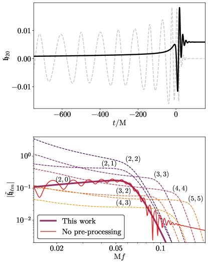
Figure 1: Spherical-harmonic decomposition of a GW signal from an aligned spin system with mass ratio 1:4 and $\chi_{1}=\chi_{2}=-0.8$ (SXS:BBH:1936). The upper panel highlights the (2,0) mode in time domain with the (rescaled) non-persistent contributions separated in gray; the lower panel displays its Fourier transform together with the other modes. The thick solid line is the frequency-domain $(2,0)$ mode after applying the pre-processing presented in this work; the thin solid line lacks any pre-processing and displays a variety of artifacts due to the finite duration of the signal.

Some of us have recently developed a computationally efficient phenomenological model of the $(\ell=2,m=0)$ spherical harmonic of quasicircular aligned spin coalescences of black holes Rosselló-Sastre et al. (2024). This mode contains the leading contribution of the gravitational-wave memory effect, as well as an oscillatory signal associated with quasi-normal ringdown, and completes the modeling of the $(\ell=2)$ modes. The model is constructed in the time domain; in GW data analysis it is however very common to work in the frequency domain, e.g. a quantity of central interest is the following scalar product Finn (1992)

$$\langle x,y\rangle=4\mathrm{Re}\int_{f_{\mathrm{min}}}^{f_{\mathrm{max}}}\mathrm{d}f\frac{\tilde{x}^{*}(f)\tilde{y}(f)}{S_{\mathrm{n}}(f)}\,,$$ (1)

where $x$ and $y$ represent two arbitrary time series, and $S_{\mathrm{n}}(f)$ is the single-sided PSD. The latter effectively sets limits on the sensitive frequency range of a detector, and thus determines which types of sources can be observed by detectors such as Advanced LIGO Aasi et al. (2015), Advanced Virgo Acernese et al. (2015), KAGRA Akutsu et al. (2019), ET Punturo et al. (2010), CE Reitze et al. (2019), or LISA Amaro-Seoane et al. (2017). In practice, the upper cutoff frequency $f_{\mathrm{max}}$ is often set by the signal, while the lower cutoff $f_{\mathrm{min}}$ is a result of the detector’s technology.

The importance of frequency-domain representations in gravitational-wave data analysis calls for an adequately simple and computationally efficient way to perform discrete Fourier transforms (FT) for step-like functions. A standard approach to carry out FTs that involve memory signals is to develop a recipe (see e.g. Gasparotto et al. (2023); Richardson et al. (2022); Chen et al. (2024)) based on windowing or padding with constant values that suppresses numerical artifacts. Here we take a different route and focus on constructing the frequency-domain version of an infinitely long signal. In order to avoid FT artifacts we simply split the signal into a sigmoid function, which can be Fourier transformed in closed form and can be chosen a priori, and a residual which does depend on the details of the gravitational-wave signal and has to be Fourier transformed numerically, but does not contain the persistent “memory” component. We then justify and provide cogent evidence for the success of our method using closed-form step-like signals and realistic GW waveforms. Note that the response of space-borne detectors such as LISA Amaro-Seoane et al. (2017), which are based on time-delay interferometry Tinto and Dhurandhar (2005), does not generate step-like data for gravitational-wave memory signals, which allows alternative avenues to process those signals, see e.g. Inchauspé et al. (2024).

As an illustration of what our method achieves, the lower panel of Fig. 1 shows the result of a straightforward numerical FT of a signal containing memory, along with the same result obtained using our method, which seamlessly suppresses numerical artifacts arising from the finite duration of the signal. To understand how our approach relates to the common recipes based on windowing, we proceed by discussing a set of examples, where for each example the behavior of the numerical FT can be reproduced in closed form. In order to facilitate the use of our method we provide a Python implementation Valencia and Tenorio (2024).

This paper is organized as follows: We first briefly review basic properties of the FT in Sec. II. In Sec. III we apply our method to a simple toy model, where FTs can be carried out in closed form. This allows us to ensure that numerical FTs reproduce the analytical results. The gravitational memory case is then treated in Sec. IV, which focuses on the FT of numerical relativity (NR) waveforms. We summarize and discuss our results in Sec. V. Finally, in Appendices A and B we discuss further details of discrete FTs.

II Fourier transforms

We define the FT to be consistent with the conventions adopted in the LIGO Algorithms Library LIGO Scientific Collaboration et al. (2018)

$$\tilde{x}(f)=\int_{-\infty}^{\infty}\mathrm{d}t\,x(t)\,e^{-i\,2\pi ft}\,.$$ (2)

For any $k$-times differentiable function $x(t)$ its FT falloff can be characterized by a power law as  Trefethen, Lloyd N. (1996)

$$\tilde{x}(f)=\mathcal{O}\left(f^{-(k+1)}\right)\,,\left|f\right|\rightarrow\infty\,$$ (3)

while smooth functions will fall off faster than any polynomial. As we will see below, in practice we will often encounter power-law falloffs, e.g. due to boundary effects when working with FTs on finite domains.

The FT of time-shifted functions $x(t-t_{0})$ gain an additional, frequency-dependent phase in the Fourier domain with respect to Eq. (2):

$$\int_{-\infty}^{\infty}\mathrm{d}t\,x(t-t_{0})\,e^{-i\,2\pi ft}=e^{-i\,2\pi ft_{0}}\tilde{x}(f)\,.$$ (4)

II.1 Fourier transforms of step-like functions

In order to prepare our treatment of the FT of step-like functions such as the memory signal shown in Fig. 1, we consider some examples where the FT can be carried out in closed form. We start with the FT of the constant function $C$, given by

$$\tilde{C}(f)=C\int_{-\infty}^{\infty}\mathrm{d}t\,e^{-i\,2\pi ft}=C\delta(f)\,.$$ (5)

An overall offset of a function thus corresponds to an $f=0$ component of the FT, usually known as the DC component. For our purposes, these effects will always be negligible, as Eq. (1) is only affected by frequencies $f>f_{\mathrm{min}}>0$.

Second, the FT of a Heaviside step function $H(t)$ reads

$$\tilde{H}(f)=\int_{0}^{\infty}\mathrm{d}t\,e^{-i\,2\pi ft}=\frac{1}{2}\delta(f)+\frac{1}{i\,2\pi f}$$ (6)

Once more we can neglect the delta and are left with a $\mathcal{O}(f^{-1})$ decay, which arises from the fact that $H(t)$ is a discontinuous function and Eq. (3).

We can construct a smooth step by using a hyperbolic tangent

$$s(t;\sigma)=\frac{1}{2}+\frac{1}{2}\mathrm{tanh}\left(\frac{t}{\sigma}\right)\,,$$ (7)

where $\sigma>0$ controls the timescale of the function’s jump. This is a regulator for the discontinuity, since this converges to $H(t)$ as $\sigma\rightarrow 0$. The corresponding FT is

$$\tilde{s}(f;\sigma) =\frac{1}{2}\delta(f)-\frac{i\pi\sigma}{2}\,\mathrm{csch}(\sigma\pi^{2}f)$$ (8)

$$=\frac{1}{2}\delta(f)-\frac{i\pi\sigma}{e^{\pi^{2}\sigma f}-e^{-\pi^{2}\sigma f}}\,.$$

As expected from Eq. (3) the high frequency behavior $\sigma f\gg 1$ is now dominated by an exponential decay

$$\left.\tilde{s}(f;\sigma)\right|_{\sigma f\gg 1}\simeq-i\,\pi\sigma e^{-\pi^{2}\sigma f}\,.$$ (9)

To leading order, the low frequency behavior $\sigma f\ll 1$ becomes

$$\left.\tilde{s}(f;\sigma)\right|_{\sigma f\ll 1}=\frac{1}{2}\delta(f)+\frac{1}{i\,2\pi f}\left[1+\mathcal{O}\left((\sigma f)^{2}\right)\right]\,.$$ (10)

which coincides with Eq. (6) as $\sigma\rightarrow 0$. Note the decay’s amplitude is independent of the step’s timescale, although the typical frequency up to which this behavior dominates does depend on $\sigma$ through $f\lesssim\sigma^{-1}$. In short, step-like features primarily affect the low-frequency Fourier components; the behavior at high frequencies, on the other hand, is governed by the smoothness of the function.

With these results we can construct a simple window function for $t\in[t_{0},t_{0}+T]$

$$w(t;t_{0},T,\sigma)=s(t-t_{0};\sigma)-s(t-t_{0}-T;\sigma)\,.$$ (11)

The FT follows from Eqs. (4) and (8) in closed form:

$$\tilde{w}(f;t_{0},T,\sigma)=e^{-i\,2\pi ft_{0}}\left(1-e^{-i\,2\pi fT}\right)\tilde{s}(f;\sigma)\,.$$ (12)

This closed-form derivation simplifies the task of analyzing the consequences of specific choices for the parameters. Since we have combined two steps separated by a certain duration and placed them at a certain initial time, Eq. (12) contains two oscillatory factors. This shows that the FTs of step-like signals with similar timescales will interfere with each other. In other words, window functions naturally introduce oscillatory artifacts in the frequency-domain signal. This will be especially relevant in Sec. III whenever GW memory is analyzed using a window, as then the expected $\mathcal{O}(f^{-1})$ falloff will gain a modulation as shown in Eq. (12).

II.2 The discrete Fourier Transform

We are interested in observational data, which will be discretely sampled at a certain frequency $f_{\mathrm{samp}}$. This causes all Fourier amplitudes at frequencies separated by a multiple of $f_{\mathrm{samp}}/2$ to fold onto each other. This phenomenon is usually known as frequency aliasing, and does not pose a problem insofar data is band-limited within the detector’s capabilities.

We represent a generic GW with a time series $\{x_{j}=x(t_{j}),j=0,\dots,N-1\}$ where each sample is labeled by a timestamp $t_{j}=t_{0}+j\delta t$. $t_{0}$ is a fiducial start time and the number of samples is given by $N=\delta tf_{\mathrm{samp}}$. The FT of this discrete dataset can then be computed as

$$\tilde{x}(f_{k}) =\int_{t_{0}}^{t_{0}+T}\mathrm{d}t\,x(t)\,e^{-i\,2\pi f_{k}t}$$ (13)

$$=e^{-i\,2\pi f_{k}t_{0}}\int_{0}^{T}\mathrm{d}t^{\prime}\,x(t^{\prime}+t_{0})\,e^{-i\,2\pi f_{k}t^{\prime}}$$ (14)

$$\approx e^{-i\,2\pi f_{k}t_{0}}\delta t\sum_{j=0}^{N-1}x_{j}e^{-i\,2\pi\frac{jk}{N}}$$ (15)

$$=e^{-i\,2\pi f_{k}t_{0}}\tilde{x}_{k}$$ (16)

where in Eq. (15) the discretisation of the continuous integral results in the discrete FT (DFT)

$$\tilde{x}_{k}=\delta t\sum_{j=0}^{N-1}x_{j}\,e^{-i\,2\pi\frac{jk}{N}}\,,$$ (17)

which can be computed efficiently using FFT algorithms Brigham and Morrow (1967).

As opposed to our original definition in Eq. (2) the integral in Eq. (13) is not symmetric; likewise, after substituting the continuous time variable by a discrete index, the index starts at 0 and an oscillatory factor corresponding to a timeshift of $t_{0}$ appears as a consequence of Eq. (4). This oscillatory behavior may become inconvenient for practical applications and can be dealt with in closed form, as discussed in Appendix A.

This correspondence between the FT and the DFT holds as long as the signals we deal with are well contained within the observing time. See Sec. III.3 for how to do it when this is not the case.

II.3 Example

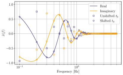
Figure 2: Comparison of discrete and continuous FT for a Gaussian function with $\mu=1.5$ and $\sigma=0.3$. The time domain grid starts at $t_{0}=-$4\text{\,}\mathrm{s}$$ and samples $N=100$ samples with a timestep of $\delta t=$0.1\text{\,}\mathrm{s}$$. DFTs are evaluated at multiples of the Rayleigh frequency $1/(\delta tN)$. Since the input signal is real, only positive frequencies are shown. The solid lines show the continuous FT [Eq. (19)]. Square markers correspond to the DFT without accounting for the shifted time origin. Circle markers show the DFT including the phase terms steming from $t_{0}\neq 0$.

To illustrate these results we use the FT of a time-shifted Gaussian function and match the continuum and discrete results. We define our Gaussian function as

$$g(t;\mu,\sigma)=\frac{1}{\sqrt{2\pi\sigma^{2}}}e^{-\frac{1}{2}\left(\frac{t-\mu}{\sigma}\right)^{2}}\,,$$ (18)

which has a corresponding continuous FT given by

$$\tilde{g}(f;\mu,\sigma)=e^{-i\,2\pi f\mu}e^{-2\pi^{2}\sigma^{2}f^{2}}$$ (19)

Note that the presence of a non-zero mean $\mu$, which shifts the function away from the origin, maps directly into a frequency oscillation as shown in Eq. (4) and discussed above.

To compute the DFT, we evaluate Eq. (18) on a discrete grid with $N=100$ points $t_{j}=t_{0}+j\delta t$ with fiducial values $t_{0}=-4$ and $\delta t=0.1$. The results are shown in Fig. 2, from which we highlight two significant features.

First, while the FT of a Gaussian on a time-symmetric interval is again real and a Gaussian, our time-shifted version, where the start and end times are not symmetric with respect to $t=0$, picks up a complex oscillation, and it is not a real function.

Second, we note the excellent agreement between the discrete (and finite) FT and the continuous Fourier transform. As previously argued, this is due to the fact that the function has died out by the time we reach the end of the domain, and thus the truncation error is identically zero at the evaluated frequencies.

III How to analyze GW memory

Before treating gravitational-wave memory signals in Sec. IV, we study a simple toy model of the (2,0) mode in the time domain and with a closed-form FT. This provides a ground truth to compare different pre-processing methods. We first discuss windowing (Sec. III.2), which has some drawbacks when dealing with step-like functions such as GW memory. To overcome those limitations we introduce Symbolic Sigmoid Subtraction SySS (Sec. III.3), which deals with the step symbolically in the time domain so artifacts are reduced. This makes it very convenient for GW memory waveforms. The code of this algorithm is publicly available as a Python package called FouTStep Valencia and Tenorio (2024).

III.1 A toy model for GW memory

The morphology of the (2,0) mode in the time domain consists of a step-like behavior ($h_{\mathrm{step}}$) that leads into an oscillatory component ($h_{\mathrm{osc}}$) at late times. These two components are described in our toy model as

$$h_{\mathrm{step}}(t;A_{\mathrm{s}},\sigma_{\mathrm{s}},t_{\mathrm{s}})=\frac{A_{\mathrm{s}}}{2}\left[1+\tanh\left(\frac{t-t_{\mathrm{s}}}{\sigma_{\mathrm{s}}}\right)\right],$$ (20)

and

$$h_{\mathrm{osc}}(t;A_{\mathrm{o}},t_{\mathrm{o}},\sigma_{\mathrm{o}},f_{\mathrm{o}})=A_{\mathrm{o}}\sin[2\pi f_{\mathrm{o}}(t-t_{\mathrm{o}})]e^{-\frac{1}{2}\left(\frac{t-t_{\mathrm{o}}}{\sigma_{\mathrm{o}}}\right)^{2}}\,,$$ (21)

where $A_{\mathrm{s},\mathrm{o}}$ are the amplitude coefficients of the step and oscillating components, $t_{\mathrm{s},\mathrm{o}}$ refer to their typical starting times, $\sigma_{\mathrm{s},\mathrm{o}}$ account for their typical timescales, and $f_{\mathrm{o}}$ refers to the oscillation’s frequency. We refer collectively to these two sets of parameters as $\lambda_{\mathrm{s}}$ and $\lambda_{\mathrm{o}}$, respectively. In the time domain the toy model then simply becomes

$$h_{\mathrm{tm}}(t;\lambda_{\mathrm{s}},\lambda_{\mathrm{o}})=h_{\mathrm{step}}(t;\lambda_{\mathrm{s}})+h_{\mathrm{osc}}(t;\lambda_{\mathrm{o}})\,.$$ (22)

The FT of both components can be expressed in closed form using the results from Sec. II:

$$\tilde{h}_{\mathrm{step}}(f;\lambda_{\mathrm{s}}) =-i\pi\sigma_{\mathrm{s}}\frac{A_{\mathrm{s}}}{2}\mathrm{csch}(\sigma_{\mathrm{s}}f\pi^{2})\,e^{-i\,2\pi ft_{\mathrm{s}}}\,,$$ (23)

$$\tilde{h}_{\mathrm{osc}}(f;\lambda_{\mathrm{o}}) =-i\sqrt{2\pi}\sigma_{\mathrm{o}}A_{\mathrm{o}}e^{-i\,2\pi ft_{\mathrm{o}}-2(\pi\sigma_{\mathrm{o}})^{2}(f^{2}+f_{\mathrm{o}}^{2})}\sinh(4\pi^{2}\sigma_{\mathrm{o}}^{2}f_{\mathrm{o}}f)\,.$$ (24)

We show an example of both the time and frequency-domain behavior of the toy model in Fig. 3. The FT displays consistent behaviors with Sec. II: The step-like contribution dominates at low frequencies, and the oscillating contribution dominates at high frequencies.

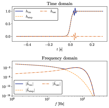
Figure 3: Representation of the GW memory toy model ($h_{\mathrm{tm}}$) together with its step ($h_{\mathrm{step}}$) and oscillatory ($h_{\mathrm{osc}}$) components in both the time (upper panel) and frequency domain (lower panel). We have used the set of parameters $A_{\mathrm{s}}=1,\,t_{\mathrm{s}}=0\,\mathrm{s},\,\sigma_{\mathrm{s}}=0.02\,\mathrm{s}$, and $A_{\mathrm{o}}=0.15,\,t_{\mathrm{o}}=0.04\,\mathrm{s},\,\sigma_{\mathrm{o}}=0.0177\,\mathrm{s},\,f_{\mathrm{o}}=66.7\,\mathrm{Hz}$. The time domain grid starts at $t_{0}=-0.5\,\mathrm{s}$ and samples $N=10^{6}$ samples with a timestep of $\delta t=8\times 10^{-6}\,\mathrm{s}$. The finite-length FTs $\tilde{h}_{\mathrm{step}}$ and $\tilde{h}_{\mathrm{osc}}$ have been computed evaluating Eqs. (23) and (24) at multiples of the Rayleigh frequency $1/(\delta tN)$. Since the time-domain input signals are real, we only show positive frequencies.

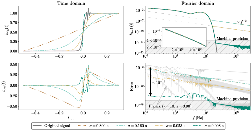
Figure 4: Comparison of different tapering functions applied to the GW memory toy model built with the same parameters as in Fig. 3. The left panel shows the resulting time-domain signal. The upper right panel shows the absolute value of the FT transform. The lower right panel shows the absolute error with respect to the closed-form result. The values of $r=0.5$ and $r=3.0$ for the Tukey and Planck windows correspond to $T=0.5\,\mathrm{s}$ and $T=1.5\,\mathrm{s}$ for the closed-form window. The number of samples of the original signal (thick black line) is $N=10^{6}$, which is increased by a factor $(1+r)$ for the windowed signals. The gray hatching approximately denotes machine precision.

Figure 5: Effect of the choice of sigmoid within the SySS approach. The sigmoids subtracted from the toy model (upper left panel) have parameters $\sigma=\{0.800\,\mathrm{s},\,0.160\,\mathrm{s},\,0.053\,\mathrm{s},\,0.008\,\mathrm{s}\}$ and $t_{\mathrm{jump}}=0\,\mathrm{s}$. The remaining residuals (lower left panel) share the same line style as their complementary sigmoid. In the frequency spectrum (upper right panel), the dashed-grey lines follow the $\mathcal{O}(f^{-2})$ decay of the FTs and the zoomed axis covers the region $f\in[1.15,5.9]\,\mathrm{Hz}$. The solid light-grey lines in the error plot (lower right panel) are the same error curves as in the lower right panel of Fig. 5, except for the Planck window with $(r=10,\varepsilon=0.90)$ pointed out with a grey arrow. In the low-frequency range, the black arrow emphasizes the difference of about 12 orders of magnitude between SySS with $\sigma=0.008\,\mathrm{s}$ and the standard windowing configurations.

III.2 Windowing

DFTs operate under the assumption that a dataset is periodic. Step-like components, as discussed in Sec. II, are interpreted as discontinuities by the DFT and give rise to accidental $\mathcal{O}(f^{-1})$ artifacts. A popular approach Gasparotto et al. (2023); Richardson et al. (2022) is to smoothly zero the data using a window function. This returns a periodic dataset, thus removing the undesired artifact. As discussed in Sec. II, however, the effect of a window function may interfere with that of the persistent memory, thus washing away the signal we were interested in the first place.

We show in Fig. 5 an example application of windowing to the memory toy model. We consider the “Tukey” Harris (1978); Tukey, J. W. (1967) and “Planck” McKechan et al. (2010) windows, which enjoy some popularity in the GW literature (see Appendix B for expressions), plus the closed-form window given in Eq. (11). We quantify the constant padding with $r$, which is the ratio between the number of padding samples and the original data samples.

At high frequencies, the windowed FT decays according to the window’s properties: the Tukey window is twice differentiable, so it decays as $\mathcal{O}(f^{-3})$, while the Planck window is smooth and decays much faster. The window defined in Eq. (11) does not reach 0 in a finite time; the data is thus not exactly periodic and the decay is $\mathcal{O}(f^{-1})$. Since for a discrete setup the computational domain is finite, these decays, based on Eq. (3), are only approximate and are cut off at $f_{\mathrm{samp}}/2$.

The error with respect to the true FT grows towards low frequencies. As discussed in Sec. II, the critical frequency up to which the window’s step behavior dominates is inversely proportional to the window’s decay timescale. Windows with timescales comparable to that of the memory, thus, return higher errors than longer windows. For the example in Fig. 5, we find that a window with three times the duration of the original signal is required to obtain an FT with an acceptable error. Incidentally, using longer windows will also increase the computing cost of this method.

III.3 Symbolic Sigmoid Subtraction

In this section we present Symbolic Sigmoid Subtraction (SySS), a simple time-domain pre-processing algorithm that subtracts a sigmoid function from the data to treat the step-like behavior symbolically. This method does not rely on any kind of windowing and has a negligible computational overhead.

The key idea is that all of the undesired artifacts shown in Fig. 1 are caused by attempting to compute the DFT of a step-like signal using a finite data stream. As discussed in Sec. II, the DFT is just an approximation to the continuous FT; thus, if the step-like behavior is subtracted in closed form, its FT can be computed in the continuum and directly added, artifact-free, to the numerical DFT of the residual signal.

In this work we choose the sigmoid function to be a hyperbolic tangent

$$h_{\mathrm{sig}}(t;A,A_{\mathrm{off}},t_{\mathrm{jump}},\sigma)=\frac{A}{2}\left[\tanh\left(\frac{t-t_{\mathrm{jump}}}{\sigma}\right)+1\right]+A_{\mathrm{off}}$$ (25)

The SySS method removes a sigmoid from the data to obtain a residual $h_{\mathrm{res}}=x-h_{\mathrm{sig}}$. The residual is free of step-like behaviors (as long as $h_{\mathrm{sig}}$ has been chosen appropriately), so $\tilde{h}_{\mathrm{res}}$ can be seamlessly computed using a DFT. The symbolic FT of $h_{\mathrm{sig}}$ (omitting DC components) is given e.g. in Eq. (23) and only needs to be multiplied by a complex phase to match the initial time $t_{0}$ of the numerical data. With this, the artifact-free FT of the data $\tilde{x}$ at a resolved frequency $f_{k}$ is given by

$$\tilde{x}(f_{k})=\tilde{h}_{\mathrm{res}\,k}+e^{i\,2\pi f_{k}t_{0}}\tilde{h}_{\mathrm{sig}}(f_{k})\,.$$ (26)

The parameters $A$ and $A_{\mathrm{off}}$ must be chosen so that $h_{\mathrm{sig}}$ matches the persistent memory offset at the ends of the dataset, and provide the additional freedom of making the average value vanish, so that $\delta$-distributions do not appear in the Fourier transform. The parameters $t_{\mathrm{jump}}$ and $\sigma$, on the other hand, should be chosen such that the “ramp up” of $h_{\mathrm{sig}}$ does not coincide with the time boundaries.

We show the results of applying SySS to the GW memory toy model in Fig. 5. The resulting frequency spectrum matches the expected result down to machine precision across the whole frequency band. In this example, this corresponds to an error reduction of up to twelve orders of magnitude with respect to windowing methods shown in Fig. 5.

The details of the behavior of SySS depends on the value chosen for $\sigma$: Low $\sigma$ produces faster transitions into the asymptotic value towards the edges of the time domain. This produces smoother residuals, which as a result tend to decay faster. If the transition is too fast, however, step-like artifacts may be accidentally introduced into the residual. These would cause again $\mathcal{O}(f^{-1})$ decays, albeit with a much lower amplitude than the original step. This can however easily be avoided. In addition, future models similar to Rosselló-Sastre et al. (2024) could just incorporate the step-function decomposition in the formulation of the model.

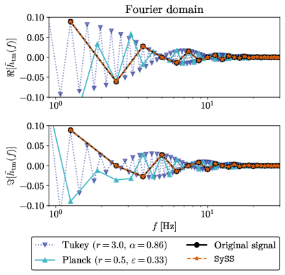
Figure 6: Low-frequency behavior of the real (upper panel) and imaginary (lower panel) part of the GW memory toy model. The analytical values (solid line + dots) are obtained from Eq. (22), while the SySS results (dashed-line + stars) correspond to the sigmoid with $\sigma=0.008\,\mathrm{s}$ in Fig. 5.

In Fig. 6 we show the real and imaginary parts of the toy model’s FT together with the results obtained using SySS and two windowing configurations. We note the excellent agreement of the SySS result. As expected, the use of windowing spreads the signal’s power into neighboring frequencies, which may cause issues with the detection and characterization of said signal Jaynes (1982); Bretthorst (1988); Allen et al. (2002); Talbot et al. (2021).

III.4 Timing comparison

The high number of likelihood evaluations required in GW data analysis makes waveform generation a computationally critical step. For time-domain waveforms, this includes the computation of the FT, as discussed in this work. We show in Fig. 7 a comparison of the computing cost of SySS versus windowing strategies. Timings are expressed as a fraction of $10\text{\,}\mathrm{ms}$, which is the average waveform evaluation time of IMRPhenomTHM using ChooseTDWaveform for an align-spin system with $\mathrm{q}=3$, $\chi_{1}=0.5$, $\chi_{2}=-0.3$ and $\mathrm{M}=100\,\mathrm{M}_{\odot}$ from $f_{\mathrm{min}}=$10\text{\,}\mathrm{Hz}$$ to $f_{\mathrm{max}}=$2048\text{\,}\mathrm{Hz}$$ with a sampling rate of $4096\text{\,}\mathrm{Hz}$ Estellés et al. (2022). This corresponds to approximately $15,000$ data points. Note that this is an illustrative example, since results will depend on the application and waveform model used.

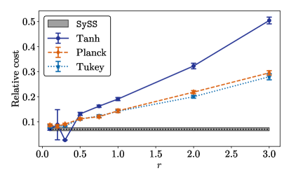
Figure 7: Computational cost of different pre-processing schemes relative to a fiducial waveform evaluation cost of 10 ms. Tanh (solid line + dot) results are obtained by computing the DFT after windowing with Eq. (11). For the Planck case (dashed line + diamond), we use our own implementation based on McKechan et al. (2010) and for the Tukey window (dotted line + star), we use the implementation in scipy Virtanen et al. (2020). The SySS method is represented with a dotted line in a shaded area. We repeat each technique 1000 times and compute the average time and standard deviation. The latter corresponds to the error bars for the windows and the height of the shaded area for SySS. All timings have been executed in a M3 Pro CPU.

The cost of windowing depends on the window’s length, which here we parametrize as the ratio $r$ between the window’s and original data’s length. Longer windows incur a higher computing cost as the FT to be computed involves a higher number of data points. SySS, on the other hand, only evaluates closed-form expressions and does not extend the duration of the dataset. Its cost is thus constant and about 7% of the evaluation time of the waveform. We remark that SySS only involves the subtraction and addition of closed-form expressions to an array with a length given by the specific application. It is thus expected that the computing cost of this method will not scale strongly with longer signals, as the only computationally-expensive operation is the computation of a closed-form expression.

As shown previously in Fig. 5, window functions must approach zero rather slowly to avoid interfering with the memory signal. In our examples, this corresponds typically to $r\gtrsim 3$. For the Tukey and Planck windows, the corresponding computing cost, shown in Fig. 7, is $\sim 30\%$ of the waveform’s evaluation time.

This comparison establishes SySS as a better approach, in the sense that it is able to return the exact FT at a smaller computing cost with no tuning required. This is because, rather than attempting to suppress a numerical artifact, SySS directly treats the root cause of the problem, namely a step-like behavior in a discrete time series, by properly treating the problem in the continuum.

IV Phenomenology of Fourier domain GW memory signals

We now turn to the treatment of actual gravitational-wave signals. The gravitational-wave strain $h$ as emitted by a binary system has two independent polarisations, $h_{+}$ and $h_{\times}$, which depend on the inertial time coordinate $t$, the distance to source $d_{\mathrm{L}}$, the intrinsic physical parameters of the source $\bm{\lambda}$, and source’s orientation angles $(\theta,\phi)$. These polarisations can be decomposed in a basis of spin-weighted spherical harmonics Goldberg et al. (1967); Wiaux et al. (2007):

$$h(t;d_{\mathrm{L}},\bm{\lambda},\theta,\phi) =h_{+}(t;d_{\mathrm{L}},\bm{\lambda},\theta,\phi)-ih_{\times}(t;d_{\mathrm{L}},\bm{\lambda},\theta,\phi)$$ (27)

$$=\frac{1}{d_{\mathrm{L}}}\sum\limits_{\ell\geq 2}\sum\limits_{|m|\leq\ell}{}^{-2}Y_{\ell m}(\theta,\phi)\,h_{\ell m}(t;\bm{\lambda})$$ (28)

where $h_{\ell m}(t;\bm{\lambda})$ are the spherical harmonic modes and depend exclusively on the time and the intrinsic physical parameters of the source. See e.g. Talbot et al. (2018) for a discussion of the spherical harmonic structure for memory waveforms.

For concreteness we focus on the $h_{20}$ spherical harmonic, which contains the dominant gravitational-wave memory contribution, however, other spherical harmonics could be treated with the same methods. The $h_{20}$ signal has two components, namely a non-oscillatory growth caused by the gravitational-wave memory effect $h_{20}^{(\text{mem})}$, and an oscillatory contribution from the quasi-normal ringdown $h_{20}^{(\text{osc})}$:

$$h_{20}(t;\bm{\lambda})=h_{20}^{(\text{mem})}(t;\bm{\lambda})+h_{20}^{(\text{osc})}(t;\bm{\lambda}).$$ (29)

The memory contribution persists after the gravitational-wave transient has passed and leaves a constant offset in the signal. This makes the amplitude to be non-zero after the merger-ringdown, which triggers artifacts in the Fourier-transformed waveform, as discussed in Sec. II. Due to this step-like morphology, SySS is a suitable pre-processing technique before computing the DFT, as we have already seen in Sec. III.

Throughout this section we fix $\theta=\pi/2$, for which the $h_{20}$-mode is maximal, and $\phi=0$. For convenience, we define

$$\mathfrak{h}_{\ell m}=(d_{\mathrm{L}}/\mathrm{M})\,^{-2}Y_{\ell m}(\theta=\pi/2,\phi=0)\,h_{\ell m}$$ (30)

and

$$\tilde{\mathfrak{h}}_{\ell m}=(d_{\mathrm{L}}/\mathrm{M}^{2})\,^{-2}Y_{\ell m}(\theta=\pi/2,\phi=0)\,\tilde{h}_{\ell m}$$ (31)

so that the time-domain (frequency-domain) strain is simply $\sum_{\ell m}\mathfrak{h}_{\ell m}$ $\left(\sum_{\ell m}\tilde{\mathfrak{h}}_{\ell m}\right)$ in geometric units.

Whenever applying SySS in this section, we choose $t_{\mathrm{jump}}$ to coincide with merger time and $\sigma=10\,\mathrm{M}$. As discussed in Sec. III.3, this choice is not unique, as SySS focuses on capturing the general step-like behavior of the signal. It is important to note that SySS is not explicitly modeling $h_{20}^{\text{(mem)}}$, but rather any step-like behavior would be successfully dealt with.

IV.1 Global picture of $h_{20}$ in the frequency domain

We start by computing the FT of a pure (2,0) NR waveform using SySS to understand the frequency-domain phenomenology of GW memory. For this, we choose an NR waveform from the SXS catalog SXS Collaboration (2019), shown in Fig. 8. As expected, the sigmoid component, which captures the step-like behavior, is dominant at low frequencies. The residual, which essentially carries the ringdown component, dominates at high frequencies.

IV.2 Memory and oscillatory contributions

In this section we apply SySS separately to $h_{20}^{\text{(mem)}}$ and $h_{20}^{\text{(osc)}}$, and we compare their frequency spectrum with the one from the most relevant higher harmonics, in different regions of the parameter space. We have computed $h_{20}^{(\mathrm{mem})}$ with Eq. (3.27) of Rosselló-Sastre et al. (2024), while $h_{20}^{\text{(osc)}}$ and the rest of the modes have been obtained directly from NR simulations of the SXS Catalog SXS Collaboration (2019).

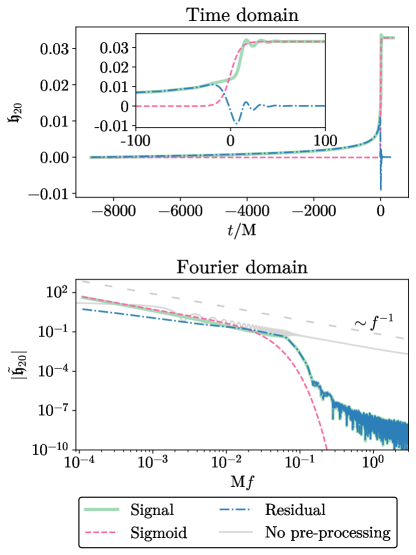
Figure 8: Time (upper panel) and Fourier (lower panel) domain of the (2,0) mode (thick solid line) for a non-spinning equal-mass binary black hole system (SXS:BBH:0001). The time range shown spans $t/\mathrm{M}\in[-8674.52,\,382.20]$. The dashed line represents the sigmoid used for SySS, while the dash-dotted line displays the residual. A closer look at the merger is shown in the zoomed axis for times between $\pm 100\,\mathrm{M}$. In the lower panel, the thin solid line represents the FT of the (2,0) mode without applying any pre-processing technique, and the loosely-dashed line shows the $\mathcal{O}(f^{-1})$ step-like decay. The memory contribution $h_{20}^{(\text{mem})}$ shown here has been computed using the sxs.waveforms.memory.add_memory option Mitman et al. (2021).

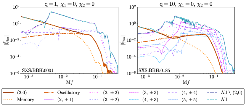
Figure 9: Frequency-domain decomposition of the GW into some of its multipolar contributions for the non-spinning systems SXS:BBH:0001 (left), and SXS:BBH:0185 (right), with mass ratios 1:1 and 1:10, respectively. The (2,0) mode (thick solid line) is split into the memory (thick dotted line) and the oscillatory (thick dash-dotted line) contributions as in Eq. (29). The memory contribution is computed from Eq. (3.27) of Rosselló-Sastre et al. (2024), while the oscillatory part and the rest of the modes are obtained from the corresponding NR simulations of the SXS Catalog SXS Collaboration (2019). The SySS method, with the standard parameters $\sigma=10\,\mathrm{M}$ and $t_{\mathrm{jump}}=t_{\mathrm{merger}}$, has been only applied to $h_{20}$, $h^{(\mathrm{mem})}_{20}$ and $h^{(\mathrm{osc})}_{20}$.

The results are shown in Figs. 9 and 10. Overall, we note differentiated behaviors between $\tilde{h}_{20}^{(\mathrm{mem})}$ and $\tilde{h}_{20}^{(\mathrm{osc})}$ for low and high frequencies, as well as a modification of the complete waveform when adding the (2,0) mode.

The memory contribution to the (2,0) mode is always dominant at low frequencies, where it behaves like a step-function with the standard $\mathcal{O}(f^{-1})$ trend. At high frequencies, however, the effect of $\tilde{h}_{20}^{(\mathrm{mem})}$ is smaller than the contribution from the oscillatory part since it has already decayed by the time the merger-ringdown takes place. This behavior is consistent with the one previously discussed in Sec. III with the toy model. Furthermore, we observe that the relative contribution of $\tilde{h}_{20}^{(\mathrm{mem})}$ to the frequency spectrum becomes larger for symmetric mass ratios and equal positive spins, which agrees with the results obtained in Rosselló-Sastre et al. (2024); Xu et al. (2024); Pollney and Reisswig (2010).

The oscillatory contribution is negligible during the inspiral, and it becomes prominent as it approaches the merger. For the non-spinning case (Fig. 9), the power coming from this contribution in the spectrum increases with the mass ratio. This behavior is also seen for spinning systems (Fig. 10). In addition, we find that $\tilde{h}_{20}^{(\mathrm{osc})}$ has a greater impact for high-negative spins, whereas it is reduced for positive spins and even more for equal positive spins, which is consistent with Rosselló-Sastre et al. (2024); Pollney and Reisswig (2010).

Including the (2,0) mode spherical harmonic in Eq. (28) always adds a $\mathcal{O}(f^{-1})$ decay at low frequencies. For larger frequencies, it can significantly modify the merger-ringdown part of the full waveform, especially for high negative spins, where the oscillatory part is louder than most of the higher harmonics (see left panels of Fig. 10).

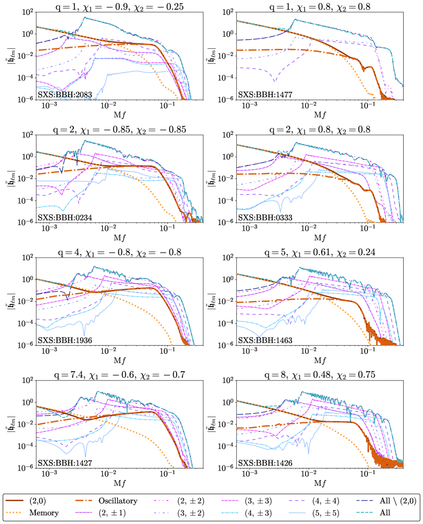
Figure 10: Same multipolar GW decomposition as in Fig. 9, but for the align-spin systems: SXS:BBH:2083, SXS:BBH:1477, SXS:BBH:0234, SXS:BBH:0333, SXS:BBH:1936, SXS:BBH:1463, SXS:BBH:1427, SXS:BBH:1426. The plots are arranged such that the left column corresponds to negative-spin systems, right column to positive-spin systems, and the mass ratio increases as one goes down a column. Furthermore, the $y$ and $x$-axes are limited to the same maximum and minimum values to facilitate comparisons between plots.

IV.3 SySS all at once

The SySS method can be applied to compute the FT of the full waveform at once. This is because we are not trying to subtract the step, but rather a step. We show an example case in Fig. 11, which demonstrates the robustness of the method. We observe a perfect agreement between two independent methods. The first one consists of computing the FT of the waveform mode by mode, where SySS is only applied to the (2,0) mode, whereas the remaining FTs are computed tapering at the early and late times. The second method, however, applies the SySS technique to the whole waveform, since it has a permanent offset originated by the contribution of the (2,0) mode.

V Discussion

GW data analysis for current ground-based detectors is typically conducted in the frequency domain. This requires a careful treatment of GW memory, which involves step-like time-domain signals and has motivated the development of multiple data-analysis recipes to suppress undesired numerical artifacts.

In this work, we presented SySS, an embarrassingly simple algorithm to treat step-like GW signals in the time domain using closed-form FTs. This new method treats step-like contributions in the continuum to avoid numerical artifacts.

We have shown the imprint that the (2,0) mode leaves in the full frequency-domain waveform. At low frequencies, it is characterized by a $\mathcal{O}(f^{-1})$ trend coming from the step component, while for high frequencies the oscillatory contribution can introduce deviations to the merger-ringdown, especially for high-negative spin systems. We found a more prominent contribution from the oscillatory part as mass ratio increases and for high-negative spin systems, whereas the memory contribution dominates for low mass ratio and positive spins. Those results are consistent with Pollney and Reisswig (2010) and the recent work done in Rosselló-Sastre et al. (2024); Xu et al. (2024).

Accuracy and timing comparisons versus windowing approaches conclude that SySS is able to match the expected FT of a step-like signal down to numerical precision at a negligible increase in computing cost. This makes SySS a particularly useful method to construct Fourier domain GW memory waveforms.

We release an open-source Python implementation of SySS Valencia and Tenorio (2024) which can be readily hooked up with the LALSuite waveform interface.

This work will help in developing future Fourier-domain models for the (2,0) mode, which can be constructed in a way that is independent of any windowing techniques. This helps in particular to develop a clear understanding of the morphology of memory signals in the frequency domain.

Appendix A Shifting in time domain

For some applications, it may be convenient to circularly time-shift the finite dataset to reduce the oscillations in the frequency domain, according to Eq. (4).

For the Gaussian example of Sec. II.3, the oscillatory behavior introduced by the phase factor of Eq. (19) can be countered by choosing a time shift $t_{\mathrm{s}}=-|t_{0}-\mu|$, which also takes into account the oscillatory component introduced by a non-zero $t_{0}$, as discussed in Sec. II.2. In general, for localized signals, $t_{\mathrm{s}}$ must be such that the dynamic range of the data is split half at the beginning of the domain and half at the end.

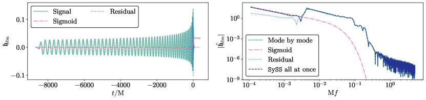
Figure 11: SySS technique applied to the GW from the equal-mass non-spinning system SXS:BBH:0001, where we have taken into account the same spherical harmonic modes shown in Figs. 9 and 10. The left panel displays the time-domain signal (thick solid line) as well as the sigmoid (dash-dotted line) and residual (dotted line) used in SySS. The parameters of the sigmoid are the same as in Fig. 9. The right panel compares the FT obtained by summing the FT of the modes one by one (thick solid line), as done in Figs. 9 and 10, with the FT obtained by applying SySS to all the modes at once (dashed line).

On the other hand, for not well-localized signals, a suitable option can be $t_{\mathrm{s}}=-|t_{0}-t_{\mathrm{max}}|$, being $t_{\mathrm{max}}$ the time where the maximum of the signal takes place.

We compare the effect of these time shifts for a Gaussian profile (Fig. 12) and a GW signal (Fig. 13). In the first case, the well location of the signal allows to remove the oscillatory components of the FT efficiently, whereas for the GW example, since there is not a well-established location, only a partial counteracting of the oscillations is achieved, mostly at high frequencies.

Appendix B Window functions

We define discrete window functions as a time series with $N$ samples labeled by $j=0,\dots,N-1$ regardless of its initial time $t_{0}$. Both of the windows here considered are parameterised by a single parameter which tunes the transition length between 0 and 1.

The Tukey window is defined as

$$w_{j} =\frac{1}{2}\left[1-\cos\left(\frac{\pi}{\Delta(\alpha)}j\right)\right] 0\leq j<\Delta(\alpha)$$ (32)

$$w_{j} =1 \Delta(\alpha)\leq j\leq(N-1)/2$$ (33)

$$w_{j} =w_{(N-1)-j} (N-1)/2<j\leq N-1$$ (34)

where $\Delta(\alpha)=\alpha(N-1)/2$ is the transition interval and we assume integer division. This window is only twice differentiable.

The Planck window is defined as

$$w_{j} =0 j=0$$ (35)

$$w_{j} =\left[1+e^{\left(\frac{\Delta(\varepsilon)}{j}-\frac{\Delta(\varepsilon)}{\Delta(\varepsilon)-j}\right)}\right]^{-1} 1\leq j<\Delta(\varepsilon)$$ (36)

$$w_{j} =1 \Delta(\varepsilon)\leq j\leq(N-1)/2$$ (37)

$$w_{j} =w_{(N-1)-j} (N-1)/2<j\leq N-1$$ (38)

where $\Delta(\varepsilon)=\varepsilon(N-1)$. This window is based on a bump function, which is smooth.

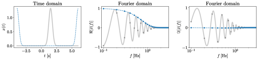
Figure 12: Effect of a time shift in the FT of a Gaussian with parameters $\mu=1.5\,\mathrm{s}$ and $\sigma=0.3\,\mathrm{s}$. The left panel shows the time-domain unshifted Gaussian profile (thick solid line) and the same profile after a time shift of $t_{\mathrm{s}}=-|t_{0}-\mu|$ (dashed line). The time grid starts at $t_{0}=-4\,\mathrm{s}$ and samples $N=500$ points with a constant time step $\delta t=0.02\,\mathrm{s}$. The middle and right panels represent the real and imaginary parts of the continuous (lines) and discrete (markers) FTs. The discrete version has been evaluated at multiples of the Rayleigh frequency $1/(N\delta t)$.

Figure 13: Same as in Fig. 12 but for a GW signal for a non-spinning equal-mass system. The waveform has been generated with the LALSuite software infrastructure using the approximant IMRPhenomTHM Estellés et al. (2022) including only the (2,2) mode. Without loss of generality, we have aligned the waveform at the peak so that $t_{\mathrm{max}}=0$. Unlike in Fig. 12, no continuous FT is displayed here.

References

- Abbott et al. (2019) B.P. Abbott et al. (LIGO Scientific, Virgo), “GWTC-1: A Gravitational-Wave Transient Catalog of Compact Binary Mergers Observed by LIGO and Virgo during the First and Second Observing Runs,” Phys. Rev. X 9, 031040 (2019), arXiv:1811.12907 [astro-ph.HE] .
- Abbott et al. (2021) R. Abbott et al. (LIGO Scientific, Virgo), “GWTC-2: Compact Binary Coalescences Observed by LIGO and Virgo During the First Half of the Third Observing Run,” Phys. Rev. X 11, 021053 (2021), arXiv:2010.14527 [gr-qc] .
- Abbott et al. (2024) R. Abbott et al. (LIGO Scientific, VIRGO), “GWTC-2.1: Deep extended catalog of compact binary coalescences observed by LIGO and Virgo during the first half of the third observing run,” Phys. Rev. D 109, 022001 (2024), arXiv:2108.01045 [gr-qc] .
- Abbott et al. (2023) R. Abbott et al. (KAGRA, LIGO Scientific, VIRGO), “GWTC-3: Compact Binary Coalescences Observed by LIGO and Virgo during the Second Part of the Third Observing Run,” Phys. Rev. X 13, 041039 (2023), arXiv:2111.03606 [gr-qc] .
- Lasky et al. (2016) Paul D. Lasky et al., “Detecting gravitational-wave memory with LIGO: implications of GW150914,” Phys. Rev. Lett. 117, 061102 (2016), arXiv:1605.01415 [astro-ph.HE] .
- Hübner et al. (2020) Moritz Hübner, Colm Talbot, Paul D. Lasky, and Eric Thrane, “Measuring gravitational-wave memory in the first LIGO/Virgo gravitational-wave transient catalog,” Phys. Rev. D 101, 023011 (2020), arXiv:1911.12496 [astro-ph.HE] .
- Boersma et al. (2020) Oliver M. Boersma, David A. Nichols, and Patricia Schmidt, “Forecasts for detecting the gravitational-wave memory effect with Advanced LIGO and Virgo,” Phys. Rev. D 101, 083026 (2020), arXiv:2002.01821 [astro-ph.HE] .
- Goncharov et al. (2023) Boris Goncharov, Laura Donnay, and Jan Harms, “Inferring fundamental spacetime symmetries with gravitational-wave memory: from LISA to the Einstein Telescope,” arXiv e-prints (2023), arXiv:2310.10718 [gr-qc] .
- Grant and Nichols (2023) Alexander M. Grant and David A. Nichols, “Outlook for detecting the gravitational-wave displacement and spin memory effects with current and future gravitational-wave detectors,” Phys. Rev. D 107, 064056 (2023), [Erratum: Phys.Rev.D 108, 029901 (2023)], arXiv:2210.16266 [gr-qc] .
- Blanchet and Damour (1992) Luc Blanchet and Thibault Damour, “Hereditary effects in gravitational radiation,” Phys. Rev. D 46, 4304–4319 (1992).
- Christodoulou (1991) Demetrios Christodoulou, “Nonlinear nature of gravitation and gravitational-wave experiments,” Phys. Rev. Lett. 67, 1486–1489 (1991).
- Rosselló-Sastre et al. (2024) Maria Rosselló-Sastre, Sascha Husa, and Sayantani Bera, “A waveform model for the missing quadrupole mode from black hole coalescence: memory effect and ringdown of the spherical harmonic,” arXiv e-prints (2024), arXiv:2405.17302 [gr-qc] .
- Finn (1992) Lee S. Finn, “Detection, measurement and gravitational radiation,” Phys. Rev. D 46, 5236–5249 (1992), arXiv:gr-qc/9209010 .
- Aasi et al. (2015) J. Aasi et al. (LIGO Scientific), “Advanced LIGO,” Class. Quant. Grav. 32, 074001 (2015), arXiv:1411.4547 [gr-qc] .
- Acernese et al. (2015) F. Acernese et al. (VIRGO), “Advanced Virgo: a second-generation interferometric gravitational wave detector,” Class. Quant. Grav. 32, 024001 (2015), arXiv:1408.3978 [gr-qc] .
- Akutsu et al. (2019) T. Akutsu et al. (KAGRA), “KAGRA: 2.5 Generation Interferometric Gravitational Wave Detector,” Nature Astron. 3, 35–40 (2019), arXiv:1811.08079 [gr-qc] .
- Punturo et al. (2010) M. Punturo et al., “The Einstein Telescope: A third-generation gravitational wave observatory,” Class. Quant. Grav. 27, 194002 (2010).
- Reitze et al. (2019) David Reitze et al., “Cosmic Explorer: The U.S. Contribution to Gravitational-Wave Astronomy beyond LIGO,” Bull. Am. Astron. Soc. 51, 035 (2019), arXiv:1907.04833 [astro-ph.IM] .
- Amaro-Seoane et al. (2017) Pau Amaro-Seoane et al., “Laser Interferometer Space Antenna,” arXiv e-prints (2017), arXiv:1702.00786 [astro-ph.IM] .
- Gasparotto et al. (2023) Silvia Gasparotto et al., “Can gravitational-wave memory help constrain binary black-hole parameters? a lisa case study,” Phys. Rev. D 107 (2023), 10.1103/physrevd.107.124033.
- Richardson et al. (2022) Colter J. Richardson et al., “Modeling core-collapse supernovae gravitational-wave memory in laser interferometric data,” Phys. Rev. D 105 (2022), 10.1103/physrevd.105.103008.
- Chen et al. (2024) Yitian Chen et al., “Improved frequency spectra of gravitational waves with memory in a binary-black-hole simulation,” arXiv e-prints (2024), arXiv:2405.06197 [gr-qc] .
- Tinto and Dhurandhar (2005) Massimo Tinto and Sanjeev V. Dhurandhar, “TIME DELAY,” Living Rev. Rel. 8, 4 (2005), arXiv:gr-qc/0409034 .
- Inchauspé et al. (2024) Henri Inchauspé et al., “Measuring gravitational wave memory with LISA,” arXiv e-prints (2024), arXiv:2406.09228 [gr-qc] .
- Valencia and Tenorio (2024) Jorge Valencia and Rodrigo Tenorio, “gw-foutstep,” https://github.com/valencia-jorge/gw-foutstep (2024).
- LIGO Scientific Collaboration et al. (2018) LIGO Scientific Collaboration, Virgo Collaboration, and KAGRA Collaboration, “LVK Algorithm Library - LALSuite,” Free software (GPL) (2018).
- Trefethen, Lloyd N. (1996) Trefethen, Lloyd N., “Finite difference and spectral methods for ordinary and partial differential equations,” Unpublished text, http://people.maths.ox.ac.uk/trefethen/pdetext.html (1996).
- Brigham and Morrow (1967) E. O. Brigham and R. E. Morrow, “The fast fourier transform,” IEEE Spectr. 4, 63–70 (1967).
- Harris (1978) F.J. Harris, “On the use of windows for harmonic analysis with the discrete fourier transform,” Proc. IEEE 66, 51–83 (1978).
- Tukey, J. W. (1967) Tukey, J. W., “An introduction to the calculations of numerical spectrum analysis,” In Bernard Harris, editor, Spectral analysis of time series, pages 25–46. Wiley (1967).
- McKechan et al. (2010) D. J. A. McKechan, C. Robinson, and B. S. Sathyaprakash, “A tapering window for time-domain templates and simulated signals in the detection of gravitational waves from coalescing compact binaries,” Class. Quant. Grav. 27, 084020 (2010), arXiv:1003.2939 [gr-qc] .
- Jaynes (1982) Edwin T. Jaynes, “On the rationale of maximum-entropy methods,” Proceedings of the IEEE 70, 939–952 (1982).
- Bretthorst (1988) G Larry Bretthorst, Bayesian spectrum Analysis and parameter estimation (Springer-Verlag Berlin Heidelberg, 1988).
- Allen et al. (2002) Bruce Allen, Maria Alessandra Papa, and Bernard F. Schutz, “Optimal strategies for sinusoidal signal detection,” Phys. Rev. D 66, 102003 (2002), arXiv:gr-qc/0206032 .
- Talbot et al. (2021) Colm Talbot, Eric Thrane, Sylvia Biscoveanu, and Rory Smith, “Inference with finite time series: Observing the gravitational Universe through windows,” Phys. Rev. Res. 3, 043049 (2021), arXiv:2106.13785 [astro-ph.IM] .
- Estellés et al. (2022) Héctor Estellés et al., “Time-domain phenomenological model of gravitational-wave subdominant harmonics for quasicircular nonprecessing binary black hole coalescences,” Phys. Rev. D 105, 084039 (2022), arXiv:2012.11923 [gr-qc] .
- Virtanen et al. (2020) Pauli Virtanen et al., “SciPy 1.0: Fundamental Algorithms for Scientific Computing in Python,” Nature Methods 17, 261–272 (2020).
- Goldberg et al. (1967) J. N. Goldberg et al., “Spin-s Spherical Harmonics and ð,” J. Math. Phys. 8, 2155–2161 (1967), https://pubs.aip.org/aip/jmp/article-pdf/8/11/2155/19109311/2155_1_online.pdf .
- Wiaux et al. (2007) Y. Wiaux, L. Jacques, and P. Vandergheynst, “Fast spin ±2 spherical harmonics transforms and application in cosmology,” J. Comput. Phys. 226, 2359–2371 (2007).
- Talbot et al. (2018) Colm Talbot, Eric Thrane, Paul D. Lasky, and Fuhui Lin, “Gravitational-wave memory: waveforms and phenomenology,” Phys. Rev. D 98, 064031 (2018), arXiv:1807.00990 [astro-ph.HE] .
- SXS Collaboration (2019) SXS Collaboration, “SXS Gravitational Waveform Database,” https://www.black-holes.org/waveforms (2019).
- Mitman et al. (2021) K. Mitman et al., “Adding gravitational memory to waveform catalogs using bms balance laws,” Phys. Rev. D 103, 024031 (2021).
- Xu et al. (2024) Yumeng Xu et al., “Enhancing Gravitational Wave Parameter Estimation with Non-Linear Memory: Breaking the Distance-Inclination Degeneracy,” arXiv e-prints (2024), arXiv:2403.00441 [gr-qc] .
- Pollney and Reisswig (2010) Denis Pollney and Christian Reisswig, “Gravitational memory in binary black hole mergers,” Astrophys. J. 732, L13 (2010).