A Random Integration Algorithm for High-dimensional Function Spaces

Liang Chen,  Minqiang Xu Haizhang Zhang Department of Mathematics, Jiujiang University, Jiujiang, 332000, P. R. China. E-mail address: chenliang3@mail2.sysu.edu.cn.Corresponding Author. College of Science, Zhejiang University of Technology, Hangzhou, 310023, P. R. China. E-mail address: mqxu@zjut.edu.cn. Supported in part by National Natural Science Foundation of China (No. 12326346, 12326347), and by Zhejiang Provincial Natural Science Foundation of China (No. ZCLY24A0101).School of Mathematics (Zhuhai), Sun Yat-sen University, Zhuhai, 519082, P. R. China. E-mail address: zhhaizh2@sysu.edu.cn. Supported in part by National Natural Science Foundation of China under grant 12371103, and by Guangdong Basic and Applied Basic Research Foundation (2024A1515011194).
Abstract

We introduce a novel random integration algorithm that boasts both high convergence order and polynomial tractability for functions characterized by sparse frequencies or rapidly decaying Fourier coefficients. Specifically, for integration in periodic isotropic Sobolev space and the isotropic Sobolev space with compact support, our approach attains a nearly optimal root mean square error (RMSE) bound. In contrast to previous nearly optimal algorithms, our method exhibits polynomial tractability, ensuring that the number of samples does not scale exponentially with increasing dimensions. Our integration algorithm also enjoys nearly optimal bound for weighted Korobov space. Furthermore, the algorithm can be applied without the need for prior knowledge of weights, distinguishing it from the component-by-component algorithm. For integration in the Wiener algebra, the sample complexity of our algorithm is independent of the decay rate of Fourier coefficients. The effectiveness of the integration is confirmed through numerical experiments.

Keywords: Numerical integration; Monte Carlo; Curse of dimensionality; Sample complexity

MSC 2020: 65D30, 68Q25, 65C05, 42B10

1 Introduction

This paper is concerned with numerically integrating multivariate functions defined over the $d$-dimensional unit cube. Denote

$$\operatorname{INT}(f):=\int_{[0,1]^{d}}f(x)dx.$$

Evaluating $\operatorname{INT}(f)$ amounts to estimating the value of $\hat{f}(0)$, wherein the Fourier transform is defined as

$$\hat{f}(w)=\int_{[0,1]^{d}}f(x)\exp(-2\pi iw\cdot x)dx.$$ (1)

For a given positive integer $N$, we introduce the following discrete Fourier transform

$$\widetilde{f}^{(N)}(w)=\frac{1}{N^{d}}\sum_{t\in\{\frac{z}{N}|z\in\mathbb{Z}_{N}^{d}\}}f(x)\exp(-2\pi iw\cdot t),\quad w\in\mathbb{Z}^{d}$$

where $\mathbb{Z}_{N}^{d}:=\mathbb{Z}^{d}\cap[0,N)^{d}$.

Inspired by the sparse Fourier transform (SFT) from signal processing [2, 13, 20], our approach to estimating $\hat{f}(0)$ involves two key steps. First, we create a hash map that effectively disperses the frequencies, ensuring that the energy of frequencies near zero (excluding zero itself) is small. Second, we employ a low-pass filter to extract the low-frequency components. Here, we utilize the hash mapping $A_{N}$ developed in our previous paper [2],

$$A_{N}:=\begin{pmatrix}\mathbf{I}_{d-1}&{\bf 0}\\ {\boldsymbol{v}}&h_{d}\end{pmatrix},$$ (2)

where $N$ is some prime number, $\mathbf{I}_{d-1}$ represents the identity matrix of order $d-1$, ${\boldsymbol{v}}:=(h_{1},h_{2},\dots,h_{d-1})$, and $({\boldsymbol{v}},h_{d})$ is drawn from the uniform distribution on the set $\mathbb{Z}^{d}\cap[1,N)^{d}$. Note that the distribution here differs from the setting in [2]. Subsequently, we construct the following low-pass filter:

$$f_{A_{N},L,r}(x):=\sum_{|l|\leq L}f(\{A_{N}^{\top}(x-y_{l})\})G_{L,r,l},$$ (3)

where $\{t\}\in[0,1)$ denotes the fractional part of $t$ (for instance, $\{3.2\}=0.2$, $\{-1.3\}=0.7$), $y_{l}=(0,\dots,0,l/N)^{\top}$, and

$$G_{L,r,l}=\sum_{{|l+kN|\leq L,k\in\mathbb{Z}}}\frac{1}{r\sqrt{2\pi}}\exp(-\frac{(l+kN)^{2}}{2r^{2}}).$$

The function $G_{L,r,l}$ can be conceptualized as a truncated periodic Gaussian window, inspired by the Sinc-Gauss window described in [20]. The comprehensive attributes of $G_{L,r,l}$ are elaborated in Lemma 2.2. By letting $z=A_{N}^{\top}x$ and substituting it into Eq.(3), we derive the following critical integration formula

$$I(f)_{H_{N},L,r,z}:=\sum_{|l|\leq L}f\bigg{(}\bigg{\{}\frac{z-lH_{N}}{N}\bigg{\}}\bigg{)}G_{L,r,l},$$ (4)

where $H_{N}$ and $z$ are drawn from the uniform distribution over $\mathbb{Z}^{d}\cap[1,N)^{d}$ and $\mathbb{Z}^{d}\cap[0,N)^{d}$, respectively.

When employing other recent high-dimensional SFT methods for estimating numerical integration, as cited in references [23, 25, 19], it is not feasible to achieve the desired error bounds for functions in Sobolev spaces. Previously, Gilbert et.al [13] introduced an algorithmic framework for high-dimensional SFT, which could potentially be adapted to develop integration algorithms that attain the desired error bound. However, such a framework would increase the upper bound by a factor of $d^{5}$, as analyzed on page 61 of [25]. In addition, Eq.Β (4) can also be viewed as a special random lattice rule. Recently, a series of studies [28, 9, 30, 32, 16] have explored the use of random lattice rules for estimating numerical integration in weighted Korobov spaces, drawing inspiration from the pioneering contributions of Bakhvalov [1].

Utilizing Eq.Β (4), along with the local Monte Carlo sampling (see Eq.(7)) and the median trick [24, 31, 29, 17, 33, 34, 18], we shall construct a novel randomized integration algorithm. The contributions of this paper are outlined as follows:

  • β€’

    Our random algorithm is nearly optimal for integration in the periodic isotropic Sobolev space as well as in the isotropic Sobolev space with compact support, while maintaining polynomial tractability. Consequently, it is also nearly optimal and polynomially tractable for smooth functions that vanish on the boundary. In contrast, previous works [27, 35] have developed optimal integration algorithms for the mixed Sobolev space and the isotropic Sobolev space with compact support. However, these algorithms suffer from a drawback: their RMSE upper bounds involve constants larger than $2^{\Theta(d)}$ (where $d$ denotes the dimension, see Remark 3.2 in [35]. Specifically, in [27], the corresponding constant is larger than $1/(d^{d/2}(2^{1/d}-1)^{d})$ and the order of the Sobolev space is required to be greater than $d/2$, as observed from the proofs of Theorem 1 and Lemma 5 in [27]), rendering them not polynomially tractable in terms of sample complexity. More recently, [5] proposes a nearly optimal integration algorithm for general smooth functions and smooth functions that vanish on the boundary of $[0,1]^{d}$ (see Theorem 3.2 in [5]). However, as acknowledged in the β€œFuture work” section of [5], they still struggle to overcome the curse of dimensionality in terms of sample complexity.

  • β€’

    Our constructive algorithm is also nearly optimal for integration in weighted Korobov space. Unlike the algorithms [28, 9, 30, 32, 16], our algorithm does not require prior information about weights, making it universally applicable to varying weights in the RMSE sense. The integration algorithms applicable to different weights under the worst-case scenario have been established in [12, 6, 8, 11, 17].

  • β€’

    Our algorithm achieves a convergence rate of order $\frac{\log^{\Theta(1)}(n)}{n}$ (where $n$ denotes the sample size) for integration in the Wiener algebra. In comparison to previous studies conducted under the worst-case scenario [7, 10, 14, 15, 3, 26], our random algorithm converges at a faster rate. Notably, the sample complexity of our algorithm is independent of the decay rate of Fourier coefficients and the HΓΆlder continuity of the functions, provided that we choose a sufficiently large $N$ in Eq. (4).

The outline of this paper is structured as follows: In Section 2, we provide a theoretical analysis of the algorithm. Section 3 further explores this analysis. Subsequently, in Section 4, we present numerical experiments to validate the effectiveness of the algorithm.

2 Integration in Isotropic Sobolev Spaces and the Wiener Algebra

We start with some technical lemmas. For two nonnegative functions $h,g$ on a common domain, we shall write $h(\tau)=\Theta(g(\tau))$ if there exist absolute constants $C_{1},C_{2}>0$ such that $C_{1}g(\tau)<h(\tau)<C_{2}g(\tau)$ for every $\tau$ in the domain. Also denote by $\mathbb{I}_{U}(\cdot)$ and $\#U$ the indicator function and the cardinality of $U$, respectively. In this paper, all hidden constants are absolute constants.

We define the median of a set of complex numbers $\{a_{j}\}_{j=1}^{k}$ as $median\{a_{j}\}_{j=1}^{k}=median\{\Re a_{j}\}_{j=1}^{k}+i\times median\{\Im a_{j}\}_{j=1}^{k}$, where $median\{\Re a_{j}\}_{j=1}^{k}$ and $median\{\Im a_{j}\}_{j=1}^{k}$ represent the median of the real part and the imaginary part of $\{a_{j}\}_{j=1}^{k}$, respectively. According to Proposition 1 in [29], we have the following corollary.

Lemma 2.1.

Let $\mathcal{W}$ be a given function space with semi-norm $\|\cdot\|_{\mathcal{W}}$. If $R_{m}$ is a random algorithm such that

$$\sup_{\|f\|_{\mathcal{W}}\leq 1}\mathbb{P}\left\{\left|R_{m}(f)-\operatorname{INT}(f)\right|>\epsilon\right\}\leq\alpha,$$

where $0<\epsilon,\alpha<1/2$, then for an odd positive integer $k$, it holds

$$\sup_{\|f\|_{\mathcal{W}}\leq 1}\mathbb{P}\left\{\left|median\{R_{m,j}(f)\}_{j=1}^{k}-\operatorname{INT}(f)\right|>2\epsilon\right\}\leq 2^{k}\alpha^{k/2},$$

where $\{R_{m,j}(f)\}_{j=1}^{k}$ is a set of $k$ independent realizations of $R_{m}(f)$.

Lemma 2.2.

Let $0<\epsilon<1/2$ and $L,r,N$ be such that $1<B<r<L<N/2$, where $r=\Theta(B\sqrt{\log(1/\epsilon)})$, $L=r\sqrt{2\log(1/\epsilon)}$. Then it holds

$$\biggl{|}1-\sum_{|l|\leq L}G_{L,r,l}\biggr{|}\leq\Theta(\epsilon),$$

and

$$\sum_{|l|\leq L}G_{L,r,l}\exp(2\pi iwl/N)\leq\Theta(\epsilon)~{}\text{for~{}any ~{}}w\notin[-\frac{N}{B},\frac{N}{B}]\,({\rm mod}N).$$
Proof.

Let

$$G_{r,l}=\sum_{k\in\mathbb{Z}}\frac{1}{r\sqrt{2\pi}}\exp(-\frac{(l+kN)^{2}}{2r^{2}}).$$

Based on Claim 7.2 in [20] (see the full version: arXiv:1201.2501v2), we have

$$\sum_{l\in\mathbb{Z}_{N}}G_{r,l}\exp(2\pi iwl/N)=\sum_{k\in\mathbb{Z}}\exp(-2(\pi r(k+w/N))^{2}).$$

Given that $N>2L$ and $L=r\sqrt{2\log(1/\epsilon)}$, utilizing Lemma 2.6 in [4], we obtain

$$|G_{L,r,l}-G_{r,l}|\leq\Theta\bigg{(}\frac{\epsilon}{r\sqrt{2\pi}}\exp(-\frac{l^{2}}{2r^{2}})\bigg{)}\quad\text{for}\quad l\in[-L,L]\,({\rm mod}N),$$

and

$$\sum_{l\in\mathbb{Z}_{N}\backslash([0,L]\cup[N-L,N-1])}G_{r,l}\leq\Theta(\epsilon).$$

Therefore,

$$\biggl{|}\sum_{|l|\leq L}G_{L,r,l}\exp(2\pi iwl/N)-\sum_{l\in\mathbb{Z}_{N}}G_{r,l}\exp(2\pi iwl/N)\biggr{|}\leq\Theta(\epsilon).$$ (5)

Since $r=\Theta(B\sqrt{\log(1/\epsilon)})$, we conclude that

$$\biggl{|}\sum_{l\in\mathbb{Z}_{N}}G_{r,l}\exp(2\pi iwl/N)\biggr{|}\leq\Theta(\epsilon)\quad\text{for}\quad w\notin\bigg{[}-\frac{N}{B},\frac{N}{B}\bigg{]}({\rm mod}N).$$ (6)

Combining Eq. (5) and (6) verifies Lemma 2.2. This completes the proof. ∎

The lemma presented below closely resembles Lemma 3.2 in [2] and Lemma 4 in [28].

We shall write $\xi\sim\mbox{unif}\,\Omega$ to mean that $\xi$ is a random variable having the uniform distribution on the set $\Omega$, and write $\xi_{1},\xi_{2},\cdots,\xi_{m}\stackrel{{\scriptstyle iid}}{{\sim}}\operatorname{unif}\,\Omega$ to mean that $\xi_{1},\xi_{2},\cdots,\xi_{m}$ are drawn i.i.d. from the uniform distribution on $\Omega$.

Lemma 2.3.

Let $N$ be a prime number and $B>0$. Then, for any $w\in\mathbb{Z}^{d}$ with wβ‰ 0​(mod​N)𝑀0mod𝑁w\neq 0\,({\rm mod}N), it holds

$$H_{N}\cdot w\in[-N/B,N/B]\,({\rm mod}N),$$

with probability at most $\Theta(1/B)$ over the randomness of $H_{N}$, where $H_{N}:=(h_{1},h_{2},\dots,h_{d})\stackrel{{\scriptstyle iid}}{{\sim}}\operatorname{unif}\,\mathbb{Z}^{d}\cap[1,N)^{d}.$

Proof.

Since wβ‰ 0​(mod​N)𝑀0mod𝑁w\neq 0\,({\rm mod}N), there must be a component whose absolute value is not less than $1$. Without loss of generality, let us assume that the $d$-th component $w_{d}$ satisfies wdβ‰ 0​(mod​N)subscript𝑀𝑑0mod𝑁w_{d}\neq 0\,({\rm mod}N). Then, fixing arbitrary values $h_{1},\dots,h_{d-1}$, with probability at most $\Theta(1/B)$(no greater than the ratio of the length of the interval $[-N/B,N/B]$ to $\Theta(N)$) over the randomness of $h_{d}$, we have

$$\sum_{i=1}^{d}h_{i}w_{i}\in[-N/B,N/B]\,({\rm mod}N),$$

thereby completing the proof. ∎

For any function $f:[0,1]^{d}\rightarrow\mathbb{C}$, we introduce a new function $f_{N,\eta}$ defined as

$$f_{N,\eta}(z/N):=f(z/N+\eta_{z}),$$ (7)

where $z\in\mathbb{Z}_{N}^{d}$, and $\eta_{z}\sim\operatorname{unif}\,[0,1/N)^{d}$.

Lemma 2.4.

Let $f$ be a function of the form

$$f(x)=a_{0}+g(x)+R(x),\quad x\in[0,1]^{d},$$

where $\|f\|_{L^{2}([0,1]^{d})}\leq 1$, $\operatorname{INT}(R)=0$, and

$$g(x)=\sum_{\xi\in U}a_{\xi}\exp(2\pi i\xi\cdot x)$$

with $U\subset\mathbb{Z}^{d}\cap(-\mathcal{M},\mathcal{M})^{d}\backslash\{0\}$. Choosing $K=\#U$ and $N=\Theta(\sqrt{d}K\mathcal{M}/\epsilon)$, with probability at least $1-1/10-\frac{1}{\epsilon^{2}N^{d}}$ over the randomness of $\eta$, we have

$$f_{N,\eta}(z/N)=a_{0}^{*}+g(z/N)+R_{2}(z/N),$$

where $|a_{0}^{*}-a_{0}|\leq\Theta(\epsilon)$, $\operatorname{INT}(R_{2})=0$, and

$$\frac{1}{N^{d}}\sum_{z\in\mathbb{Z}_{N}^{d}}|R_{2}(z/N)|^{2}\leq 20\|R\|_{L^{2}([0,1]^{d})}^{2}+\Theta(\epsilon^{2}).$$
Proof.

Since $\mathbb{E}_{\eta}\widetilde{f}_{N,\eta}^{(N)}(0)=a_{0}$, and $\mathbb{E}_{\eta}|\widetilde{f}_{N,\eta}^{(N)}(0)-a_{0}|^{2}\leq\frac{1}{N^{d}}$, by Chebyshev’s inequality,

$$|\widetilde{g}_{N,\eta}^{(N)}(0)+\widetilde{R}_{N,\eta}^{(N)}(0)|=|\widetilde{f}_{N,\eta}^{(N)}(0)-a_{0}|\leq\epsilon$$

with probability at least $1-\frac{1}{\epsilon^{2}N^{d}}$ over the randomness of $\eta$.

Notice

$$\mathbb{E}_{\eta}\frac{1}{N^{d}}\sum_{z\in\mathbb{Z}_{N}^{d}}|R_{N,\eta}(z/N)|^{2}=\|R\|_{L^{2}([0,1]^{d})}^{2}.$$

By Markov’s inequality, with probability at least $1-1/10$, it holds

$$\frac{1}{N^{d}}\sum_{z\in\mathbb{Z}_{N}^{d}}|R_{N,\eta}(z/N)|^{2}\leq 10\|R\|_{L^{2}([0,1]^{d})}^{2}.$$

Finally, observe that

$$|g_{N,\eta}(z/N)-g(z/N)|=\biggl{|}\sum_{\xi\in U}(a_{\xi}\exp(2\pi i\xi\cdot\eta_{z})-a_{\xi})\exp(2\pi i\xi\cdot z/N)\biggr{|}\leq\Theta(K\sqrt{d}\mathcal{M}/N)\leq\Theta(\epsilon).$$

Letting

$$R_{2}(z/N):=R_{N,\eta}(z/N)+g_{N,\eta}(z/N)-g(z/N)-\widetilde{g}_{N,\eta}^{(N)}(0)-\widetilde{R}_{N,\eta}^{(N)}(0)$$

finishes the proof. ∎

To establish the theoretical analysis of our algorithm, we meticulously define the function space as follows:

$$\begin{split}&F_{K,\mathcal{M},\lambda_{1},\lambda_{2}}:=\bigg{\{}f(x)=a_{0}+\bigg{(}\sum_{j=1}^{K}a_{j}\exp(2\pi iw^{(j)}\cdot x)\bigg{)}+R(x)\\ &\bigg{|}w^{(j)}\in\mathbb{Z}^{d}\cap(-\mathcal{M},\mathcal{M})^{d}\backslash\{0\},\,\sum_{j\geq 1}|a_{j}|\leq\lambda_{1},\operatorname{INT}(R)=0,\|R\|_{L^{2}([0,1]^{d})}^{2}\leq\lambda_{2}\bigg{\}}.\end{split}$$ (8)

It is clear from the definition that $\operatorname{INT}(f)=a_{0}$ for any $f\in F_{K,\mathcal{M},\lambda_{1},\lambda_{2}}$.

Theorem 2.5.

Let $1/100<\sigma<1/10$, $0<\epsilon<\sigma$, $B=\Theta(K/\sigma)$, $r=\Theta(B\sqrt{\log(1/\epsilon)})$, $L=r\sqrt{2\log(1/\epsilon)}$, and $N=\Theta(\max\{1/(\sqrt{\sigma}\epsilon)^{2/d}),\sqrt{d}K\mathcal{M}/\epsilon\})$ be a prime number. For each $f\in F_{K,\mathcal{M},\lambda_{1},\lambda_{2}}$ with $\|f\|_{L^{2}([0,1]^{d})}\leq 1$, $\lambda_{1},\lambda_{2}\geq 1$,it holds with probability at least $1-\sigma-1/10$ over the randomness of $H_{N}$, $z$ and $\eta$ that

$$\big{|}I(f_{N,\eta})_{H_{N},L,r,z}-\operatorname{INT}(f)\big{|}\leq\Theta(\lambda_{1}\epsilon+\sqrt{\lambda_{2}/K}),$$ (9)

provided that $1<B<r<L<N/2$, and $\epsilon<\sigma/K$.

Taking the median of outputs $\{I(f_{N,\eta})_{H_{N_{j}},L,r,z_{j}}\}_{j=1}^{t}$, which are obtained by independently randomizing $H_{N}$, $z$ and $\eta$ for $t$ times with $t\geq 7$ being an odd integer, we have the following holds with probability at least $1-(2\sqrt{\sigma+1/10})^{t}$

$$\big{|}median\{I(f_{N,\eta_{j}})_{H_{N_{j}},L,r,z_{j}}\}_{j=1}^{t}-\operatorname{INT}(f)\big{|}\leq\Theta(\lambda_{1}\epsilon+\sqrt{\lambda_{2}/K}).$$ (10)

Furthermore, the RMSE of the integration method is bounded by

$$\begin{split}&\bigg{(}\mathbb{E}_{\{H_{N_{j}},z_{j},\eta_{j}\}_{j=1}^{t}}\big{|}median\{I(f_{N,\eta_{j}})_{H_{N_{j}},L,r,z_{j}}\}_{j=1}^{t}-\operatorname{INT}(f)\big{|}^{2}\bigg{)}^{1/2}\\ &\leq\Theta\bigg{(}\lambda_{1}+\sqrt{\lambda_{2}/K}+(2\sqrt{\sigma+1/10})^{t}\bigg{)}.~{}~{}~{}~{}~{}~{}~{}~{}~{}~{}~{}~{}~{}~{}\end{split}$$ (11)
Proof.

A function $f\in F_{K,\mathcal{M},\lambda_{1},\lambda_{2}}$ can be expressed as

$$f(x)=a_{0}+\bigg{(}\sum_{j=1}^{K}a_{j}\exp(2\pi iw^{(j)}\cdot x)\bigg{)}+R(x),$$ (12)

with the conditions

$$\sum_{j\geq 1}|a_{j}|\leq\lambda_{1},\operatorname{INT}(R)=0,~{}\text{and}~{}\|R\|_{L^{2}([0,1]^{d})}^{2}\leq\lambda_{2}.$$

For brevity, we denote the second term on the right side of Eq.(12) as $g$. Then $f$ can be rewritten as

$$f(x)=a_{0}+g(x)+R(x).$$

By choosing a prime number $N=\Theta(\max\{1/(\sqrt{\sigma}\epsilon)^{2/d}),\sqrt{d}K\mathcal{M}/\epsilon\})$ and using Lemma 2.4, with probability at least $1-\sigma-1/10$, we have

$$f_{N,\eta}(z/N)=a_{0}^{*}+g(z/N)+R_{2}(z/N),\quad z\in\mathbb{Z}_{N}^{d},$$ (13)

where $|a_{0}^{*}-a_{0}|\leq\Theta(\epsilon)$ and $\frac{1}{N^{d}}\sum_{z\in\mathbb{Z}_{N}^{d}}|R_{2}(z/N)|^{2}\leq 20\|R\|_{L^{2}([0,1]^{d})}^{2}+\Theta(\epsilon^{2}).$ Suppose

$$R_{2}(z/N)=\sum_{\xi\in\mathbb{Z}_{N}^{d}\backslash\{0\}}c_{\xi}\exp(2\pi i\xi\cdot z/N).$$

Then $\sum_{z\in\mathbb{Z}_{N}^{d}}|c_{\xi}|^{2}\leq 20\lambda_{3}+\Theta(\epsilon^{2})$.

We will analyze the last two terms on the right side of Eq. (13) separately. Let $B=\Theta(K/\sigma)$, $r=\Theta(B\sqrt{\log(N/\epsilon)})$, and $L=r\sqrt{2\log(N/\epsilon)}$. By Lemma 2.3,

$$H_{N}\cdot w^{(j)}\in\bigg{[}-\frac{N}{B},\frac{N}{B}\bigg{]}({\rm mod}N),1\leq j\leq K$$

holds with probability at most $\sigma/K$. Therefore, we have,

$$\mathbb{P}\bigg{\{}H_{N}\cdot w^{(j)}\in\bigg{[}-\frac{N}{B},\frac{N}{B}\bigg{]}({\rm mod}N)~{}\text{holds}~{}\text{for}~{}\text{every}~{}j=1,2,\dots,K\bigg{\}}\geq 1-\sigma.$$

Furthermore, by Lemma 2.2,

$$\mathbb{P}\bigg{\{}\sum_{|l|\leq L}g_{1}\bigg{(}\bigg{\{}\frac{z-lH_{N}}{N}\bigg{\}}\bigg{)}G_{L,r,l}\leq\lambda_{1}\epsilon~{}\text{holds}~{}\text{for}~{}\text{every}~{}z\in\mathbb{Z}_{N}^{d}\bigg{\}}\geq 1-\sigma.$$ (14)

Next, we analyze $R_{2}$. For each $\xi\in\mathbb{Z}_{N}^{d}\backslash\{0\}$, denote

$$t_{\xi}:=\frac{1}{N^{d}}\sum_{z\in[0,N)^{d}}\bigg{|}\sum_{|l|\leq L}c_{\xi}\exp\bigg{(}2\pi i\xi\cdot\bigg{\{}\frac{z-lH_{N}}{N}\bigg{\}}\bigg{)}G_{L,r,l}\bigg{|}^{2},$$

and

$$U_{H_{N},B}:=\biggl{\{}\xi|H_{N}\cdot\xi\in\big{[}-\frac{N}{B},\frac{N}{B}\big{]}({\rm mod}N)\biggr{\}}.$$

Then the combination of Lemma 2.2 and Lemma 2.3 yields

$$\begin{split}\mathbb{E}_{H_{N}}t_{\xi}&=\mathbb{E}_{H_{N}}\big{(}t_{\xi}|\xi\in U_{H_{N},B}\big{)}\mathbb{P}\left\{\xi\in U_{H_{N},B}\right\}+\mathbb{E}_{H_{N}}\big{(}t_{\xi}|\xi\notin U_{H_{N},B}\big{)}\mathbb{P}\left\{\xi\notin U_{H_{N},B}\right\}\\ &\leq\Theta\bigg{(}\frac{|c_{\xi}|^{2}}{B}+\epsilon^{2}|c_{\xi}|^{2}\bigg{)},\end{split}$$

where $H_{N}{\sim}\operatorname{unif}\,Z^{d}\cap[1,N)^{d}$. Note that for every distinct $\xi,\eta\in\mathbb{Z}_{N}^{d}$,

$$\sum_{z\in\mathbb{Z}_{N}^{d}}\bigg{(}\sum_{|l|\leq L}\exp\bigg{(}2\pi i\xi\cdot\bigg{\{}\frac{z-lH_{N}}{N}\bigg{\}}\bigg{)}G_{L,r,l}\bigg{)}\bigg{(}\sum_{|l|\leq L}\exp\bigg{(}2\pi i\eta\cdot\bigg{\{}\frac{z-lH_{N}}{N}\bigg{\}}\bigg{)}G_{L,r,l}\bigg{)}=0.$$ (15)

Therefore,

$$\mathbb{E}_{H_{N}}\mathbb{E}_{z}\bigg{|}\sum_{|l|\leq L}R_{2}\bigg{(}\bigg{\{}\frac{z-lH_{N}}{N}\bigg{\}}\bigg{)}G_{L,r,l}\bigg{|}^{2}=\mathbb{E}_{H_{N}}\sum_{\xi\in\mathbb{Z}^{d}\cap[0,N]^{d}\backslash\{0\}}t_{\xi}\leq\Theta\bigg{(}\frac{\lambda_{2}}{B}+(\lambda_{2}+1)\epsilon^{2}\bigg{)},$$ (16)

where $z\sim\mbox{unif}\ \mathbb{Z}_{N}^{d}$. Recalling the condition $\epsilon<\sigma/K$, we obtain the following inequality by applying Markov’s inequality,

$$\mathbb{P}\bigg{\{}\bigg{|}\sum_{|l|\leq L}R_{2}\bigg{(}\bigg{\{}\frac{z-lH_{N}}{N}\bigg{\}}\bigg{)}G_{L,r,l}\bigg{|}^{2}\leq\Theta\bigg{(}\frac{\lambda_{2}}{K}\bigg{)}\bigg{\}}\geq 1-\sigma.$$ (17)

Summarizing Eqs. (13, 14, 17), and applying Markov’s Inequality, we obtain

$$\mathbb{P}\bigg{\{}\bigg{|}\sum_{|l|\leq L}f\bigg{(}\bigg{\{}\frac{z-lH_{N}}{N}\bigg{\}}\bigg{)}G_{L,r,l}-a_{0}\bigg{|}\leq\Theta(\lambda_{1}\epsilon+\sqrt{\lambda_{2}/K})\bigg{\}}\geq 1-3\sigma-1/10.$$

By randomly selecting $H_{N}$, $z$ and $\eta$ to compute $I(f_{N,\eta})_{H_{N},L,r,z}$ $t$ times, we obtain $t$ different results. Extracting the median of the obtained results, the estimation (10) can be naturally derived from Lemma 2.1. Denote the median by $Y$. Then

$$\begin{split}&~{}~{}~{}~{}\mathbb{E}_{\{H_{N_{j}},z_{j},\eta_{j}\}_{j=1}^{t}}\big{|}median\{I(f_{N,\eta_{j}})_{H_{N_{j}},L,r,z_{j}}\}_{j=1}^{t}-\operatorname{INT}(f)\big{|}^{2}\\ &\leq\sum_{k\geq 0}\mathbb{P}\{200k\leq|Y|\leq 200(k+1)\}\mathbb{E}_{\{H_{N_{j}},z_{j},\eta_{j}\}_{j=1}^{t}}\bigg{(}\big{|}Y-\operatorname{INT}(f)\big{|}^{2}\bigg{|}200k\leq|Y|\leq 200(k+1)\bigg{)}\\ &=:\sum_{k\geq 0}E_{k}.\end{split}$$ (18)

Combining $|\operatorname{INT}(f)|\leq 1$ and Eq. (10), we obtain that

$$E_{0}\leq\bigg{(}\Theta(\lambda_{1}\epsilon+\sqrt{\lambda_{3}/K}+\lambda_{2}/K)+201(2\sqrt{\sigma+1/10})^{t}\bigg{)}^{2}.$$

Notice

$$\mathbb{E}_{\eta}\mathbb{E}_{z}|I(f_{N,\eta})_{H_{N},L,r,z}|\leq\bigg{(}\sum_{|l|\leq L}G_{L,r,l}\bigg{)}\mathbb{E}_{\eta}\mathbb{E}_{z}|f_{N,\eta}(z/N)|\leq 2\|f\|_{L^{2}([0,1]^{d})}\leq 2,$$

Thus, for $k\geq 1$, it holds that

$$\mathbb{P}\{|I(f_{N,\eta})_{H_{N},L,r,z}|\geq 200k\}\leq\frac{1}{100k},$$

and

$$\mathbb{P}\{|Y|\geq 200k\}\leq\binom{t}{\frac{t+1}{2}}\bigg{(}\frac{1}{100k}\bigg{)}^{\frac{t+1}{2}}\leq(2/\sqrt{100})^{t}/k^{\frac{t+1}{2}}.$$

Therefore,

$$E_{k}\leq(200(k+2))^{2}(2/\sqrt{100})^{t}/k^{\frac{t+1}{2}},\quad\text{for}\quad k\geq 1.$$

Given that $t\geq 7$, there exists an absolute constant $C$ such that

$$\sum_{k\geq 1}(k+2)^{2}/k^{\frac{t+1}{2}}\leq C.$$

Consequently,

$$\sum_{k\geq 1}E_{k}\leq\Theta((2/\sqrt{100})^{t}),$$

and

$$\begin{split}&~{}~{}~{}~{}\bigg{(}\mathbb{E}_{\{H_{N_{j}},z_{j},\eta_{j}\}_{j=1}^{t}}\big{|}median\{I(f_{N,\eta})_{H_{N_{j}},L,r,z_{j}}\}_{j=1}^{t}-\operatorname{INT}(f)\big{|}^{2}\bigg{)}^{1/2}\\ &\leq(\sum_{k\geq 0}E_{k})^{1/2}\leq\Theta(\lambda_{1}\epsilon+\sqrt{\lambda_{3}/K}+\lambda_{2}/K+(2\sqrt{\sigma+1/10})^{t}).\end{split}$$ (19)

This completes the proof. ∎

We are now in position to formulate an accurate estimation for the unit ball of periodic isotropic Sobolev space

$$H^{s}(\mathcal{T}^{d}):=\left\{f\in L^{2}(\mathcal{T}^{d})\bigg{|}\|f\|_{H^{s}(\mathcal{T}^{d}))}^{2}:=\sum_{w=(w_{1},\dots,w_{d})\in\mathbb{Z}^{d}}(1+(\sum_{j=1}^{d}|2\pi w_{j}|)^{s})^{2}|\hat{f}(w)|^{2}\leq 1\right\},$$

where $\mathcal{T}=\mathbb{R}/\mathbb{Z}=[0,1)$.

Theorem 2.6.

Let $f\in H^{s}(\mathcal{T}^{d})$ with $s\geq 0$. Given $1/100<\sigma<1/10$ and $0<\epsilon<\sigma$, let $N=\Theta(\max\{1/(\sqrt{\sigma}\epsilon)^{2/d}),\sqrt{d}B^{1+1/d}/\epsilon\})$ be a prime number, $n>0$, $B=\Theta(n/\sigma)$, $r=\Theta(B\sqrt{\log(1/\epsilon)}/)$, $L=r\sqrt{2\log(1/\epsilon)}$, and assume $B<r<L<N/2$ and $\epsilon<\sigma/n$. It holds with probability at least $1-\sigma-1/10$ over the randomness of $H_{N}$, $z$ and $\eta$ that

$$\bigg{|}I(f_{N,\eta})_{H_{N},L,r,z}-\operatorname{INT}(f)\bigg{|}\leq\Theta\bigg{(}\frac{1}{n^{s/d+1/2}}+n\epsilon\bigg{)}.$$ (20)

By obtaining the $median\{I(f_{N,\eta_{j}})_{H_{N_{j}},L,r,z_{j}}\}_{j=1}^{t}$ as in Theorem 2.5, we have the following holds with probability at least $1-(2\sqrt{\sigma+1/10})^{t}$,

$$\big{|}median\{I(f_{N,\eta_{j}})_{H_{N_{j}},L,r,z_{j}}\}_{j=1}^{t}-\operatorname{INT}(f)\big{|}\leq\Theta\bigg{(}\frac{1}{n^{s/d+1/2}}+n\epsilon\bigg{)}.$$ (21)

Furthermore, the RMSE is bounded by

$$\begin{split}\bigg{(}\mathbb{E}_{\{H_{N_{j}},z_{j},\eta_{j}\}_{j=1}^{t}}\big{|}median\{I(f_{N,\eta})_{H_{N_{j}},L,r,z_{j}}\}_{j=1}^{t}-\operatorname{INT}(f)\big{|}^{2}\bigg{)}^{1/2}\\ \leq\Theta\bigg{(}\frac{1}{n^{s/d+1/2}}+n\epsilon+(2\sqrt{\sigma+1/10})^{t}\bigg{)}.~{}~{}~{}~{}~{}~{}~{}~{}~{}~{}~{}~{}~{}~{}~{}~{}\end{split}$$ (22)
Proof.

Let $n$ be a positive number, and define $\beta_{n,d}=\frac{n^{1/d}}{2\pi}$. For any $f\in H^{s}(\mathcal{T}^{d})$, we decompose $f$ into the following form:

$$f(x)=a_{0}+g(x)+R(x),$$

where

$$g(x)=\sum_{w\in\mathbb{Z}^{d}\cap(-\beta_{n,d},\beta_{n,d})^{d}\backslash\{0\}}a_{w}\exp(2\pi iw\cdot x),$$

and

$$R(x)=\sum_{w\notin\mathbb{Z}^{d}\cap(-\beta_{n,d},\beta_{n,d})^{d}}a_{w}\exp(2\pi iw\cdot x).$$

Since $f\in H^{s}(\mathcal{T}^{d})$, we have $\|R\|_{L^{2}([0,1]^{d})}\leq\Theta(n^{-\frac{s}{d}}\|f\|_{L^{2}([0,1]^{d})})$ and

$$\#\{w|w\in\mathbb{Z}^{d}\cap(-\beta_{n,d},\beta_{n,d})^{d}\backslash\{0\}\}\leq n.$$

Let $N=\Theta(1/(\sqrt{\sigma}\epsilon)^{2/d}))$ and $B=\Theta(n/\sigma)$. Theorem 2.6 follows directly from Theorem 2.5. ∎

Given a bounded measurable set $\Omega$ with volume $1$, we denote the unit ball of the isotropic Sobolev spaces with compact support over $\Omega$ by H̊s​(Ξ©)superscriptΜŠπ»π‘ Ξ©\mathring{H}^{s}(\Omega). Here the assumption $|\Omega|=1$ aligns with the specifications outlined in [35]. For any f∈H̊s​(Ξ©)𝑓superscriptΜŠπ»π‘ Ξ©f\in\mathring{H}^{s}(\Omega), we can define

$$F(x)=\sum_{k\in\mathbb{Z}^{d}}f(k+x).$$

It is noteworthy that

$$\int_{\Omega}f(x)dx=\int_{\mathcal{T}^{d}}F(x)dx\quad\text{and}\quad\|F\|_{H^{s}(\mathcal{T}^{d})}\leq 1.$$

Thus the error bounds (20), (21), and (22) stated previously remain valid for $\operatorname{INT}(F)=\int_{\Omega}f(x)dx$. A pertinent question arises regarding the number of samples required to determine the value of $F(x)$. More precisely, based on Eq. (4), how many samples are necessary to obtain the values of the set $\big{\{}F_{N,\eta}\big{(}\big{\{}\frac{z-lH_{N}}{N}\big{\}}\big{)}\big{\}}_{l=-L}^{L}$? Let us define

$$\mathbb{J}^{\Omega}(x):=\sum_{k\in\mathbb{Z}^{d}}\mathbb{I}_{\Omega}(k+x),$$

where $\mathbb{I}_{\Omega}$ is the indicator function of $\Omega$. With a certain probability, we only require $\Theta(L)$ samples. In fact,

$$\begin{split}2L+1=(2L+1)\mbox{volume}(\Omega)=(2L+1)\int_{\Omega}\mathbb{I}_{\Omega}(x)dx~{}~{}~{}~{}~{}~{}~{}~{}~{}~{}~{}~{}~{}~{}~{}~{}~{}~{}~{}~{}~{}~{}~{}~{}~{}~{}~{}~{}~{}~{}~{}~{}~{}~{}~{}~{}~{}~{}~{}\\ =(2L+1)\int_{[0,1]^{d}}\mathbb{J}^{\Omega}(x)dx=\sum_{l=-L}^{L}\mathbb{E}_{\eta_{l}}\mathbb{E}_{z}\mathbb{J}_{N,\eta_{l}}^{\Omega}(\frac{z-lH_{N}}{N})~{}~{}~{}~{}~{}~{}~{}~{}~{}~{}~{}~{}~{}~{}~{}~{}~{}~{}~{}~{}~{}~{}~{}~{}~{}~{}~{}~{}~{}\\ =\mathbb{E}_{\eta_{1}}\mathbb{E}_{\eta_{2}}\cdots\mathbb{E}_{\eta_{l}}\mathbb{E}_{z}\sum_{l=-L}^{L}\#\{z-lH_{N}+\eta_{l}+k\big{|}k\in\mathbb{Z}^{d},z-lH_{N}+\eta_{l}+k\in\Omega\},\end{split}$$

where $z{\sim}\operatorname{unif}\mathbb{Z}^{d}\cap[0,N)^{d}$ and $\{\eta_{l}\}_{l=-L}^{L}\stackrel{{\scriptstyle iid}}{{\sim}}\operatorname{unif}\,[0,1/N)^{d}$. Then by Markov’s inequality,

$$\mathbb{P}\left\{\sum_{l=-L}^{L}\#\{z-lH_{N}+\eta_{l}+k\big{|}k\in\mathbb{Z}^{d},z-lH_{N}+\eta_{l}+k\in\Omega\}\geq 200L+100\right\}\leq 1/100.$$

In other words, with a probability of at least $99/100$, the number of samples required to obtain $\bigg{\{}F_{N,\eta}\big{(}\big{\{}\frac{z-lH_{N}}{N}\big{\}}\big{)}\biggl{\}}_{l=-L}^{L}$ is at most $200L+100$.

When searching the sets

$$V_{l}:=\{z-lH_{N}+\eta_{l}+k\big{|}k\in\mathbb{Z}^{d},z-lH_{N}+\eta_{l}+k\in\Omega\},-L\leq l\leq L,$$

we do not require any samples of the function $f$. Upon discovering that the number of elements in the union $\cup_{-L\leq l\leq L}V_{l}$ exceeds $200L+100$, we promptly output the result (denoted as $I^{*}(F_{N,\eta})_{H_{N},L,r,z}$) as zero. Otherwise, we set $I^{*}(F_{N,\eta})_{H_{N},L,r,z}=I(F_{N,\eta})_{H_{N},L,r,z}$. Therefore, for the function $F$, the probability of success for Eq. (20), where $f$ is replaced with $F$, with a required sample size of at most $200L+100$ is $1-\sigma-1/10-1/100$. This ensures that the sample complexity of our algorithm remains polynomial with respect to $d$. Consequently, we have the following corollary.

Corollary 2.7.

Let f∈H̊s​(Ξ©)𝑓superscriptΜŠπ»π‘ Ξ©f\in\mathring{H}^{s}(\Omega) and define $F(x)=\sum_{k\in\mathbb{Z}^{d}}f(k+x)$. Assume the same parameter settings as those in Theorem 2.6. Then it holds with probability at least $1-\sigma-1/10-1/100$ over the randomness of $H_{N}$, $z$ and $\eta$ that

$$\bigg{|}I^{*}(F_{N,\eta})_{H_{N},L,r,z}-\operatorname{INT}(F)\bigg{|}\leq\Theta\bigg{(}\frac{1}{n^{s/d+1/2}}+n\epsilon\bigg{)}.$$

By obtaining the $median\{I^{*}(F_{N,\eta_{j}})_{H_{N_{j}},L,r,z_{j}}\}_{j=1}^{t}$ as in Theorem 2.5, we have the following holds with probability at least $1-(2\sqrt{\sigma+1/10+1/100})^{t}$,

$$\big{|}median\{I^{*}(F_{N,\eta_{j}})_{H_{N_{j}},L,r,z_{j}}\}_{j=1}^{t}-\operatorname{INT}(F)\big{|}\leq\Theta\bigg{(}\frac{1}{n^{s/d+1/2}}+n\epsilon\bigg{)}.$$

Furthermore, the RMSE is bounded by

$$\begin{split}\bigg{(}\mathbb{E}_{\{H_{N_{j}},z_{j},\eta_{j}\}_{j=1}^{t}}\big{|}median\{I^{*}(F_{N,\eta})_{H_{N_{j}},L,r,z_{j}}\}_{j=1}^{t}-\operatorname{INT}(F)\big{|}^{2}\bigg{)}^{1/2}\\ \leq\Theta\bigg{(}\frac{1}{n^{s/d+1/2}}+n\epsilon+(2\sqrt{\sigma+1/10+1/100})^{t}\bigg{)}.~{}~{}~{}~{}~{}~{}~{}~{}~{}~{}~{}~{}~{}~{}~{}~{}\end{split}$$
Remark 2.8.

We define the isotropic Sobolev space in accordance with the definition provided in [35], albeit with minor variations from the one presented in [27]. Nevertheless, the conclusion remains valid for the isotropic Sobolev space with compact support defined in [27].

We further deduce the subsequent theorem pertaining to the Wiener algebra, which is defined as follows:

$$\mathcal{A}(\mathcal{T}^{d}):=\left\{f\in C(\mathcal{T}^{d})\Bigg{|}\|f\|_{\mathcal{A}}:=\sum_{\boldsymbol{k}\in\mathbb{Z}^{d}}|\hat{f}(\boldsymbol{k})|<\infty\right\}.$$
Theorem 2.9.

Let $f\in\mathcal{A}(\mathcal{T}^{d})$ with $\|f\|_{\mathcal{A}}\leq 1$. Let $0<\epsilon<1/2$, $1/100<\sigma<1/10$, $n>0$, $B=\Theta(n/\sigma)$, $r=\Theta(B\sqrt{\log(1/\epsilon)}/)$, $L=r\sqrt{2\log(1/\epsilon)}$. Also let $N=\Theta(1/(\sqrt{\sigma}\epsilon)^{2/d})$ be a prime number and assume $B<r<L<N/2$, $\epsilon<\sigma/n$. Then it holds with probability at least $1-\sigma-1/10$ over the randomness of $H_{N}$, $z$ and $\eta$ that

$$\bigg{|}I(f_{N,\eta})_{H_{N},L,r,z}-\operatorname{INT}(f)\bigg{|}\leq\Theta\bigg{(}\frac{1}{n}+\epsilon+\sum_{w\in\mathbb{Z}^{d}\backslash[-N\epsilon/\sqrt{d},N\epsilon/\sqrt{d}]^{d}}|\hat{f}(w)|\bigg{)}.$$ (23)

With $median\{I(f_{N,\eta_{j}})_{H_{N_{j}},L,r,z_{j}}\}_{j=1}^{t}$ as in Theorem 2.5, it holds with probability at least $1-(2\sqrt{\sigma+1/10})^{t}$ that

$$\big{|}median\{I(f_{N,\eta_{j}})_{H_{N_{j}},L,r,z_{j}}\}_{j=1}^{t}-\operatorname{INT}(f)\big{|}\leq\Theta\bigg{(}\frac{1}{n}+\epsilon+\sum_{\mathbb{Z}^{d}\backslash[-N\epsilon/\sqrt{d},N\epsilon/\sqrt{d}]^{d}}|\hat{f}(w)|\bigg{)}.$$ (24)

Furthermore,

$$\begin{split}\bigg{(}\mathbb{E}_{\{H_{N_{j}},z_{j},\eta_{j}\}_{j=1}^{t}}\big{|}median\{I(f_{N,\eta})_{H_{N_{j}},L,r,z_{j}}\}_{j=1}^{t}-\operatorname{INT}(f)\big{|}^{2}\bigg{)}^{1/2}\\ \leq\Theta\bigg{(}\frac{1}{n}+\epsilon+\sum_{\mathbb{Z}^{d}\backslash[-N\epsilon/\sqrt{d},N\epsilon/\sqrt{d}]^{d}}|\hat{f}(w)|+(2\sqrt{\sigma+1/10})^{t}\bigg{)}.\end{split}$$ (25)
Proof.

Let $f(x):=\sum a_{w}\exp(2\pi iw\cdot x),$ where $\sum|a_{w}|\leq 1$. Following a similar approach as in the proof of Lemma 2.4, we establish that

$$|~{}f_{N,\eta}^{(N)}(0)-a_{0}|\leq\epsilon$$

holds with probability at least $1-\frac{1}{\epsilon^{2}N^{d}}$ over the randomness of $\eta$. Let

$$g(z/N):=\sum_{w\in\mathbb{Z}^{d}\cap[-N\epsilon/\sqrt{d},N\epsilon/\sqrt{d}]^{d}\backslash\{0\}}a_{w}\exp(2\pi iw\cdot z/N).$$

Observe that

$$|g_{N,\eta}(z/N)-g(z/N)|\leq\sum_{w\in\mathbb{Z}^{d}\cap[-N\epsilon/\sqrt{d},N\epsilon/\sqrt{d}]^{d}}|a_{w}\exp(2\pi iw\cdot\eta_{z})-a_{w}|\leq\Theta(\epsilon).$$

We decompose $f_{N,\eta}$ as

$$f_{N,\eta}(z/N)=a_{0}^{*}+g(z/N)+R(z/N),$$ (26)

where $|a_{0}^{*}-a_{0}|\leq\epsilon$, and

$$\|R\|_{L^{\infty}([0,1]^{d})}\leq\Theta(\epsilon)+\sum_{\mathbb{Z}^{d}\backslash[-N\epsilon/\sqrt{d},N\epsilon/\sqrt{d}]^{d}}|\hat{f}(w)|.$$

Let $U_{H_{N},B}:=\{w|H_{N}\cdot w\in\big{[}-\frac{N}{B},\frac{N}{B}\big{]}({\rm mod}N)\}.$ By combining the results of Lemmas 2.2 and Lemma 2.3, we obtain

$$\begin{split}\mathbb{E}_{H_{N}}\bigg{|}\sum_{|l|\leq L}g\bigg{(}\bigg{\{}\frac{z-lH_{N}}{N}\bigg{\}}\bigg{)}G_{L,r,l}\bigg{|}\leq\sum_{w\in\mathbb{Z}_{N}^{d}\backslash\{0\}}\mathbb{E}_{H_{N}}|a_{w}|\bigg{|}\sum_{|l|\leq L}\exp(2\pi iw\cdot(z-lH_{N})/N)G_{L,r,l}\bigg{|}\\ =\sum_{w\in\mathbb{Z}_{N}^{d}\backslash\{0\}}|a_{w}|\bigg{|}\sum_{|l|\leq L}\bigg{(}\mathbb{E}_{H_{N}}\big{(}\exp(2\pi iw\cdot(z-lH_{N})/N\big{|}w\in U_{H_{N},B}\big{)}G_{L,r,l}\mathbb{P}\left\{w\in U_{H_{N},B}\right\}~{}~{}~{}~{}~{}~{}~{}~{}~{}~{}~{}\\ +~{}\mathbb{E}_{H_{N}}\big{(}\exp(2\pi iw\cdot(z-lH_{N})/N\big{|}w\notin U_{H_{N},B}\big{)}G_{L,r,l}\mathbb{P}\left\{w\notin U_{H_{N},B}\right\}\}\bigg{)}\bigg{|}\leq\Theta(\epsilon+\frac{1}{B}).~{}~{}~{}~{}~{}~{}~{}~{}~{}~{}~{}~{}~{}~{}~{}\end{split}$$

Recalling the condition $\epsilon<\sigma/n$ and and by selecting $H_{N}$ and $z$ uniformly from the sets $\mathbb{Z}_{N}^{d}\cap[1,N)^{d}$ and $z\in\mathbb{Z}_{N}^{d}$, respectively, we obtain by Markov’s inequality that

$$\mathbb{P}\bigg{\{}\bigg{|}\sum_{|l|\leq L}g\bigg{(}\bigg{\{}\frac{z-lH_{N}}{N}\bigg{\}}\bigg{)}G_{L,r,l}\bigg{|}^{2}\leq\Theta\bigg{(}\frac{1}{n}\bigg{)}\bigg{\}}\geq 1-\sigma.$$ (27)

Therefore, Eqs. (23) and (24) can be derived by summarizing Eqs. (26) and (27). Utilizing a similar method to the proof of Eq. (11), we are able to prove Eq. (25). ∎

Remark 2.10.

Note that for any $f\in\mathcal{A}(\mathcal{T}^{d})$,

$$\sum_{w\in\mathbb{Z}^{d}\backslash[-N\epsilon/\sqrt{d},N\epsilon/\sqrt{d}]^{d}}|\hat{f}(w)|\rightarrow 0\mbox{ as }N\rightarrow\infty,$$

where $N$ is independent of the sample size. On the other hand, if we further assume that $f$ is HΓΆlder continuous (see [3, 7]), we can directly set

$$g(z/N):=\sum_{w\in\mathbb{Z}_{N}^{d}}a_{w}\exp(2\pi iw\cdot z/N)$$

in the proof, resulting in

$$|g_{N,\eta}(z/N)-g(z/N)|\leq d^{a/2}|f|_{H_{a}}/N^{a}.$$

Consequently, in the upper bound of the error, $\sum_{w\in\mathbb{Z}^{d}\backslash[-N\epsilon/\sqrt{d},N\epsilon/\sqrt{d}]^{d}}|\hat{f}(w)|$ is replaced with $d^{a/2}|f|_{H_{a}}/N^{a}$, where the HΓΆlder semi-norm is defined by

$$|f|_{H_{a}}:=\sup_{{x},{y},{x}+{y}\in[0,1)^{d}}|f(x+y)-f(x)|/|y|^{a},\ 0<a\leq 1.$$

3 Integration in Weighted Korobov Spaces

We will provide a theoretical analysis of our algorithm for integration in the weighted Korobov space. Specifically, we consider the unit ball within this space, defined as

$$H_{\gamma}^{mix,s}(\mathcal{T}^{d})=\left\{f\in L^{2}(\mathcal{T}^{d})\bigg{|}\|f\|_{H_{mix}^{s}(\mathcal{T}^{d})}^{2}:=\sum_{w=(w_{1},\dots,w_{d})\in\mathbb{Z}^{d}}(\Gamma_{\gamma,s}(w))^{2}|\hat{f}(w)|^{2}\leq 1\right\},$$

where

$$\Gamma_{\gamma,s}(w)=(\gamma_{\,{\rm supp}\,(w)})^{s}\prod_{j=1}^{d}\max\left\{1,\left|w_{j}\right|^{s}\right\}$$

with the weight function $\gamma_{\,{\rm supp}\,(w)}\geq 1$ and U=supp​(w):={j:1≀d,wjβ‰ 0}π‘ˆsupp𝑀assignconditional-set𝑗formulae-sequence1𝑑subscript𝑀𝑗0U=\,{\rm supp}\,(w):=\{j:1\leq d,w_{j}\neq 0\}.

Theorem 3.1.

Let $f\in H_{\gamma}^{mix,s}(\mathcal{T}^{d})$ with $s>0$. Set $1/100<\sigma<1/20$, $0<\epsilon<\sigma$, $n>0$, $B=\Theta(n/\sigma)$, $r=\Theta(B\sqrt{\log(1/\epsilon)})$, $L=r\sqrt{2\log(1/\epsilon)}$, and $N=\Theta(B^{4}/(\sigma\epsilon^{4})^{1/d})$ to be a prime number. Under the conditions $1<B<r<L<N/2$ and $\epsilon<\sigma/n$, it holds with probability at least $1-\sigma-3/20$ over the randomness of $H_{N}$ and $z$ that

$$\bigg{|}I(f_{N,\eta})_{H_{N},L,r,z}-\operatorname{INT}(f)\bigg{|}\leq\Theta\bigg{(}C_{\alpha,s,\gamma}n^{-s/\alpha-1/2}+\frac{1}{n^{s+1/2}}+\epsilon\bigg{)}.$$ (28)

It also holds with probability at least $1-(2\sqrt{\sigma+3/20})^{t}$ that

$$\big{|}median\{I(f_{N,\eta_{j}})_{H_{N_{j}},L,r,z_{j}}\}_{j=1}^{t}-\operatorname{INT}(f)\big{|}\leq\Theta(C_{\alpha,s,\gamma}n^{-s/\alpha-1/2}+\frac{1}{n^{s+1/2}}+\epsilon).$$ (29)

Furthermore,

$$\begin{split}\bigg{(}\mathbb{E}_{\{H_{N_{j}},z_{j},\eta_{j}\}_{j=1}^{t}}\big{|}median\{I(f_{N,\eta})_{H_{N_{j}},L,r,z_{j}}\}_{j=1}^{t}-\operatorname{INT}(f)\big{|}^{2}\bigg{)}^{1/2}\\ \leq\Theta\bigg{(}C_{\alpha,s,\gamma}n^{-s/\alpha-1/2}+\frac{1}{n^{s+1/2}}+\epsilon+(2\sqrt{\sigma+3/20})^{t}\bigg{)}.~{}~{}~{}~{}~{}~{}~{}~{}~{}~{}~{}\end{split}$$ (30)
Proof.

Our proof draws inspiration from [28]. For $\alpha\geq 1$, let $Q_{N/2}=\mathbb{Z}_{N}^{d}\cap(-N/2,N/2)^{d}$ and define

$$V_{d,\alpha,N}:=\sum_{w\in Q_{N/2}\backslash\{0\}}\frac{1}{(\Gamma_{\gamma,s}(w))^{\alpha/s}}.$$

According to Lemma 2.3, for $B=n/\sigma<N/2$,

$$\mathbb{E}_{H_{N}}\sum_{w\in Q_{N/2}\backslash\{0\}}\mathbb{I}_{w\in U_{H_{N},B}}\frac{1}{(\Gamma_{\gamma,s}(w))^{\alpha/s}}\leq\frac{CV_{d,\alpha}}{B},$$

where $U_{H_{N},B}:=\{w|H_{N}\cdot w\in\big{[}-\frac{N}{B},\frac{N}{B}\big{]}\ ({\rm mod}N)\}$ and $C$ is an absolute constant. Employing Markov’s inequality, we derive

$$\sum_{w\in Q_{N/2}\backslash\{0\}}\mathbb{I}_{w\in U_{H_{N},B}}\frac{1}{(\Gamma_{\gamma,s}(w))^{\alpha/s}}\leq\frac{CV_{d,\alpha,N}}{B\sigma}=\frac{CV_{d,\alpha,N}}{n},$$

with probability at least $1-\sigma$ over the randomness of $H_{N}$. Consequently, with probability at least $1-\sigma$,

$$w\notin U_{H_{N},B}\quad\text{for}\quad\text{all}\quad(\Gamma_{\gamma,s}(w))^{\frac{1}{s}}<\bigg{(}\frac{n}{CV_{d,\alpha,N}}\bigg{)}^{\frac{1}{\alpha}}.$$ (31)

Let $U_{1}:=\bigg{\{}w\in\mathbb{Z}^{d}\cap[-B,B]^{d}\backslash\{0\}\bigg{|}(\Gamma_{\gamma,s}(w))^{\frac{1}{s}}<\bigg{(}\frac{n}{CV_{d,\alpha,N}}\bigg{)}^{\frac{1}{\alpha}}\bigg{\}}$. For any $f\in H_{mix}^{s}(\mathcal{T}^{d})$, we decompose $f$ as

$$f(x)=a_{0}+g(x)+R(x),$$

where $a_{0}=\operatorname{INT}(f)$,

$$g(x)=\sum_{w\in U_{1}}a_{w}\exp(2\pi iw\cdot x),~{}\text{and}~{}R(x)=\sum_{w\in\mathbb{Z}_{N}^{d}\backslash U_{1}}b_{w}\exp(2\pi iw\cdot x).$$

Since $\gamma_{supp(w)}\in[1,\infty)$,

$$\|R\|_{L^{2}([0,1]^{d})}\leq\frac{1}{B^{s}}+\bigg{(}\frac{CV_{d,\alpha,N}}{n}\bigg{)}^{2s/\alpha}.$$

Observe that $E_{\eta}\frac{1}{N^{d}}\sum_{w\in\mathbb{Z}_{N}^{d}}|R(z/N)|^{2}=\|R\|_{L^{2}([0,1]^{d})}^{2}$. By Markov’s inequality,

$$\mathbb{E}_{z}|R(z/N)|^{2}=\frac{1}{N^{d}}\sum_{w\in\mathbb{Z}_{N}^{d}}|R(z/N)|^{2}\leq 10\|R\|_{L^{2}([0,1]^{d})}^{2}\leq 10\bigg{(}\frac{1}{B^{s}}+\bigg{(}\frac{CV_{d,\alpha,N}}{n}\bigg{)}^{2s/\alpha}\bigg{)},$$

with probability at least $1-1/10$.

Similar to the proof of Lemma 2.4, $|\widetilde{f}_{N,\eta}^{(N)}(0)-a_{0}|\leq\epsilon$ with probability at least $1-1/(N^{d}\epsilon^{2})$.

For $w\in U_{1}$, $\mathbb{E}_{\eta}\widetilde{g}_{N,\eta}^{(N)}(w)=a_{w}$ and $\mathbb{E}_{\eta}|\widetilde{g}_{N,\eta}^{(N)}(w)-a_{w}|^{2}\leq 1/N^{d}$. Thus, by Chebyshev’s inequality,

$$|\widetilde{g}_{N,\eta}^{(N)}(w)-a_{w}|\leq\epsilon/(2B+1)^{d}\quad\text{for}\quad\text{every}\quad w\in U_{1}$$

with probability at least $1-(2B+1)^{3d}/(N^{d}\epsilon^{2})$. On the other hand, $\mathbb{E}_{\eta}\mathbb{E}_{z}|g_{N,\eta}(z/N)|^{2}=\|g(x)\|_{L^{2}([0,1]^{d})}^{2}$. As

$$|g_{N,\eta}(z/N)|^{2}=|\sum_{w\in U_{1}}a_{\xi}\exp(2\pi iw\cdot\eta_{z})\exp(2\pi iw\cdot z/N)|^{2}\leq(2B+1)^{2d},$$
$$\mathbb{E}_{\eta}|\mathbb{E}_{z}|g_{N,\eta}(z/N)|^{2}-\|g(x)\|_{L^{2}([0,1]^{d})}^{2}|^{2}\leq(2B+1)^{4d}/N^{d}\leq(3B)^{4d}/N^{d}.$$

Again, by Chebyshev’s inequality, it holds with probability at least $1-(3B)^{4d}/(N^{d}\epsilon^{4})$ that

$$\biggl{|}\sum_{w\in\mathbb{Z}_{M}^{d}}|\widetilde{g}_{N,\eta}^{(N)}(w)|^{2}-\sum_{U_{1}}|a_{w}|^{2}\biggr{|}=|\mathbb{E}_{z}|g_{N,\eta}(z/N)|^{2}-\|g(x)\|_{L^{2}([0,1]^{d})}^{2}|\leq\epsilon^{2}.$$

Choosing $N=\Theta((3B)^{4}/(\sigma\epsilon^{4})^{1/d})$, we have with probability at least $1-\sigma$ that

$$\begin{split}\mathbb{E}_{z}|g_{N,\eta}(z/N)-g(z/N)|^{2}\leq\sum_{w\in U_{1}}|\widetilde{g}_{N,\eta}^{(N)}(w)-a_{w}|^{2}+\sum_{w\notin U_{1}}|\widetilde{g}_{N,\eta}^{(N)}(w)|^{2}\\ \leq\epsilon^{2}+(\sum_{w\in\mathbb{Z}_{M}^{d}}|\widetilde{g}_{N,\eta}^{(N)}(w)|^{2}-\sum_{U_{1}}|a_{w}|^{2})+(\sum_{U_{1}}|a_{w}|^{2}-\sum_{w\in U_{1}}|\widetilde{g}_{N,\eta}^{(N)}(w)|^{2})\leq\Theta(\epsilon^{2}).\end{split}$$

Thus, it holds with probability at least $1-2\sigma-1/10$ that

$$f_{N,\eta}(z/N)=a^{*}_{0}+g(z/N)+R^{*}(z/N),\quad z\in\mathbb{Z}_{N}^{d},$$ (32)

where $|a^{*}_{0}-a_{0}|\leq\Theta(\epsilon)$, $|R^{*(N)}(0)|=0$, and

$$\frac{1}{N^{d}}\sum_{z\in\mathbb{Z}_{N}^{d}}(R^{*}(z/N))^{2}\leq 20\bigg{(}\frac{1}{B^{2s}}+\bigg{(}\frac{CV_{d,\alpha,N}}{n}\bigg{)}^{2s/\alpha}\bigg{)}+2\Theta(\epsilon^{2}).$$

Let

$$R^{*}(z/N):=\sum_{z\in\mathbb{Z}_{N}^{d}}q_{w}\exp(2\pi iw\cdot z/N),$$

and

$$\sum|q_{w}|^{2}\leq 20\bigg{(}\frac{1}{B^{2s}}+\bigg{(}\frac{CV_{d,\alpha,N}}{n}\bigg{)}^{2s/\alpha}\bigg{)}+2\Theta(\epsilon^{2}).$$

Using Eq. (31), Lemma 2.2, and Eq. (15), we obtain

$$\mathbb{E}_{z}\bigg{|}\sum_{|l|\leq L}g\bigg{(}\bigg{\{}\frac{z-lH_{N}}{N}\bigg{\}}\bigg{)}G_{L,r,l}\bigg{|}^{2}\leq\epsilon^{2}(\sum|a_{w}|^{2})\leq\epsilon^{2},$$

which holds with probability at least $1-\sigma$ over the randomness of $H_{N}$. By selecting $z\sim\mbox{unif}\ \mathbb{Z}_{N}^{d}$, and applying Markov’s inequality, we derive

$$\bigg{|}\sum_{|l|\leq L}g\bigg{(}\bigg{\{}\frac{z-lH_{N}}{N}\bigg{\}}\bigg{)}G_{L,r,l}\bigg{|}^{2}\leq 40\epsilon^{2}$$ (33)

with probability at least $1-\sigma-1/40$ over the randomness of $H_{N}$ and $z$. Analogously, following the proof of Eq. (16), we have

$$\begin{split}\mathbb{E}_{H_{N}}\mathbb{E}_{z}\bigg{|}\sum_{|l|\leq L}R^{*}\bigg{(}\bigg{\{}\frac{z-lH_{N}}{N}\bigg{\}}\bigg{)}G_{L,r,l}\bigg{|}^{2}\leq\Theta\bigg{(}\frac{\sum|q_{w}|^{2}}{B}\bigg{)}~{}~{}~{}~{}~{}~{}~{}~{}~{}~{}~{}~{}~{}~{}~{}\\ \leq\Theta\bigg{(}\frac{1}{B}\bigg{(}20\bigg{(}\frac{1}{B^{2s}}+\bigg{(}\frac{CV_{d,\alpha,N}}{n}\bigg{)}^{2s/\alpha}\bigg{)}+2\Theta(\epsilon^{2})\bigg{)}\bigg{)}.\end{split}$$ (34)

Recalling the condition $\epsilon<\sigma/n$. we randomly select $H_{N}\sim\mbox{unif}\ \mathbb{Z}_{N}^{d}\cap[1,N)^{d}$ and $z\sim\mbox{unif}\ \mathbb{Z}_{N}^{d}$, respectively. By Markov’s inequality, we then obtain with probability at least $1-\sigma$ that

$$\bigg{|}\sum_{|l|\leq L}R^{*}\bigg{(}\bigg{\{}\frac{z-lH_{N}}{N}\bigg{\}}\bigg{)}G_{L,r,l}\bigg{|}^{2}\leq\Theta\bigg{(}\bigg{(}\frac{CV_{d,\alpha,N}}{n}\bigg{)}^{1+2s/\alpha}+\frac{1}{n^{2s+1}}+\frac{\epsilon^{2}}{n}\bigg{)}.$$ (35)

Combining Eqs. (32), (33) and (35), the total failure probability is at most $4\sigma+1/8$. Consequently, Eqs. (28) and (29) are proven. Following a similar approach to the proof of Eq. (11), we can successfully demonstrate the validity of Eq. (30). ∎

4 Numerical Experiments

For our numerical experiments, we shall select a differentiable function $f_{1}$, a non-differentiable function $f_{2}$ and a discontinuous function $f_{3}$. These three functions are given by

$$f_{1}(x)=\prod_{j=1}^{d}\left[1+\frac{1}{j^{4}}B_{4}(x_{j})\right],~{}~{}~{}~{}~{}~{}~{}~{}~{}$$
$$f_{2}(x)=\prod_{j=1}^{d}\left[1+\frac{\left|4x_{j}-2\right|-1}{j^{2}}\right]-1,$$
$$f_{3}(x)=\mathbb{I}_{\left\{\sum_{i=1}^{d}x_{i}\geq d/2\right\}}(x),~{}~{}~{}~{}~{}~{}~{}~{}~{}~{}~{}~{}~{}$$

where $B_{4}$ is the Bernoulli polynomial of degree $4$.

The examples $f_{1}$ and $f_{2}$ were suggested in [9] to validate the nearly optimal performance of random component-by-component algorithm for integration in weighted Korobov space. Meanwhile, the example $f_{3}$ was utilized in [21, 22] to discuss the efficacy of integration algorithms for discontinuous functions. Although $f_{3}$ can still be considered as a function in weighted Korobov space, it falls outside the scope of the algorithm proposed in [9] due to its order being less than $1/2$.

We define the squared error as

$${\rm error}:=\big{|}median\{I(f_{N,\eta_{j}})_{H_{N_{j}},L,r,z_{j}}\}_{j=1}^{t}-\operatorname{INT}(f)\big{|}^{2}.$$

Here, the number of samples is denoted by $M:=2L+1$ (referring to Eq. (4)). Consistent with [17], we exclude the repetition times $t$ from the calculation of the total sample size. To ensure stability in our results, we uniformly select a large number $t=63$ of repetitions. In fact, if our goal is to achieve an MSE bound similar to Eq. (30), we would only require selecting t=Ξ˜β€‹((s+1/2)​log⁑L)π‘‘Ξ˜π‘ 12𝐿t=\Theta((s+1/2)\log L)). For the functions $f_{1}$ $f_{2}$, we set the dimension as $d=20$, and the value of $N$ as $5600748293801$. For the functions $f_{3}$, we set the dimension as $d=500$, and the value of $N$ as $5600748293801$, and we employ the tent transformation to impart periodicity to it, resulting in the following form

$$f_{3}^{*}(x):=f_{3}(\varphi(x))=f_{3}((1-|2x_{1}-1|,1-|2x_{2}-1|,\dots,1-|2x_{d}-1|)).$$
Refer to caption
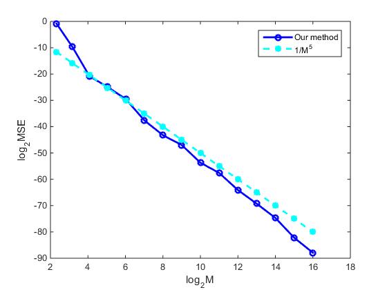
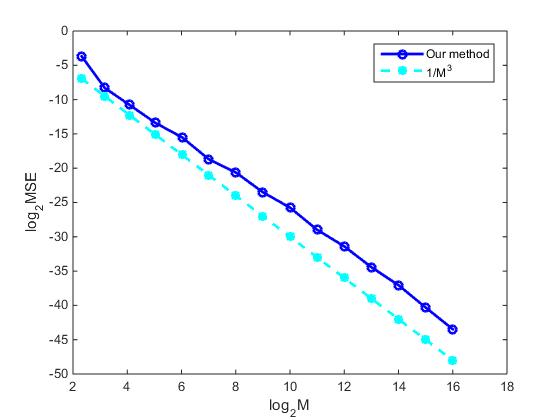
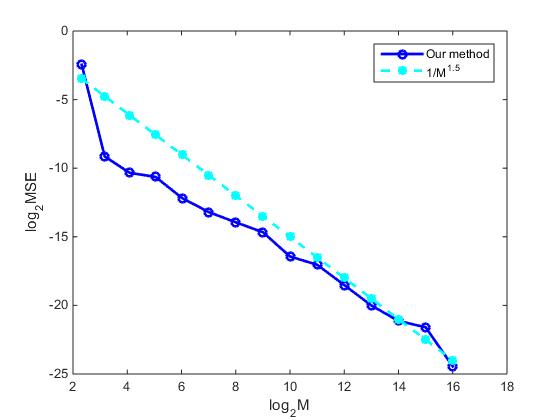
Figure 1: Convergence behavior of our method for $f_{1}$ with $r=0.228\times 2^{k}\,(k=0,1,\dots,14)$ and $L=2^{k}\,(k=1,2,\dots,15)$. The mean squared errors are computed based on $30$ runs.
Refer to caption
Figure 2: Convergence behavior of our method for $f_{2}$ with $r=0.32\times 2^{k}\,(k=0,1,\dots,14)$ and $L=2^{k}\,(k=1,2,\dots,15)$. The mean squared errors are computed based on $30$ runs.
Refer to caption
Figure 3: Convergence behavior of our method for $f_{3}$ with $r=0.42\times 2^{k}(k=0,1,\dots,14)$ and $L=2^{k}\,(k=1,2,\dots,15)$. The mean squared errors are computed based on $30$ runs.

The numerical results for $f_{1}$, achieved through various values of $M$ and $r$, are exhibited in Fig 1 , clearly highlighting that the convergence order of our method surpasses $1/M^{5}$. Similarly, the numerical results for $f_{2}$, displayed in Fig 2, indicate a convergence order approaching $1/M^{3}$. Notably, for both test functions $f_{1}$ and $f_{2}$, our convergence rate is comparable to that reported in [9], achieved without any prior knowledge of the weights.

The numerical results for $f_{3}$, illustrated in Fig 3, reveal that in the $500$-dimensional scenario, the convergence order of our algorithm approaches $M^{1.5}$, marking a substantial improvement over the standard Monte Carlo method, which is of order $1/M$. This superiority remains evident even taking into account the number of repetitions. In fact, to achieve an MSE bound as demonstrated in Eq. (30), it suffices to set $t$ as Ξ˜β€‹((s+1/2)​log⁑M)Ξ˜π‘ 12𝑀\Theta((s+1/2)\log M). As $M$ increases, the impact of Ξ˜β€‹((s+1/2)​log⁑M)Ξ˜π‘ 12𝑀\Theta((s+1/2)\log M) becomes progressively negligible. In contrast, the algorithms presented in [22, 21] tends to converge towards the standard Monte Carlo rate with increasing dimensionality, particularly in the $8$-dimensional scenario, their convergence rate was documented as $1/M^{1.054}$ [22], which served to illustrate their theoretical upper bound of order $1/M^{1+1/d}$ for the scrambled net method.

5 Future Work

We have theoretically developed a nearly optimal integration algorithm for periodic isotropic Sobolev space and weighted Korobov space, which boasts polynomial tractability. However, the RMSE upper bounds for these two spaces involve the factors $\log^{\frac{1}{2}+\frac{s}{d}}(M)$ and $\log^{\frac{1}{2}+s}(M)$ ($M$ denotes sample size), respectively, thus hampering the algorithm’s practical performance. We believe that the integration algorithm combining the median trick with the following random lattice rule can achieve the nearly optimal bounds under the addition of some mild conditions.

$$I(f):=\frac{1}{M}\sum_{0\leq l<M}f_{\eta,M}\bigg{(}\bigg{\{}\frac{z-lH_{M}}{M}\bigg{\}}\bigg{)},$$

where $M$ is a prime, $H_{M}$ and $z$ are drawn from the uniform distribution over $\mathbb{Z}^{d}\cap[1,M)^{d}$ and $\mathbb{Z}^{d}\cap[0,M)^{d}$, respectively, and the definition of $f_{\eta,M}$ is given in Eq.(7). Furthermore, this algorithm has the potential to reduce the logarithmic factors in the upper bound. We leave the exploration of this algorithm for future research.

References

  • [1] Nikolai Sergeevich Bakhvalov. On the approximate calculation of multiple integrals. Journal of Complexity, 31(4):502–516, 2015.
  • [2] Liang Chen. A note on the high-dimensional sparse Fourier transform in the continuous setting. Inverse Problems, 38(3):035008, 2022.
  • [3] Liang Chen and Haixin Jiang. On the information complexity for integration in subspaces of the Wiener algebra. Journal of Complexity, 81:101819, 2024.
  • [4] Liang Chen, Yang Wang, and Haizhang Zhang. Hyper-Gaussian regularized Whittaker–Kotel’nikov–Shannon sampling series. Analysis and Applications, 21(02):329–352, 2023.
  • [5] Nicolas Chopin and Mathieu Gerber. Higher-order Monte Carlo through cubic stratification. SIAM Journal on Numerical Analysis, 62(1):229–247, 2024.
  • [6] Josef Dick. Random weights, robust lattice rules and the geometry of the cbc rc algorithm. Numerische Mathematik, 122:443–467, 2012.
  • [7] Josef Dick. Numerical integration of HΒ¨older continuous, absolutely convergent Fourier, Fourier cosine, and Walsh series. Journal of Approximation Theory, 183:14– 30, 2013.
  • [8] Josef Dick and Takashi Goda. Stability of lattice rules and polynomial lattice rules constructed by the component-by-component algorithm. Journal of Computational and Applied Mathematics, 382:113062, 2021.
  • [9] Josef Dick, Takashi Goda, and Kosuke Suzuki. Component-by-component construction of randomized rank-1 lattice rules achieving almost the optimal randomized error rate. Mathematics of Computation, 91(338):2771–2801, 2022.
  • [10] Josef Dick, Domingo Gomez-Perez, Friedrich Pillichshammer, and Arne Winterhof. Digital inversive vectors can achieve polynomial tractability for the weighted star discrepancy and for multivariate integration. Proceedings of the American Mathematical Society, 145(8):3297–3310, 2017.
  • [11] Josef Dick, Peter Kritzer, and Friedrich Pillichshammer. Lattice Rules: Numerical Integration, Approximation, and Discrepancy. Springer Series in Computational Mathematics, volume 58, Springer, 2022.
  • [12] Josef Dick, Ian H Sloan, Xiaoqun Wang, and Henryk WoΒ΄zniakowski. Good lattice rules in weighted korobov spaces with general weights. Numerische Mathematik, 103:63–97, 2006.
  • [13] Anna C Gilbert, Shan Muthukrishnan, and Martin Strauss. Improved time bounds for near-optimal sparse fourier representations. In Wavelets XI, volume 5914, pages 398–412. SPIE, 2005.
  • [14] Takashi Goda. Polynomial tractability for integration in an unweighted function space with absolutely convergent Fourier series. Proceedings of the American Mathematical Society, 151(09):3925–3933, 2023.
  • [15] Takashi Goda. Strong tractability for multivariate integration in a subspace of the Wiener algebra. arXiv preprint arXiv:2306.01541, 2023.
  • [16] Takashi Goda. A randomized lattice rule without component-by-component construction. arXiv preprint arXiv:2403.02660, 2024.
  • [17] Takashi Goda and Pierre L’ecuyer. Construction-free median quasi-Monte Carlo rules for function spaces with unspecified smoothness and general weights. SIAM Journal on Scientific Computing, 44(4):A2765–A2788, 2022.
  • [18] Takashi Goda, Kosuke Suzuki, and Makoto Matsumoto. A universal median quasi-Monte Carlo integration. SIAM Journal on Numerical Analysis, 62(1):533–566, 2024.
  • [19] Craig Gross, Mark Iwen, Lutz KΒ¨ammerer, and Toni Volkmer. Sparse Fourier transforms on rank-1 lattices for the rapid and low-memory approximation of functions of many variables. Sampling Theory, Signal Processing, and Data Analysis, 20(1):1, 2022.
  • [20] Haitham Hassanieh, Piotr Indyk, Dina Katabi, and Eric Price. Nearly optimal sparse fourier transform. In Proceedings of the forty-fourth annual ACM symposium on Theory of computing, pages 563–578, 2012.
  • [21] Zhijian He and Art B Owen. Extensible grids: uniform sampling on a space filling curve. Journal of the Royal Statistical Society Series B: Statistical Methodology, 78(4):917–931, 2016.
  • [22] Zhijian He and Xiaoqun Wang. On the convergence rate of randomized quasi– Monte Carlo for discontinuous functions. SIAM Journal on Numerical Analysis, 53(5):2488–2503, 2015.
  • [23] Mark A Iwen. Improved approximation guarantees for sublinear-time Fourier algorithms. Applied and Computational Harmonic Analysis, 34(1):57–82, 2013.
  • [24] Mark R Jerrum, Leslie G Valiant, and Vijay V Vazirani. Random generation of combinatorial structures from a uniform distribution. Theoretical Computer Science, 43:169–188, 1986.
  • [25] Lutz KΓ€mmerer, Daniel Potts, and Toni Volkmer. High-dimensional sparse FFT based on sampling along multiple rank-1 lattices. Applied and Computational Harmonic Analysis, 51:225–257, 2021.
  • [26] David Krieg. Tractability of sampling recovery on unweighted function classes. Proceedings of the American Mathematical Society, Series B, 11(12):115–125, 2024.
  • [27] David Krieg and Erich Novak. A universal algorithm for multivariate integration. Foundations of Computational Mathematics, 17:895–916, 2017.
  • [28] Peter Kritzer, Frances Y Kuo, Dirk Nuyens, and Mario Ullrich. Lattice rules with random n achieve nearly the optimal $O(n^{-\alpha-1/2})$ ) error independently of the dimension. Journal of Approximation Theory, 240:96–113, 2019.
  • [29] Robert J Kunsch and Daniel Rudolf. Optimal confidence for Monte Carlo integration of smooth functions. Advances in Computational Mathematics, 45(5):3095–3122, 2019.
  • [30] Frances Y Kuo, Dirk Nuyens, and Laurence Wilkes. Random-prime–fixed-vector randomised lattice-based algorithm for high-dimensional integration. Journal of Complexity, 79:101785, 2023.
  • [31] Wojciech Niemiro and Piotr Pokarowski. Fixed precision MCMC estimation by median of products of averages. Journal of Applied Probability, 46(2):309–329, 2009.
  • [32] Dirk Nuyens and Laurence Wilkes. A randomised lattice rule algorithm with pre-determined generating vector and random number of points for korobov spaces with $0<\alpha\leq 1/2$. arXiv preprint arXiv:2308.03138, 2023.
  • [33] Zexin Pan and Art Owen. Super-polynomial accuracy of one dimensional randomized nets using the median of means. Mathematics of Computation, 92(340):805–837, 2023.
  • [34] Zexin Pan and Art Owen. Super-polynomial accuracy of multidimensional randomized nets using the median-of-means. Mathematics of Computation, 2024.
  • [35] Mario Ullrich. A Monte Carlo method for integration of multivariate smooth functions. SIAM Journal on Numerical Analysis, 55(3):1188–1200, 2017.