Can the noble metals (Au, Ag and Cu) be superconductors?

Abstract

It is common knowledge that noble metals are excellent conductors but do not exhibit superconductivity. On the other hand, quantum confinement in thin films has been consistently shown to induce a significant enhancement of the superconducting critical temperature in several superconductors. It is therefore an important fundamental question whether ultra-thin film confinement may induce observable superconductivity in non-superconducting metals. We present a generalization, in the Eliashberg framework, of a BCS theory of superconductivity in good metals under thin-film confinement. By numerically solving these new Eliashberg-type equations, we find the dependence of the superconducting critical temperature on the film thickness $L$. This parameter-free theory predicts a maximum increase in the critical temperature for a specific value of the film thickness, which is a function of the number of free carriers in the material. Exploiting this fact, we predict that ultra-thin films of gold, silver and copper of suitable thickness could be superconductors at low but experimentally accessible temperatures. We demonstrate that this is a fine-tuning problem where the thickness must assume a very precise value, close to half a nanometer.

It is well known that the three best conducting metals, Au Ag and Cu, are also among the few metallic elements that are not superconductors even when subjected to high pressures Khan and Raub (1975); Buzea and Robbie (2004). In this article we demonstrate, by exploiting the phenomenon of quantum confinement, that it is possible to make these materials superconducting as long as they are cast into ultra-thin films of a very well-defined thickness. The superconducting critical temperatures will still be low but not so low that they cannot be measured experimentally. The standard one-infinite-band s-wave Eliashberg theory Eliashberg (1960); Carbotte (1990) is a powerful tool to compute all superconductive properties of elemental superconductors Carbotte (1990) such as as Pb, Sn, Al etc. In this regard, many studies have been devoted to rationalizing the dependence of the superconducting critical temperature $T_{c}$ on confinement and on the thin film thickness $L$ Blatt and Thompson (1963); Arutyunov et al. (2019); Valentinis et al. (2016); Bianconi and Missori (1994); Eom et al. (2006); Qin et al. (2009). In the past, due to the vapor-deposition technique Buckel and Hilsch (1954), superconducting thin films were mostly amorphous while nowadays, thanks to the modern preparation techniques, also crystalline thin films can be fabricated. Early numerical studies based on BCS theory Blatt and Thompson (1963) suggested a possible enhancement of $T_{c}$ upon decreasing the film thickness $L$, although a mechanistic explanation has remained elusive. More recently, experiments on ordered thin films Eom et al. (2006); Qin et al. (2009); van Weerdenburg et al. (2023), besides the above mentioned regime of $T_{c}$ enhancement upon reducing $L$, have also highlighted a second regime at lower (nanometric and sub-nanometric) thicknesses $L$, where, instead, $T_{c}$ grows with increasing $L$. This behaviour results, overall, in a non-monotonic trend with a peak or maximum of $T_{c}$ as a function of $L$. Travaglino and Zaccone in a recent paper Travaglino and Zaccone (2023) developed the first fully analytical theory of confinement effects on superconductivity of thin films in the framework of the simplified weak-coupling BCS formalism. The mathematical predictions were verified for experimental data of crystalline thin films and were able to reproduce the trend of $T_{c}$ vs $L$, including the maximum of $T_{c}$ at $L=L_{c}=(2\pi/n)^{1/3}$, where $n$ is the concentration of free carriers. This maximum coincides with a topological transition of the Fermi surface, from the spherical-like Fermi surface of bulk metals to a non-trivial topology with homotopy group $\simeq\mathbb{Z}$. This topological transition marks the change from a situation where free electrons get crowded at the Fermi level upon decreasing the film thickness (due to the growth of hole pockets internal to the spherical Fermi surface) to a regime of strong confinement where the new topology of the Fermi surface allows for spreading out the free electron energy states at the surface. This phenomenon provides a mechanistic explanation to the maximum in $T_{c}$ vs thickness $L$ observed experimentally.

In this paper, we formulate a generalized Eliashberg theory of strong-coupling superconductivity of noble-metal thin films, that takes into account effects of quantum confinement on the free carriers, as well as a realistic electron-phonon spectral density. To this aim, we use a generalization of the standard s-wave one-band Eliashberg theory Eliashberg (1960) where the new Eliashberg equations are more complex than the usual ones, because the normal density of states (DOS) is not approximated by its value at the Fermi level. This theory is shown to yield predictions for Au, Ag and Cu thin films, with no adjustable parameters. Moreover, the calculations predict that the noble metals Au, Ag and Cu, become superconductors at precise values of the film thickness. These predictions have the potential to change our fundamental understanding of superconductivity in nanostructured materials, with many relevant technological applications ranging from Josephson junctions to quantum computing.

The Eliashberg equations, in their simpler version (one infinite band with isotropic order parameter), are given in terms of the gap function $\Delta(i\omega_{n})$ and renormalization function $Z(i\omega_{n})$ Carbotte (1990); Marsiglio and Carbotte (2008); Allen and Mitrović (1983); Parks (1969) (ed.); Marsiglio (1992); Ummarino (2013); Margine and Giustino (2013). When the Migdal’s theorem holds Ummarino and Gonnelli (1997), they read as:

$$\Delta(i\omega_{n})Z(i\omega_{n})=\pi T\sum_{\omega_{n^{\prime}}}\frac{\Delta(i\omega_{n^{\prime}})}{\sqrt{\omega_{n^{\prime}}^{2}+\Delta^{2}(i\omega_{n})}}\times$$

$$\big{[}\lambda(i\omega_{n^{\prime}}-i\omega_{n})-\mu^{*}(\omega_{c})\theta(\omega_{c}-|\omega_{n^{\prime}}|)\big{]},$$

$$Z(i\omega_{n}) =1+\frac{\pi T}{\omega_{n}}\sum_{\omega_{n^{\prime}}}\frac{\omega_{n^{\prime}}}{\sqrt{\omega_{n^{\prime}}^{2}+\Delta^{2}(i\omega_{n})}}\lambda(i\omega_{n^{\prime}}-i\omega_{n})$$ (1)

where $\mu^{*}(\omega_{c})$ is the Coulomb pseudopotential that depends, in a weak way, on a cut-off energy $\omega_{c}$ ($\omega_{c}>3\Omega_{max}$ where $\Omega_{max}$ is the maximum phonon or Debye energy) Allen and Mitrović (1983), and $\theta(\omega_{c}-|\omega_{n^{\prime}}|)$ is the Heaviside function. $\lambda(i\omega_{n^{\prime}}-i\omega_{n})$ is a function related to the electron-phonon spectral function $\alpha^{2}F(\Omega)$ through the relation

$$\lambda(i\omega_{n^{\prime}}-i\omega_{n})=2\int_{0}^{\infty}\frac{\Omega\alpha^{2}F(\Omega)d\Omega}{\Omega^{2}+(\omega_{n^{\prime}}-\omega_{n})^{2}}.$$ (2)

The strength of the electron-phonon coupling is given by the electron-phonon coupling parameter $\lambda=2\int_{0}^{\infty}\frac{\alpha^{2}F(\Omega)d\Omega}{\Omega}$. In general, it is impossible to find exact analytical solutions of Eliashberg’s equations except for the case of extreme strong-coupling ($\lambda>10$) Carbotte (1990). Hence, we solve them numerically with an iterative method until numerical convergence is reached. This numerical procedure is easy to perform in the formulation on the imaginary axis, but less so on the real axis. The $T_{c}$ can be calculated either by solving an eigenvalue equation or, more easily, by giving a very small test value to the superconducting gap and then by checking at which temperature the solution converges. In this way, a precision in the $T_{c}$ value is obtained that is much higher than the experimental confidence interval. The simplest thing to do to generalize the Eliashberg equations is to remove the infinite band approximation (which works very well for most metals in the bulk state) and to no longer approximate the normal DOS as a function of energy with its value at the Fermi level. By removing these approximations, the Eliashberg equations become slightly more complex and they become four equations Allen and Mitrović (1983). However, in the particular case where the DOS is symmetrical with respect to the Fermi level ($N(\varepsilon)=N(-\varepsilon)$), it is possible to simplify the theory in the way that the self energy terms remain just two, $Z(i\omega_{n})$ and $\Delta(i\omega_{n})Z(i\omega_{n})$, and the equations read as Schachinger and Carbotte (1983); Pickett (1980)

$$\Delta(i\omega_{n})Z(i\omega_{n})= \pi T\sum_{\omega_{n^{\prime}}}\frac{\Delta(i\omega_{n^{\prime}})}{\sqrt{\omega_{n^{\prime}}^{2}+\Delta^{2}(i\omega_{n})}}[\frac{N(i\omega_{n^{\prime}})+N(-i\omega_{n^{\prime}})}{2}]\times$$

$$\big{[}\lambda(i\omega_{n^{\prime}}-i\omega_{n})-\mu^{*}(\omega_{c})\theta(\omega_{c}-|\omega_{n^{\prime}}|)\big{]}\frac{2}{\pi}\arctan(\frac{W}{2Z(i\omega_{n^{\prime}})\sqrt{\omega_{n^{\prime}}^{2}+\Delta^{2}(i\omega_{n^{\prime}})}}),$$ (3)

$$Z(i\omega_{n})= 1+\frac{\pi T}{\omega_{n}}\sum_{\omega_{n^{\prime}}}\frac{\omega_{n^{\prime}}}{\sqrt{\omega_{n^{\prime}}^{2}+\Delta^{2}(i\omega_{n})}}[\frac{N(i\omega_{n^{\prime}})+N(-i\omega_{n^{\prime}})}{2}]\lambda(i\omega_{n^{\prime}}-i\omega_{n})\frac{2}{\pi}\arctan(\frac{W}{2Z(i\omega_{n^{\prime}})\sqrt{\omega_{n^{\prime}}^{2}+\Delta^{2}(i\omega_{n^{\prime}})}})$$ (4)

where $N(\pm i\omega_{n^{\prime}})=N(\pm Z(i\omega_{n^{\prime}})\sqrt{(\omega_{n^{\prime}})^{2}+\Delta^{2}(i\omega_{n^{\prime}})})$ and the bandwidth $W$ is equal to half the Fermi energy, $E_{F}/2$.

When the system is confined along one of the three spatial directions, such as in thin films, the DOS features two different regimes depending on the film thickness $L$ Travaglino and Zaccone (2023): when $L>L_{c}$ and $E_{F}>\varepsilon^{*}$, the DOS has the following form $N(\varepsilon)=N(0)C[\vartheta(\varepsilon^{*}-\varepsilon)\sqrt{\frac{E_{F}}{\varepsilon^{*}}}\frac{|\varepsilon|}{E_{F}}+\vartheta(\varepsilon-\varepsilon^{*})\sqrt{\frac{|\varepsilon|}{E_{F}}}]$ where $C=(1+\frac{1}{3}\frac{L_{c}^{3}}{L^{3}})^{1/3}$, $\varepsilon^{*}=\frac{2\pi^{2}\hbar^{2}}{mL^{2}}$, $L_{c}=(\frac{2\pi}{n_{0}})^{1/3}$, $m$ is the electron mass, $L$ is the film thickness, $n_{0}$ is the density of carriers and $E_{F,bulk}$ is the Fermi energy of the bulk material. In this case, it is possible to demonstrate the following relations Travaglino and Zaccone (2023):

$$E_{F} =C^{2}E_{F,bulk}$$ (5)

$$N(E_{F}) =CN(E_{F,bulk})=CN(0),$$ (6)

with $N(E_{F,bulk})=\frac{V(2m)^{3/2}}{2\pi^{2}\hbar^{3}}\sqrt{E_{F,bulk}}$. In the regime $\epsilon<\epsilon^{*}$, the DOS has a new, linear dependence on the energy, in contrast with the standard square-root dependence which is retrieved for $\epsilon>\epsilon^{*}$ Travaglino and Zaccone (2023). We can summarize the main features that change in this version of the Eliashberg equations: i) the DOS will no longer be a constant but a function of energy; ii) the electron-phonon interaction is a function of film thickness $L$, via $\lambda=C\lambda^{bulk}$; iii) the value of the Fermi energy is also a function of the film thickness $L$: $E_{F}=C^{2}E_{F,bulk}$. Of course, in the symmetric case discussed above, it is $W=E_{F}/2$; iv) the Coulomb pseudopotential $\mu^{*}$ also depends on the film thickness via $\mu^{*}=\frac{C\mu_{bulk}}{1+\mu_{bulk}\ln(E_{F}/\omega_{c})}$ where $\mu_{bulk}=\frac{\mu^{*}_{bulk}}{1-\mu^{*}_{bulk}\ln(E_{F,bulk}/\omega_{c})}$. Instead, when $L<L_{c}$ and $E_{F}<\varepsilon^{*}$, we have Travaglino and Zaccone (2023):

$$N(\varepsilon)=C^{\prime}N(0)\sqrt{\frac{E_{F}}{\varepsilon^{*}}}\frac{\varepsilon}{E_{F}}$$ (7)

where $N(\varepsilon=E_{F})=C^{\prime}N(0)$, $E_{F}=C^{\prime 2}E_{F,bulk}$ and $C^{\prime}=\frac{2}{\sqrt{L}}(\frac{8\pi}{3})^{2/3}\frac{1}{(n(2\pi)^{3})^{1/6}}$. In this regime, the DOS is given by Travaglino and Zaccone (2023): $N(\varepsilon)=\sqrt{\frac{E_{F}}{\varepsilon^{*}}}\frac{|\varepsilon|}{E_{F}}$. The electron-phonon coupling and the Coulomb pseudopotential become thickness-dependent through $C^{\prime}$:

$$\lambda=C^{\prime}\lambda^{bulk},\leavevmode\nobreak\ \leavevmode\nobreak\ \leavevmode\nobreak\ \mu^{*}=\frac{C^{\prime}\mu_{bulk}}{1+\mu_{bulk}\ln(E_{F}/\omega_{c})}.$$ (8)

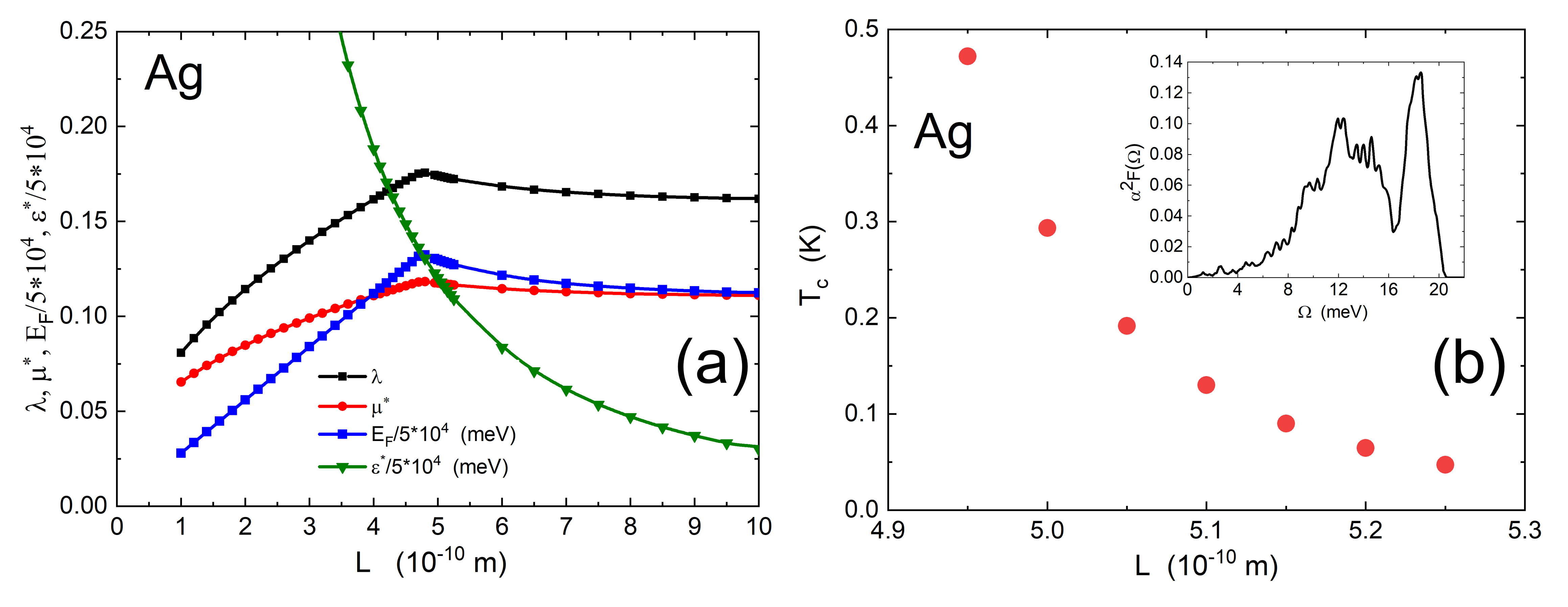
Figure 1: Panel (a) shows the physical parameters used in the theory for silver (Ag) films: $\lambda$ (dark line and squares), $\mu^{*}$ (red line and circles), $E_{F}/5\cdot 10^{4}$ (blue line and up triangles), $\varepsilon^{*}/5\cdot 10^{4}$) (green line and down triangles). All the parameters are plotted as a function of the film thickness $L$. Panel (b) shows the critical temperature $T_{c}$ versus film thickness $L$ for silver (Ag): full red circles represent the numerical solutions of the Eliashberg equations. In the inset, the Eliashberg electron-phonon spectral function of silver is shown, from Ref. Giri et al. (2020).

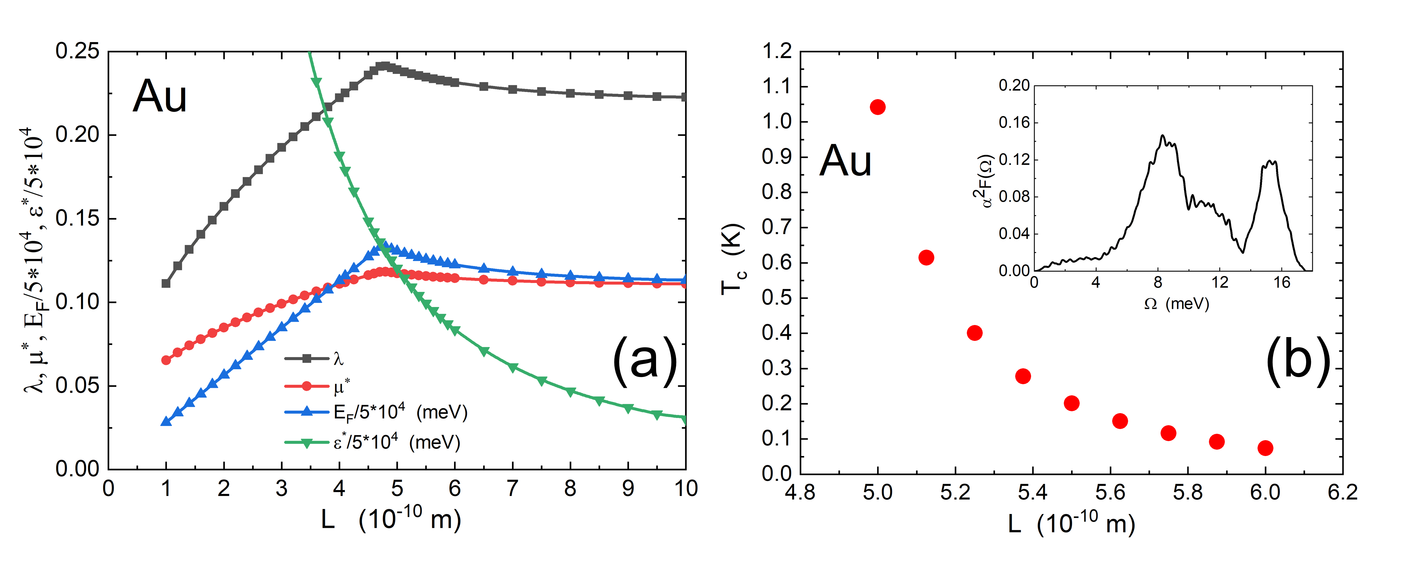
Figure 2: Panel (a) shows the physical parameters used in the theory for gold (Au) films: $\lambda$ (dark line and squares), $\mu^{*}$ (red line and circles), $E_{F}/5\cdot 10^{4}$ (blue line and up triangles), $\varepsilon^{*}/5\cdot 10^{4}$) (green line and down triangles). All parameters are plotted as a function of the film thickness $L$. Panel (b) shows the critical temperature $T_{c}$ versus film thickness $L$ for gold (Au): full red circles represent the numerical solutions of Eliashberg equations. In the inset, the Eliashberg electron-phonon spectral function of gold is shown, from Ref. Giri et al. (2020).

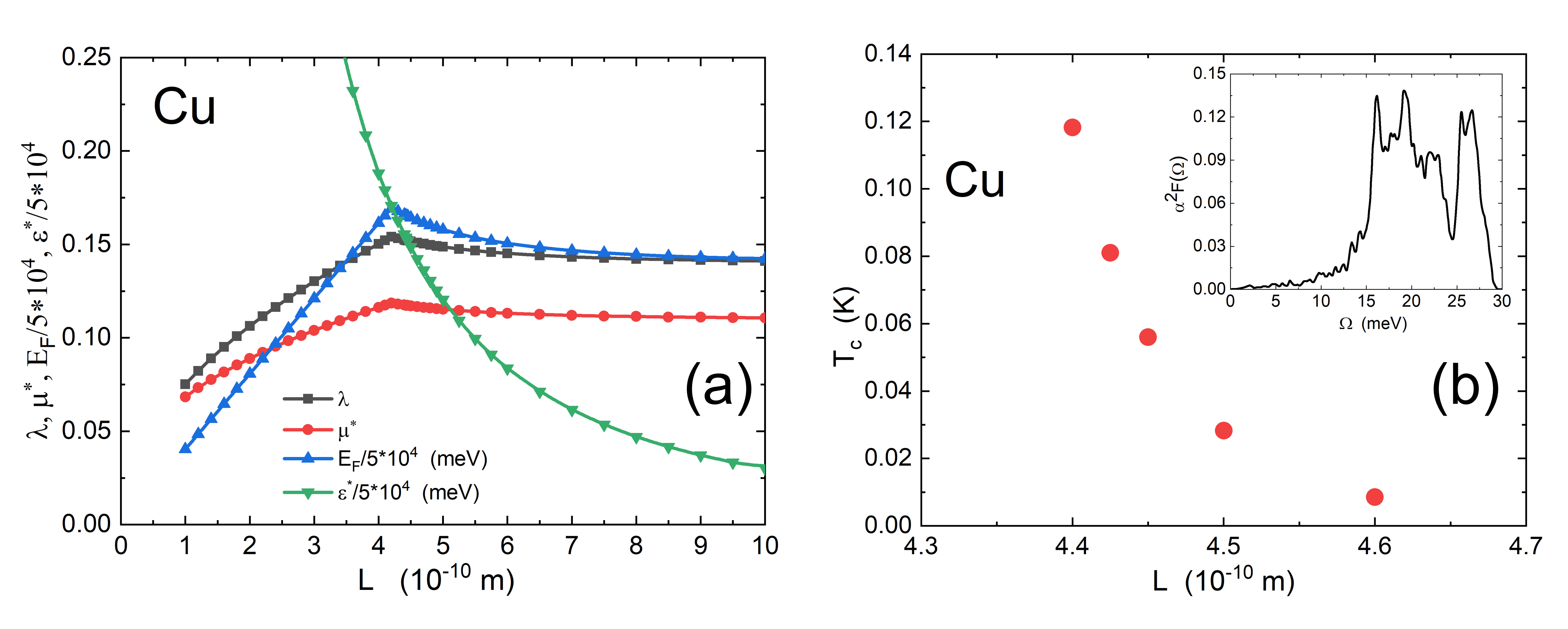
Figure 3: Panel (a) shows the values of the physical parameters used in the theory for copper (Cu) films: $\lambda$ (dark line and squares), $\mu^{*}$ (red line and circles), $E_{F}/5\cdot 10^{4}$ (blue line and up triangles), $\varepsilon^{*}/5\cdot 10^{4}$) (green line and down triangles). All the parameters are plotted as a function of the film thickness $L$. Panel (b) shows the critical temperature $T_{c}$ versus film thickness $L$ for copper (Cu): full red circles represent the numerical solutions of Eliashberg equations. In the inset, the Eliashberg electron-phonon spectral function of copper is shown, from Ref. Giri et al. (2020).

It is well known that all three noble metals (Au, Ag, Cu) have a very weak electron-phonon coupling ($\lambda<0.25$), which does not allow them to be bulk superconductors. However, if we consider very thin films with a thickness very close to the critical length $L_{c}$, which is of the order of 5 Å (0.5 nm), our calculations using the above theory show that the electron-phonon interaction is greatly enhanced. Therefore, the possibility exists that, in a narrow range of thickness, the noble metal film becomes superconducting. This is the scenario revealed by our calculations in Figs. 1-3.

Let us start by considering the case of silver and examine how the fundamental parameters vary around the critical thickness $L_{c}$. In Fig. 1(a) the physical quantities of silver used in the theoretical calculations are plotted as functions of the film thickness $L$. The bulk electron-phonon spectral function of silver Giri et al. (2020) with $\lambda_{bulk,0}=0.16$ is shown in the inset of Fig. 1(b). The bulk value of the Coulomb pseudopotential Giri et al. (2020) is $\mu^{*}(\omega_{c})=0.11$, the cut-off energy is $\omega_{c}=75$ meV and the maximum electronic energy is $\omega_{max}=80$ meV. The values of the bulk Fermi energy and carrier density are respectively $E_{F,bulk}=5490$ meV and $n_{0}=0.0586\cdot 10^{30}$ $m^{-3}$. This produces a critical thickness $L_{c}=4.75$ Å. As we can see from Fig. 1(a), precisely around this critical thickness value, the coupling constant $\lambda$ has a slight increase. To check whether this increase is sufficient to produce the superconducting state, we solve the modified Eliashberg equations and calculate the critical temperature $T_{c}$. The result is shown in Fig. 1(b). We find that, for the film thickness $L=5.00$ Å (very close to the critical value $L_{c}=4.75$ Å) the material becomes a superconductor with $T_{c}=0.294$ $K$. We notice that the thickness range that allows superconductivity to exist is quite narrow, which can be understood based on the underlying topological transition Travaglino and Zaccone (2023). We now turn to the case of gold. In Fig. 2(a) the physical quantities for Au used in the theory are shown as functions of the film thickness. The bulk electron phonon spectral function of gold Giri et al. (2020) with $\lambda_{bulk,0}=0.22$ is shown in the inset of Fig. 2(b). The bulk value of the Coulomb pseudopotential Giri et al. (2020) is $\mu^{*}(\omega_{c})=0.11$, the cut-off energy is $\omega_{c}=55$ meV and the maximum electronic energy is $\omega_{max}=60$ meV. The values of the bulk Fermi energy and carrier density are, respectively, $E_{F,bulk}=5530$ meV and $n_{0}=0.0590\cdot 10^{30}$ $m^{-3}$. This produces a critical thickness $L_{c}=4.74$ Å. For Au, we find that, for the thickness $L=5.00$ Å which is close to the critical value $L_{c}=4.74$ Å, the material becomes a superconductor with $T_{c}=1.042$ $K$. Also in this case, the thickness range that allows superconductivity to be observed is narrow. As the last case, we study copper (Cu). In Fig. 3(a), some typical physical quantities of copper used in the theory are shown as functions of the film thickness $L$. The bulk electron-phonon spectral function of copper Giri et al. (2020) with $\lambda_{bulk,0}=0.14$ is shown in the inset of Fig. 3(b). The bulk value of the Coulomb pseudopotential Giri et al. (2020) is $\mu^{*}(\omega_{c})=0.11$ (the cut-off energy is $\omega_{c}=90$ meV and the maximum electronic energy is $\omega_{max}=100$ meV). The values of the bulk Fermi energy and carrier density are, respectively, $E_{F,bulk}=7000$ meV and $n_{0}=0.0847\cdot 10^{30}$ $m^{-3}$. For copper we find that, if the thickness is $L=4.40$ Å, i.e. close to the critical value $L_{c}=4.20$ Å, the material becomes a superconductor with $T_{c}=0.118$ $K$.

We notice that as soon as we move away from the critical value $L_{c}$ of film thickness, the $T_{c}$ abruptly goes to very small values, which we are not able to calculate as it is too time-consuming for the code to reach convergence.

In conclusion, we have studied a new generalization of the Eliashberg equations which include the crucial effect of quantum confinement, to compute the superconducting properties of thin films of noble metals, in a fully quantitative way and with no free parameters. Upon decreasing the film thickness, the formation of hole pockets growing inside the Fermi sea Travaglino and Zaccone (2023) leads to the ”crowding” of electronic states at the Fermi level, which can significantly increase the electron-phonon coupling, and hence the $T_{c}$. Surprisingly, the theoretical predictions reveal the possibility that films of Au, Ag, and Cu with a thickness close to 0.5 nm become superconducting. Particularly striking is the case of gold (Au), which can reach a superconducting critical temperature of $T_{c}\approx 1.1$ $K$, which is comparable to that of bulk aluminum, i.e. the most used material for Josephson junctions. These predictions open up unprecedented new avenues for both the fundamental understanding of superconductivity as well as for many technological applications, from superconducting logic to quantum computing.

.1 Acknowledgments

A.Z. gratefully acknowledges funding from the European Union through Horizon Europe ERC Grant number: 101043968 “Multimech”, from US Army Research Office through contract nr. W911NF-22-2-0256, and from the Niedersächsische Akademie der Wissenschaften zu Göttingen in the frame of the Gauss Professorship program.

References

- Khan and Raub (1975) H. R. Khan and C. J. Raub, Gold Bulletin 8, 114 (1975).
- Buzea and Robbie (2004) C. Buzea and K. Robbie, Superconductor Science and Technology 18, R1 (2004).
- Eliashberg (1960) G. M. Eliashberg, Sov. Phys. JETP 11, 696 (1960).
- Carbotte (1990) J. P. Carbotte, Rev. Mod. Phys. 62, 1027 (1990).
- Blatt and Thompson (1963) J. M. Blatt and C. J. Thompson, Phys. Rev. Lett. 10, 332 (1963).
- Arutyunov et al. (2019) K. Y. Arutyunov, E. A. Sedov, I. A. Golokolenov, V. V. Zav’yalov, G. Konstantinidis, A. Stavrinidis, G. Stavrinidis, I. Vasiliadis, T. Kekhagias, G. P. Dimitrakopulos, F. Komninu, M. D. Kroitoru, and A. A. Shanenko, Physics of the Solid State 61, 1559 (2019).
- Valentinis et al. (2016) D. Valentinis, D. van der Marel, and C. Berthod, Phys. Rev. B 94, 054516 (2016).
- Bianconi and Missori (1994) A. Bianconi and M. Missori, Journal de Physique I 4, 361 (1994).
- Eom et al. (2006) D. Eom, S. Qin, M.-Y. Chou, and C. K. Shih, Phys. Rev. Lett. 96, 027005 (2006).
- Qin et al. (2009) S. Qin, J. Kim, Q. Niu, and C.-K. Shih, Science 324, 1314 (2009).
- Buckel and Hilsch (1954) W. Buckel and R. Hilsch, Zeitschrift für Physik 138, 109 (1954).
- van Weerdenburg et al. (2023) W. M. van Weerdenburg, A. Kamlapure, E. H. Fyhn, X. Huang, N. P. van Mullekom, M. Steinbrecher, P. Krogstrup, J. Linder, and A. A. Khajetoorians, Science Advances 9, eadf5500 (2023), https://www.science.org/doi/pdf/10.1126/sciadv.adf5500 .
- Travaglino and Zaccone (2023) R. Travaglino and A. Zaccone, Journal of Applied Physics 133, 033901 (2023).
- Marsiglio and Carbotte (2008) F. Marsiglio and J. P. Carbotte, “Electron-phonon superconductivity,” in Superconductivity: Conventional and Unconventional Superconductors, edited by K. H. Bennemann and J. B. Ketterson (Springer Berlin Heidelberg, Berlin, Heidelberg, 2008) pp. 73–162.
- Allen and Mitrović (1983) P. B. Allen and B. Mitrović, “Theory of superconducting tc,” (Academic Press, 1983) pp. 1–92.
- Parks (1969) (ed.) R. D. Parks (ed.), Superconductivity, vol. 1 (Marcel Dekker, New York, 1969) p. 67.
- Marsiglio (1992) F. Marsiglio, Journal of Low Temperature Physics 87, 659 (1992).
- Ummarino (2013) G. Ummarino, “Eliashberg theory,” in Emergent Phenomena in Correlated Matter, edited by E. Pavarini, E. Koch, and U. Schollwoeck (Forschungszentrum Julich GmbH and Institute for Advanced Simulations, Julich, 2013) pp. 13.1–13.36.
- Margine and Giustino (2013) E. R. Margine and F. Giustino, Phys. Rev. B 87, 024505 (2013).
- Ummarino and Gonnelli (1997) G. A. Ummarino and R. S. Gonnelli, Phys. Rev. B 56, R14279 (1997).
- Schachinger and Carbotte (1983) E. Schachinger and J. P. Carbotte, Journal of Physics F: Metal Physics 13, 2615 (1983).
- Pickett (1980) W. E. Pickett, Phys. Rev. B 21, 3897 (1980).
- Giri et al. (2020) A. Giri, M. Tokina, O. Prezhdo, and P. Hopkins, Materials Today Physics 12, 100175 (2020).