KPP fronts in shear flows with cut-off reaction rates
Abstract
We consider the effect of a shear flow which has, without loss of generality, a zero mean flow rate, on a Kolmogorov–Petrovskii–Piscounov (KPP) type model in the presence of a discontinuous cut-off at concentration . In the long-time limit, a permanent form travelling wave solution is established which, for fixed , is unique. Its structure and speed of propagation depends on (the strength of the flow relative to the propagation speed in the absence of advection) and (the square of the front thickness relative to the channel width). We use matched asymptotic expansions to approximate the propagation speed in the three natural cases , and , with particular associated orderings on , whilst remains fixed. In all the cases that we consider, the shear flow enhances the speed of propagation in a manner that is similar to the case without cut-off (). We illustrate the theory by evaluating expressions (either directly or through numerical integration) for the particular cases of the plane Couette and Poiseuille flows.
Keywords: reaction-diffusion, permanent form travelling waves, cut-off nonlinearity, shear flow, asymptotic expansions.
1 Introduction
We investigate travelling fronts for cut-off reaction–diffusion equations evolving in an infinite channel in the presence of a shear flow. The model equation that we consider describes the spatio-temporal evolution of the scalar function denoting the concentration field of a dissolved species, and takes the non-dimensional generic form
| (IBVPa) | |||
| Here, the dimensionless spatial coordinate has been obtained by scaling with the channel width whilst the dimensionless spatial coordinate has been obtained by scaling with the diffusive length scale where is the molecular diffusivity and is the reaction timescale. The latter has also been used to introduce the dimensionless time . The cut-off reaction function is given by | |||
| (IBVPb) | |||
| where is a normalised KPP-type reaction function, named after the classical work by Fisher [11] and Kolmogorov, Petrovskii, and Piskunov [15], which satisfies | |||
| (IBVPc) | |||
| Thus the reaction is effectively deactivated at points where the concentration lies at or below a threshold value . For convenience throughout, we introduce the shorthand notation , the limiting value from above of at . A prototypical example of such a KPP reaction function is the Fisher reaction function [11] given by . The flow function satisfies . It corresponds to the -component of a unidirectional, zero-mean, steady incompressible shear flow with fluid velocity field | |||
| (IBVPd) | |||
| Equation (IBVPa) involves two non-dimensional parameters | |||
| where is the characteristic speed of the (dimensional) flow. They respectively measure the strength of advective fluid velocity relative to the front speed (in the absence of advection), and the square of the front thickness (in the absence of advection) to the square of the channel width. We focus on two-dimensional straight infinite channel domains with Neumann boundary conditions at the domain walls, | |||
| (IBVPe) | |||
| so that there is no flux of across the wall of the domain. These are supplemented by the initial conditions and far field boundary conditions, namely, | |||
| (IBVPf) | |||
| with these limits being uniform for and , for any . Here is the usual Heavyside function. In what follows we will refer to the initial boundary value problem specified by the above equations as (IBVP). | |||
1.1 Background and related works
The (IBVP) was first considered by Brunet and Derrida [3] in the absence of a background flow that is, when . They proposed it as a model to provide insight into the spreading of discrete systems of interacting chemical and biological particles in homogeneous environments. They conjectured that discreteness in concentration values can be represented by an effective cut-off concentration , where may be viewed as the effective mass of a single particle. The idea is that for , diffusion dominates over growth. It is now recognised, following previous work by Tisbury and the authors [25], that the solution to (IBVP) in the absence of a background flow evolves at large times to a permanent form traveling wave (PTW) solution and propagation speed in the sense that there exist functions and such that
| (1) |
as uniformly for , with being exponentially small in as and a similar, spatially uniform, rate of convergence in the second limit in (1). Tisbury and the authors [24] showed that the PTW solution is, for each and KPP function , unique (up to translation), monotone decreasing and positive, with and . Its propagation speed is, for fixed , uniquely determined by the existence of a heteroclinic connection in the phase plane which connects the equilibrium point , as , to the equilibrium point as (the translational invariance is then fixed by requiring that ). An explicit expression for is not available. However, it is straightforward to demonstrate that is a continuous, monotone decreasing function of , with as and as [24] , where is the minimum propagation speed of the PTW solution in the absence of cut-off (). Its asymptotic form can be approximated in the limits of and . In the first limit, Brunet and Derrida [3] predicted that the value of is strongly influenced by the presence of a cut-off, with
| (2) |
so that in this limit, the difference between and is only logarithmically small in . This behaviour was rigorously verified by Dumortier, Popovic and Kaper [8] using geometric desingularization. Higher order corrections were obtained by Tisbury and the authors [24] using matched asymptotic expansions. The behaviour of as is in contrast with the behaviour of as , in which case it was established in [24] that
| (3) |
and so now vanishing algebraically in . There are no equivalent results for the spatially heterogenous version of (IBVP) (.
In this paper our aim is to understand how advection by a shear flow influences the shape of the PTW solution and its propagation speed. This understanding is important due to the fact that in a wide variety of environmental and engineering applications, associated chemical or biological reactive species are transported by fluid flows, with the simplest non-trivial flows being shear flows. In this case, it is natural to anticipate curved PTW solutions of the form and propagation speed , where . The functions and now satisfy
| (4) |
as uniformly for with as uniformly in . The question of existence of curved PTW solutions for KPP reactions without cut-off (that is, ) and shear flows with bounded cross-sections and Neumann boundary conditions was considered in detail by Berestycki and Nirenberg [2]. They used the approach of sub- and super-solutions on the associated semilinear elliptic boundary value problem to establish that a unique PTW solution exists for each propagation , where is the (positive) minimum available propagation speed. This PTW solution is monotone decreasing in and has and , uniformly for . A number of works [12, 18, 22] have shown that in fact, for KPP reactions without cut-off, the solution to the (IBVP) approaches that PTW with minimum speed .
The elliptic boundary value problem whose solution provides the curved PTW presents little immediate and direct information about the quantitative dependence of the propagation speed on the parameters and the details of the profiles of the advective flow and reaction functions. A first characterization of the propagation speed was derived by Gärtner and Freidlin [13] for KPP reactions using probabilistic arguments. This variational characterization expressed in terms of the principal eigenvalue of a certain linear eigenvalue problem that depends on , and . Thus, depends on the structure of but not the detailed structure of (other than it satisfying the KPP conditions). An alternative characterization of was subsequently derived by Berestycki and Nirenberg [2] in terms of a quadratic linear eigenvalue problem, where is determined by the requirement that the two principal eigenvalues are equal (the equivalence of the two characterizations is shown in [28]). A variational characterization was developed in [23] for the case of bistable and combustion type nonlinearity.
The eigenvalue problem determining the speed of propagation of the curved PTW solution for KPP reaction functions without cut-off is readily solved numerically. An exact analytical solution is, however, not available even for simple shear flows. It can nevertheless be analysed in asymptotic limits of the two parameters and . For a channel width that is comparable to the advectionless front scale thickness, i.e. when , it can be shown that a shear flow enhances the speed of propagation, with the enhancement being monotonic in [1]. Further asymptotic results obtained in [21] and [1] respectively provide explicit expressions for with
| (5) |
where the constant was determined in [14]. For a channel width that is much smaller than the advectionless front scale thickness, i.e. when , is, at leading order, proportional to the square root of the effective diffusivity of the advection–diffusion problem [23] so that
| (6a) | |||
| uniformly for . An explicit form for can be obtained using homogenization (see, for example, [16, 4]) which yields | |||
| (6b) | |||
which holds uniformly for . Here, . In the opposite limit, when the channel width is much larger than the advectionless front scale thickness, i.e. when , the PTW solutions are sharp-fronted and can be approximated by a single curve where all the reaction takes place. Majda and Souganidis [17] (see also [12, Ch. 6]) showed that a distinguished regime arises for in which case the propagation speed satisfies [10, 29, 26]
| (7) |
A complete description of as can be readily deduced from the analysis in [14].
A natural question is to what extent the above results apply in the presence of a cut-off in the reaction.
1.2 Main results and paper structure
In this paper we consider (IBVP) in a number of natural asymptotic limits on the parameters and , with fixed. One feature which we concentrate on, amongst others, is the existence of PTW solutions, and the detailed form of the associated propagation speed, , which, for , is unique. We use the theory of matched asymptotic expansions to establish the limiting form of (IBVP) and/or the associated PTW theory, and subsequently obtain expressions for and the boundary of the interface where , in the three natural cases of , and . Our main conclusions are that for with , the solution to (IBVP) is, at leading order, described by an effective equation devoid of advection with molecular diffusivity replaced by the effective diffusivity (6b). Thus, is at leading order enhanced by the shear flow by a factor proportional to the square root of . For we consider each of the complementary orderings and , and find that is at leading order given by , the speed of propagation in the absence of a flow with determined solely by the structure of the flow and the value of . The higher order correction to the speed is of when , initially increasing from zero as , until it achieves a maximum point located at a value . Thereafter it is decreasing with increasing , becoming of for , and decreasing at a rate of . At the same time, the structure of the interface becomes increasingly deformed. Finally, for with , the solution to (IBVP) is, at leading order, effectively described by the (IBVP) obtained for . The situation is different for with , when the leading order term of the propagation speed also includes , where corresponds to the maximum velocity in the channel, whilst the correction is of . In this case, the interface is most deformed. Contrasting our results against (5), (6) and (7), we conclude that the effect of a shear flow on the speed of propagation of the PTW solution is similar with and without cut-off in the KPP reaction, as may be anticipated. Finally, it should be noted that in each of the overlapping limits within and between sections 3–5, it is readily verified that the respective asymptotic expressions for match together according to the classical Van Dyke asymptotic matching principle [27] (see also [19, Ch. 8] for an applied analysis point of view).
The paper is structured as follows. Section 2 focuses on reformulating (IBVP) as an equivalent moving boundary evolution problem that we refer to as (QIVP), and as a preliminary, we examine the structure of the solution to (QIVP) at small times. We then move on to describe two equivalent elliptic boundary value problems that govern the existence of possible PTW solutions to (IBVP) and (QIVP) respectively, and explore their structure as . Sections 3, 4 and 5 are devoted to each of the three cases of , and respectively. Throughout, we illustrate the theory by evaluating expressions (either directly or through numerical integration) for two classical shear flows: the plane Couette flow given by the linear shear
| (8a) | ||||
| and the plane Poiseuille flow given by | ||||
| (8b) | ||||
with the constants fixed by the requirement that both of these shear flows have mean zero flow, their half-channel mean strain rate is the same and the maximum of the Poiseuille flow is located at the channel centre line . The paper ends with the concluding section 6.
2 Problem formulation
We begin this section by reformulating the parabolic evolution problem (IBVP) as an equivalent moving boundary evolution problem that we refer to as (QIVP). This reformulation will prove convenient at a number of stages throughout the paper. We then move on to describe two equivalent elliptic boundary value problems derived from (IBVP) and (QIVP) whose solution provides permanent form travelling waves. We then consider some general results relating to this evolution problem, and its reduction for permanent form travelling waves.
2.1 The moving boundary evolution problem
In this subsection we begin by developing a modification and then a reformulation of (IBVP). Due to the discontinuity in when , there will be a lack of full regularity in classical solutions to (IBVP) (this is readily established, employing an argument by contradiction, after it is shown, via the maximum principle, that any fully classical solution to (IBVP) must have on , for any , and so, at each , there exists a unique smooth curve upon which . The contradiction then follows by choosing an interior point on this curve, and then examining the limits in (IBVPa) as this point is approached from left and right, under fully classical regularity and with reaction function (IBVPb)). Therefore, for a solution to exist at all to (IBVP), we must mildly relax regularity and the notion of fully classical solution. Specifically, across local, spatial level curves along which , we admit the possibility of a jump discontinuity in the second spatial partial derivative of in the direction normal to such a curve. Furthermore, from [24], we anticipate that such a spatial curve will be unique. With this in mind, we adopt a reformulation of (IBVP), which under the above restrictions, can be written as an equivalent moving boundary evolution problem. First, as a measure of convenience in this reformulation, we introduce a simple rescaling of coordinates via,
and the problem domain now has with and We next introduce the smooth interface in as
| (9) |
where
| (10) |
and are chosen so that
| (11) |
At each , we observe that represents the spatial curve for on which . In association with , we introduce the regions
| (12a) | |||
| and | |||
| (12b) | |||
with in and in . In this context, a classical solution will have having regularity
| (13) |
Here represents bounded and continuous whilst, for example, represents continuous with continuous partial derivatives in the first three arguments. The moving boundary problem is then readily formulated as follows. First, it is convenient to introduce the mean shifted coordinate along the channel, namely,
with the original interface now located at
| (14) |
At each , we note that a spatial normal to , pointing left to right, is given by
| (QIVPa) | |||
| (QIVPb) | |||
| (QIVPc) | |||
| (QIVPd) | |||
| uniformly for , any , | |||
| (QIVPe) | |||
| and at the moving boundary, continuity of and its two spatial partial derivatives requires (with a direct calculation of directional derivatives), | |||
| (QIVPf) | |||
| (QIVPg) | |||
| (QIVPh) | |||
| In the above, is the usual gradient operator in the coordinates , and, | |||
| (QIVPi) | |||
| with indicating the difference in limits across from to . In addition, with, from (IBVPd) and (11), | |||
| (QIVPj) | |||
The regularity condition given in (13) becomes,
| (15) |
It is useful to observe that on using the regularity requirements on as given in (15), together with the earlier regularity requirements on and (10), we can readily establish that , and each have finite limits from and as each point on is approached. In addition, on using the translation invariance of (QIVP) in the coordinate , together with application of the classical parabolic strong maximum principle and comparison theorem (in both and respectively) we are able to establish the following basic properties for (QIVP), namely,
| (16) |
and,
| (17) |
Use of the regularity conditions on and , together with the moving boundary conditions (QIVPf) and (QIVPh), the chain rule, and the PDE (QIVPa), in both and , it is also readily established (using continuity of the two spatial partial derivatives and across the interface, together with (QIVPa), when written in terms of tangential-normal coordinates at the interface ) that
| (18) |
at all points on , with being the second spatial derivative of with respect to distance in the direction of as the point on is approached.
We are now able to construct, via the method of matched asymptotic expansions, a solution to (QIVP) as which gives a uniform approximation to throughout the spatial domain. In particular, this analysis provides information regarding the early dynamics of the interface in (QIVP), and the relative importance of advection, diffusion and reaction in the dynamics. We note that the ability to construct such an approximation gives a strong indication that (QIVP) is, at least locally in , well-posed. The details of this construction are extensive and as such are relegated to the Appendix.
Finally we consider, at a given , a local analysis close to the point of intersection of the spatial moving boundary and the channel boundary, at 111In this context, for any variable , we will henceforth write as , and correspondingly, as .. After some calculation, it follows from (QIVPa), (QIVPb),(QIVPe) and (QIVPf) that,
| (19) |
Here and are positive (via (16)), smooth, globally determined functions for , whilst are plane polar coordinates, given by
| (20a) | |||
| with and . In addition, | |||
| (20b) | |||
so that, locally,
| (21) |
with
| (22) |
at each . It remains to apply condition (QIVPh), which finally requires that,
| (23) |
A similar analysis follows close to the intersection point of the spatial moving boundary and the channel boundary at We observe from (23) that the spatial moving boundary makes normal contact with the channel boundary at each . It should be noted that the initial condition (QIVPc) requires that as . In addition, the structure of the solution to (QIVP) when is small, which is developed in the Appendix, does in fact allow us to obtain some additional information regarding the indeterminate functions . In particular, asymptotic matching with particular boundary regions, which are located, respectively when and (labelled as regions in the Appendix) determines (via Van Dyke’s matching principle) that
| (24) |
This condition, together with (23), determines that when is small, the spatial region of validity of the expansion (19), local to the free boundary contact point with the wall at , requires the restriction with .
We next consider permanent form travelling front structures which may develop as large- attractors in the solution to (IBVP), and equivalently (QIVP).
2.2 Permanent form travelling fronts
We anticipate that as a permanent form travelling front structure will develop in the solution to (IBVP) (and equivalently (QIVP)), advancing with a non-negative, constant propagation speed, and allowing for the transition from the unreacted state to the fully reacted state . This anticipation is supported by the theory developed in the earlier papers by Tisbury and the authors, [24] and [25], in the case when the shear flow is absent. With this in mind, we begin by formulating the elliptic boundary value problems (which are equivalent) associated with permanent form travelling front solutions in both the formulations (IBVP) and (QIVP). As will be seen in the later sections, one or other of these equivalent formulations usually presents itself as the most natural to work with in each limiting case that we consider. In what follows, we will refer to a permanent form travelling front solution to either of (IBVP) or (QIVP) as a PTW solution.
A PTW solution, with propagation speed , is a non-negative solution to (IBVP), which depends only upon and the travelling coordinate,
Thus, is a PTW soluton to (IBVP), with propagation speed , when,
| (BVPa) | |||
| with , where the interface is now, | |||
| (BVPb) | |||
| In addition, | |||
| (BVPc) | |||
| (BVPd) | |||
| (BVPe) | |||
uniformly for . This elliptic boundary value problem, which we henceforth refer to as (BVP), may be regarded as a nonlinear eigenvalue problem, with eigenvalue . Now let be a PTW with propagation speed . We observe that, on any closed bounded interval , then,
| (25) |
via (IBVPb) and (IBVPc). It then follows from (BVPa), (BVPd) and (BVPe), together with the strong elliptic maximum principle (see, for example, Ch. 3 in [9]), that,
| (26) |
A similar argument, using (BVPa), (BVPd) and (BVPe), with (IBVPb), (IBVPc), and the strong elliptic maximum principle establishes that
| (27) |
With the moving boundary reformulation in mind, we return to the formulation of (QIVP) which determines that can be represented in the following form,
| (28) |
with (via the regularity required on ) , and to the left of and to the right of , respectively. With this structure, we can then apply the strong maximum and minimum principle, in each of the regions to the right and left of , to establish that,
| (29) |
The problem (BVP) is translation invariant in the coordinate , and we will fix this invariance by henceforth requiring that
| (30) |
We now consider the equivalent moving boundary formulation for a PTW solution. With translational invariance fixed through (30), then a PTW is simply a steady solution of (QIVP), and so the spatial moving boundary in (QIVP) for a PTW, with propagation speed , is now located at,
| (31) |
where, as the solution is now steady, the dependence on has been omitted, whilst in relation to (BVP),
| (32) |
for each , with and related as before, whilst translational invariance (30) becomes (following (11) and (QIVPj))
| (33) |
with
| (34) |
The (BVP) formulation becomes the equivalent moving boundary formulation that we henceforth refer to as (QBVP):
| (QBVPa) | |||
| with, | |||
| (QBVPb) | |||
| and | |||
| (QBVPc) | |||
| uniformly for , whilst | |||
| (QBVPd) | |||
| At the boundary , | |||
| (QBVPe) | |||
| and | |||
| (QBVPf) | |||
Throughout the rest of the paper, we will consider PTW solutions via either (BVP) or (QBVP), depending upon convenience. Before moving on to detailed analysis, we first make some preliminary observations regarding PTW solutions. Following the theory developed in [24], for the case when for , we anticipate that, for a given shear flow profile , then (QBVP) (and equivalently (BVP)) has a PTW solution if and only if
| (35) |
with a continuous function, and that this PTW solution is unique. We will see that this is supported by the asymptotic results developed in the following sections. In addition, following [24], we anticipate that,
| (36) |
whilst,
| (37) |
where, following [2] is the minimum propagation speed for PTW solutions to the corresponding KPP problem in the absence of cut-off.
2.3 Asymptotic structure of the solution to (QBVP) as .
To complete this section we consider in more detail the form of as with . For this purpose, it is convenient to use the moving boundary formulation for PTW solutions, namely (QBVP). We integrate equation (QBVPa) over and and apply Green’s Theorem in the plane, using conditions (QIVPj), (QBVPb) – (QBVPf) and taking care with the existence of the associated improper integrals, which gives, in general,
| (38) |
We may now restrict attention to the spatial subdomain . In it follows directly from (QIVPf) and (17) that whilst a balancing of terms in the PDE (QIVPa) in determines that , as . Therefore we expand in as,
| (39) |
| (40) |
with , and . After some straightforward calculation, we find that,
| (41) |
with being the smallest positive eigenvalue with a principal eigenfunction, for the quadratic linear eigenvalue problem,
| (42) |
| (43) |
| (44) |
with normalisation,
| (45) |
and where is a constant to be determined (it is readily established that, with this quadratic linear eigenvalue problem has exactly two distinct eigenvalues which have principal eigenfunctions, and these two eigenvalues are real, and have opposite sign). We now determine using (40) and (41) in the remaining boundary condition (QBVPe) to obtain,
| (46) |
for . It now remains to apply the final condition (33) after which we arrive at,
| (47) |
Thus, the moving boundary is located at,
| (48) |
as with . Also, from (38) – (41), with (47), we obtain
| (49) |
recalling that both and depend upon and . The double integral can be evaluated directly, using (47) and (48), as having value . Thus we finally obtain,
| (50) |
Clearly, in the absence of advection (corresponding to ) a direct calculation gives . In this case, equation (50) recovers the asymptotic result obtained in [24]. In addition, it is readily established that
| (51) |
where is the positive-valued and strictly monotone increasing function
and
recalling that . We now set
It then follows from (44) and (45) that
after which we obtain, via (51) and monotonicity of , that
| (52) |
We observe that,
Thus, although the bounds (52) constrain (via (50)) the propagation speed as , they do not indicate whether the propagation speed is enhanced or retarded by the inclusion of advection.
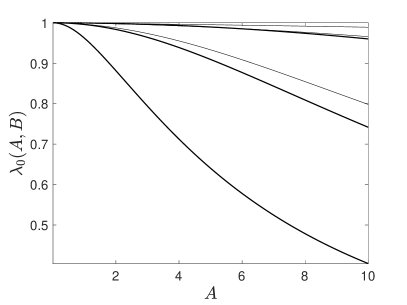
We now compute the positive principal eigenvalue to the quadratic linear eigenvalue problem for the Couette flow (8a) and the Poiseuille flow (8b) and use (50) with to evaluate in these two example cases. We use a standard second-order finite-difference discretization of (42)–(43). The resulting matrix eigenvalue problem is solved for a range of values of and using MATLAB’s routine polyeigs. We choose the spatial resolution to satisfy . The results are shown in Figure 1. It is clear that for these particular flows, the propagation speed is enhanced by advection, increasing with and decreasing with . Furthermore, for all values of and considered, the propagation speed in the Couette flow remains larger than in the plane Poiseuille flow.
We now proceed to consider (IBVP) or, equivalently (QIVP) and (BVP) or, equivalently (QBVP), in a number of significant asymptotic limits in the two key parameters .
3 Slowly varying front with strong advection: as
In this section we consider (IBVP) when the advection velocity scale is large compared to the advectionless front propagation speed, and the channel width is small relative to the advectionless front scale thickness. In terms of the two parameters and , we can formalise this by considering and , with the principal balances in the PDE (IBVPa) leading us to consider the limit , with as . For ease of notation, we write
| (53) |
with as . In what follows, to avoid issues with the discontinuity in the cut-off nonlinearity, it proves convenient to make use of an exact result, obtained via (IBVPa), (IBVPe) and regularity on , and given by,
| (54) | |||
Moreover, since the cut-off nonlinearity does not appear, at least up to order , we are able to work, to our advantage, directly with (IBVP), rather than the moving boundary formulation. We now introduce the expansion,
| (55) |
as , with . On substitution from (55) into (IBVP), we obtain, at leading order, the following problem for , namely,
| (56a) | |||
| which must be solved subject to | |||
| (56b) | |||
which requires,
| (57) |
with to be determined subject to suitable regularity, with
| (58) |
uniformly for , any , and
| (59) |
At in (IBVP) we obtain from (IBVPa)
| (60a) | |||
| which must be solved subject to | |||
| (60b) | |||
The solution to (60) is given by,
| (61) |
Here is to be determined, with suitable regularity, and
| (62) |
We observe from (62) that
| (63) |
so that, via (IBVPd). We now substitute from (55), (57), (61) and (62) into (54), and perform the integrations to obtain, at , the following PDE for , namely,
| (64a) | |||
| with | |||
| (64b) | |||
when is nontrivial. Equation (64a) must be solved subject to the initial and boundary conditions (59) and (58). With the scaling transformation . the initial value problem (64a), (59) and (58) for reduces precisely to that studied in detail recently in [24, 25]. In [24] it is established that the PDE (64) has a unique PTW solution with propagation speed
| (65) |
with as given in [24]. It should be noted that , the effective diffusivity introduced in subsection 1.1. The initial boundary value problem (64a), (59) and (58) is studied in detail in [25], where it is principally established that evolves into a PTW structure as . We are now able to interpret this for (IBVP) via (55). At leading order, as with , we observe that becomes rapidly homogeneous in (on a time scale as ) and thereafter is governed by the one-dimensional cut-off KPP reaction-diffusion equation (64a). The effect of the advective shear flow is simply to enhance the streamwise diffusion coefficient from unity to . For each , , a unique PTW exists, which has propagation speed,
| (66) |
as , with and as given in [24]. This PTW solution forms the large- attractor for (IBVP).
As reduces in order relative to , an examination of the PDE (IBVPa) reveals that the balancing of terms at undergoes a change, in particular when the distinguished limit becomes with . In this case we write
| (67) |
with, again, as . Returning to PDE (IBVPa), the natural scale in the coordinate is now of (so that the front thickness is increasing with ). Thus we introduce the coordinate , with
| (68) |
and the factor is for algebraic convenience. We next follow the earlier case, when , and expand as,
| (69) |
as with . Here now satisfies,
| (70) |
with suitable regularity, and again subject to initial and boundary conditions (59) and (58).The conclusions regarding (IBVP) and (BVP) are thus as for the case , except now the front is on the stretched length scale and (66) is modified to,
| (71) |
as , with . This completes the structure to (IBVP) and (BVP) in the case of slowly varying fronts, with and .
We end this section with comments on the behaviour of the PTW propagation speed. We observe from (66) and (71) that is enhanced by the shear flow through a prefactor that is entirely determined by the flow whilst the effects of reaction cut-off are felt through the factor corresponding to the propagation speed for the reaction cut-off problem in the absence of a flow. Thus, the asymptotic limits (2) and (3) are, in the presence of a shear flow, magnified by a factor entirely dependent on the flow. For , the enhancement is significant. Finally, simple calculations for the Couette and Poiseulle flows give, specifically,
| (72) |
Thus, the PTW propagates faster in the plane Couette flow than in the plane Poiseulle flow.
4 Slowly varying, balanced or rapidly varying front with weak advection: or as
In this section we consider (IBVP) ((QIVP)) and (BVP ((QBVP)) in the case when the advection velocity scale is small compared to advectionless front propagation speed, so that . To begin with we examine the structure to (IBVP) when also , so that the channel width is small compared to the advectionless front thickness. To formalise this case, we consider (IBVP) when as .
4.1 Slowly varying front: as
This limit considers the situation when the channel width is small compared to the thickness of the advectionless front. For notational convenience, we write
| (73) |
and then a balance in (QIVPa) determines an expansion in the form,
| (74) |
as with . Here, formally, as . On substituting from (74) into (IBVP), we obtain,
| (75) |
with to be determined, with suitable regularity. Moving to , we proceed as in section 3, and, without repeating details, we obtain the following scalar problem for , namely,
| (76) |
together with initial and boundary conditions (59) and (58). This is precisely the scalar evolution problem studied in detail in [24, 25], where it is established that evolves into a PTW structure as , and, for each , this PTW solution is unique, and has propagation speed , as given in [24]. Thus in this case, for (BVP),
| (77) |
as with . This simple case is now complete. To summarise this case, it follows from (75) that the deformation of the front interface is weak and of order whilst from (77) the correction to the propagation speed is even weaker. This correction can be considered via restricting attention to the problem (QBVP) since at higher order the detailed nature of the discontinuity in the reaction must be addressed and so, the free-boundary formulation (QBVP) needs to be adopted. We now move on to the next case.
4.2 Balanced front: as
This limit addresses the situation when the channel width is comparable to the front thickness in the absence of advection. In considering the limit as , since the discontinuity in the cut-off nonlinearity is encountered immediately, at leading order, it is most convenient to address the formulation (QIVP), and we restrict attention to PTW solutions to (QIVP), via the formulation (QBVP). We look for a solution to (QBVP) expanded in the form (with ),
| (78a) | |||
| as , with . In addition, for , we write, | |||
| (78b) | |||
| and expand the propagation speed, | |||
| (78c) | |||
We now substitute from (78) into (QBVP). Collecting terms at , we obtain the following problem for , and , namely,
| (79a) | |||
| with | |||
| (79b) | |||
| and | |||
| (79c) | |||
| uniformly for , whilst | |||
| (79d) | |||
| (79e) | |||
| (79f) | |||
| (79g) | |||
The elliptic problem (79) has a unique solution, and this solution is independent of . The solution is given in [24] (see Theorem 1) in terms of , namely,
| (80a) | |||
| with | |||
| (80b) | |||
| and | |||
| (80c) | |||
We recall, from [24], that is monotone decreasing in , with,
| (81a) | |||
| (81b) | |||
| (81c) | |||
| with the constant and | |||
| (81d) | |||
We now proceed to terms at in (QBVP). This results in the following inhomogeneous linear elliptic boundary value problem for , and , namely,
| (82a) | |||
| (82b) | |||
| (82c) | |||
| (82d) | |||
| (82e) | |||
| where (82d) and (82e) were obtained using (81a) and (81b). | |||
We first eliminate from the problem (82b)-(82e), which reduces the boundary conditions (82d) and (82e) to
| (83a) | |||
| (83b) |
for all , after which is given by
| (84) |
The linear elliptic problem (82) and (83) can be solved explicitly. We begin by using Fourier’s Theorem to write,
| (85) |
with () to be determined. We observe that the boundary conditions (82c) are satisfied by (85). In addition, we may write, via (QIVPj),
| (86a) | |||
| with | |||
| (86b) | |||
for . Now substitute from (85) and (86a) into (82a)–(82d), (83a) and (83b). At we obtain the following problem for ,
| (87a) | |||
| (87b) | |||
| (87c) | |||
| (87d) |
To solve (87), we first observe that is a solution to the homogeneous form of the linear ODE (87a). After writing this ODE in self-adjoint form, it is then readily established that the linear, inhomogeneous, boundary value problem (87a)–(87d) has the solvability condition
| (88) |
which requires
| (89) |
The solution to (87) is then given by,
| (90) |
with a constant to be determined. Now, from (33) and (78b), we require
| (91) |
which becomes, via (84),
| (92) |
| (93) |
Now , and so (90) and (93) requires , and therefore
| (94) |
For , we obtain the problem,
| (95a) | |||
| (95b) | |||
| (95c) | |||
| (95d) |
The solution to (95) is readily obtained as,
| (96) |
Thus, via (94) and (96), we have, from (85),
| (97) |
We recall that is given by (86), and so, it is convenient to introduce as,
| (98) |
Integrating (98) and rearranging yields
| (99) |
Thus we have,
| (100) |
Now, from (99), we obtain,
| (101) |
It is thus convenient to introduce
| (102) |
We can now use (101) and (102) to re-write (100) as,
| (103) |
with denoting the usual mean value on the interval . Finally, from (84) and (103), we obtain,
| (104) |
Thus, in this case we have, via (78), (80), (89), (94), (103) and (104),
| (105a) | |||
| (105b) | |||
| (105c) |
as with . We conclude in this case that there is a unique PTW solution, given by (105a) and (105b), for each , which has propagation speed,
| (106) |
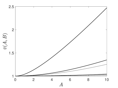
as with . We note that, although the correction to the PTW propagation speed is at least as small as , the corrections to the PTW structure are both at . We also note from (105b) with (102) and (98) that has interior stationary points if and only if has a zero in the interior of the domain. This completes the asymptotic analysis in the case with . Contrasting with the previous case, the correction to the propagation speed is of the same order when as , which is as expected. In fact we see that in both cases the correction to the propagation speed can be written, uniformly as as , and we will see that this continues to hold in each of the cases considered below in the rest of this section. We finally compute the interface deformation for the Couette flow (8a) and the Poiseuille flow (8b) using (105b) and (102). Figure 2 compares the deformation against the structure of the two flows. It is clear that the deformation in the Couette flow is more pronounced than in the plane Poiseulle flow.
The final case in this section is with , and the appropriate distinguished limit is as .
4.3 Rapidly varying front: as
Here we consider the asymptotic structure of PTW solutions when the front thickness in the absence of advection is small compared to the channel width. In this case, it is natural to consider PTW solutions via the formulation (BVP). Again, setting , we write,
| (107) |
with as . We now expand in the form,
| (108a) | |||
| (108b) | |||
| (108c) |
as . We substitute (107) and (108) into (BVP). At leading order we obtain the following problem for , and , namely,
| (109a) | |||
| (109b) | |||
| (109c) | |||
| (109d) | |||
| uniformly for , | |||
| (109e) | |||
| (109f) | |||
Since partial derivatives with respect to do not appear in the problem (109a)–(109d) we can address this problem following [24] and regard as a parameter. Thus, we may conclude that, up to translation invariance, (109) has a unique solution. Since we may regard the translational invariance as dependent on then we may write the solution as
| (110) |
| (111) |
with to be determined, so that , and satisfies condition (109f), together with,
| (112) |
via (110) with (109e). We next formulate the problem at from (BVP), which provides an inhomogeneous linear problem for and . After a significant amount of detailed, but routine, calculation on this problem (which, for brevity, we do not include here), we find that it requires a solvability condition arising from the classical Fredholm alternative which must be satisfied for the linear inhomogenous boundary value problem to have a solution. This provides a nonlinear eigenvalue problem which determines and , namely,
| (113) |
together with boundary conditions (112) and condition (109f), which we henceforth refer to as (EP). In considering (EP), we first introduce given by
| (114) |
which requires that
| (115) |
and, upon using (109f), that
| (116) |
In terms of this new dependent variable, (EP) becomes a classical regular Sturm-Liouville eigenvalue problem (see, for example, Coddington and Levinson [5]) that we will henceforth refer to as (SL):
| (SLa) | |||
| with boundary conditions | |||
| (SLb) | |||
| and condition where | |||
Indeed, (SL) has arisen via a very different route in the work of Haynes and Vanneste [14] in the context of a purely advection-diffusion problem at high Péclet number (corresponding to high ), and in relation to the present context, it has been studied by them for the particular Couette and plane Poiseuille flows noted in (8). The positivity requirement (115) dictates that we require the smallest (principal) eigenvalue of this Sturm-Liouville problem. We denote the principal eigenvalue by
| (117) |
and the associated principal, -normalised, eigenfunction by with
| (118) |
and
| (119) |
with the choice of normalisation being convenient at a later stage. The solution to (EP) is then given by, on satisfying the final condition (116),
| (120) |
with
| (121) |
We now consider (SL) in the two cases when and .
4.3.1 (SL) when
We consider (SL) as . An exposition of this type has been developed in [14], and for completeness we give a brief development in the present context. It follows from (SL) with (118) and (119) that
| (122) |
as . Thus we expand in the form,
| (123a) | |||
| (123b) |
as . On substitution into (SL) using (119), we obtain the problem
| (124a) | |||
| (124b) | |||
| (124c) |
The solution to (124) is readily obtained as
| (125a) | |||
| with given by (62), and, | |||
| (125b) | |||
Thus, via (120), (121), (123) and (125), we obtain,
| (126) |
| (127) |
as . It should be noted that these results, for , are in full accord with those of section 4.2, for . Expression (126) can be made more precise by performing higher-order corrections to , the details of which are presented in [14] and give
| (128) |
as . Upon using (121) these corrections yield
| (129) |
as .
4.3.2 (SL) when
We consider (SL) as . An analysis of this type has been given for the Couette and plane Poiseuille flow in [14]. Here we develop the theory to apply to any shear flow which has a continuous derivative on , and whose absolute maximum on occurs strictly at an interior point. First, let
| (130) |
when is nontrivial, via (IBVPd). Now, we restrict attention to the situation when is achieved () at a single point, which is in the interior of . We label this point as . Numerical experiments on (SL) with suggest that the principal eigenfunction, , under the normalisation (119), develops into a -sequence as , based at . This leads us to write
| (131) |
as , which automatically satisfies the normalisation (119). Now, upon integration and using (119), (SL) becomes
which gives, using (131), as . This suggests the principal eigenvalue of (SL) should be expanded as,
| (132) |
as , with to be determined. Using this, we may now determine the structure of as , in more detail, together with determining . We first anticipate, from (SL), that there will develop boundary layers at and , as . We focus attention first at . The boundary layer thickness will be , and so we introduce
| (133) |
as in the boundary layer. At leading order, (SL) becomes
| (134a) | |||
| (134b) |
The solution to (134) has,
| (135) |
as with , and a normalising factor to be determined. Similarly, for the boundary layer at , we introduce,
| (136) |
as in the boundary layer, after which we obtain,
| (137) |
as with , and a normalising factor to be determined. The remaining asymptotic structure now has three regions, as follows:
-
•
region :
-
•
region :
-
•
spike region : .
We first move to region . The form of solution (135) in the boundary layer at , leads to a WKB form for the solution in this region, which, after asymptotic matching with (135), gives,
| (138) |
as with . Similarly, in region we have,
| (139) |
as with . We finally move to the spike region. In this region we introduce
| (140) |
as . The expansions (138) and (139) require us to write
| (141) |
as with . Here as is to be determined. Substitution from (140), (141) and (132) into equation (SLa) gives, at leading order,
| (142a) | |||
| (142b) | |||
| whilst matching with region and region (via Van Dyke’s matching principle [27]) requires, on using (138) and (139), | |||
| (142c) | |||
and also that , and satisfy the two conditions,
| (143) |
| (144) |
In addition the normalising condition (119) requires,
| (145) |
In the above
| (146) |
restricting attention to a nondegenerate interior maximum for (the case when the interior maximum is degenerate can be similarly addressed). Now, (142a)-(142c) is a linear self-adjoint singular Sturm-Liouville eigenvalue problem on the whole real line. The positivity condition (142b) determines that must be the smallest (principal) eigenvalue. The condition (145) then normalises this eigenfunction. In fact, we can determine the lowest eigenvalue and the associated eigenfunction by inspection, which gives,
| (147a) | |||
| with, | |||
| (147b) | |||
It then follows, via (143)–(147a), that,
| (148a) | |||
| (148b) | |||
| (148c) |
Finally, via (132) and (147b), we have,
| (149) |
as , and so (121) gives,
| (150) |
as . The analysis in this subcase is now complete. However, it is instructive to note that the structure will be adjusted when or as , and in particular, when or as . A detailed consideration of the case when as , reveals that the leading order form of remains unchanged, but the correction is influenced, so that, in these cases,
| (151) |
as . Evidently, the case of Couette flow falls into this category, and the details for this case are developed in [14], where it is established that the above correction is, in fact, of . For brevity we do not pursue these special cases further.
4.3.3 (SL) when
In this case, details of (SL) must be obtained numerically. However, since we are dealing with the principal eigenvalue, whose normalised eigenfunction is strictly positive, a simple integration of equation (SLa) over the interval , using conditions (SLb), and rearranging, establishes the following bounds on , namely
| (152) |
for all , with
| (153) |
when is nontrivial. We can thus conclude, from (121), that,
| (154) |
for all . In fact, we can improve the upper bound on , by again using the strict positivity of the principal eigenfunction to establish, after dividing through equation (SLa) by and, using integration by parts together with (IBVPd), that
| (155) |
for each , when is nontrivial, and so we then have the improved lower bound
| (156) |
for all .
It is instructive at this stage to summarise the asymptotic results concerning PTW solutions as , the case of weak advection. We have considered the situation when , and , in the natural distinguished limits, as . We have shown that, when , then for each , there exists a unique PTW solution to (BVP) (correspondingly (QBVP)), with propagation speed denoted by . With regards to this propagation speed, we have determined that, as ,
-
(i)
or
(157) -
(ii)
()
(158) Here
(159) and is the principal eigenvalue of the Sturm-Liouville problem (SL). We have established, upon use of results in [14], that when (so that ), then,
(160) whilst when (so that ) then,
(161)
We observe that the effects of weak advection on the PTW propagation speed is always of as , but becomes more significant with decreasing . It is also worth noting here that expansion (158) forms a composite expansion for as for all , with error uniformly of . In addition, it follows from this observation and the limiting forms (160) and (161), that the correction to the propagation speed is of when , initially decreasing from the value as , and continuing to decrease with increasing , becoming of for , and decreasing at a rate of . We finally observe that the two complimentary asymptotic forms for the propagation speed as , given in (157) and (158) match with each other according to Van Dyke’s asymptotic matching principle [27]. To conclude this section, we now compare the moving boundary location in the PTW solutions. Assembling the results of this section we obtain, as , that the moving boundary is at spatial location for , with,
-
(i)
(162) -
(ii)
(163a) with (163b) -
(iii)
()
(164) with . Here is the principal, -normalised eigenfunction of (SL). The structure of as () and as () is as given in subsections 4.3.1 and 4.3.2.
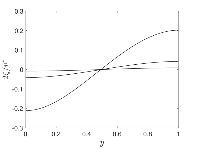
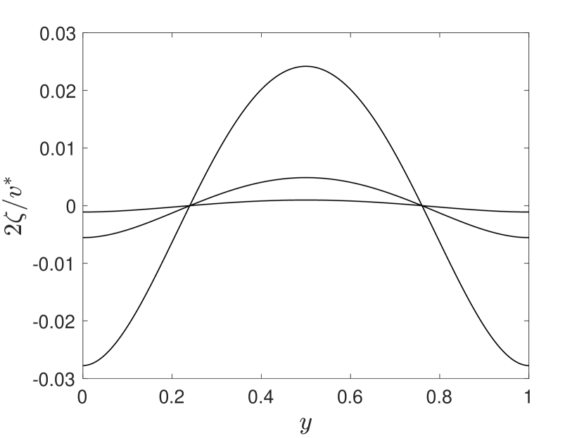
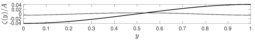
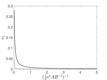
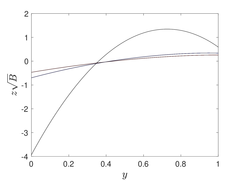
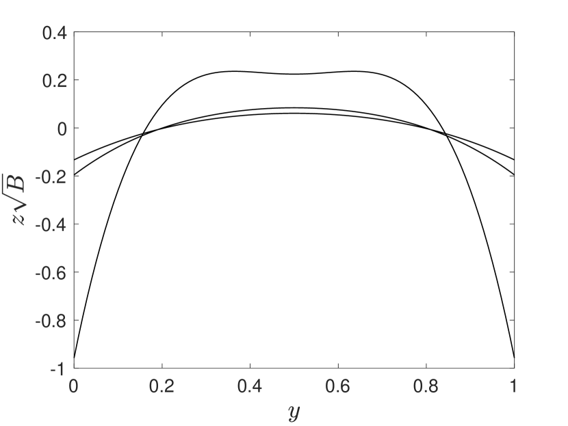
Figure 3 shows the correction to speed of propagation of the PTW solution (divided by ) computed by numerical solution of the (SL) eigenvalue problem for the Couette and Poiseuille (8) flows. Clearly, the enhancement to the speed is, for fixed (small) , greater for the Couette flow than for the Poiseuille flow, decreasing monotonically as either the front thickness or cut-off value increase. Figure 4 shows the leading order scaled interface , deduced from (120) for three different values of . The interface becomes increasingly flat as either the front thickness or cut-off value increase.
We now move on to consider PTW solutions when advection and streamwise diffusion are balanced.
5 Slowly varying or rapidly varying front with balanced advection: or with
In this section we consider (IBVP) ((QIVP)) and (BVP) ((QBVP)) in the final case when the advective fluid velocity is comparable to the advectionless front propagation speed, so that . We consider this situation first when the channel width is small compared to the advectionless front thickness (), and then when the channel width is large compared to the advectionless front thickness (). We begin with the former case.
5.1 Slowly varying front:
Following details very similar to those presented in section 3 (and without repetition) we have, for (IBVP),
| (165) |
as , with , where satisfies the one-dimensional evolution problem comprising the PDE (64a), with , subject to the initial and boundary conditions (58) and (59). It then follows, regarding PTW solutions, that the propagation speed has
| (166) |
as with . With the PTW moving boundary at , it also follows from (165) that,
| (167) |
as with .
5.2 Rapidly varying front:
We restrict attention to PTW solutions, and the most convenient formulation to work with is that given in (BVP). It is convenient to write
| (168) |
The form of the PDE (BVPa) with as , leads us to write,
| (169) |
as with , and , each having , , as . In addition we require,
| (170) |
via (BVPe). In addition to (169) we also expand,
| (171) |
as . On substitution from (169) and (171) into (BVP) we obtain, at leading order,
| (172) |
with ′ representing differentiation in the respective arguement, and where , replacing , is given by,
| (173) |
Since and are independent coordinates, the solubility of (172) requires, without loss of generality,
| (174a) | |||
| (174b) | |||
| for , on normalising so that, | |||
| (174c) | |||
| The boundary conditions in (BVP) require, | |||
| (174d) | |||
Before considering (174) in more detail, we first write down the problem for , which becomes, via (174), and (170),
| (175a) | |||
| subject to | |||
| (175b) | |||
| (175c) | |||
This problem has the solution (as noted in previous sections, and see also [24]),
| (176) |
and we recall from [24] that,
| (177) |
Now, following (169) and (176), the moving boundary, where , occurs at , and so, via (171), when
| (178) |
and so, we must have, via (BVP) ((30)),
| (179) |
To proceed we will limit attention to shear flows which have a single point of maximum velocity , occuring at , where, without loss of generality, we may take . Next we observe from (174b) that the continuous functions and achieve their maximum values on , of unity and respectively, at the same point , after which (174b) evaluated at , requires,
| (180) |
Equation (174b) then becomes
| (181) |
We are left with (172) to determine . We also note that, in general, (181) will not satisfy the boundary conditions in (174d), and passive boundary layers will be needed, when and . For brevity, we do not consider these boundary layers here. We observe from (181) that,
| (182) |
as specified in the normalisation (174c). In addition the stationary points of and are coincident. Now, equation (174a) can be re-written as
| (183) |
Therefore,
| (184) |
so that an integration gives,
| (185) |
with the constant determined by the condition (179). We note that, as required, , with passive boundary layers required when over which the boundary conditions (174d) will be satisfied. In summary we have, in this case of balanced advection, with the channel width large compared to the streamwise diffusion length scale (based on the reaction time scale), a PTW solution for each , with propagation speed
| (186) |
as with . In addition, the moving boundary has location,
| (187) |
as with , given by (185) and given by (174b). We now compute the interface deformation for the Poiseuille flow (8b) by numerically integrating (185) with (179) for three different values of corresponding to small, intermediate and large cut-off . As the cut-off increases, the maximum of the interface and its deformation increases.
6 Conclusions
In this paper we have considered a reaction-diffusion process evolving inside an infinite channel in the presence of a shear flow. The reaction function is of standard KPP-type, but experiences a cut-off in the reaction rate below the normalised cut-off concentration . We have formulated this initial-value boundary problem (IBVP) in terms of an equivalent moving boundary evolution problem (QIVP) and examined both of these problems in a number of natural asymptotic limits relating to the two non-dimensional (positive) parameters and describing the strength of the flow and front thickness, whilst keeping fixed. We have established in all cases considered, that a unique (up to spatial translation) PTW solution exists, and in a number of cases, that this forms a large- attractor for (IBVP). We used the method of matched asymptotic expansions to determine the detailed structure of the PTW solutions and their speed of propagation and, in particular, their dependence on the parameters. It is of interest to examine the nature of the propagation speed in the three complementary regimes , and over the full range of . Using the results captured by Figure 3, is fully determined, up to the stated orders in , as a function of as . Partial results obtained in the other two regimes are completed by extracting and extrapolating limiting forms of the available asymptotic expressions. We therefore expect that for and , the speed of propagation decreases monotonically with . We anticipate that the approach developed in this paper will be readily adaptable to the case of two corresponding problems, when the KPP-type cut-off reaction function is replaced by a broader class of cut-off reaction functions or when the shear flow is unsteady, varying periodically with time. Finally, it would be interesting to determine whether similar qualitative effects arise for a certain stochastically perturbed KPP equation obtained from an alternative model whose purpose is also to account for microscopic discrete particles [6, 7]. Mueller, Mytnik and Quastel [20] have shown that in the absence of a shear, the difference between the speed obtained from this model and obtained from the deterministic cut-off model considered here is small when the cut-off and noise are both small. Whether this difference continues to be small in the presence of a shear flow is presently unknown.
Acknowledgments. The authors acknowledge A. D. O. Tisbury for his early contribution on this project. We also thank the referees for their constructive comments, which have led to an overall improvement in the presentation of the paper.
Appendix A Asymptotic solution to (QIVP) as
As the nature of the discontinuity in the initial condition of (QIVP) and the requirement for this to be locally spatially smoothed in the small time limit, demands a diffusion balance at leading order in (QIVP). As a consequence of this, it follows that the solution to (QIVP) develops in four principal asymptotic regions, which are,
-
•
Region : , with as
-
•
Region : , with as
-
•
Region : , with as
-
•
Region : , with as
with, in addition,
| (188) |
A similar structure characterises the case in the absence of advection and this is developed in [25], where a qualitative sketch of the above regions is also included. Throughout denotes being positive or negative, respectively. A balance of terms in the PDE (QIVPa) indicates that, with regions having as , then,
as . Thus we expand in the form,
| (189) |
as , with . The details in regions are straightforward, obtained by introducing the coordinate and in both regions expanding
| (190) |
Substituting expansions (189), and (190) into the equation for we obtain that and satisfies
| (191a) | |||
| subject to | |||
| (191b) | |||
| together with matching conditions with regions IIL and IIR which requires, | |||
| (191c) | |||
It is straightforward to determine
| (192) |
for . At the next order, we obtain that satisfies
| (193a) | |||
| subject to | |||
| (193b) | |||
| with , together with matching conditions with regions IIL and IIR which requires, | |||
| (193c) | |||
Solving (193) yields
| (194) |
for . Thus, we have via (192) and (194) that
| (195a) | |||
| as , uniformly for , with | |||
| (195b) | |||
| and | |||
| (195c) | |||
| uniformly for as . | |||
An interesting interpretation of these asymptotic forms is that gives the diffusive displacement, whilst gives the advective displacement, respectively, of the spatial moving boundary in the early times. However, reaction plays no role, up to .
We now move on to regions . It follows from (195a) that and are exponentially small in as in regions and , respectively. The details are lengthy, but standard (see, for example, [25] for more details for the case when for ), and are omitted for brevity. After matching with regions and respectively, we have
| (196) |
with being the usual Heaviside function, and
| (197) |
as , with .
At this stage the asymptotic structure as is not quite complete. In obtaining the expansions in regions and , we have been forced to neglect the Neumann boundary conditions at and , and an examination of these expansions reveals that,
| (198) |
when in regions as , whilst,
| (199) |
when in regions as . Thus, weak and passive boundary layers are required when and as , adjacent to both regions and . These boundary layers are readily dealt with, and since they are passive in nature, for brevity we do not present details here. This completes the asymptotic structure of the solution to (QIVP) as .
References
- [1] H. Berestycki, The influence of advection on the propagation of fronts in reaction-diffusion equations, in Nonlinear PDEs in Condensed Matter and Reactive Flows, H. Berestycki and Y. Pomeau, eds., vol. 569 of NATO Science Series C, Kluwer, Doordrecht, 2003.
- [2] H. Berestycki and L. Nirenberg, Travelling fronts in cyclinders, Ann. I. H. Poincaré, 9 (1992), pp. 497–572.
- [3] E. Brunet and B. Derrida, Shift in the velocity of a front due to a cut-off, Phys. Rev. E., 56 (1997), pp. 2597 – 2604.
- [4] R. Camassa, Z. Lin, and R. M. McLaughlin, The exact evolution of the scalar variance in pipe and channel flow, Commun. Math. Sci., 8 (2010), pp. 601–626.
- [5] E. A. Coddington and N. Levinson, Theory of ordinary differential equations, McGraw-Hill, New York, 1955.
- [6] J. C. Conlon and C. D. Doering, On travelling waves for the stochastic Fisher-Kolmogorov-Petrovskii-Piscounov equation, 120 (2005), pp. 421–477.
- [7] C. R. Doering and F. Tesser, Discrete and Continuum Dynamics of Reacting and Interacting Individuals. In: Muntean A., Toschi F. (eds) Collective Dynamics from Bacteria to Crowds. CISM International Centre for Mechanical Sciences, vol. 553, Springer, Vienna, 2014.
- [8] F. Dumortier, N. Popovic, and T. J. Kaper, The critical wave speed for the Fisher-Kolmogorov-Petrovskii-Piscounov equation with cut-off, Nonlinearity, 20 (2007), pp. 855–877.
- [9] D. Gilbarg, and N. S. Trudinger, Elliptic Partial Differential Equations of Second Order, Berlin-Heidelberg-New York-Tokyo, Springer-Verlag (1983).
- [10] P. F. Embid, A. J. Majda, and P. E. Souganidis, Comparison of turbulent flame speeds from complete averaging and the G‐equation, Phys. Fluids, 7 (1997), pp. 2052–2060.
- [11] R. A. Fisher, The wave of advance of advantageous genes, Ann. Eugenics, 7 (1937), pp. 355–369.
- [12] M. I. Freidlin, Functional Integration and Partial Differential Equations, Princeton University Press, 1985.
- [13] J. Gärtner and M. I. Freidlin, On the propagation of concentration waves in periodic and random media., Soviet Math. Dokl., 20 (1979), pp. 1282–1286.
- [14] P. H. Haynes and J. Vanneste, Dispersion in the large-deviation regime. Part 1: shear flows and periodic flows, J. Fluid Mech., 745 (2014), pp. 321–350.
- [15] A. N. Kolmogorov, I. G. Petrovsky, and N. S. Piskunov, Étude de l’équation de la diffusion avec croissance de la quantité de matière et son application à un problème biologique, Bull. Univ. Moskov. Ser. Internat. Sect., 1 (1937), pp. 1–25.
- [16] A. J. Majda and P. R. Kramer, Simplified models for turbulent diffusion: Theory, numerical modelling, and physical phenomena, Phys. Rep., 314 (1999), pp. 237 – 574.
- [17] A. J. Majda and O. E. Sougadinis, Large-scale front dynamics for turbulent reaction–diffusion equations with separated velocity scales, Nonlinearity, 7 (1993), pp. 1–30.
- [18] J.-F. Mallordy and J.-M. Roquejoffre, A parabolic equation of the KPP type in higher dimensions, SIAM J. Math. Anal., 26 (1995), pp. 1–20.
- [19] P. D. Miller, Applied Asymptotic Analysis, Volume 75 of Graduate studies in Mathematics, American Mathematical Society, Providence RI, 2006.
- [20] C. Mueller, L. Mytnik, and J. Quastel, Effect of noise on front propagation in reaction-diffusion equations of KPP type, Invent. Math., 184 (2011), pp. 405–453.
- [21] G. Papanicolaou and J. Xin, Reaction-diffusion fronts in periodically layered media, J. Stat. Phys., (1991), pp. 915–931.
- [22] J. M. Roquejoffre, Eventual monotonicity and convergence to travelling fronts for the solutions of parabolic equations in cylinders, Ann. I. H. Poincaré, 14 (1997), pp. 499–552.
- [23] A. Stevens, G. Papanicolaou, and S. Heinze, Variational principles for propagation speeds in inhomogeneous media, SIAM J. Appl. Math., 62 (2001), pp. 129–148.
- [24] A. D. O. Tisbury, D. J. Needham, and A. Tzella, The evolution of traveling waves in a KPP reaction-diffusion model with cut-off reaction rate. I. Permanent form traveling waves, Stud. in App. Math., 146 (2021), pp. 301–329.
- [25] , The evolution of traveling waves in a KPP reaction–diffusion model with cut-off reaction rate. II. Evolution of traveling waves, Stud. in App. Math., 146 (2021), pp. 330–370.
- [26] A. Tzella and J. Vanneste, Chemical front propagation in periodic flows: FKPP versus G, SIAM J. Appl. Math., 79 (2019), pp. 131–152.
- [27] M. Van Dyke, Perturbation Methods in Fluid Mechanics, Parabolic Press, 1975.
- [28] J. Xin, Front propagation in heterogeneous media, SIAM Rev., 42 (2000), pp. 161–230.
- [29] J. Xin and Y. Yu, Sharp asymptotic growth laws of turbulent flame speeds in cellular flows by inviscid Hamilton–Jacobi models, Ann. I. H. Poincaré AN, 30 (2013), pp. 1049 – 1068.