Listen and Move: Improving GANs Coherency in Agnostic Sound-to-Video Generation
Abstract
Deep generative models have demonstrated the ability to create realistic audiovisual content, sometimes driven by domains of different nature. However, smooth temporal dynamics in video generation is a challenging problem. This work focuses on generic sound-to-video generation and proposes three main features to enhance both image quality and temporal coherency in generative adversarial models: a triple sound routing scheme, a multi-scale residual and dilated recurrent network for extended sound analysis, and a novel recurrent and directional convolutional layer for video prediction. Each of the proposed features improves, in both quality and coherency, the baseline neural architecture typically used in the SoTA, with the video prediction layer providing an extra temporal refinement.
1 Introduction
The invention of Generative Adversarial Networks (GANs) [23] and later convolutional GANs [51] has enabled the synthesis of a large and realistic variety of images. By confronting two networks, the generator and discriminator are able to implicitly learn complex data distributions. Shortly thereafter, conditional GANs devised new modulation mechanisms to have more control over the adversarial synthesis, by either conditional embeddings [52, 74] or explicit conditional images [29].
The emergence of conditionals GANs resulted in a diversity of cross-modal synthesis by mapping data between different domains. For that, a semantic link must exist between both source and target domain, i.e. their probability distributions must not be independent. Some examples are text-to-image [74, 70, 80, 42, 73], text-to-video [48, 60, 2, 16, 34, 26], speech-to-face [63, 11], video-to-sound [41, 78, 13, 9], or video-to-video[66].
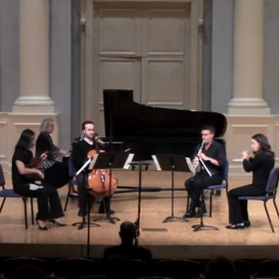
This paper focuses on generic sound-to-video translation. This entails a highly unconstrained problem, more than other modalities, because the physically plausible motion of objects has to be estimated exclusively according to the semantics of the produced sound. Certainly, multiple visual variations are plausible for a single sound. Moreover, video synthesis must deal with pixel jittering and audio-visual lagging, which is irrelevant for still images and to which human perception is extremely sensitive. In contrast to other modalities, such as speech-to-face, no prior distribution is assumed for either image or sound. Compared to pose-based approaches, this could tackle situations in which the human pose is difficult to infer, such as a face profile, occluding objects, or even an entire music ensemble performance. In a more general sense, it enables applications such as music-guided video restoration, audiovisual performance reinterpretation, agnostic speech replacement, or audio-reactive video animations.
2 Related works
In recent years, the ability of GANs to translate from audio to image has been demonstrated [12, 27, 64, 71, 18], yet frames are independently synthesized without temporal coherency. A common practice to leverage GANs from image to video is to use some sort of 3D video discriminator [53, 41, 57, 60, 2, 16, 77, 34, 57, 11, 63]. Although this should ideally be sufficient, an image discriminator on its simpler layout improves the convergence in adversarial training, providing feedback for both image quality and temporal dynamics [60].
Another common approach to induce temporal coherency consists in feeding the generator with a series of noise vectors temporally encoded by a Recurrent Neural Network (RNN). Intuitively, the RNN maps a sequence of feedforward independent random variables to a sequence of correlated random variables, representing temporal dynamics along the video stream.
In particular, MoCoGAN [60] —recently extended in [56]— proposed a novel framework for unconditional video generation disentangling motion from content by feeding the generator with an additional source of noise. The authors showed a decomposed representation was able to fabricate more coherent videos. Although it was not particularly adopted by other subsequent works, it is adapted in this work for audio conditioning.
Alternatively, MoCoGAN-HD [59] presented a particular feedforward scheme to map motion trajectories in a latent space pre-trained for still images, which ultimately fails to represent fine-grained temporal dynamics. Similarly, a text-driven sound-to-video method has been proposed in [39].
Furthermore, Dilated RNNs have been used for raw audio generation [62] and data series processing [7, 76]. However, dilated schemes has been omitted for GANs video generation hitherto.
In parallel, some optimizations have been proposed in speech-driven video synthesis, specially tailored for facial attributes, involving mouth generation [10, 57], lip reading [57], encoded action units [50, 49], or facial landmarks [11], a word-based learning for lip-facial attribute disentangling [77], or a third discriminator for audio-visual synchronization [63]. Most of these approaches use a reference frame, which reduces image uncertainty but ultimately produces rigid, unnatural movements. Other approaches have exploited body landmarks to assist in music-driven video performances [79]. However, albeit significant, these methods cannot be applied in its entirety for generic (faceless or bodyless) sound-to-video synthesis.
To induce temporal coherency at video level, vid2vid [66] relies on pre-trained flow models and previously synthesized frame feedback. Such an approach however is simply not feasible for sound-to-video. Fortunately, the apparition of ConvRNNs [55, 58] has enabled an efficient spatial analysis and temporal coherence by replacing with convolutions the gated matrix multiplications inside the recurrent cell. Vanilla ConvRNNs have proven to be more efficient than flow-based solutions for video prediction in non-causal configurations [5]. They have also been used for video encoding [3] and video representations [43], as well as landmark-based video synthesis from speech [11] or music [79]. Inspired by [5] to enhance temporal coherency, a novel directional and causal ConvGRU for video prediction is proposed in this work.
In addition, increasing image quality and resolution is particularly challenging in GANs. The stability of the adversarial training is usually affected as resolution scales. While most domain translation approaches use a two-stage architecture [74, 67, 71, 18], an improved StyleGAN [33] has evidenced the benefit of either residual or skip connections. Other methods have proposed different convolutional optimizations [31, 54]. Still, the task of generating smooth high-quality videos is a challenging problem [1, 53, 60, 72, 54, 59]. The caveat, as shown later, is that sound-driven learning has its own particularities to scale up.
Finally, it is worth mentioning methods based on attentional architectures (VQGAN) for sound-to-video [22, 8, 38], which however usually operate at low resolution and reveal collapsed examples. Beyond GANs, AD-NeRFs [25] showed outstanding speech-to-video synthesis, but based on a facial-tailored solution separately modeling various bust parts.
Contributions. The aim of this work is to improve both image quality and temporal coherency of generic sound-to-video GANs through three main novelties:
-
•
A more versatile triple sound routing for motion encoding, content representation, and conditional normalization layers.
-
•
A residual multi-scale DilatedRNN for an extended audio analysis and listening range.
-
•
A multi-orientation causal video prediction layer built upon a novel Directional ConvGRU.
3 Main architecture
The proposed model is made of four main neural networks, as illustrated in Fig. 1. A recurrent neural network models the physically plausible motion paths over time. Next, a generator maps audio-guided motion tokens into video sequences, as close as possible to real distributions. Then, the realism of ’s outputs is compared to real training samples by a couple of discriminators. Thus, focuses on individual images, while on the notion of motion by criticizing video sequences.
3.1 Sound representation
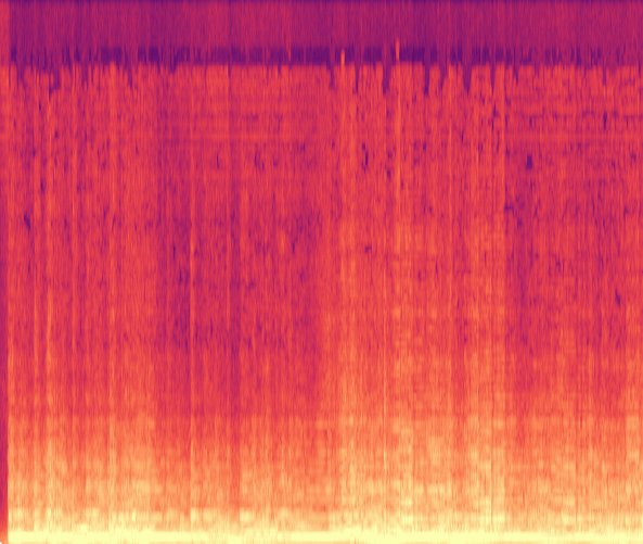
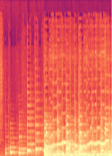
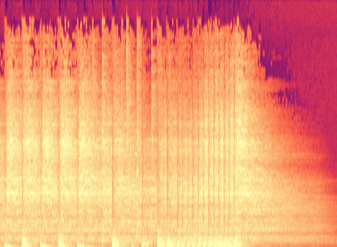
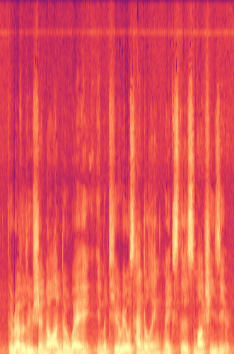
Extracting features from sound is a fundamental piece in the whole pipeline. Spectrogram representation is a common technique in single audio domain GANs [17, 36, 46] and is closely related to human hearing. In practice, the spectrogram is computed applying on a sliding window series the Short-Time Fourier Transform (STFT), to which the Log Mel Spectrogram (LMS) is a commonly applied perceptual non-linearity [12, 27, 18, 39].
Previous music-to-image methods, above mentioned, use spectrograms in their original bidimensional shape through a symmetric UNet-like generator. However, such an approach is too rigid and unnecessarily symmetric to scale up towards higher resolutions. On the other hand, the speech-to-video methods tend to draw upon more flexible representations.
Let denote a spectrogram of frequency bands, split in chunks from a -index sliding window of audio frames (time bins) and stride . Then, the sound features of each audio chunk can be defined as . The waveform is effectively converted into log mel frequency bins (filtering frequencies -) with a window length and hop size.
The duration of the audio chunks, i.e. the temporal resolution, is critical. Human perception is highly sensitive to periodic waveforms —such as speech or music— in short to medium timescales (-) [19]. In speech recognition fine-grained intervals, such as -, are often used [45], while the average phoneme duration for instance in English might be around [15]. From a music perspective, - corresponds to sixteenth-notes (\musSixteenth) at - beats per minute, which is a reasonable upper bound. We finally set an intermediate value of (). The effective temporal resolution will eventually be constrained by the video frame rate, whose inverse is the hop size, hereafter fixed to () or . Note that chunk overlapping —in this case — already encourages temporal coherency. Herein, the first video frame is taken for each audio chunk.
3.2 Audio temporal coherency
A basic yet effective way of inducing temporal correlation is by means of RNNs, which also helps to generate videos of varying length even beyond the training length [2]. Indeed, an auxiliary generator has better efficiency than a 3D generator alone [53], which struggles to generate coherent sequences beyond the training length, as corroborated here in preliminary experiments.
Among the RNN family, Gated Recurrent Unit (GRU) and Long Short-Term Memory (LSTM) are used indistinctly. In fact both perform comparable for speech and music analysis [14]. Here, the former is favored given its more efficient memory and computation requirements.
At this point, an important design choice resides in source of motion and sound routing, see Fig. 1. These types of routing are not either mutually exclusive or redundant, in fact their combination is beneficial, as shown later. Hereafter, let denote a -enrolled and compact motion encoding of size performed by an RNN.
Sound as content. A precursor MoCoGAN disentangles content from motion by feeding the generator with two independent noise vectors. One represents frames as points in the latent space and the other encodes a latent motion path between frames. Thus, is a -length sequence of random vectors of normal distribution , where typically . Here, content noise is replaced by sound features , so that the generator’s input is concatenated channel-wise across the temporal dimension as , with . An important strength of this approach is that the generator has direct access to the raw sound features at each time step.
Motion from sound. In this approach the sound features are passed through the recurrent network, sometimes concatenated with motion noise as of size , so that the generator simply receives . This is a preferred configuration of most audio-driven video generation methods [57, 63, 57, 11, 40, 2, 39]. Albeit it entails a much harder task, since motion associated with elementary sound events —notes or phonemes— and their transitions needs to be encoded by a simpler recurrent network.
Dilated and residual recurrency. A multi-layer RNN with dilated skip connections is proposed to deal with more complex temporal dynamics of sound, which sometimes unfolds at different resolution speeds. Also, residual connections are routed to facilitate the propagation of audio features through the network, see Fig. 2. To formalize that, let’s reformulate the recurrent encoding as:
| (1) |
where is the output at time step of the recurrent cell at layer , which receives the previous layer’s output and the skipped hidden state with dilation factor . stands for an activation function, e.g. LeakyReLU. For instance, with the settings in Sec. 3.1, stacked layers result in , , and audio hops.
Single sequence batch size. A key architectural aspect herein falls to batch size and overfitting a single video. Most implementations reset the RNN’s init state after each training iteration, either with zeroes or a random vector. By doing this, multiple video sequences can be batched in a single training pass. Indeed, large batches are beneficial also for GANs [4]. Nevertheless, we observed that the unrolling of temporally ordered batches of size 1 with consecutive video sequences was critical for convergence, so the last internal state becomes the initial state of the following batch.
3.3 The adversarial networks
The generator and both discriminators are built upon a series of feedforward layers, made of convolutional, normalization, and activation layers, see Fig. 3. While the discriminators use batch normalization, the generator uses audio conditional instance normalization and noise injection [20, 32].
Sampling layers before every convolutional layer performed best in this work. Although most implementations prefer a kernel size 4 and sampling stride 2 [29, 4, 32], a symmetric configuration with kernel size 3 and stride 1 was utilized. Either way, the output resolution doubles as the network progresses to the outermost layers. Nearest-neighbor interpolation is used for up-sampling, while 2D-3D average pooling is used for down-sampling.
The number of channels doubles as each network progresses to the innermost layers, noted generically as for simplicity. Convolutional layers with kernel size 1 are used to convert between a -channel latent and 3-channel color spaces, supplemented with gates.
To scale-up the network towards high-resolution regimes, different configurations from [33] were tested in Sec. 5.2, using residual and skip connections respectively for and s.
Audio conditional generator. A format layer first replicates both spatial dimensions to accommodate the input vector into the first generative layer, until reaching dimensionality . Then a convolutional layer outputs latent vectors. Thus, the output video size relates to the number of layers as . Note that a batch of 1 sequence is unrolled and the generator effectively receives frames per training iteration.
In order to reinforce access to conditional data traveling through the generator, a well-known strategy consists in embedding class vectors modulating normalization layers [32, 4], which is seemingly exploited also in conditional video generation [59, 56, 39], while others prefer disentangled generative layers [68]. Here, as illustrated in Fig. 3(a), each sound feature vector , intuitively related to a set of related visual poses or layouts, is encoded into a class feature vector, ultimately modulating a conditional instance normalization layer. This can be formalized for each generative layer as:
| (2) | |||
where and are the mean and variance across spatial dimensions of the actual input activations . The matrices , are weights and , biases of each learnable linear transformation. is an activation function, e.g. LeakyReLU.
Image and video discriminators. Both and have the same number of layers as . At their output a decision layer embeds channels into by means of convolutions as PatchGAN to encourage discrimination in local patches and potentially improve high-frequency details [29, 50, 60, 18].
is built on 3D kernels, one temporal and two spatial dimensions equally sampled at the beginning of each layer, see Fig. 3(a). Note the temporal dimension can be downsampled times, e.g. sequences allow for temporal reduction only along the first layers.
For each forward pass receives a random frame from a synthetic video sequence . The same random index is used to pick up a real frame from a source sequence . Presumably, by sharing the same index, the mapping between sound features and visual attributes is facilitated. receives real and fake video sequences, as well as a shuffled version to reinforce temporal coherency [2].
3.4 Video temporal coherency
A novel recurrent multi-directional convolutional layout is proposed for causal video prediction. The activation distribution at time step can be expressed as , where are the hallucinated output activations of a generative layer and directional predictions. To do so, a video prediction layer is formed by 4-directional ConvGRUs (DirConvGRU), predicting positive and negative motion in horizontal and vertical directions, as well as a squared-centered ConvGRU, dealing with motion along the camera axis. See Fig. 4.
An amenable implementation is built under the assumption that opposite directions can share weights [5] and directionality can be achieved by aggregating increasingly larger and shifted one-dimensional kernels.
Let be a -shifted kernel predicting negative horizontal movements, and a negative horizontal translation operator, such that . By the translational equivariance property of convolutions it is straightforward that , where is the centered version of . Similar reasoning can be done for the equivalent horizontal and vertical , kernels. Thus, directional kernels of triangular shape inside DirConvGRUs are now easily constructed by adding up activations of multiple -shifted kernels of increasing size and shared bias. Furthermore, this allows to implement weight sharing between opposite directions by utilizing the same DirConvGRU layer, whose kernels’ outputs are properly shifted according to the desired direction.
The video prediction layer is stacked after the outermost generative layer, although it can be potentially inserted in each of the generative layers. The video prediction activations are finally concatenated as:
| (3) |
where is the -th hidden state, also output, of a -size centered or directional ConvGRU for .
The next step deploys a combination strategy. A weighted blending layer not only merges all directional predictions [5] but also predicts an auto-regressed attention mask [50, 11, 66, 6], which helps to merge both the hallucinated and predicted pixels as follows:
| (4) | |||
where the blending and masking weights are implemented as -channel convolutions ( for convenience). The activation functions and are sigmoid and the identity respectively —LeakyReLU performed slightly worse. Also, denotes the channel-wise Hadamard product, and is the hallucinated output with induced temporal coherency.
4 Training and loss function
The importance of the loss function has sometimes been questioned [44, 37]. Nevertheless, no other apart from Wasserstein with gradient penalty (WGAN-GP) [24] was able to provide training stability and image quality in this work. In addition, perceptual loss [30] has shown a remarkable capability to synthesize sharper details [57, 10, 66, 67, 6, 79, 59]. In a preliminary study, it obtained about dB better accuracy, about faster convergence, and notably more stable training compared to the -norm.
Let represent a ground truth video sequence, paired for each audio chunk with its sound representation , as described in Sec. 3.1. Likewise, a synthesized video sequence is implicitly defined as . Then, the minimax adversarial loss function, expressed in two terms , is defined as:
| (5) |
| (6) | |||
where each discriminator’s gradient penalty is expressed as , related to source , modeled , and shuffled video data distributions. Individual image distributions are subscripted. The perceptual loss uses to denote the output features of an intermediate VGG layer. Hyper-parameters and are meant to control the importance of loss terms during training. For every training iteration, alternating gradient updates are conducted. First and are updated while fixing and , and vice versa.
5 Experiments
Training on a single video might give the impression of being an easy-to-learn task. However, other normalization types and loss functions led to divergence or model collapse. Moreover, successful setups needed about a training day ( iterations) for and about 3 days ( iterations) for to reach a decent image quality111Intel(R) Core(TM) i9-10900X CPU @ 3.70GHz and NVIDIA GeForce RTX 3090.. Full-model higher resolutions required far beyond GPU-memory and too long training runs that were finally discarded.
5.1 Hyper-parameters setup
Batched video sequences have frames forwarded one at a time. The size of random noise vectors is (just a guess). The input and hidden recurrent layers have the same size , so eventually the generator ingests vectors of size . Image resolution is achieved with generative layers. The outermost one has channels, incremented in powers of two, with maximum channels. Images are normalized. uses normal initialization and zeroed init states (no prior). Convolutional weights receive a random initialization from a normal distribution , while DirConvGRUs use orthogonal initialization. All LeakyReLUs have negative slope. TTUR learning rates are heuristically set to for and , while and updates at , without scheduling. The Adam optimizers [35] have momentums of and , with .
5.2 Model assessment
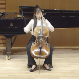
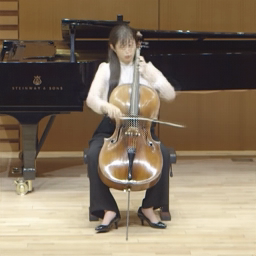
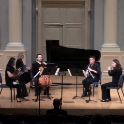
The goal of this work is to improve GANs ability to regenerate videos based exclusively on its audio as guidance, as realistic and coherent as possible, to later be able to re-animate the same visual content in synchrony with a replaced audio input. Text- or pose-based audio-to-video methods are not directly comparable within our aim. Furthermore, this study entails a particular one-shoot training on a single video. Therefore, a baseline implementation, with a common MfS scheme and the state of the art advances here described, is used to compare with each of the features proposed in this work.
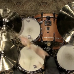
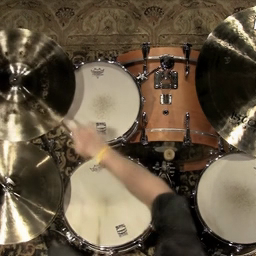
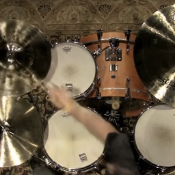
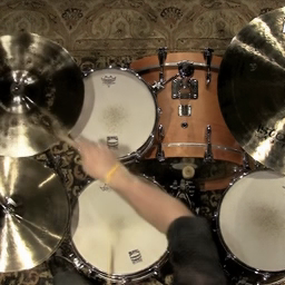
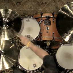
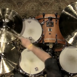
| Cello | Quintet | Drums | Talking Head | |||||||||||||
| SSIM () | LPIPS () | FVD () | SSIM () | LPIPS () | FVD () | SSIM () | LPIPS () | FVD () | SSIM () | LPIPS () | FVD () | |||||
| Baseline (MfS) | ||||||||||||||||
| Baseline + | R+D-RNN | |||||||||||||||
| SaC | ||||||||||||||||
| acIN | ||||||||||||||||
| All Abv. + | ConvGRU | |||||||||||||||
| DirConvGRU | ||||||||||||||||
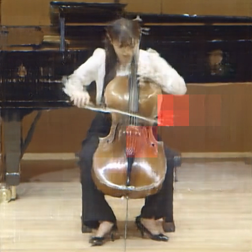
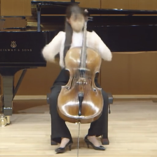
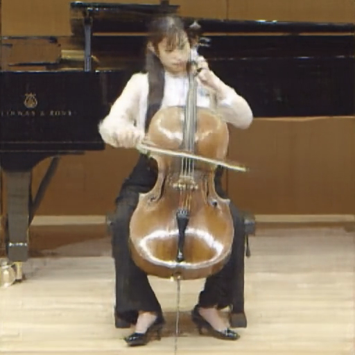
Skip vs. residual connections. In contrast to the observed in [33], the layer connection has a strong impact on the synthesis quality, where the main architectural difference with this work is the spatio-temporal cross-domain generation. As illustrated in Fig. 5, skip connections in the generator tend to produce large colored patches, increasing their presence and intensity as the input audio deviates from the original audio. Such glitches are probably induced by incorrect decisions taken in coarse low-level layers, and freely propagated through the outermost and finest layers. By switching to residual connections the artifacts simply disappear. Conversely, discriminators built upon residual connections often produce severe blurring and erase some details, see the face and bow in Fig. 5 (middle). Instead, a residual generator and skip-connected discriminators usually produce sharper images, see Fig. 5 (right). The fact that finer details can travel more cleanly to the low-level layers might help the image discriminator fit more precise data distribution and indirectly force the generator to synthesize more realistic images. The progressive growth generally lead to an unstable training, specially after each scale activation, and the multi-scale gradients variant was unable to conform coherent imaging.
Ablation study. A series of experiments were conducted on diverse audiovisual content of various minutes in length, as summarized in Footnote 5. Two perceptual objective image quality metrics, SSIM [69] and LPIPS [75], and one video quality metric FVD666From this implementation [56]. [61] were used. We observed a clear tendency to objectively improve not only image but also video quality by adding independently each proposed feature. Moreover, video prediction layers, and in particular DirConvGRU more than a basic ConvGRU, provided an extra boost of temporal enhancement.
Robustness to sound replacement. Synthesized images get affected when the distribution of feedforward sound deviates from the training source. This could be of interest to re-animate a video by using sounds from different contexts or acoustics. To evaluate this, random audio clips were selected from FSD50K [21]. Since large variations in distribution are plausibly expected, specially in terms of temporal dynamics, we cannot trust on FVD, while SSIM and LPIPS are simply infeasible in the absence of ground-truth pairs. Instead, FID [28] can measure distortions by comparing how far real and synthetic images are at high-level representation. From the results in Tab. 2, the full model proves more robustness on in-the-wild sound replacement when trained on a music video, while apparently the generalization capability reduces when trained on speech.
| FID () | Cello | Quintet | Drums | Talking Head |
|---|---|---|---|---|
| Baseline (MfS) | ||||
| Full Model |
Qualitative results. Our model is able to synthesize expressive long video sequences by synchronously responding to audio, without apparent degradation over time. Some illustrative examples are shown in Fig. 6. The combined sound routing significantly reduces artifacts, especially when the input sound deviates from the original audio distribution, in accordance with Footnote 5 and Tab. 2. Also, the video prediction layer tends to generate smoother motions and reduced flickering. Nevertheless, the persistence of temporal artifacts certainly affects the overall realism, specially for complex or sound-uncorrelated visual dynamics.


6 Discussion
In this work various strategies to improve temporal coherence of sound-to-video GANs have been proposed, which can be applied straightforwardly to other domains. Many other configurations were tested, including sound encoding [47, 64], conditioning augmentation [74], spectral and pixel normalization, joint audio-image discriminators, or feature matching loss [66, 6]. Most of them did not show improvements and, in general, any strategy to encode (compress) audio features led to an impairment.
Limitations. While our method struggles to reproduce large and complex motion dynamics, specially those unrelated to sound, it is particularly demanding on both computation and memory despite our amenable DirConvRNN.
Broader impact. Generative models like this can certainly leverage smart tools for audiovisual content creation. On the other hand, unlike images, there is still a significant gap to achieve high-quality realistic videos. Even so, it may already raise important ethical concerns on inappropriate usage, from faking reality to illicit activities.
Acknowledgements
This work was financially supported by the Catalan Government through the funding grant ACCIÓ-Eurecat (Project PRIV - DeepArts).
References
- [1] Dinesh Acharya, Zhiwu Huang, Danda Pani Paudel, and Luc Van Gool. Towards high resolution video generation with progressive growing of sliced wasserstein gans. ArXiv, abs/1810.02419, 2018.
- [2] Yogesh Balaji, Martin Renqiang Min, Bing Bai, Rama Chellappa, and Hans Peter Graf. Conditional gan with discriminative filter generation for text-to-video synthesis. In IJCAI, volume 1, page 2, 2019.
- [3] Nicolas Ballas, Li Yao, Chris Pal, and Aaron C. Courville. Delving deeper into convolutional networks for learning video representations. In 4th International Conference on Learning Representations, 2016.
- [4] Andrew Brock, Jeff Donahue, and Karen Simonyan. Large scale GAN training for high fidelity natural image synthesis. In 7th International Conference on Learning Representations, 2019.
- [5] Wonmin Byeon, Qin Wang, Rupesh Kumar Srivastava, and Petros Koumoutsakos. Contextvp: Fully context-aware video prediction. In ECCV, 2018.
- [6] Caroline Chan, Shiry Ginosar, Tinghui Zhou, and Alexei A. Efros. Everybody dance now. 2019 IEEE/CVF International Conference on Computer Vision (ICCV), pages 5932–5941, 2019.
- [7] Shiyu Chang, Yang Zhang, Wei Han, Mo Yu, Xiaoxiao Guo, Wei Tan, Xiaodong Cui, Michael Witbrock, Mark A Hasegawa-Johnson, and Thomas S Huang. Dilated recurrent neural networks. Advances in neural information processing systems, 30, 2017.
- [8] Moitreya Chatterjee and Anoop Cherian. Sound2sight: Generating visual dynamics from sound and context. In European Conference on Computer Vision, pages 701–719. Springer, 2020.
- [9] Kan Chen, Chuanxi Zhang, Chen Fang, Zhaowen Wang, Trung Bui, and Ram Nevatia. Visually indicated sound generation by perceptually optimized classification. In Proceedings of the European Conference on Computer Vision (ECCV) Workshops, pages 0–0, 2018.
- [10] Lele Chen, Zhiheng Li, Ross K Maddox, Zhiyao Duan, and Chenliang Xu. Lip movements generation at a glance. In Proceedings of the European Conference on Computer Vision (ECCV), pages 520–535, 2018.
- [11] Lele Chen, Ross K. Maddox, Zhiyao Duan, and Chenliang Xu. Hierarchical cross-modal talking face generation with dynamic pixel-wise loss. 2019 IEEE/CVF Conference on Computer Vision and Pattern Recognition (CVPR), pages 7824–7833, 2019.
- [12] Lele Chen, Sudhanshu Srivastava, Zhiyao Duan, and Chenliang Xu. Deep cross-modal audio-visual generation. In Proceedings of the on Thematic Workshops of ACM Multimedia 2017, pages 349–357, 2017.
- [13] Peihao Chen, Yang Zhang, Mingkui Tan, Hongdong Xiao, Deng Huang, and Chuang Gan. Generating visually aligned sound from videos. IEEE Transactions on Image Processing, 29:8292–8302, 2020.
- [14] Junyoung Chung, Caglar Gulcehre, Kyunghyun Cho, and Yoshua Bengio. Empirical evaluation of gated recurrent neural networks on sequence modeling. In NIPS 2014 Workshop on Deep Learning, December 2014, 2014.
- [15] Thomas H. Crystal and Arthur S. House. The duration of american-english vowels: an overview. Journal of Phonetics, 16:263–284, 1988.
- [16] Kangle Deng, Tianyi Fei, Xin Huang, and Yuxin Peng. Irc-gan: Introspective recurrent convolutional gan for text-to-video generation. In IJCAI, pages 2216–2222, 2019.
- [17] Chris Donahue, Julian McAuley, and Miller Puckette. Adversarial audio synthesis. In ICLR, 2019.
- [18] Bin Duan, Wei Wang, Hao Tang, Hugo Latapie, and Yan Yan. Cascade attention guided residue learning gan for cross-modal translation. In 2020 25th International Conference on Pattern Recognition (ICPR), pages 1336–1343. IEEE, 2021.
- [19] Jesse Engel, Kumar Krishna Agrawal, Shuo Chen, Ishaan Gulrajani, Chris Donahue, and Adam Roberts. GANSynth: Adversarial neural audio synthesis. In International Conference on Learning Representations, 2019.
- [20] Ruili Feng, Deli Zhao, and Zheng-Jun Zha. Understanding noise injection in gans. In International Conference on Machine Learning, pages 3284–3293. PMLR, 2021.
- [21] Eduardo Fonseca, Xavier Favory, Jordi Pons, Frederic Font, and Xavier Serra. FSD50K: an open dataset of human-labeled sound events. IEEE/ACM Transactions on Audio, Speech, and Language Processing, 30:829–852, 2022.
- [22] Songwei Ge, Thomas Hayes, Harry Yang, Xi Yin, Guan Pang, David Jacobs, Jia-Bin Huang, and Devi Parikh. Long video generation with time-agnostic vqgan and time-sensitive transformer. arXiv preprint arXiv:2204.03638, 2022.
- [23] Ian Goodfellow, Jean Pouget-Abadie, Mehdi Mirza, Bing Xu, David Warde-Farley, Sherjil Ozair, Aaron Courville, and Yoshua Bengio. Generative adversarial nets. Advances in neural information processing systems, 27, 2014.
- [24] Ishaan Gulrajani, Faruk Ahmed, Martin Arjovsky, Vincent Dumoulin, and Aaron C Courville. Improved training of wasserstein gans. Advances in neural information processing systems, 30, 2017.
- [25] Yudong Guo, Keyu Chen, Sen Liang, Yong-Jin Liu, Hujun Bao, and Juyong Zhang. Ad-nerf: Audio driven neural radiance fields for talking head synthesis. In Proceedings of the IEEE/CVF International Conference on Computer Vision, pages 5784–5794, 2021.
- [26] Ligong Han, Jian Ren, Hsin-Ying Lee, Francesco Barbieri, Kyle Olszewski, Shervin Minaee, Dimitris Metaxas, and Sergey Tulyakov. Show me what and tell me how: Video synthesis via multimodal conditioning. In Proceedings of the IEEE/CVF Conference on Computer Vision and Pattern Recognition, pages 3615–3625, 2022.
- [27] Wangli Hao, Zhaoxiang Zhang, and He Guan. Cmcgan: A uniform framework for cross-modal visual-audio mutual generation. In Proceedings of the AAAI conference on artificial intelligence, volume 32, 2018.
- [28] Martin Heusel, Hubert Ramsauer, Thomas Unterthiner, Bernhard Nessler, and Sepp Hochreiter. Gans trained by a two time-scale update rule converge to a local nash equilibrium. In NIPS, 2017.
- [29] Phillip Isola, Jun-Yan Zhu, Tinghui Zhou, and Alexei A Efros. Image-to-image translation with conditional adversarial networks. In Proceedings of the IEEE conference on computer vision and pattern recognition, pages 1125–1134, 2017.
- [30] Justin Johnson, Alexandre Alahi, and Li Fei-Fei. Perceptual losses for real-time style transfer and super-resolution. In European conference on computer vision, pages 694–711. Springer, 2016.
- [31] Emmanuel Kahembwe and Subramanian Ramamoorthy. Lower dimensional kernels for video discriminators. Neural networks : the official journal of the International Neural Network Society, 132:506–520, 2020.
- [32] Tero Karras, Samuli Laine, and Timo Aila. A style-based generator architecture for generative adversarial networks. In Proceedings of the IEEE/CVF conference on computer vision and pattern recognition, pages 4401–4410, 2019.
- [33] Tero Karras, Samuli Laine, Miika Aittala, Janne Hellsten, Jaakko Lehtinen, and Timo Aila. Analyzing and improving the image quality of stylegan. In Proceedings of the IEEE/CVF conference on computer vision and pattern recognition, pages 8110–8119, 2020.
- [34] Doyeon Kim, Donggyu Joo, and Junmo Kim. Tivgan: Text to image to video generation with step-by-step evolutionary generator. IEEE Access, 8:153113–153122, 2020.
- [35] Diederik P. Kingma and Jimmy Ba. Adam: A method for stochastic optimization. In 3rd International Conference on Learning Representations, 2015.
- [36] Kundan Kumar, Rithesh Kumar, Thibault de Boissière, Lucas Gestin, Wei Zhen Teoh, Jose M. R. Sotelo, Alexandre de Brébisson, Yoshua Bengio, and Aaron C. Courville. Melgan: Generative adversarial networks for conditional waveform synthesis. In NeurIPS, 2019.
- [37] Karol Kurach, Mario Lučić, Xiaohua Zhai, Marcin Michalski, and Sylvain Gelly. A large-scale study on regularization and normalization in gans. In International conference on machine learning, pages 3581–3590. PMLR, 2019.
- [38] Guillaume Le Moing, Jean Ponce, and Cordelia Schmid. Ccvs: context-aware controllable video synthesis. Advances in Neural Information Processing Systems, 34:14042–14055, 2021.
- [39] Seung Hyun Lee, Gyeongrok Oh, Wonmin Byeon, Jihyun Bae, ChanYoung Kim, Wonjae Ryoo, Sang Ho Yoon, Jinkyu Kim, and Sangpil Kim. Sound-guided semantic video generation. In ECCV, 2022.
- [40] Jiguo Li, Xinfeng Zhang, Chuanmin Jia, Jizheng Xu, Li Zhang, Y. Wang, Siwei Ma, and Wen Gao. Direct speech-to-image translation. IEEE Journal of Selected Topics in Signal Processing, 14:517–529, 2020.
- [41] Yitong Li, Martin Renqiang Min, Dinghan Shen, David Edwin Carlson, and Lawrence Carin. Video generation from text. In AAAI, 2018.
- [42] Jiadong Liang, Wenjie Pei, and Feng Lu. Cpgan: Content-parsing generative adversarial networks for text-to-image synthesis. In ECCV, 2020.
- [43] Xiaodan Liang, Lisa Lee, Wei Dai, and Eric P. Xing. Dual motion gan for future-flow embedded video prediction. 2017 IEEE International Conference on Computer Vision (ICCV), pages 1762–1770, 2017.
- [44] Mario Lucic, Karol Kurach, Marcin Michalski, Sylvain Gelly, and Olivier Bousquet. Are gans created equal? a large-scale study. In NeurIPS, 2018.
- [45] Mishaim Malik, Muhammad Kamran Malik, Khawar Mehmood, and Imran Makhdoom. Automatic speech recognition: a survey. Multim. Tools Appl., 80:9411–9457, 2021.
- [46] Javier Nistal, Stefan Lattner, and Gaël Richard. Drumgan: Synthesis of drum sounds with timbral feature conditioning using generative adversarial networks. In ISMIR, 2020.
- [47] Andrew Owens and Alexei A. Efros. Audio-visual scene analysis with self-supervised multisensory features. In ECCV, 2018.
- [48] Yingwei Pan, Zhaofan Qiu, Ting Yao, Houqiang Li, and Tao Mei. To create what you tell: Generating videos from captions. In Proceedings of the 25th ACM international conference on Multimedia, pages 1789–1798, 2017.
- [49] Hai Xuan Pham, Samuel Cheung, and Vladimir Pavlovic. Speech-driven 3d facial animation with implicit emotional awareness: A deep learning approach. 2017 IEEE Conference on Computer Vision and Pattern Recognition Workshops (CVPRW), pages 2328–2336, 2017.
- [50] Albert Pumarola, Antonio Agudo, Aleix M Martinez, Alberto Sanfeliu, and Francesc Moreno-Noguer. Ganimation: Anatomically-aware facial animation from a single image. In Proceedings of the European conference on computer vision (ECCV), pages 818–833, 2018.
- [51] Alec Radford, Luke Metz, and Soumith Chintala. Unsupervised representation learning with deep convolutional generative adversarial networks. arXiv preprint arXiv:1511.06434, 2015.
- [52] Scott Reed, Zeynep Akata, Xinchen Yan, Lajanugen Logeswaran, Bernt Schiele, and Honglak Lee. Generative adversarial text to image synthesis. In International conference on machine learning, pages 1060–1069. PMLR, 2016.
- [53] Masaki Saito, Eiichi Matsumoto, and Shunta Saito. Temporal generative adversarial nets with singular value clipping. In Proceedings of the IEEE international conference on computer vision, pages 2830–2839, 2017.
- [54] Masaki Saito, Shunta Saito, Masanori Koyama, and Sosuke Kobayashi. Train sparsely, generate densely: Memory-efficient unsupervised training of high-resolution temporal gan. International Journal of Computer Vision, 128(10):2586–2606, 2020.
- [55] Xingjian Shi, Zhourong Chen, Hao Wang, Dit-Yan Yeung, Wai-Kin Wong, and Wang-chun Woo. Convolutional lstm network: A machine learning approach for precipitation nowcasting. Advances in neural information processing systems, 28, 2015.
- [56] Ivan Skorokhodov, Sergey Tulyakov, and Mohamed Elhoseiny. Stylegan-v: A continuous video generator with the price, image quality and perks of stylegan2. In Proceedings of the IEEE/CVF Conference on Computer Vision and Pattern Recognition, pages 3626–3636, 2022.
- [57] Yang Song, Jingwen Zhu, Dawei Li, Andy Wang, and Hairong Qi. Talking face generation by conditional recurrent adversarial network. In Proceedings of the 28th International Joint Conference on Artificial Intelligence, pages 919–925. AAAI Press, 2019.
- [58] Marijn F Stollenga, Wonmin Byeon, Marcus Liwicki, and Juergen Schmidhuber. Parallel multi-dimensional lstm, with application to fast biomedical volumetric image segmentation. Advances in neural information processing systems, 28, 2015.
- [59] Yu Tian, Jian Ren, Menglei Chai, Kyle Olszewski, Xi Peng, Dimitris N. Metaxas, and Sergey Tulyakov. A good image generator is what you need for high-resolution video synthesis. In International Conference on Learning Representations, 2021.
- [60] Sergey Tulyakov, Ming-Yu Liu, Xiaodong Yang, and Jan Kautz. Mocogan: Decomposing motion and content for video generation. In Proceedings of the IEEE conference on computer vision and pattern recognition, pages 1526–1535, 2018.
- [61] Thomas Unterthiner, Sjoerd van Steenkiste, Karol Kurach, Raphaël Marinier, Marcin Michalski, and Sylvain Gelly. Towards accurate generative models of video: A new metric & challenges. ArXiv, abs/1812.01717, 2018.
- [62] Aäron van den Oord, Sander Dieleman, Heiga Zen, Karen Simonyan, Oriol Vinyals, Alex Graves, Nal Kalchbrenner, Andrew W. Senior, and Koray Kavukcuoglu. Wavenet: A generative model for raw audio. In Proc. 9th ISCA Workshop on Speech Synthesis Workshop (SSW 9), page 125, 2016.
- [63] Konstantinos Vougioukas, Stavros Petridis, and Maja Pantic. Realistic speech-driven facial animation with gans. International Journal of Computer Vision, 128:1398–1413, 2019.
- [64] Chia-Hung Wan, Shun-Po Chuang, and Hung yi Lee. Towards audio to scene image synthesis using generative adversarial network. ICASSP 2019 - 2019 IEEE International Conference on Acoustics, Speech and Signal Processing (ICASSP), pages 496–500, 2019.
- [65] Kaisiyuan Wang, Qianyi Wu, Linsen Song, Zhuoqian Yang, Wayne Wu, Chen Qian, Ran He, Yu Qiao, and Chen Change Loy. Mead: A large-scale audio-visual dataset for emotional talking-face generation. In Computer Vision–ECCV 2020: 16th European Conference, Glasgow, UK, August 23–28, 2020, Proceedings, Part XXI, pages 700–717. Springer, 2020.
- [66] Ting-Chun Wang, Ming-Yu Liu, Jun-Yan Zhu, Guilin Liu, Andrew Tao, Jan Kautz, and Bryan Catanzaro. Video-to-video synthesis. arXiv preprint arXiv:1808.06601, 2018.
- [67] Ting-Chun Wang, Ming-Yu Liu, Jun-Yan Zhu, Andrew Tao, Jan Kautz, and Bryan Catanzaro. High-resolution image synthesis and semantic manipulation with conditional gans. 2018 IEEE/CVF Conference on Computer Vision and Pattern Recognition, pages 8798–8807, 2018.
- [68] Yaohui Wang, Piotr Bilinski, Francois Bremond, and Antitza Dantcheva. G3an: Disentangling appearance and motion for video generation. In Proceedings of the IEEE/CVF Conference on Computer Vision and Pattern Recognition, pages 5264–5273, 2020.
- [69] Zhou Wang, Alan Conrad Bovik, Hamid R. Sheikh, and Eero P. Simoncelli. Image quality assessment: from error visibility to structural similarity. IEEE Transactions on Image Processing, 13:600–612, 2004.
- [70] Tao Xu, Pengchuan Zhang, Qiuyuan Huang, Han Zhang, Zhe Gan, Xiaolei Huang, and Xiaodong He. Attngan: Fine-grained text to image generation with attentional generative adversarial networks. In Proceedings of the IEEE conference on computer vision and pattern recognition, pages 1316–1324, 2018.
- [71] Pei-Tse Yang, Feng-Guang Su, and Yu-Chiang Frank Wang. Diverse audio-to-image generation via semantics and feature consistency. In 2020 Asia-Pacific Signal and Information Processing Association Annual Summit and Conference (APSIPA ASC), pages 1188–1192. IEEE, 2020.
- [72] V. Yushchenko, Nikita Araslanov, and Stefan Roth. Markov decision process for video generation. 2019 IEEE/CVF International Conference on Computer Vision Workshop (ICCVW), pages 1523–1532, 2019.
- [73] Han Zhang, Jing Yu Koh, Jason Baldridge, Honglak Lee, and Yinfei Yang. Cross-modal contrastive learning for text-to-image generation. 2021 IEEE/CVF Conference on Computer Vision and Pattern Recognition (CVPR), pages 833–842, 2021.
- [74] Han Zhang, Tao Xu, Hongsheng Li, Shaoting Zhang, Xiaogang Wang, Xiaolei Huang, and Dimitris N Metaxas. Stackgan: Text to photo-realistic image synthesis with stacked generative adversarial networks. In Proceedings of the IEEE international conference on computer vision, pages 5907–5915, 2017.
- [75] Richard Zhang, Phillip Isola, Alexei A. Efros, Eli Shechtman, and Oliver Wang. The unreasonable effectiveness of deep features as a perceptual metric. 2018 IEEE/CVF Conference on Computer Vision and Pattern Recognition, pages 586–595, 2018.
- [76] Yi Zhao, Yanyan Shen, and Junjie Yao. Recurrent neural network for text classification with hierarchical multiscale dense connections. In IJCAI, 2019.
- [77] Hang Zhou, Yu Liu, Ziwei Liu, Ping Luo, and Xiaogang Wang. Talking face generation by adversarially disentangled audio-visual representation. In Proceedings of the AAAI conference on artificial intelligence, volume 33, pages 9299–9306, 2019.
- [78] Yipin Zhou, Zhaowen Wang, Chen Fang, Trung Bui, and Tamara L Berg. Visual to sound: Generating natural sound for videos in the wild. In Proceedings of the IEEE conference on computer vision and pattern recognition, pages 3550–3558, 2018.
- [79] Hao Zhu, Yi Li, Feixia Zhu, Aihua Zheng, and Ran He. Let’s play music: Audio-driven performance video generation. In 2020 25th International Conference on Pattern Recognition (ICPR), pages 3574–3581. IEEE, 2021.
- [80] Minfeng Zhu, Pingbo Pan, Wei Chen, and Yi Yang. Dm-gan: Dynamic memory generative adversarial networks for text-to-image synthesis. 2019 IEEE/CVF Conference on Computer Vision and Pattern Recognition (CVPR), pages 5795–5803, 2019.