Flux-Rope Mediated Turbulent Magnetic Reconnection

Abstract

We present a new model of magnetic reconnection in the presence of turbulence, applicable when the magnetic helicity is non-zero. The new model differs from the Lazarian-Vishniac turbulent reconnection theory by emphasizing the role of locally coherent magnetic structures, whose existence is shown to be permitted by the properties of magnetic field line separation in turbulent plasma. Local coherence allows storage of magnetic helicity inside the reconnection layer and we argue that helicity conservation produces locally coherent twisted flux ropes. We then introduce the “Alfvén horizon” to explain why the global reconnection rate can be governed by locally coherent magnetic field structure instead of by field line wandering, formally extending to 3D the principle that reconnection can be made fast by fragmentation of the global current layer. Coherence is shown to dominate over field line dispersion if the anisotropy of the turbulence at the perpendicular scale matching the thickness of a marginally stable current layer exceeds the aspect ratio of the current layer. Finally, we conjecture that turbulence generated within the reconnection layer may produce a balance of anisotropies that maintains the system in the flux-rope mediated regime. The new model successfully accounts for the major features of 3D numerical simulations of self-generated turbulent reconnection, including reconnection rates of 0.01 in resistive MHD and 0.1 with collisionless physics.

1 Introduction

Magnetic reconnection is a fundamental plasma process that enables the rapid reconfiguration of magnetic fields. It is strongly associated with plasma heating, jets and particle acceleration, and it is central to a wide range of explosive astrophysical phenomena including solar flares, coronal heating and auroral substorms. Magnetic reconnection also occurs in the laboratory, for example, during sawtooth crashes and flux rope merging. Introductions to the field can be found in the books by Priest & Forbes (2000), Birn & Priest (2007) and Yamada (2022).

The first quantitative model of magnetic reconnection (Sweet, 1958; Parker, 1957) examined a laminar steady-state current sheet in resistive MHD, finding that the reconnection rate (specified as the Alfvén Mach number of the inflow) satisfies

$$\frac{V_{rec}^{SP}}{V_{A}}=S_{L}^{-1/2}.$$ (1)

The right-hand side depends on the Lundquist number,

$$S_{L}=\frac{LV_{A}}{\eta},$$ (2)

where $L$ is the half length of the reconnection layer, $V_{A}$ is the Alfvén speed and $\eta=1/\mu_{0}\sigma$ is the magnetic diffusivity. It is well known that evaluating Eq (1) for a typical coronal Lundquist number (say $10^{12}$) yields a reconnection rate ($10^{-6}$) that is vastly smaller than empirical rates of 0.01–0.1 inferred from solar flare observations.

The rate problem with Sweet-Parker reconnection was recognized immediately and various solutions have been explored. The most notable are Petschek reconnection (Petschek, 1964), reconnection with collisionless effects such as the Hall electric field (Birn et al., 2001), turbulent reconnection (Lazarian & Vishniac, 1999; Kowal et al., 2009), and plasmoid mediated reconnection (Lapenta, 2008; Cassak et al., 2009; Bhattacharjee et al., 2009; Huang & Bhattacharjee, 2010; Uzdensky et al., 2010). All of the aforementioned models produce acceptably fast reconnection rates.

Recently, the scientific community has increasingly focused on the cross-scale coupling required to connect the global length scales with the much smaller scales on which field lines reconnect. In this context, the central role of plasmoids in 2D reconnection is well understood (Huang & Bhattacharjee, 2010; Uzdensky et al., 2010) but it has not yet been conclusively established if the same mechanism carries over to 3D, or if instead the reconnection rate is determined by fully 3D phenomena such as field line dispersion due to turbulence (Lazarian & Vishniac, 1999; Kowal et al., 2009). We also allow that different mechanisms may dominate under different conditions. Attempts to resolve these problems have been described as the “third phase of magnetic reconnection research” (Ji et al., 2023).

In the study of solar flares, there is a long-standing association between turbulence and magnetic reconnection. Specifically, the well documented nonthermal broadening of hot spectral lines is widely considered to be direct evidence of turbulent motions. A review covering historical and modern observations and their interpretation has been given by Russell (2024). Russell (2024) also explores the generation mechanisms of turbulence in solar flares and its connection to reconnection.

Focusing here on recent observational results, space instruments have found motions of hundreds of km s^-1 in the above-the-loop region of solar flares (Doschek et al., 2014; Kontar et al., 2017; Stores et al., 2021; Shen et al., 2023) and in post-CME plasma sheets (Ciaravella et al., 2002; Ciaravella & Raymond, 2008; Bemporad, 2008; Susino et al., 2013; Warren et al., 2018; Li et al., 2018; Cheng et al., 2018; French et al., 2020). The closeness of the relationship between turbulence and reconnection in solar flares is demonstrated by the detection of turbulence tens of seconds before impulsive phenomena: the papers by Jeffrey et al. (2018) and Chitta & Lazarian (2020) provide modern examples; also see earlier evidence on timings by Antonucci et al. (1984), Alexander et al. (1998), Harra et al. (2001) and Ranns et al. (2001). Insight into why turbulence and fast reconnection develop side-by-side has recently come from work by French et al. (2021) and Wyper & Pontin (2021), who studied the substructure of flare ribbons around the onset of the impulsive phase. Both studies concluded that fast reconnection begins after a coronal current sheet becomes unstable to tearing instability which develops nonlinearly into turbulence, with French et al. (2021) showing that ribbon substructure grows fastest at a key scale then spreads to larger and smaller scales.

The scenario of tearing instability developing into turbulence as reconnection becomes fast is also supported by direct numerical simulations. While the first numerical investigations of turbulent reconnection were driven by a forcing term added to the momentum equation (Kowal et al., 2009), the frontier of high performance computing has recently crossed a threshold beyond which turbulence develops by itself within 3D magnetic reconnection simulations. Turbulence is self-generated when the scale separation exceeds a critical threshold (canonically $S_{c}=10^{4}$ in resistive MHD) above which an initial Sweet-Parker current layer is unstable to a fast tearing instability (Furth et al., 1963; Bulanov et al., 1978; Biskamp, 1986; Loureiro et al., 2007; Baalrud et al., 2012). When $S_{L}\gg S_{c}$, the tearing instability can operate recursively, as proposed by Shibata & Tanuma (2001). In 3D, the ensuing nonlinear evolution generates and sustains turbulence within the reconnection layer. Self-generated turbulent reconnection (SGTR) simulations of this type have now been reported by many investigators, using both collisionless codes (Daughton et al., 2011, 2014; Liu et al., 2013; Pritchett, 2013; Nakamura et al., 2013, 2017; Dahlin et al., 2015, 2017; Le et al., 2018; Stanier et al., 2019; Li et al., 2019; Agudelo Rueda et al., 2021; Zhang et al., 2021) and resistive MHD codes (Oishi et al., 2015; Huang & Bhattacharjee, 2016; Striani et al., 2016; Beresnyak, 2017; Kowal et al., 2017, 2020; Yang et al., 2020; Beg et al., 2022).

A current dichotomy is that SGTR simulations exhibit many features anticipated by the Lazarian & Vishniac (1999) theory of turbulent reconnection, including fast reconnection rates, power law spectra and dispersion of magnetic field lines. However, they also exhibit features that are strongly reminiscent of 2D plasmoid mediated reconnection, such as the presence of flux ropes in the reconnection layer and an excellent match of the reconnection rate (Daughton et al., 2014; Huang & Bhattacharjee, 2016; Beg et al., 2022). The present paper aims to develop the theory of 3D magnetic reconnection with self-generated turbulence by addressing the roles of coherent magnetic strutures and magnetic helicity. We propose a new conceptual model that reconciles aspects of the 3D Lazarian-Vishniac turbulent reconnection theory and 2D plasmoid mediated reconnection. The new model successfully accounts for the main features seen in SGTR simulations that reach a statistically stationary state, including the reconnection rate.

The article is structured as follows. Section 2 investigates the dispersion of magnetic field lines in turbulent plasma, showing that while field line wandering dominates over long trace distances, magnetic field structures are coherent for shorter trace distances. The nature of the coherent structures is investigated in Section 3, where we propose that conservation of magnetic helicity produces locally coherent flux ropes inside the reconnection layer and consider their interactions. In Section 4, we introduce the concept of the Alfvén horizon and using this to show that coherent structures can govern the global reconnection rate as opposed to the field line dispersion. The paper concludes with a discussion in Section 5 and summary in Section 6. The articles by Lazarian & Vishniac (1999) and Beg et al. (2022) are referred to frequently, so we abbreviate them as LV99 and BRH22.

2 Magnetic Field Line Separation in Turbulent Plasma

We begin by investigating the dispersion of magnetic field lines in turbulent plasma, exploring how the mean square separation between field line pairs $\left<\delta^{2}\right>$ depends on the trace distance $s$ and the initial separation $\delta_{0}$. The value of $\left<\delta^{2}\right>$ tracks the cross-sectional area over which field lines have been dispersed, while the root mean square (rms) separation $\left<\delta^{2}\right>^{1/2}$ measures the average distance between field line pairs. Our modeling approach follows LV99 with the important difference that we treat the initial separation distance between field line pairs without setting it to zero.

2.1 Derivation

We consider the average behavior over many field line pairs, making a continuum approach suitable, and adopt Eq (4) of LV99,

$$\frac{d\left<\delta^{2}\right>}{ds}=k_{\parallel}\left<\delta^{2}\right>,$$ (3)

where $k_{\parallel}^{-1}$ is the characteristic length scale governing scattering of magnetic field lines. If $k_{\parallel}$ is independent of $\left<\delta^{2}\right>$ then Eq (3) yields the exponentiation relation $\left<\delta^{2}\right>=\delta_{0}^{2}\exp(k_{\parallel}s)$.

When field lines are scattered by turbulence, one must take into account that $k_{\parallel}$ for a magnetic eddy depends on $k_{\perp}$. In this paper, we consider scaling relations of the form

$$k_{\parallel}=Ck_{\perp}^{a},$$ (4)

where the proportionality factor $C$ and the index $a$ are properties of the turbulence. Equation (4) is equivalent to a scale-dependent anisotropy relation

$$\frac{k_{\parallel}}{k_{\perp}}=Ck_{\perp}^{a-1}.$$ (5)

For MHD turbulence, one typically has $0<a\leq 1$. If $0<a<1$ then the magnetic eddies become increasingly elongated along the background magnetic field with decreasing perpendicular scale, consistent with the filamentation that is characteristic of magnetized plasmas. The Goldreich & Sridhar (1995) turbulence adopted by LV99 satisfies Eq (4) with $a=2/3$ and $C=l_{inj}^{a-1}(v_{inj}/V_{A})^{4/3}$, where $v_{inj}$ is the velocity amplitude at injection scale $l_{inj}$. Direct numerical simulations of self-generated reconnection turbulence by Kowal et al. (2017) support the $a=2/3$ scaling. In the special case of $a=1$, the anisotropy is scale-independent, as was reported for the SGTR simulation by Huang & Bhattacharjee (2016).

Using Eq (4) to substitute for $k_{\parallel}$ in Eq (3), and making the identification $k_{\perp}=\left<\delta^{2}\right>^{-1/2}$, we obtain

$$\frac{d\left<\delta^{2}\right>}{ds}=C\left<\delta^{2}\right>^{1-a/2},$$ (6)

which is a separable ordinary differential equation for $\left<\delta^{2}\right>$. Provided that $a\neq 0$ (avoiding the exponentiation case dealt with separately above) the solution is

$$\left<\delta^{2}\right>=\left(\delta_{0}^{a}+\gamma s\right)^{2/a},$$ (7)

where $\gamma=Ca/2$. When analyzing a numerical simulation or an experiment, it may often be easier to obtain $\gamma$ by fitting Eq (7) than to infer it indirectly from $a$ and $C$. The $\delta_{0}$ that appears in Eq (7) comes from the constant of integration, which was not included by LV99. Its inclusion is central to the present paper.

2.2 Richardson Dispersion

For infinitesimal $\delta_{0}\to 0$ or large $s\to\infty$, Eq (7) behaves asymptotically as

$$\left<\delta^{2}\right>\approx\left(\gamma s\right)^{2/a}.$$ (8)

In this limit, the average separation of field line pairs is fully determined by the trace distance $s$ and the turbulence properties $\gamma$ and $a$, whereas the original separation $\delta_{0}$ has been forgotten. The $\left<\delta^{2}\right>\sim s^{2/a}$ scaling in Eq (8) implies that turbulence with $a<2$ disperses magnetic field lines faster than Brownian diffusion, which has $\left<\delta^{2}\right>\sim s$. If $a<1$ such that small-scale magnetic eddies have greater $k_{\perp}/k_{\parallel}$ than large-scale eddies, then the rms separation $\left<\delta^{2}\right>^{1/2}$ increases superlinearly with respect to $s$.

In the specific case of the Goldreich & Sridhar (1995) scalings, Eq (8) yields

$$\left<\delta^{2}\right>\approx\left(\frac{v_{inj}}{V_{A}}\right)^{4}\frac{\left(3s\right)^{3}}{l_{inj}},$$ (9)

which recovers the Richardson dispersion scaling $\left<\delta^{2}\right>\sim s^{3}$ obtained by LV99.

LV99 noted the assumptions used to derive Eq (6) eventually fail for $s\to\infty$, since the strong turbulence scalings are eventually replaced by diffusion at a maximal rate. Under these conditions, the right hand side of Eq (3) is replaced with a constant, thus Richardson-type dispersion eventually gives way to Brownian diffusion with $\left<\delta^{2}\right>\sim s$. In a bounded domain, $<\delta^{2}>^{1/2}$ is also bounded by the domain size.

2.3 Local Coherence

The most important difference between Eq (7) and the corresponding derivation in LV99 is the inclusion of the initial separation distance. That is to say, we have retained the constant of integration introduced by integrating Eq (6), which was dropped by LV99. Examining the full solution given by Eq (7), the Richardson-type dispersion regime is only valid for $\gamma s\gg\delta_{0}^{a}$. Earlier in the field line tracing, $\gamma s\ll\delta_{0}^{a}$ gives $\left<\delta^{2}\right>^{1/2}\approx\delta_{0}$, which implies that the field line separation is determined by its initial value. This result allows the presence of locally coherent magnetic field structures, which we propose can have an important role in turbulent reconnection.

Figure 1 plots $\langle\delta^{2}\rangle^{1/2}$ based on Eq (7), setting $a=2/3$ consistent with Goldreich & Sridhar (1995), LV99 and Kowal et al. (2017). The thick black line shows the Richardson dispersion obtained by setting $\delta_{0}=0$, which is central to the LV99 theory of turbulent reconnection. The filled gray region is forbidden because Eq (7) implies $\langle\delta^{2}\rangle\geq(\gamma s)^{2/a}$, with equality only for $\delta_{0}=0$. Figure 1 also plots solutions for various non-zero initial separations: these curves are initially horizontal, corresponding to the result that turbulence initially has a negligible effect on the separation. Dispersion only takes over once the dotted horizontal line given by $\langle\delta^{2}\rangle^{1/2}\approx\delta_{0}$ nears the thick solid Richardson dispersion line given by Eq (8).

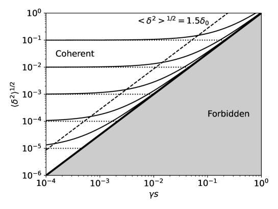
Figure 1: Root mean square (rms) field line separation $\langle\delta^{2}\rangle^{1/2}=(\delta_{0}^{a}+\gamma s)^{1/a}$, showing dependence on trace distance $s$ and initial separation $\delta_{0}$, plotted for the Goldreich & Sridhar (1995) anisotropy scaling index $a=2/3$. The thick black line shows the Richardson dispersion relation $\langle\delta^{2}\rangle^{1/2}=(\gamma s)^{1/a}$ obtained for $\delta_{0}=0$. The gray region is forbidden because rms field line separations cannot be smaller than the solution for $\delta_{0}=0$. Solution curves are shown for $\delta_{0}\in\left\{10^{-1},10^{-2},10^{-3},10^{-4},10^{-5}\right\}$ (thinner solid lines). Initially, $\langle\delta^{2}\rangle^{1/2}\approx\delta_{0}$, which allows the existence of locally coherent magnetic field structure in turbulent plasma. The scale-dependent transition between coherence and dispersion is highlighted by the dashed line, which curves cross when $\langle\delta^{2}\rangle^{1/2}=1.5\delta_{0}$.

Inspecting Eq (7), the transition between coherence and dispersion happens as $s$ approaches

$$s^{*}=\frac{\delta_{0}^{a}}{\gamma}.$$ (10)

It is evident that the trace distance over which magnetic structure remains coherent is scale-dependent, since the value of $s^{*}$ scales as $\delta_{0}^{a}$. Mathematically, Eq (10) matches the two terms inside the bracket on the right hand side of Eq (7). Physically, dispersion only affects a given length scale once a field line pair with infinitesimal initial separation has been dispersed to the scale of interest. This implies that structure any chosen scale mixes out after structure at all smaller scales, provided that $a>0$.

Equation (10) can be related to the parallel wavenumber of the turbulence at the perpendicular scale $\delta_{0}$. Using Eq (4), if $k_{\perp}$ is set to $\delta_{0}^{-1}$ then $k_{\parallel}(\delta_{0})=C\delta_{0}^{-a}$ and Eq (10) implies

$$s^{*}=\frac{2}{ak_{\parallel}(\delta_{0})}.$$ (11)

Thus, a pair of field lines must be traced a distance comparable to the parallel length scale of the turbulence (at the perpendicular scale of their initial separation) before field line dispersion by the turbulence becomes significant.

When $s=s^{*}$, the rms field line separation satisfies $\langle\delta^{2}\rangle^{1/2}=2^{1/a}\delta_{0}$. More generally, one might consider dispersion to be significant once $\langle\delta^{2}\rangle^{1/2}/\delta_{0}$ exceeds a value $f$ other than $2^{1/a}$. Using Eq (7), this general threshold is crossed at $s=s^{\dagger}$, where

$$s^{\dagger}=(f^{a}-1)s^{*}.$$ (12)

We consider a value of $f=1.5$ to be a useful indication that the field lines are beginning to separate. Curves in Figure 1 reach this threshold when they intersect the dashed line.

2.4 Section Summary

Magnetic fields in turbulent plasmas exhibit both dispersion and local coherence. Richardson-type dispersion occurs for longer trace distances and we note that this phenomenon is at the heart of the LV99 model of turbulent reconnection. However, by retaining a constant of integration, we have shown that the field line separation model solved by LV99 also exhibits local coherence, meaning that field line separations are unaffected by dispersion until they have been traced further than the parallel scale of the turbulence evaluated at the perpendicular scale matching the initial field line separation. We propose that the property of local coherence should also be taken into account in the theory of turbulent magnetic reconnection.

3 Magnetic Helicity and Flux Ropes

Having shown that turbulence permits the existence of locally coherent magnetic field structures, we now examine what form these structures should take inside a turbulent reconnection layer. The importance of magnetic helicity is highlighted and we propose that helicity conservation produces locally coherent flux ropes inside the reconnection layer, provided the reconnecting magnetic field has non-zero helicity.

3.1 Magnetic Helicity

Magnetic helicity quantifies the total linking of magnetic flux (Moffatt, 1969). In magnetically closed domains, the magnetic helicity is gauge-invariant and can calculated using the volume integral

$$H=\int_{V}\boldsymbol{A}\cdot\boldsymbol{B}\,d^{3}x,$$ (13)

where $\boldsymbol{A}$ a magnetic vector potential such that $\boldsymbol{B}=\nabla\times\boldsymbol{A}$ (Woltjer, 1958). Helicity can also be extended to magnetically open domains, either using the relative magnetic helicity, which is gauge-invariant but depends on a choice of reference magnetic field (Berger & Field, 1984; Finn & Antonsen, 1985), or by restricting the gauge of the vector potential to ensure that the helicity integral has a geometrical meaning (Prior & Yeates, 2014; Berger & Hornig, 2018; Prior & MacTaggart, 2020; Xiao et al., 2023). The relationship between magnetic helicity and current helicity has recently been discussed by Russell et al. (2019).

SGTR simulations are often initialized with a 2.5D magnetic field of the form $\boldsymbol{B}(x,y)$, where $z$ is the invariant direction. For 2.5D magnetic fields with $B_{z}\neq 0$, there is typically a net linking of magnetic flux so the magnetic helicity is non-zero. For example, the $\boldsymbol{B}$ that initialized the SGTR simulation by BRH22 has $H=-0.134$. This article considers turbulent reconnection in such “non-zero helicity” situations. In the special case of a purely 2D initial magnetic field with $B_{z}=0$, a vector potential of the form $\boldsymbol{A}=A(x,y)\boldsymbol{e}_{z}$ can be found giving $H=0$ from Eq (13). This “zero helicity” case corresponds to reconnection with a magnetic shear angle of 180 degrees. It is excluded from our present reconnection model but it will be discussed again in Section 5.4.

3.2 Helicity Conservation, Flux and Storage

In ideal MHD, the magnetic helicity is exactly conserved as a consequence of Alfvén’s theorem. It is also highly conserved during magnetic reconnection at high Lundquist numbers, which is the basis of Taylor relaxation (Taylor, 1974, 1986; Berger, 1984; Russell et al., 2015; Pontin et al., 2016; Yeates et al., 2021).

Here, we apply helicity conservation to the self-generated turbulent reconnection layer geometry sketched in Figure 2. We assume that the plasma is turbulent between the pair of stochastic separatrix surfaces that mark the upstream boundaries of the reconnection layer (these surfaces were computed for the SGTR simulations by BRH22 and Daughton et al. (2014)). Between the stochastic separatrix surfaces, turbulence disperses magnetic field lines for sufficiently long trace distances, whereas the magnetic fields upstream of the reconnection layer are treated as laminar, i.e. lying on flux surfaces. During reconnection, inflow of plasma carries fresh magnetic flux into the reconnection layer across the stochastic separatrix surfaces, and outflow jets expel reconnected magnetic flux.

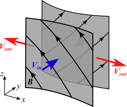
Figure 2: Sketch of the considered reconnection geometry. The gray surfaces represent the boundaries of the region inside which magnetic field lines are turbulently dispersed as examined in Section 2. The upstream magnetic field is treated as laminar with field lines lying on flux surfaces. The blue arrows indicate inflows of plasma into the reconnection layer, and the red arrows represent the outflows. Magnetic field lines are shown immediately upstream of the reconnection layer. Magnetic flux tubes entering the reconnection layer from opposite sides cross at an oblique angle, giving them non-zero mutual magnetic helicity.

To explore the helicity dynamics in a simple way, suppose that the regions upstream and downstream of the reconnection layer satisfy the ideal Ohm’s law, $\boldsymbol{E}=-\boldsymbol{V}\times\boldsymbol{B}$. One can then use the Ohm’s law and Maxwell’s equations to obtain the conservation equation

$$\frac{\partial}{\partial t}\left(\boldsymbol{A}\cdot\boldsymbol{B}\right)+\nabla\cdot\left[\left(\boldsymbol{A}\cdot\boldsymbol{B}\right)\boldsymbol{V}+\left(\Phi-\boldsymbol{A}\cdot\boldsymbol{V}\right)\boldsymbol{B}\right]=0,$$ (14)

where $\Phi$ is the scalar potential. The first contribution to the helicity flux, $\left(\boldsymbol{A}\cdot\boldsymbol{B}\right)\boldsymbol{V}$, represents transport with the fluid velocity. The other contribution to the helicity flux can be made to vanish by gauge transformation.

The $\left(\boldsymbol{A}\cdot\boldsymbol{B}\right)\boldsymbol{V}$ term implies that helicity density is transported into and out of the reconnection layer by the inflows and outflows, consistent with Alfvén’s theorem. On average, the helicity fluxes into and out of the reconnection layer balance, assuming negligible creation/destruction of magnetic helicity inside the reconnection layer (Taylor, 1974; Berger, 1984). Furthermore, since there is a time delay between when plasma enters the reconnection layer and when it exits the reconnection layer, magnetic helicity must be stored inside the reconnection layer at any given moment. We propose that the local coherence identified in Section 2 stores the magnetic helicity inside the reconnection layer.

3.3 Formation of Twisted Flux Ropes

We now turn to the question, “What type of locally coherent magnetic field structure stores the helicity inside the reconnection layer?” In answer we propose that the conservation of helicity creates twisted flux ropes. To a large extent this answer is known in advance since: (i) flux ropes have been extensively linked to reconnection at the Earth’s dayside magnetopause (Russell & Elphic, 1979; Lee & Fu, 1985), in Earth’s magnetotail (Zong et al., 2004; Chen et al., 2008) and in solar flares (Takasao et al., 2012, 2016; Cheng et al., 2018); (ii) flux ropes feature in 2D and 3D tearing instabilities (Furth et al., 1963; Loureiro et al., 2007; Baalrud et al., 2012); and (iii) their presence has been widely noted in SGTR simulations including Daughton et al. (2011), Huang & Bhattacharjee (2016) and BRH22.

Our novel contribution is the argument that flux ropes are a robust feature of magnetic reconnection with self-generated turbulence because: (a) local coherence is built into magnetic field line separations as shown in Section 2; and (b) the production of flux ropes is driven by helicity conservation. Therefore the flux ropes cannot be eliminated by increasing the Lundquist number or making the system more turbulent. The only way to remove them while conserving magnetic helicity is to reduce the absolute value of the helicity towards zero, as in the important case where the magnetic shear angle approaches 180 degrees. As already stated, we exclude that special case from the present paper which examines magnetic reconnection with non-zero magnetic helicity.

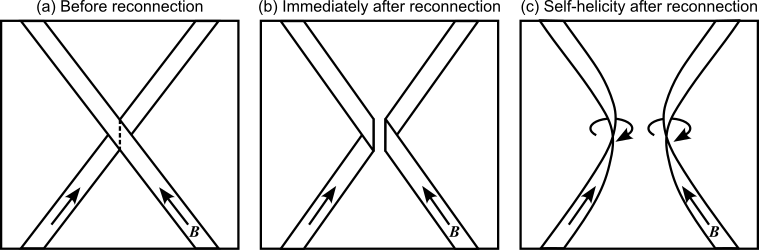
Figure 3: Conversion of mutual helicity to self helicity during reconnection of a pair of flux ribbons, based on an original cartoon by Wright & Berger (1989). The left panel (a) shows the original pair of flux ribbons. These cross which gives them mutual helicity. In this cartoon, magnetic reconnection is treated heuristically by cutting the ribbons along the dashed line in (a) and rejoining them as shown in the middle panel (b). The newly created flux ribbons no longer cross so the mutual helicity has been lost and this is compensated by the new flux ribbons having self helicity. The right panel (c) shows the new ribbons a short time after the reconnection. For this configuration, both new ribbons have a left handed twist.

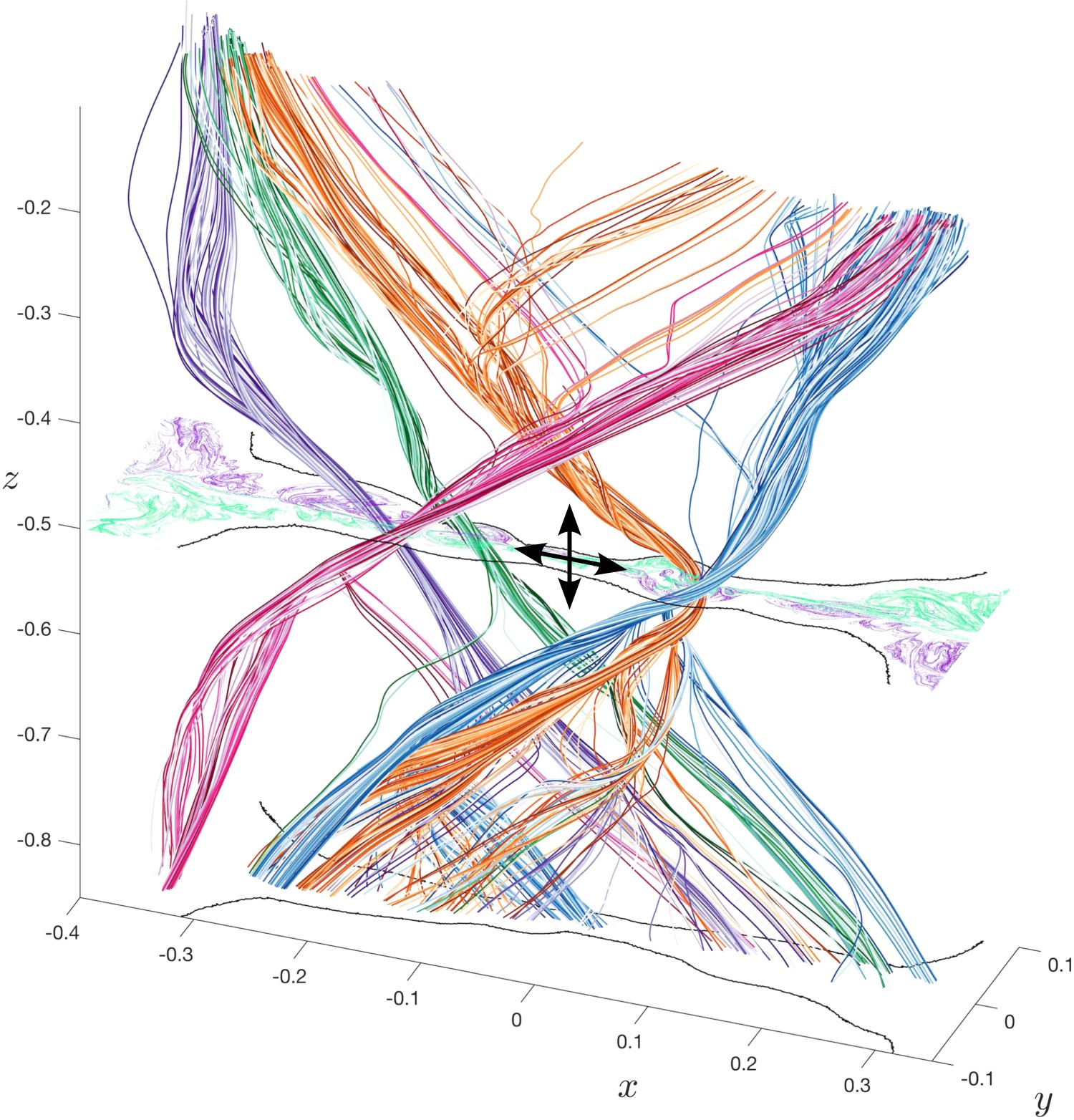
Figure 4: Magnetic field lines in an MHD simulation of self-generated turbulent reconnection by Beg et al. (2022). The black curves on $z=-0.5$ and $z=-1.0$ show where these planes intersect the stochastic spearatrices, which are the upstream boundaries of the turbulent reconnection layer. Magnetic field lines (multicolored) are traced inside the reconnection layer from seed points placed on the $z=-0.5$ plane. Over short trace distances, the field lines form locally coherent oblique twisted flux ropes. Over longer trace distances, dispersion dominates such that field lines from different flux ropes are highly intermixed by the time they reach the $z$ boundaries. Topological structure on the $z=-0.5$ cut is shown using maximizing ridges of the forward (green) and backward (purple) finite time Lyapunov exponent. The horizontal black arrows indicate a representative length of a microscopic current sheet between flux ropes. The vertical black arrows indicate the corresponding Alfvén horizon: the magnetic flux ropes are highly coherent over this distance. Adapted from Beg et al. (2022) under a CC-BY 4.0 license.

The total magnetic helicity can be decomposed as the sum of self and mutual helicities (Berger & Field, 1984). Typically, when a pair of flux tubes reconnects their mutual helicity changes and the self helicity must therefore change by an equal and opposite amount. This process produces twisted flux ropes, as can be illuminated using the following heuristic arguments adapted from Wright & Berger (1989) (also see Lee & Fu, 1985; Wright, 2019). Figure 3(a) shows a pair of flux ribbons on opposite sides of the reconnection layer. They cross each other and therefore have non-zero mutual helicity. In this scientific cartoon, reconnection cuts and rejoins the ribbons to make the new ones in panel (b). The new ribbons do not cross, so there has been a loss of mutual helicity. However, one can see in panels (b) and (c) that the new ribbons will be twisted, which preserves the total helicity. As discussed by Lee & Fu (1985) and Wright & Berger (1989), multiple reconnections further increase the turns of twist in the new flux ribbons.

The conversion of mutual helicity to self helicity means that magnetic field inside the turbulent reconnection layer takes the form of twisted flux ropes. When turbulence is taken into account, the flux ropes lose their identity over longer distances as their field lines become subject to Richardson-type dispersion. Applying the coherence length to a flux rope, the $s^{\star}$ defined in Eq (10) should be evaluated with $\delta_{0}$ set to the flux rope’s diameter. Thus, larger diameter flux ropes remain coherent for longer trace distances, compared to smaller diameter flux ropes.

We confirm that our conclusions describe magnetic field structures in self-generated turbulent reconnection by inspecting Figure 4, which shows magnetic field inside the SGTR layer simulated by BRH22. Bundles of magnetic field lines are traced from the midplane, using different colors for different bundles. Over shorter trace distances, each bundle of field lines forms a coherent oblique twisted flux rope, consistent with the helicity considerations in this section. Over larger trace distances the dispersion takes over, such that magnetic field becomes highly intermixed before it reached the $z$ boundaries, as expected from Section 2.

3.4 Flux Rope Interactions

Having explored the reasons why locally coherent twisted flux ropes exist inside the reconnection layer, we now consider how they interact. Previous work on 3D flux rope interactions by Linton et al. (2001) found that flux ropes of the same handedness interact in three ways depending on the contact angle (also see Lau & Finn (1996) and Kondrashov et al. (1999)). These pariwise interactions operate alongside the dynamics of individual flux ropes, such as kink instabilities which play a role in the generation and sustaining of the turbulence (Dahlburg et al., 1992; Beg et al., 2022). While the flux ropes we consider fray over longer trace distances, the basic flux rope interactions should provide a useful guide to how shorter sections of locally coherent flux ropes interact.

The 3D counterpart of 2D plasmoid coalescence is the merge interaction. Merging occurs when the magnetic fields at the edge of the flux ropes are roughly anti-parallel, and Figure 4 of Linton et al. (2001) shows that flux ropes of the same handedness merge for a large range of contact angles. The resulting coalescence starts at the contact point and propagates along the pair of flux ropes as the magnetic tension of the reconnected magnetic field draws a greater length of them together. Applying what is known about the statistical theory of 2D plasmoids (Fermo et al., 2010; Uzdensky et al., 2010; Huang & Bhattacharjee, 2012), it is likely that 3D merging plays an important role in the growth of large flux ropes such as the ones evident in Figure 4.

When the magnetic fields in the envelopes of the flux ropes are close to parallel, the flux ropes bounce instead of reconnecting. The bounce phenomenon does not change the properties of the flux ropes and it may allow oblique flux ropes in the different sides of the reconnection layer to undergo relatively little reconnection.

It is also possible for flux ropes to tunnel, which has no 2D counterpart. In this case, field lines that are nearly orthogonal reconnect twice, causing the flux ropes to pass through each other (Dahlburg et al., 1997; Linton et al., 2001). The change of positions implies a change in mutual helicity that should be compensated by the self helicity of the flux ropes, hence the interaction changes the twists. According to Dahlburg et al. (1997), the tunneling interaction requires that the flux ropes have pitch angles significantly greater than those seen in Figure 4, so it is unlikely to be common within turbulent reconnection although it may occur in special cases. Overall, we expect the most common pairwise flux rope interactions to be merging and bouncing.

3.5 Section Summary

Turbulent magnetic reconnection must obey laws governing the magnetic helicity, which were not taken into account in previous models such as LV99. Helicity conservation combined with local coherence of magnetic field lines inside the turbulent reconnection layer creates twisted flux ropes that are the 3D counterpart of 2D plasmoids. These will be a robust feature when the helicity of the reconnecting magnetic field is non-zero, as is the case for many simulations of SGTR. Unlike 2D plasmoids, the 3D flux ropes are typically oblique and they fray as their constituent field lines are dispersed for longer trace distances.

4 Coherence Versus Dispersion

The previous sections have demonstrated that turbulent reconnection layers contain locally coherent flux ropes that store magnetic helicity, while at the same time the magnetic field lines that comprise these structures are subject to Richardson-type dispersion over longer trace distances. In this section we consider whether locally coherent flux ropes or dispersion of field lines governs the reconnection rate and why. In other words, for a magnetic field with non-zero helicity, does a 3D extension of 2D plasmoid mediated reconnection operate or does the LV99 theory based on field line wandering apply instead?

4.1 Microscopic Current Layers

We prepare by recapping some principles from 2D plasmoid mediated reconnection. Here, magnetic islands subdivide the global reconnection layer into many short reconnecting current sheets of typical half-length $l$. The microscopic current layers are on average marginally stable, such that

$$S_{l}=\frac{V_{A}l}{\eta}\approx S_{c},$$ (15)

where $S_{c}$ is a critical Lundquist number. In resistive MHD, $S_{c}$ is usually taken to be $10^{4}$, and the microscopic reconnection layers reconnect at a Sweet-Parker rate

$$\frac{V_{rec}}{V_{A}}\approx S_{c}^{-1/2},$$ (16)

which determines the global reconnection rate as 0.01 (Cassak et al., 2009; Bhattacharjee et al., 2009; Huang & Bhattacharjee, 2010; Uzdensky et al., 2010). The associated typical thickness of a microscopic current sheet is

$$d=\frac{\eta}{V_{A}}S_{c}^{1/2}.$$ (17)

If collisionless effects are important in the microscopic current sheet, then the reconnection rate is instead 0.1 (Birn et al., 2001; Comisso & Bhattacharjee, 2016).

4.2 Alfvén Horizon

Reconnection in a microscopic current sheet of half-length $l$ and half-thickness $d$ has an associated time scale

$$\tau_{A}=\frac{l}{V_{A}}=\frac{d}{V_{rec}}.$$ (18)

The first equality defines $\tau_{A}$ as the time in which newly reconnected plasma is expelled from the microscopic current sheet, in an Alfvénic outflow jet. The second equality shows that $\tau_{A}$ is also the inflow time across the microscopic current layer. We will primarily view $\tau_{A}$ as the lifetime of a newly reconnected plasma element until it reaches the terminus of the outflow jet.

We now introduce the novel concept of the Alfvén horizon. The underlying idea is that since signals travel at a finite speed, there is a horizon beyond which a plasma element cannot exchange forces during a finite lifetime. Here, we consider Lorentz forces where Alfvén waves are the force carrier. Alfvén waves are considered rather than fast magnetoacoustic waves because we are interested in sensing along the magnetic field line.

The furthest a signal can travel at the Alfvén speed during the lifetime of newly reconnected magnetic flux is $v_{A}\tau_{A}=l$. Thus, the half-length of the microscopic current layer provides an upper bound on the distance out to which reconnected magnetic flux can exchange forces during its lifetime. We refer this limit on how far along the magnetic field a reconnecting plasma element can perceive its surroundings as the Alfvén horizon.

4.3 Coherence Dominated SGTR Simulation

To establish the value of the Alfvén horizon in turbulent reconnection theory, we return to the SGTR simulation snapshot shown in Figure 4. The 3D simulations by Daughton et al. (2011), Daughton et al. (2014), Huang & Bhattacharjee (2016) and BRH22 all showed that locally coherent flux ropes subdivide the global current layer on horizontal planes. Inspecting Figure 4, we focus on $z=-0.5$ and the dominant short current layer indicated by the crossed arrows in which $V_{x}$ changes sign. The short current layer is bookended by island-like topological features that are much thicker than the microscopic current layer (measured in the $y$ direction) and these island-like features are threaded by the green and orange flux ropes. The horizontal arrows indicate the length of the microscopic current layer on $z=-0.5$, which is consistent with Eq (15), as we would expect for a marginally stable current sheet fragment within the turbulent reconnection layer. The $V_{x}$ and other quantities on $z=-0.5$ are shown in Figure 19 of BRH22.

The vertical arrows in Figure 4 indicate the Alfvén horizon distance for the BRH22 simulation. The flux ropes (colored field line bundles) are subject to very little dispersion over this distance. Thus, it is consistent to conclude that a reconnecting plasma element perceive the large scale magnetic field as highly coherent and therefore that local coherence governs the global reconnection in this simulation.

The locally coherent structure consists of flux ropes that subdivide the global current layer into short marginally stable sections by principles familiar from 2D plasmoid mediated reconnection. The reconnection rate of these current layer fragments then sets the global reconnection rate. In resistive MHD, this rate is $S_{c}^{-1/2}\sim 0.01$, which agrees the values found by with Huang & Bhattacharjee (2016) and BRH22. If collisionless effects are significant in the current sheet fragments, then the reconnection rate will be approximately $0.1$ (Birn et al., 2001; Comisso & Bhattacharjee, 2016), which agrees with the value found by Daughton et al. (2014).

4.4 Competition of Anisotropies

The competition between coherence and dispersion during reconnection can be further investigated from a theoretical perspective. Combining the concept of the Alfvén horizon with Eqs (10) and (11), a plasma element that reconnects in a microscopic current layer of half-length $l$ perceives the surrounding magnetic field as coherent on transverse scales $\delta_{0}$ that satisfy

$$s^{*}>l\quad\Leftrightarrow\quad\delta_{0}>(\gamma l)^{1/a}\quad\Leftrightarrow\quad lk_{\parallel}(\delta_{0})<\frac{2}{a},$$ (19)

where $k_{\parallel}(\delta_{0})$ signifies that $k_{||}$ for the turbulence is evaluated at the perpendicular scale matching $\delta_{0}$.

The flux ropes that subdivide the current layer evolve over time and have a range of sizes. For 2D, a statistical theory of plasmoid sizes has been developed by Uzdensky et al. (2010), Fermo et al. (2010, 2011), Loureiro et al. (2012) and Huang & Bhattacharjee (2012, 2013). In this paper, we proceed on the simpler basis that for a flux rope to subdivide the current layer it must have grown larger than the thickness of a marginally stable microscopic reconnection layer. The most challenging coherence condition is therefore when the $\delta_{0}$ in inequality (19) is identified with $d$.

It follows that all flux ropes that subdivide the global current layer are effectively coherent when

$$\frac{V_{rec}}{V_{A}}=\frac{d}{l}>\frac{a}{2}\left(\frac{k_{\parallel}}{k_{\perp}}\right)_{k_{\perp}=d^{-1}},$$ (20)

where the subscript on the right hand side indicates that the anisotropy ratio of the turbulence is evaluated on the perpendicular scale matching the microscopic current layer thickness. We refer to inequality (20) as the competition of anisotropies, since the magnetic field is perceived as coherent on all scales greater than or equal to the thickness of the microscopic current layer if the anisotropy of the turbulence at the perpendicular scale matching the current layer thickness exceeds the aspect ratio of the microscopic current layer.

In resistive MHD, a marginally stable Sweet-Parker reconnection layer has $V_{rec}/V_{A}\sim d/l\sim S_{c}^{-1/2}\sim 10^{-2}$. Hence, using $a=2/3$, we expect that flux-rope mediated turbulent reconnection applies when the magnetic eddies are elongated along the magnetic field direction with an anisotropy ratio $(k_{\perp}/k_{\parallel})_{k_{\perp}=d^{-1}}$ greater than about 30. If a collisionless reconnection rate of 0.1 is applied instead, then turbulent reconnection will be flux-rope mediated if the anisotropy ratio exceeds approximately 3.

4.5 Balance of Anisotropies

Finally, an interesting possibility is that turbulence generated within the global reconnection layer may produce a balance of anisotropies that maintains the system in the flux rope mediated regime. Suppose that the current layer fragments into sections of half length $l$ and thickness $d\ll l$, and that the associated velocity and or magnetic fields are responsible for forcing the turbulence. The appropriate perpendicular wavenumber would be $k_{\perp}\approx d^{-1}$ (since $d^{-1}\gg l^{-1}$). Meanwhile, propagation of signals along the magnetic field at the Alfvén speed would give the turbulence at this perpendicular scale an associated $k_{\parallel}=V_{A}\tau_{A}=l^{-1}$. Hence, (20) would require only that $a<2$, which is satisfied by most MHD turbulence scaling models including the Goldreich & Sridhar (1995) scaling $a=2/3$ used by LV99.

4.6 Section Summary

This section has introduced the novel concept of the Alfvén horizon, defined as the maximum distance out to which plasma can exchange Lorentz forces during a time interval of interest, using Alfvén waves as the force carrier. Applied to a microscopic current layer, the maximum distance to which newly a reconnected plasma element can sense the structure of the surrounding magnetic field before the plasma element is absorbed at the terminus of the outflow is approximately equal to the half-length of the microscopic current layer. Inspection of an SGTR simulation snapshot and theoretical analysis both concluded that magnetic flux ropes inside the turbulent reconnection layer are coherent to this distance. Thus coherence governs the global reconnection process rather than field line dispersion. In general, coherence dominates if the anisotropy of the turbulence at the perpendicular scale matching the microscopic current layer’s thickness exceeds the aspect ratio of the microscopic current layer. Finally, we have conjectured that turbulence generated inside the global reconnection layer may produce a balance of anisotropies that satisfies this condition.

5 Discussion

5.1 Central Ideas and Relation to Previous Works

This paper has assembled a collection of principles and tools that we believe are useful for understanding magnetic reconnection with turbulence. It is motivated by recent simulations of self-generated turbulent reconnection, which exhibit features of both the LV99 theory of turbulent reconnection (large fluctuations, power law spectra, wandering of magnetic field lines and fast reconnection) and 2D plasmoid mediated reconnection (flux ropes and a reconnection rate of 0.01 for resistive MHD and 0.1 for collisionless physics). The main goal of this paper is to develop a theoretical framework for navigating the apparent duality that arises from the simulations, and hence to determine whether the global reconnection rate is governed by field line dispersion or locally coherent flux ropes.

This article and LV99 share the end goal of understanding how magnetic reconnection is affected by turbulence. Both papers also start by solving the same governing equation for the field line separation. However, the analyses diverge at an early stage for the simple reason that we included a constant of integration that was not included in LV99. Our fuller solution for the mean square field line separation gives a theoretical basis to the observation from BRH22 that turbulent reconnection layers contain magnetic field structures that are coherent for shorter trace distances and subject to dispersion for longer trace distances. Our analytic solution also shows that the transition between these regimes occurs when the field line trace distance exceeds the parallel scale of the turbulence, evaluated at the perpendicular scale matching the initial field line separation.

Another important difference between this article and LV99 is that we have addressed the conservation and conversion of magnetic helicity. When a magnetic field with non-zero magnetic helicity reconnects, some helicity must be stored inside the reconnection layer. Helicity conservation laws produce locally coherent twisted flux ropes inside the reconnection layer, as has has been observed in SGTR simulations since the pioneering particle-in-cell study by Daughton et al. (2011). Our new work gives the flux ropes a theoretical basis, and since local coherence and helicity laws are fundamental, it strengthens the case that the flux ropes are a robust physical feature that cannot be eliminated by increasing the Lundquist number or making the system more turbulent. The only way that we currently see to remove them while conserving magnetic helicity is to reduce the absolute value of the helicity towards zero, as in the important case where the magnetic shear angle approaches 180 degrees.

The remaining crux was then to determine whether the global reconnection process is governed by the locally coherent flux ropes or the wandering of magnetic field lines. The importance of this question can be appreciated by inspecting visualizations of the magnetic field inside the SGTR layer, such as Figure 1 of Daughton et al. (2011) or our Figure 4 (adapted from BRH22). To the best of our knowledge we are the first to formulate this question and attempt to address it using theoretical tools. Indeed, our solution for the mean square separation of field line pairs appears to be an important prerequisite to make this question approachable.

To address that final step, we transformed the question of coherence vs. dispersion into a more specific one of how a plasma element perceives the magnetic field around it, during the finite lifetime from when it reconnects in a microscopic current sheet until it is absorbed at the terminus of the microscopic outflow jet. Here, the central idea is that a finite time restricts interactions to a local neighborhood because signals travel at a finite speed. Considering Alfvén waves as the force carriers transmitting Lorentz forces along the magnetic field, a plasma element in a microscopic reconnection outflow jet can only exchange forces with other plasma elements inside a horizon distance approximately equal to the length of the jet. Inspecting the SGTR simulation snapshot from BRH22 shown in our Figure 4, the flux ropes in the simulation are highly coherent over this distance. The Richardson-type dispersion only takes over for greater trace distances, so the plasma element cannot sense the more distant field line wandering.

Investigating theoretically, we obtained a simple and intuitive condition for coherence dominance. Recall that the transition between coherence and Richardson-type dispersion occurs at a trace distance equal to the parallel scale of the turbulence, evaluated at the perpendicular scale matching the initial field line separation. Flux ropes that subdivide a global current layer must be at least as thick as the microscopic current sheets, so we adopted this thickness as the shortest perpendicular scale of interest. Then, using the Alfvén horizon, it follows that reconnecting plasma perceives the surrounding magnetic field as coherent if the parallel scale of the turbulence (at the perpendicular scale matching the thickness of the microscopic current layer) exceeds the half length of the microscopic current layer. This can be formulated as a competition of anisotropies: local coherence governs the reconnection if the anisotropy of the turbulence $(k_{\perp}/k_{\parallel})_{k_{\perp}=d^{-1}}$ exceeds the aspect ratio of the microscopic current layer $l/d\sim S_{c}^{1/2}$. We find it interesting that the anisotropy of the turbulence is the important property, rather than e.g. the amplitude. Finally, we have conjectured that turbulence generated during reconnection at high Lundquist numbers may produce a balance of anisotropies that marginally maintains the flux-rope mediated regime.

5.2 Flux-Rope Mediated Turbulent Reconnection

The outcome is a regime of magnetic reconnection that we refer to as flux-rope mediated turbulent reconnection. Its governing prinicple is that locally coherent flux ropes subdivide the global current layer into marginally stable sections that reconnect at a fast rate that is independent of the Lundquist number. Since this principle is shared with 2D plasmoid mediated reconnection, the same reconnection rate is found in 3D and 2D. Thus, $V_{rec}/V_{A}\sim 0.01$ in resistive MHD (Huang & Bhattacharjee, 2010; Uzdensky et al., 2010) agreeing with the SGTR simulation results of Huang & Bhattacharjee (2016) and BRH22, and a higher rate $V_{rec}/V_{A}\sim 0.1$ is expected when collisionless physics is significant at small scales (e.g. Birn et al., 2001; Comisso & Bhattacharjee, 2016) agreeing with the SGTR simulation results of Daughton et al. (2014). Finally, we remark that these reconnection rates are guideline values obtained from simulations and there is further work to be done exploring the impacts of the plasma beta and other parameters.

5.3 Differences to 2D

Some of the principles and properties of 3D flux-rope mediated reconnection are shared with 2D plasmoid mediated reconnection but there are also some notable differences. A glance at Figure 4 shows that 3D flux ropes are typically oblique, differing qualitatively from the parallel flux ropes that would be the equivalent of 2.5D plasmoids. Furthermore, magnetic field lines in the turbulent layer rarely if ever lie on flux surfaces, and the field line dispersion properties summarized in Figure 1 imply that magnetic field lines are mixed on smaller scales inside the flux ropes and current sheets. This major difference of the internal structure likely has major impacts on particle acceleration and trapping, as has been explored previously by Dahlin et al. (2015, 2017).

It has also been found that the global reconnection outflow is more “blurred” in 3D than in 2D, e.g. Figure 5 of Huang & Bhattacharjee (2016). This is consistent with our model since flux ropes are expelled from the global current layer on a time scale $L/V_{A}\gg\tau_{A}$, yielding an Alfvén horizon for the global reconnection layer of $L$. This is large enough for the field line dispersion to affect the global outflow, even though local coherence governs the reconnection rate since it dominates at the microscopic scale.

Given these differences, we believe that the 3D regime is deserving of its own name and propose it is referred to as “flux-rope mediated turbulent reconnection”. This name is intended to convey the key similarity that reconnection is fast because the global current layer is subdivided into marginally stable fragments, while also signaling that one deals with 3D flux ropes and turbulence, which sets it apart from 2D plasmoid mediated reconnection.

5.4 Limits of Applicability

The most important assumption of model we have presented is that the magnetic field has non-zero magnetic helicity. Non-zero helicity is required to drive the production of flux ropes with a dominant handedness inside the turbulent reconnection layer, which subdivide the global current sheet into short fragments that reconnect at a fast rate. If reconnection occurs with a 180 degree shear angle (i.e. the magnetic fields at opposite sides of the reconnection layer are anti-parallel) then the magnetic helicity is zero and the flux-rope mediated model would not apply in its current form.

Discovering what happens in the anti-parallel case requires new numerical simulations, which we plan for the near future. The most obvious possible outcome is that field line dispersion may dominate, yielding LV99 turbulent reconnection when the magnetic helicity is small enough. If so, it will be important to identify the boundary in parameter space that separates the LV99 and flux-rope mediated regimes. However, that outcome is not a given, since zero magnetic helicity is compatible with the production of flux ropes inside the reconnection layer if similar numbers are created with opposite handedness. Thus, it is not yet excluded that some form of flux-rope mediated turbulent reconnection may also occur for anti-parallel fields. A final complication is that the anti-parallel case permits the production of 3D magnetic null points, separatrix surfaces and separators inside the turbulent reconnection layer, so a 3D magnetic skeleton could play an important role.

The other important condition is that local coherence dominates over field line dispersion. The reconnection rates obtained by Daughton et al. (2014), Huang & Bhattacharjee (2016) and BRH22 are strong evidence that this condition is met in collisionless and MHD simulations in which turbulence is self-generated inside the reconnection layer. The present paper has strengthened this conclusion by showing theoretically that coherence governs the reconnection if the turbulence at small scales is sufficiently anisotropic. We remark that the condition stated in inequality (20) is sufficient but not necessary for coherence to dominate, as the global current layer may be subdivided by flux ropes that have radii larger than the thickness of the current sheet fragments. Finally, we have conjectured that turbulent reconnection may produce a “balance of anisotropies” that makes it flux-rope mediated. This is an interesting possibility that requires future investigation.

If the turbulence were to have a sufficiently short parallel scale at the perpendicular scale $d=\eta S_{c}^{1/2}/V_{A}$, then the Richardson-type dispersion would presumably govern the reconnection instead. In this case, a likely outcome would be that the system behaves in accordance with the LV99 theory and resembles the driven turbulent reconnection simulations by Kowal et al. (2009) who obtained reconnection rates up to $\sim 0.1$ in resistive MHD. It is interesting to ask if there is some part of parameter space in which turbulence at small scales is suficiently isotropic for this to occur. However, SGTR simulations produced by many groups appear to be flux-rope mediated and our analysis suggests that this is likely to be a robust result, provided the reconnecting magnetic field has non-zero magnetic helicity.

5.5 Future Questions

The flux-rope mediated turbulent reconnection model that we have presented motivates significant amounts of future work. A goal that arises immediately is to use high-resolution 3D simulations to validate key parts of the model. This is numerically challenging because the global Lundquist number $S_{L}$ must be much larger than $S_{c}$ to obtain self-generated turbulence and one must resolve the thickness of a marginally stable current sheet fragment, i.e. there is a scale separation $L/d=S_{L}S_{c}^{-1/2}$ where $L$ is the half-length of the global reconnection layer. The present work therefore motivates advancing the effective resolution of SGTR simulations as far as possible.

Next we pose the question, “What other turbulent reconnection regimes exist and where are the boundaries in parameter space?” Our discussion in Section 5.4 has emphasized the likelihood that the reconnection process changes as the shear angle approaches 180 degrees, and we plan to investigate this case in the near future.

Finally, the flux-rope mediated turbulent reconnection model motivates mathematical research into identification of frayed flux ropes in 3D magnetic field data. This is much harder than the solved task of identifying plasmoids in 2D magnetic field data. Many investigators presently use current density or fluid pressure as indicators and confirm by visually inspecting field lines. However, it is desirable to develop rigorous direct methods based the magnetic field itself. Knowledge transfer from the identification of vortices with finite lifetimes in 2D fluid turbulence may be beneficial here, as may be exploring the dispersion and winding of field line pairs.

6 Summary

This article has developed new tools for understanding magnetic reconnection in the presence of turbulence, emphasizing the importance of locally coherent magnetic field structures and magnetic helicity. It has also introduced the novel concept of the Alfvén horizon, applying it to the question of whether coherence or dispersion governs the reconnection process. The work provides a theoretical basis for extending certain principles established for 2D plasmoid mediated reconnection to 3D reconnection with turbulence, with locally coherent 3D flux ropes subdividing the global current layer into marginally stable fragments that reconnect at a fast rate. The key findings are as follows:

1. The governing equations that Lazarian & Vishniac (1999) used to derive Richardson-type dispersion of magnetic field lines in turbulent plasma also imply that magnetic field structures are locally coherent. Magnetic field structures are coherent over shorter trace distances, whereas dispersion takes over for longer trace distances. The transition occurs when the trace distance exceeds the parallel scale of the turbulence evaluated at the perpendicular scale matching the initial field line separation.

2. When the reconnecting magnetic field has magnetic helicity, twisted flux ropes form inside the turbulent reconnection layer to conserve the helicity. Interactions between locally coherent flux ropes include the merge, bounce and tunnel interactions documented by Linton et al. (2001). 3D merging occurs for a large range of contact angles and it is the 3D counterpart of 2D plasmoid coalescence. Unlike in 2D, the flux ropes fray for longer trace distances and magnetic field lines are mixed on smaller scales inside them. This difference is likely to have major impacts on particle acceleration and trapping, as investigated previously by Dahlin et al. (2015, 2017).

3. A plasma element in a microscopic current sheet has a finite lifetime that starts when it reconnects and ends when it reaches the terminus of the outflow jet. In this time interval, the plasma element can only exchange forces with other plasma elements inside an “Alfvén horizon” that is approximately equal to the half length of the microscopic current sheet. Simulations and theoretical considerations show that the magnetic field structure is highly coherent for this trace distance, which allows subdivision of the turbulent reconnection layer by locally coherent flux ropes. This results in fast reconnection rates of 0.01 in resistive MHD and 0.1 in collisionless models.

4. In general, coherence governs the reconnection rate if the anisotropy of the turbulence evaluated at the perpendicular scale matching the current layer thickness, $(k_{\perp}/k_{\parallel})_{k_{\perp}=d^{-1}}$, exceeds the aspect ratio of the microscopic current layer. Finally, we have conjectured that turbulence generated within the global reconnection layer may produce a balance of anisotropies that maintains the system in the flux-rope mediated regime.

References

- Agudelo Rueda et al. (2021) Agudelo Rueda, J. A., Verscharen, D., Wicks, R. T., et al. 2021, Journal of Plasma Physics, 87, 905870228, doi: 10.1017/S0022377821000404
- Alexander et al. (1998) Alexander, D., Harra-Murnion, L. K., Khan, J. I., & Matthews, S. A. 1998, ApJ, 494, L235, doi: 10.1086/311175
- Antonucci et al. (1984) Antonucci, E., Gabriel, A. H., & Dennis, B. R. 1984, ApJ, 287, 917, doi: 10.1086/162749
- Baalrud et al. (2012) Baalrud, S. D., Bhattacharjee, A., & Huang, Y. M. 2012, Physics of Plasmas, 19, 022101, doi: 10.1063/1.3678211
- Beg et al. (2022) Beg, R., Russell, A. J. B., & Hornig, G. 2022, ApJ, 940, 94, doi: 10.3847/1538-4357/ac8eb6
- Bemporad (2008) Bemporad, A. 2008, ApJ, 689, 572, doi: 10.1086/592377
- Beresnyak (2017) Beresnyak, A. 2017, ApJ, 834, 47, doi: 10.3847/1538-4357/834/1/47
- Berger (1984) Berger, M. A. 1984, Geophysical and Astrophysical Fluid Dynamics, 30, 79, doi: 10.1080/03091928408210078
- Berger & Field (1984) Berger, M. A., & Field, G. B. 1984, Journal of Fluid Mechanics, 147, 133, doi: 10.1017/S0022112084002019
- Berger & Hornig (2018) Berger, M. A., & Hornig, G. 2018, Journal of Physics A Mathematical General, 51, 495501, doi: 10.1088/1751-8121/aaea88
- Bhattacharjee et al. (2009) Bhattacharjee, A., Huang, Y.-M., Yang, H., & Rogers, B. 2009, Physics of Plasmas, 16, 112102, doi: 10.1063/1.3264103
- Birn & Priest (2007) Birn, J., & Priest, E. R. 2007, Reconnection of Magnetic Fields: Magnetohydrodynamics and Collisionless Theory and Observations (Cambridge University Press)
- Birn et al. (2001) Birn, J., Drake, J. F., Shay, M. A., et al. 2001, J. Geophys. Res., 106, 3715, doi: 10.1029/1999JA900449
- Biskamp (1986) Biskamp, D. 1986, Physics of Fluids, 29, 1520, doi: 10.1063/1.865670
- Bulanov et al. (1978) Bulanov, S. V., Syrovatskiǐ, S. I., & Sakai, J. 1978, Soviet Journal of Experimental and Theoretical Physics Letters, 28, 177
- Cassak et al. (2009) Cassak, P. A., Shay, M. A., & Drake, J. F. 2009, Physics of Plasmas, 16, 120702, doi: 10.1063/1.3274462
- Chen et al. (2008) Chen, L. J., Bhattacharjee, A., Puhl-Quinn, P. A., et al. 2008, Nature Physics, 4, 19, doi: 10.1038/nphys777
- Cheng et al. (2018) Cheng, X., Li, Y., Wan, L. F., et al. 2018, ApJ, 866, 64, doi: 10.3847/1538-4357/aadd16
- Chitta & Lazarian (2020) Chitta, L. P., & Lazarian, A. 2020, ApJ, 890, L2, doi: 10.3847/2041-8213/ab6f0a
- Ciaravella & Raymond (2008) Ciaravella, A., & Raymond, J. C. 2008, ApJ, 686, 1372, doi: 10.1086/590655
- Ciaravella et al. (2002) Ciaravella, A., Raymond, J. C., Li, J., et al. 2002, ApJ, 575, 1116, doi: 10.1086/341473
- Comisso & Bhattacharjee (2016) Comisso, L., & Bhattacharjee, A. 2016, Journal of Plasma Physics, 82, 595820601, doi: 10.1017/S002237781600101X
- Dahlburg et al. (1997) Dahlburg, R. B., Antiochos, S. K., & Norton, D. 1997, Phys. Rev. E, 56, 2094, doi: 10.1103/PhysRevE.56.2094
- Dahlburg et al. (1992) Dahlburg, R. B., Antiochos, S. K., & Zang, T. A. 1992, Physics of Fluids B, 4, 3902, doi: 10.1063/1.860347
- Dahlin et al. (2015) Dahlin, J. T., Drake, J. F., & Swisdak, M. 2015, Physics of Plasmas, 22, 100704, doi: 10.1063/1.4933212
- Dahlin et al. (2017) —. 2017, Physics of Plasmas, 24, 092110, doi: 10.1063/1.4986211
- Daughton et al. (2014) Daughton, W., Nakamura, T. K. M., Karimabadi, H., Roytershteyn, V., & Loring, B. 2014, Physics of Plasmas, 21, 052307, doi: 10.1063/1.4875730
- Daughton et al. (2011) Daughton, W., Roytershteyn, V., Karimabadi, H., et al. 2011, Nature Physics, 7, 539, doi: 10.1038/nphys1965
- Doschek et al. (2014) Doschek, G. A., McKenzie, D. E., & Warren, H. P. 2014, ApJ, 788, 26, doi: 10.1088/0004-637X/788/1/26
- Fermo et al. (2010) Fermo, R. L., Drake, J. F., & Swisdak, M. 2010, Physics of Plasmas, 17, 010702, doi: 10.1063/1.3286437
- Fermo et al. (2011) Fermo, R. L., Drake, J. F., Swisdak, M., & Hwang, K. J. 2011, Journal of Geophysical Research (Space Physics), 116, A09226, doi: 10.1029/2010JA016271
- Finn & Antonsen (1985) Finn, J. M., & Antonsen, Thomas M., J. 1985, Comments on Plasma Physics and Controlled Fusion, 9, 111
- French et al. (2021) French, R. J., Matthews, S. A., Jonathan Rae, I., & Smith, A. W. 2021, ApJ, 922, 117, doi: 10.3847/1538-4357/ac256f
- French et al. (2020) French, R. J., Matthews, S. A., van Driel-Gesztelyi, L., Long, D. M., & Judge, P. G. 2020, ApJ, 900, 192, doi: 10.3847/1538-4357/aba94b
- Furth et al. (1963) Furth, H. P., Killeen, J., & Rosenbluth, M. N. 1963, Physics of Fluids, 6, 459, doi: 10.1063/1.1706761
- Goldreich & Sridhar (1995) Goldreich, P., & Sridhar, S. 1995, ApJ, 438, 763, doi: 10.1086/175121
- Harra et al. (2001) Harra, L. K., Matthews, S. A., & Culhane, J. L. 2001, ApJ, 549, L245, doi: 10.1086/319163
- Huang & Bhattacharjee (2010) Huang, Y.-M., & Bhattacharjee, A. 2010, Physics of Plasmas, 17, 062104, doi: 10.1063/1.3420208
- Huang & Bhattacharjee (2012) —. 2012, Phys. Rev. Lett., 109, 265002, doi: 10.1103/PhysRevLett.109.265002
- Huang & Bhattacharjee (2013) —. 2013, Physics of Plasmas, 20, 055702, doi: 10.1063/1.4802941
- Huang & Bhattacharjee (2016) —. 2016, ApJ, 818, 20, doi: 10.3847/0004-637X/818/1/20
- Jeffrey et al. (2018) Jeffrey, N. L. S., Fletcher, L., Labrosse, N., & Simões, P. J. A. 2018, Science Advances, 4, 2794, doi: 10.1126/sciadv.aav2794
- Ji et al. (2023) Ji, H., Karpen, J., Alt, A., et al. 2023, in Bulletin of the American Astronomical Society, Vol. 55, 192, doi: 10.3847/25c2cfeb.e22a8d1f
- Kondrashov et al. (1999) Kondrashov, D., Feynman, J., Liewer, P. C., & Ruzmaikin, A. 1999, ApJ, 519, 884, doi: 10.1086/307383
- Kontar et al. (2017) Kontar, E. P., Perez, J. E., Harra, L. K., et al. 2017, Phys. Rev. Lett., 118, 155101, doi: 10.1103/PhysRevLett.118.155101
- Kowal et al. (2017) Kowal, G., Falceta-Gonçalves, D. A., Lazarian, A., & Vishniac, E. T. 2017, ApJ, 838, 91, doi: 10.3847/1538-4357/aa6001
- Kowal et al. (2020) —. 2020, ApJ, 892, 50, doi: 10.3847/1538-4357/ab7a13
- Kowal et al. (2009) Kowal, G., Lazarian, A., Vishniac, E. T., & Otmianowska-Mazur, K. 2009, ApJ, 700, 63, doi: 10.1088/0004-637X/700/1/63
- Lapenta (2008) Lapenta, G. 2008, Phys. Rev. Lett., 100, 235001, doi: 10.1103/PhysRevLett.100.235001
- Lau & Finn (1996) Lau, Y. T., & Finn, J. M. 1996, Physics of Plasmas, 3, 3983, doi: 10.1063/1.871571
- Lazarian & Vishniac (1999) Lazarian, A., & Vishniac, E. T. 1999, ApJ, 517, 700, doi: 10.1086/307233
- Le et al. (2018) Le, A., Daughton, W., Ohia, O., et al. 2018, Physics of Plasmas, 25, 062103, doi: 10.1063/1.5027086
- Lee & Fu (1985) Lee, L. C., & Fu, Z. F. 1985, Geophys. Res. Lett., 12, 105, doi: 10.1029/GL012i002p00105
- Li et al. (2019) Li, X., Guo, F., Li, H., Stanier, A., & Kilian, P. 2019, ApJ, 884, 118, doi: 10.3847/1538-4357/ab4268
- Li et al. (2018) Li, Y., Xue, J. C., Ding, M. D., et al. 2018, ApJ, 853, L15, doi: 10.3847/2041-8213/aaa6c0
- Linton et al. (2001) Linton, M. G., Dahlburg, R. B., & Antiochos, S. K. 2001, ApJ, 553, 905, doi: 10.1086/320974
- Liu et al. (2013) Liu, Y.-H., Daughton, W., Karimabadi, H., Li, H., & Roytershteyn, V. 2013, Phys. Rev. Lett., 110, 265004, doi: 10.1103/PhysRevLett.110.265004
- Loureiro et al. (2012) Loureiro, N. F., Samtaney, R., Schekochihin, A. A., & Uzdensky, D. A. 2012, Physics of Plasmas, 19, 042303, doi: 10.1063/1.3703318
- Loureiro et al. (2007) Loureiro, N. F., Schekochihin, A. A., & Cowley, S. C. 2007, Physics of Plasmas, 14, 100703, doi: 10.1063/1.2783986
- Moffatt (1969) Moffatt, H. K. 1969, Journal of Fluid Mechanics, 35, 117, doi: 10.1017/S0022112069000991
- Nakamura et al. (2013) Nakamura, T. K. M., Daughton, W., Karimabadi, H., & Eriksson, S. 2013, Journal of Geophysical Research (Space Physics), 118, 5742, doi: 10.1002/jgra.50547
- Nakamura et al. (2017) Nakamura, T. K. M., Hasegawa, H., Daughton, W., et al. 2017, Nature Communications, 8, 1582, doi: 10.1038/s41467-017-01579-0
- Oishi et al. (2015) Oishi, J. S., Mac Low, M.-M., Collins, D. C., & Tamura, M. 2015, ApJ, 806, L12, doi: 10.1088/2041-8205/806/1/L12
- Parker (1957) Parker, E. N. 1957, J. Geophys. Res., 62, 509, doi: 10.1029/JZ062i004p00509
- Petschek (1964) Petschek, H. E. 1964, in NASA Special Publication, Vol. 50, 425
- Pontin et al. (2016) Pontin, D. I., Candelaresi, S., Russell, A. J. B., & Hornig, G. 2016, Plasma Physics and Controlled Fusion, 58, 054008, doi: 10.1088/0741-3335/58/5/054008
- Priest & Forbes (2000) Priest, E., & Forbes, T. 2000, Magnetic Reconnection: MHD Theory and Applications (Cambridge University Press)
- Prior & MacTaggart (2020) Prior, C., & MacTaggart, D. 2020, Proceedings of the Royal Society of London Series A, 476, 20200483, doi: 10.1098/rspa.2020.0483
- Prior & Yeates (2014) Prior, C., & Yeates, A. R. 2014, ApJ, 787, 100, doi: 10.1088/0004-637X/787/2/100
- Pritchett (2013) Pritchett, P. L. 2013, Physics of Plasmas, 20, 080703, doi: 10.1063/1.4817961
- Ranns et al. (2001) Ranns, N. D. R., Harra, L. K., Matthews, S. A., & Culhane, J. L. 2001, A&A, 379, 616, doi: 10.1051/0004-6361:20011342
- Russell (2024) Russell, A. J. B. 2024, Geophysical Monograph Series, 285, 39, doi: 10.1002/9781394195985.ch3
- Russell et al. (2019) Russell, A. J. B., Demoulin, P., Hornig, G., Pontin, D. I., & Candelaresi, S. 2019, ApJ, 884, 55, doi: 10.3847/1538-4357/ab40b4
- Russell et al. (2015) Russell, A. J. B., Yeates, A. R., Hornig, G., & Wilmot-Smith, A. L. 2015, Physics of Plasmas, 22, 032106, doi: 10.1063/1.4913489
- Russell & Elphic (1979) Russell, C. T., & Elphic, R. C. 1979, Geophys. Res. Lett., 6, 33, doi: 10.1029/GL006i001p00033
- Shen et al. (2023) Shen, C., Polito, V., Reeves, K. K., et al. 2023, Frontiers in Astronomy and Space Sciences, 10, 19, doi: 10.3389/fspas.2023.1096133
- Shibata & Tanuma (2001) Shibata, K., & Tanuma, S. 2001, Earth, Planets and Space, 53, 473, doi: 10.1186/BF03353258
- Stanier et al. (2019) Stanier, A., Daughton, W., Le, A., Li, X., & Bird, R. 2019, Physics of Plasmas, 26, 072121, doi: 10.1063/1.5100737
- Stores et al. (2021) Stores, M., Jeffrey, N. L. S., & Kontar, E. P. 2021, ApJ, 923, 40, doi: 10.3847/1538-4357/ac2c65
- Striani et al. (2016) Striani, E., Mignone, A., Vaidya, B., Bodo, G., & Ferrari, A. 2016, MNRAS, 462, 2970, doi: 10.1093/mnras/stw1848
- Susino et al. (2013) Susino, R., Bemporad, A., & Krucker, S. 2013, ApJ, 777, 93, doi: 10.1088/0004-637X/777/2/93
- Sweet (1958) Sweet, P. A. 1958, in Electromagnetic Phenomena in Cosmical Physics, ed. B. Lehnert, Vol. 6, 123
- Takasao et al. (2012) Takasao, S., Asai, A., Isobe, H., & Shibata, K. 2012, ApJ, 745, L6, doi: 10.1088/2041-8205/745/1/L6
- Takasao et al. (2016) —. 2016, ApJ, 828, 103, doi: 10.3847/0004-637X/828/2/103
- Taylor (1974) Taylor, J. B. 1974, Phys. Rev. Lett., 33, 1139, doi: 10.1103/PhysRevLett.33.1139
- Taylor (1986) —. 1986, Reviews of Modern Physics, 58, 741, doi: 10.1103/RevModPhys.58.741
- Uzdensky et al. (2010) Uzdensky, D. A., Loureiro, N. F., & Schekochihin, A. A. 2010, Phys. Rev. Lett., 105, 235002, doi: 10.1103/PhysRevLett.105.235002
- Warren et al. (2018) Warren, H. P., Brooks, D. H., Ugarte-Urra, I., et al. 2018, ApJ, 854, 122, doi: 10.3847/1538-4357/aaa9b8
- Woltjer (1958) Woltjer, L. 1958, Proceedings of the National Academy of Science, 44, 489, doi: 10.1073/pnas.44.6.489
- Wright (2019) Wright, A. N. 2019, ApJ, 878, 102, doi: 10.3847/1538-4357/ab2120
- Wright & Berger (1989) Wright, A. N., & Berger, M. A. 1989, J. Geophys. Res., 94, 1295, doi: 10.1029/JA094iA02p01295
- Wyper & Pontin (2021) Wyper, P. F., & Pontin, D. I. 2021, ApJ, 920, 102, doi: 10.3847/1538-4357/ac1943
- Xiao et al. (2023) Xiao, D., Prior, C. B., & Yeates, A. R. 2023, Journal of Physics A Mathematical General, 56, 205201, doi: 10.1088/1751-8121/accc17
- Yamada (2022) Yamada, M. 2022, Magnetic Reconnection. A Modern Synthesis of Theory, Experiment, and Observations
- Yang et al. (2020) Yang, L., Li, H., Guo, F., et al. 2020, ApJ, 901, L22, doi: 10.3847/2041-8213/abb76b
- Yeates et al. (2021) Yeates, A. R., Russell, A. J. B., & Hornig, G. 2021, Physics of Plasmas, 28, 082904, doi: 10.1063/5.0059756
- Zhang et al. (2021) Zhang, Q., Guo, F., Daughton, W., Li, H., & Li, X. 2021, Phys. Rev. Lett., 127, 185101, doi: 10.1103/PhysRevLett.127.185101
- Zong et al. (2004) Zong, Q. G., Fritz, T. A., Pu, Z. Y., et al. 2004, Geophys. Res. Lett., 31, L18803, doi: 10.1029/2004GL020692