Greedy randomized Bregman-Kaczmarz method for constrained nonlinear systems of equations

A-Qin Xiao
School of Mathematical Sciences
Tongji University
Shanghai
200092 PR China.
Email:xiaoaqin@tongji.edu.cn
and
Jun-Feng Yin
School of Mathematical Sciences
Corresponding author.
Tongji University
Key Laboratory of Intelligent Computing and Applications
Ministry of Education
Shanghai
200092 PR China.
Email:yinjf@tongji.edu.cn
Abstract

A greedy randomized nonlinear Bregman-Kaczmarz method by sampling the working index with residual information is developed for the solution of the constrained nonlinear system of equations. Theoretical analyses prove the convergence of the greedy randomized nonlinear Bregman-Kaczmarz method and its relaxed version. Numerical experiments verify the effectiveness of the proposed method, which converges faster than the existing nonlinear Bregman-Kaczmarz methods.

Keywords. Nonlinear systems, Constraints, Randomized Kaczmarz method, Residual information, Bregman projections.

1 Introduction

Consider the constrained nonlinear system of equations

x^=argminxCφ(x),s.t. F(x)=0,formulae-sequence^𝑥subscriptargmin𝑥𝐶𝜑𝑥s.t. 𝐹𝑥0\hat{x}=\mathop{\mathrm{argmin}}\limits_{x\in C}\varphi(x),\quad\text{s.t. }F(x)=0, (1.1)

where φ(x)𝜑𝑥\varphi(x) is a convex function, F:Cn:𝐹𝐶superscript𝑛F:C\to\mathbb{R}^{n} is a nonlinear differentiable function and Cd𝐶superscript𝑑C\subset\mathbb{R}^{d} is a nonempty closed convex set. This nonlinear problem often arises in many scientific and engineering computations, for instance, optimization problems [17], phase retrieval [5] and deep learning [10].

The nonlinear Kaczmarz method is an effective iterative method for solving the nonlinear system of equations [9]. A randomized nonlinear Kaczmarz method was proposed by choosing the index with probability [13]. The randomized nonlinear Kaczmarz method was further accelerated by selecting the index corresponding the maximum residual of partial [18] or complete [19] nonlinear equations. For more related studies on the nonlinear Kaczmarz methods, we refer the reader to [6, 16, 14]. Recently, for solving the constrained nonlinear problem (1.1), by combining the nonlinear Kaczmarz method with general Bregman projections, a nonlinear Bregman-Kaczmarz method was proposed and its expected convergence was given [7].

In this paper, to accelerate the convergence of the nonlinear Bregman-Kaczmarz method, by choosing the working index according to the probability with residual information, a greedy randomized nonlinear Bregman-Kaczmarz method is presented. The convergence theory of the proposed method and its relaxed version is established under the classical tangential cone conditions. Numerical experiments on different nonlinear systems with various constraints show the efficiency of the greedy randomized nonlinear Bregman-Kaczmarz method and the remarkable acceleration in convergence to the solution.

The rest of this paper is organized as follows. In Section 2, basic properties on convex optimization are introduced. The greedy randomized nonlinear Bregman-Kaczmarz method and its relaxed version are proposed in Section 3. The convergence theory of the proposed method and its relaxed version is established in Section 4. Numerical experiments are provided to show the effectiveness of the proposed methods in Section 5. Finally, some remarks and conclusions are drawn in Section 6.

2 Preliminaries

Let φ:d¯:={+}:𝜑superscript𝑑¯assign\varphi:\mathbb{R}^{d}\to\overline{\mathbb{R}}:=\mathbb{R}\cup\{+\infty\} be a convex function with dom φ={xd:φ(x)<}.dom 𝜑conditional-set𝑥superscript𝑑𝜑𝑥\text{dom }\varphi=\{x\in\mathbb{R}^{d}:\varphi(x)<\infty\}\neq\emptyset. Assuming that φ𝜑\varphi is lower semicontinuous with φ(x)liminfyxφ(y)𝜑𝑥subscriptinfimum𝑦𝑥𝜑𝑦\varphi(x)\leq\lim\inf\limits_{y\to x}\varphi(y) for all xd𝑥superscript𝑑x\in\mathbb{R}^{d}, and is supercoercive, that is limxφ(x)x=+.subscriptnorm𝑥𝜑𝑥norm𝑥\lim\limits_{\|x\|\to\infty}\frac{\varphi(x)}{\|x\|}=+\infty.

Definition 2.1.

The subdifferential at xdom φ𝑥dom 𝜑x\in\text{dom }\varphi is defined as

φ(x)={xd:φ(x)+x,yxφ(y),ydom φ},𝜑𝑥conditional-setsuperscript𝑥superscript𝑑formulae-sequence𝜑𝑥superscript𝑥𝑦𝑥𝜑𝑦𝑦dom 𝜑\partial\varphi(x)=\big{\{}x^{*}\in\mathbb{R}^{d}:\varphi(x)+\langle x^{*},y-x\rangle\leq\varphi(y),\quad y\in\text{dom }\varphi\big{\}},

where the vector xφ(x)superscript𝑥𝜑𝑥x^{*}\in\partial\varphi(x) represents a subgradient of φ𝜑\varphi at x𝑥x. and dom φdom 𝜑\text{dom }\partial\varphi is set of all points x𝑥x with φ(x)𝜑𝑥\partial\varphi(x)\neq\emptyset is denoted by dom φdom 𝜑\text{dom }\partial\varphi.

Note that the relative interior of dom φdom 𝜑\text{dom }\varphi is a convex set, while dom φdom 𝜑\text{dom }\partial\varphi may not be convex. In general, convexity of φ𝜑\varphi guarantees the inclusions ri dom φdom φdom φri dom 𝜑dom 𝜑dom 𝜑\text{ri }\text{dom }\varphi\subset\text{dom }\partial\varphi\subset\text{dom }\varphi. Furthermore, assume that φ𝜑\varphi is essentially strictly convex [7], meaning that strictly convex on ri dom φri dom 𝜑\text{ri }\text{dom }\varphi.

Definition 2.2.

The convex conjugate of φ𝜑\varphi is defined as

φ(x)=supxdx,xφ(x),xd,formulae-sequencesuperscript𝜑superscript𝑥subscriptsupremum𝑥superscript𝑑superscript𝑥𝑥𝜑𝑥superscript𝑥superscript𝑑\varphi^{*}(x^{*})=\sup_{x\in\mathbb{R}^{d}}\langle x^{*},x\rangle-\varphi(x),\qquad x^{*}\in\mathbb{R}^{d},

where the function φsuperscript𝜑\varphi^{*} is convex and lower semicontinuous.

In addition, the essential strict convexity and supercoercivity indicate that dom φ=ddom superscript𝜑superscript𝑑\text{dom }\varphi^{*}=\mathbb{R}^{d} and φsuperscript𝜑\varphi^{*} is differentiable, since φ𝜑\varphi is essentially strictly convex and supercoercive.

Definition 2.3.

The Bregman distance [12] between x𝑥x and y𝑦y with respect to φ𝜑\varphi and a subgradient xφ(x)superscript𝑥𝜑𝑥x^{*}\in\partial\varphi(x) is defined as

Dφx(x,y)=φ(y)φ(x)x,yx,x,ydom φ.formulae-sequencesuperscriptsubscript𝐷𝜑superscript𝑥𝑥𝑦𝜑𝑦𝜑𝑥superscript𝑥𝑦𝑥𝑥𝑦dom 𝜑D_{\varphi}^{x^{*}}(x,y)=\varphi(y)-\varphi(x)-\langle x^{*},y-x\rangle,\qquad x,y\in\text{dom }\varphi.

Using Fenchel’s equality φ(x)=x,xφ(x)superscript𝜑superscript𝑥superscript𝑥𝑥𝜑𝑥\varphi^{*}(x^{*})=\langle x^{*},x\rangle-\varphi(x) for xφ(x)superscript𝑥𝜑𝑥x^{*}\in\partial\varphi(x), the Bregman distance with the conjugate function can be rewritten as

Dφx(x,y)=φ(x)x,y+φ(y).superscriptsubscript𝐷𝜑superscript𝑥𝑥𝑦superscript𝜑superscript𝑥superscript𝑥𝑦𝜑𝑦D_{\varphi}^{x^{*}}(x,y)=\varphi^{*}(x^{*})-\langle x^{*},y\rangle+\varphi(y). (2.1)

If φ𝜑\varphi is differentiable at x𝑥x, then the subdifferential φ(x)𝜑𝑥\partial\varphi(x) contains the single element φ(x)𝜑𝑥\nabla\varphi(x) and it yields that

Dφ(x,y)=Dφφ(x)(x,y)=φ(y)φ(x)φ(x),yx.subscript𝐷𝜑𝑥𝑦subscriptsuperscript𝐷𝜑𝑥𝜑𝑥𝑦𝜑𝑦𝜑𝑥𝜑𝑥𝑦𝑥D_{\varphi}(x,y)=D^{\nabla\varphi(x)}_{\varphi}(x,y)=\varphi(y)-\varphi(x)-\langle\nabla\varphi(x),y-x\rangle.
Definition 2.4.

The function φ𝜑\varphi is called σ𝜎\sigma-strongly convex with respect to a norm \|\cdot\| for some σ>0𝜎0\sigma>0, if for all x,ydom φ𝑥𝑦dom 𝜑x,y\in\text{dom }\partial\varphi it satisfies that σ2xy2Dφx(x,y)𝜎2superscriptnorm𝑥𝑦2superscriptsubscript𝐷𝜑superscript𝑥𝑥𝑦\frac{\sigma}{2}\|x-y\|^{2}\leq D_{\varphi}^{x^{*}}(x,y).

Definition 2.5.

(Bregman projection[12]). Let Ed𝐸superscript𝑑E\subset\mathbb{R}^{d} be a nonempty convex set, Edom φ𝐸dom 𝜑E\cap\text{dom }\varphi\neq\emptyset, xdom φ𝑥dom 𝜑x\in\text{dom }\partial\varphi and xφ(x)superscript𝑥𝜑𝑥x^{*}\in\partial\varphi(x). The Bregman projection of x𝑥x onto E𝐸E with respect to φ𝜑\varphi and xsuperscript𝑥x^{*} is the point Πφ,Ex(x)Edom φsuperscriptsubscriptΠ𝜑𝐸superscript𝑥𝑥𝐸dom 𝜑\Pi_{\varphi,E}^{x^{*}}(x)\in E\cap\text{dom }\varphi such that

Dφx(x,Πφ,Ex(x))=minyEDφx(x,y).superscriptsubscript𝐷𝜑superscript𝑥𝑥superscriptsubscriptΠ𝜑𝐸superscript𝑥𝑥subscript𝑦𝐸superscriptsubscript𝐷𝜑superscript𝑥𝑥𝑦D_{\varphi}^{x^{*}}\big{(}x,\Pi_{\varphi,E}^{x^{*}}(x)\big{)}=\min_{y\in E}D_{\varphi}^{x^{*}}(x,y).

Note that the existence and uniqueness of the Bregman projection is guaranteed if Edom φ𝐸dom 𝜑E\cap\text{dom }\varphi\neq\emptyset by the [7][Assumption 1], since the fact that the function yDφx(x,y)maps-to𝑦superscriptsubscript𝐷𝜑superscript𝑥𝑥𝑦y\mapsto D_{\varphi}^{x^{*}}\big{(}x,y\big{)} is lower bounded by zero, coercive, lower semicontinuous and strictly convex. Specially, for the standard quadratic φ=1222\varphi=\frac{1}{2}\|\cdot\|_{2}^{2}, the Bregman projection is just the orthogonal projection. Note that if Edom φ=𝐸dom 𝜑E\cap\text{dom }\varphi=\emptyset, then it holds that Dφx(x,y)=+superscriptsubscript𝐷𝜑superscript𝑥𝑥𝑦D_{\varphi}^{x^{*}}(x,y)=+\infty for all yE𝑦𝐸y\in E.

Considering the Bregman projections onto hyperplanes

H(α,β):={xd:α,x=β},αd,β,formulae-sequenceassign𝐻𝛼𝛽conditional-set𝑥superscript𝑑𝛼𝑥𝛽formulae-sequence𝛼superscript𝑑𝛽H(\alpha,\beta):=\{x\in\mathbb{R}^{d}:\langle\alpha,x\rangle=\beta\},\qquad\alpha\in\mathbb{R}^{d},\ \beta\in\mathbb{R},

and halfspaces

H()(α,β):={xd:α,x()β},αd,β.formulae-sequenceassignsuperscript𝐻absent𝛼𝛽conditional-set𝑥superscript𝑑𝛼𝑥𝛽formulae-sequence𝛼superscript𝑑𝛽H^{\leq(\geq)}(\alpha,\beta):=\{x\in\mathbb{R}^{d}:\langle\alpha,x\rangle\leq(\geq)\beta\},\qquad\alpha\in\mathbb{R}^{d},\ \beta\in\mathbb{R}.

The following proposition shows that the Bregman projection onto a hyperplane can be computed by solving a one-dimensional dual problem under a qualification constraint. Here, this dual problem can be formulated under slightly more general assumptions than previous versions, for example, neither assume smoothness of φ𝜑\varphi [3, 4] nor strong convexity of φ𝜑\varphi [11].

Proposition 2.1.

Let αd{0}𝛼superscript𝑑0\alpha\in\mathbb{R}^{d}\setminus\{0\} and β𝛽\beta\in\mathbb{R} such that

H(α,β)ri dom φ.𝐻𝛼𝛽ri dom 𝜑H(\alpha,\beta)\cap\text{ri }\text{dom }\varphi\neq\emptyset.

Then, for all xdom φ𝑥dom 𝜑x\in\text{dom }\partial\varphi and xφ(x)superscript𝑥𝜑𝑥x^{*}\in\partial\varphi(x), the Bregman projection Πφ,H(α,β)x(x)superscriptsubscriptΠ𝜑𝐻𝛼𝛽superscript𝑥𝑥\Pi_{\varphi,H(\alpha,\beta)}^{x^{*}}(x) exists and is unique, which is given by

x+:=Πφ,H(α,β)x(x)=φ(x+),assignsubscript𝑥superscriptsubscriptΠ𝜑𝐻𝛼𝛽superscript𝑥𝑥superscript𝜑superscriptsubscript𝑥x_{+}:=\Pi_{\varphi,H(\alpha,\beta)}^{x^{*}}(x)=\nabla\varphi^{*}(x_{+}^{*}),

where x+=xt^αφ(x+)superscriptsubscript𝑥superscript𝑥^𝑡𝛼𝜑subscript𝑥x_{+}^{*}=x^{*}-\hat{t}\alpha\in\partial\varphi(x_{+}) and t^^𝑡\hat{t} is a solution to

mintφ(xtα)+βt.subscript𝑡superscript𝜑superscript𝑥𝑡𝛼𝛽𝑡\min_{t\in\mathbb{R}}\varphi^{*}(x^{*}-t\alpha)+\beta t. (2.2)

3 The greedy randomized nonlinear Bregman-Kaczmarz method

In this section, the nonlinear Bregman-Kaczmarz method is firstly reviewed and then a greedy randomized nonlinear Bregman-Kaczmarz method as well as its relaxed version are presented for solving problem (1.1).

Given an appropriate convex function φ:d{+}:𝜑superscript𝑑\varphi\colon\mathbb{R}^{d}\to\mathbb{R}\cup\{+\infty\} with dom φ¯=C¯dom 𝜑𝐶\overline{\text{dom }\partial\varphi}=C. The nonlinear Bregman-Kaczmarz method calculates the Bregman projection with respect to φ𝜑\varphi onto the solution set of the local linearization of a component of equation Fik(x)=0subscript𝐹subscript𝑖𝑘𝑥0F_{i_{k}}(x)=0 at the current iterate xksubscript𝑥𝑘x_{k}, where the index iksubscript𝑖𝑘i_{k} is uniform randomly chosen from ik{1,,n}subscript𝑖𝑘1𝑛i_{k}\in\{1,\ldots,n\}. Then, the problem (1.1) can be stated as the following constrained optimization problem

xk+1=argminxdDφxk(xk,x),s.t. xHk,formulae-sequencesubscript𝑥𝑘1subscriptargmin𝑥superscript𝑑superscriptsubscript𝐷𝜑superscriptsubscript𝑥𝑘subscript𝑥𝑘𝑥s.t. 𝑥subscript𝐻𝑘x_{k+1}=\mathop{\mathrm{argmin}}_{x\in\mathbb{R}^{d}}D_{\varphi}^{x_{k}^{*}}(x_{k},x),\qquad\text{s.t. }x\in H_{k}, (3.1)

with

Hk:={xd:Fik(xk)+Fik(xk),xxk=0}=H(Fik(xk),βk),assignsubscript𝐻𝑘conditional-set𝑥superscript𝑑subscript𝐹subscript𝑖𝑘subscript𝑥𝑘subscript𝐹subscript𝑖𝑘subscript𝑥𝑘𝑥subscript𝑥𝑘0𝐻subscript𝐹subscript𝑖𝑘subscript𝑥𝑘subscript𝛽𝑘H_{k}:=\{x\in\mathbb{R}^{d}:F_{i_{k}}(x_{k})+\langle\nabla F_{i_{k}}(x_{k}),x-x_{k}\rangle=0\}=H(\nabla F_{i_{k}}(x_{k}),\beta_{k}),

where

βk=Fik(xk),xkFik(xk).subscript𝛽𝑘subscript𝐹subscript𝑖𝑘subscript𝑥𝑘subscript𝑥𝑘subscript𝐹subscript𝑖𝑘subscript𝑥𝑘\beta_{k}=\langle\nabla F_{i_{k}}(x_{k}),x_{k}\rangle-F_{i_{k}}(x_{k}). (3.2)

Since the iterate xk+1subscript𝑥𝑘1x_{k+1} is obtained by taking the Bregman projection of xksubscript𝑥𝑘x_{k} onto the set Hksubscript𝐻𝑘H_{k} and using Proposition 2.1, which is possible if

Hkdom φ.subscript𝐻𝑘dom 𝜑H_{k}\cap\text{dom }\partial\varphi\neq\emptyset. (3.3)

Then the nonlinear Bregman-Kaczmarz method updates xksubscript𝑥𝑘x_{k} by xk+1=xktk,φFik(xk)superscriptsubscript𝑥𝑘1superscriptsubscript𝑥𝑘subscript𝑡𝑘𝜑subscript𝐹subscript𝑖𝑘subscript𝑥𝑘x_{k+1}^{*}=x_{k}^{*}-t_{k,\varphi}\nabla F_{i_{k}}(x_{k}) and xk+1=φ(xk+1)subscript𝑥𝑘1superscript𝜑superscriptsubscript𝑥𝑘1x_{k+1}=\nabla\varphi^{*}(x_{k+1}^{*}) with

tk,φargmintφ(xktFik(xk))+βkt,subscript𝑡𝑘𝜑subscriptargmin𝑡superscript𝜑superscriptsubscript𝑥𝑘𝑡subscript𝐹subscript𝑖𝑘subscript𝑥𝑘subscript𝛽𝑘𝑡t_{k,\varphi}\in\mathop{\mathrm{argmin}}_{t\in\mathbb{R}}\varphi^{*}(x_{k}^{*}-t\nabla F_{i_{k}}(x_{k}))+\beta_{k}t, (3.4)

where the working index iksubscript𝑖𝑘i_{k} is sampled randomly from {1,2,,n}12𝑛\{1,2,\cdots,n\}.

Note that the Bregman projection xk+1subscript𝑥𝑘1x_{k+1} is unique, but tk,φsubscript𝑡𝑘𝜑t_{k,\varphi} might not be unique. If (3.3) is not satisfied, an update is defined by setting xk+1=φ(xktk,σFik(xk))subscript𝑥𝑘1superscript𝜑superscriptsubscript𝑥𝑘subscript𝑡𝑘𝜎subscript𝐹subscript𝑖𝑘subscript𝑥𝑘x_{k+1}=\nabla\varphi^{*}(x_{k}^{*}-t_{k,\sigma}\nabla F_{i_{k}}(x_{k})) with

tk,σ=σFik(xk)Fik(xk)2,subscript𝑡𝑘𝜎𝜎subscript𝐹subscript𝑖𝑘subscript𝑥𝑘superscriptsubscriptnormsubscript𝐹subscript𝑖𝑘subscript𝑥𝑘2t_{k,\sigma}=\sigma\frac{F_{i_{k}}(x_{k})}{\|\nabla F_{i_{k}}(x_{k})\|_{*}^{2}}, (3.5)

where \|\cdot\|_{*} is a norm and the constant σ>0𝜎0\sigma>0. The authors referred to the resulting update as the relaxed projection and then proposed a relaxed version of the nonlinear Bregman-Kaczmarz method.

The convergence properties of the nonlinear Bregman-Kaczmarz method and its relaxed version in a classical setting of nonlinearity are restated in Theorem 3.1.

Theorem 3.1.

Let [7, Assumption 1] hold true and φ𝜑\varphi be σ𝜎\sigma-strongly convex. Let each function Fisubscript𝐹𝑖F_{i} satisfies the local tangential cone condition with some η>0𝜂0\eta>0 and x^S^𝑥𝑆\hat{x}\in S and let x0Br,φ(x^)subscript𝑥0subscript𝐵𝑟𝜑^𝑥x_{0}\in B_{r,\varphi}(\hat{x}). Moreover, assume that the Jacobian F(x)superscript𝐹𝑥F^{\prime}(x) has full column rank for all xBr,φ(x^)𝑥subscript𝐵𝑟𝜑^𝑥x\in B_{r,\varphi}(\hat{x}) and pmin=mini=1,,npi>0subscript𝑝subscript𝑖1𝑛subscript𝑝𝑖0p_{\min}=\min\limits_{i=1,...,n}p_{i}>0. Set

κmin:=minxBr,φ(x^)miny2=1F(x)FF(x)y2,assignsubscript𝜅subscript𝑥subscript𝐵𝑟𝜑^𝑥subscriptsubscriptnorm𝑦21subscriptnormsuperscript𝐹𝑥𝐹subscriptnormsuperscript𝐹𝑥𝑦2\kappa_{\min}:=\min_{x\in B_{r,\varphi}(\hat{x})}\min_{\|y\|_{2}=1}\frac{\|F^{\prime}(x)\|_{F}}{\|F^{\prime}(x)y\|_{2}},

where F\|\cdot\|_{F} is the Frobenius norm.

  1. (i)

    If η<12𝜂12\eta<\frac{1}{2}, then the iterates xksubscript𝑥𝑘x_{k} generated by the relaxed nonlinear Bregman-Kaczmarz method fulfill that

    σ2𝔼[xkx^22]𝔼[Dφ(xk,x^)](1σ(12η)pminM(1+η)2κmin2)k𝔼[Dφ(x0,x^)].𝜎2𝔼delimited-[]superscriptsubscriptnormsubscript𝑥𝑘^𝑥22𝔼delimited-[]subscript𝐷𝜑subscript𝑥𝑘^𝑥superscript1𝜎12𝜂subscript𝑝𝑀superscript1𝜂2superscriptsubscript𝜅2𝑘𝔼delimited-[]subscript𝐷𝜑subscript𝑥0^𝑥\frac{\sigma}{2}\mathbb{E}\big{[}\|x_{k}-\hat{x}\|_{2}^{2}]\leq\mathbb{E}\big{[}D_{\varphi}(x_{k},\hat{x})\big{]}\leq\Big{(}1-\frac{\sigma\big{(}\frac{1}{2}-\eta\big{)}p_{\min}}{M(1+\eta)^{2}\kappa_{\min}^{2}}\Big{)}^{k}\mathbb{E}\big{[}D_{\varphi}(x_{0},\hat{x})\big{]}. (3.6)
  2. (ii)

    Let φ𝜑\varphi be additionally M𝑀M-smooth and η<σ2M𝜂𝜎2𝑀\eta<\frac{\sigma}{2M}. Assume that Hkdom φsubscript𝐻𝑘dom 𝜑H_{k}\cap\text{dom }\varphi\neq\emptyset and xksubscript𝑥𝑘x_{k} are the iterates generated by the nonlinear Bregman-Kaczmarz method. Then it holds that

    σ2𝔼[xkx^22]𝔼[Dφ(xk,x^)](1σ(12ηMσ)pminM(1+η)2κmin2)k𝔼[Dφ(x0,x^)].𝜎2𝔼delimited-[]superscriptsubscriptnormsubscript𝑥𝑘^𝑥22𝔼delimited-[]subscript𝐷𝜑subscript𝑥𝑘^𝑥superscript1𝜎12𝜂𝑀𝜎subscript𝑝𝑀superscript1𝜂2superscriptsubscript𝜅2𝑘𝔼delimited-[]subscript𝐷𝜑subscript𝑥0^𝑥\frac{\sigma}{2}\mathbb{E}\big{[}\|x_{k}-\hat{x}\|_{2}^{2}]\leq\mathbb{E}\big{[}D_{\varphi}(x_{k},\hat{x})\big{]}\leq\Big{(}1-\frac{\sigma\big{(}\frac{1}{2}-\eta\frac{M}{\sigma}\big{)}p_{\min}}{M(1+\eta)^{2}\kappa_{\min}^{2}}\Big{)}^{k}\mathbb{E}\big{[}D_{\varphi}(x_{0},\hat{x})\big{]}. (3.7)

It is known that when the number of iteration steps is large, the iteration process of the nonlinear Bregman-Kaczmarz method and its relaxed version will traverse all the rows of F(xk)𝐹subscript𝑥𝑘F(x_{k}), leading to a slowly convergence.

In this paper, to accelerate the convergence of the nonlinear Bregman-Kaczmarz method, a greedy strategy is adopted to choose the working row with large entry of the residual vector are grasped at each iteration. Moreover, to save the storage and computational cost, only the residual and its norm are calculated. That is, the working row is selected with the probability pik=|rk(i)|2/rk2subscript𝑝subscript𝑖𝑘superscriptsuperscriptsubscript𝑟𝑘𝑖2superscriptnormsubscript𝑟𝑘2p_{i_{k}}={|r_{k}^{(i)}|^{2}}/{\|r_{k}\|^{2}}, where rk=F(xk)subscript𝑟𝑘𝐹subscript𝑥𝑘r_{k}=-F(x_{k}) is the residual vector with respect to xksubscript𝑥𝑘x_{k} and rk(i)superscriptsubscript𝑟𝑘𝑖r_{k}^{(i)} is its i𝑖i-th component. For more studies on the selection strategies with residual information, we refer the readers to see [8, 2, 15, 20].

Based on this criterion, a greedy randomized nonlinear Bregman-Kaczmarz method is proposed in Algorithm 1.

Algorithm 1 Greedy randomized nonlinear Bregman-Kaczmarz method
1:x0d,x0=φ(x0),r0=F(x0)formulae-sequencesuperscriptsubscript𝑥0superscript𝑑formulae-sequencesubscript𝑥0superscript𝜑superscriptsubscript𝑥0subscript𝑟0𝐹subscript𝑥0x_{0}^{*}\in\mathbb{R}^{d},x_{0}=\nabla\varphi^{*}(x_{0}^{*}),r_{0}=-F(x_{0}) and σ>0𝜎0\sigma>0.
2:xsubscript𝑥x_{\ell}.
3:for k=0,1,,1𝑘011k=0,1,\cdots,\ell-1 do
4:     select an index iksubscript𝑖𝑘i_{k} with probability pik=|rk(i)|2rk2subscript𝑝subscript𝑖𝑘superscriptsuperscriptsubscript𝑟𝑘𝑖2superscriptnormsubscript𝑟𝑘2p_{i_{k}}=\frac{|r_{k}^{(i)}|^{2}}{\|r_{k}\|^{2}} 
5:     if Fik(xk)0subscript𝐹subscript𝑖𝑘subscript𝑥𝑘0F_{i_{k}}(x_{k})\neq 0 and Fik(xk)0subscript𝐹subscript𝑖𝑘subscript𝑥𝑘0\nabla F_{i_{k}}(x_{k})\neq 0 then
6:\triangleright otherwise, the component equation is solved already, or Hk=subscript𝐻𝑘H_{k}=\emptyset
7:         set βk=Fik(xk),xkFik(xk)subscript𝛽𝑘subscript𝐹subscript𝑖𝑘subscript𝑥𝑘subscript𝑥𝑘subscript𝐹subscript𝑖𝑘subscript𝑥𝑘\beta_{k}=\langle\nabla F_{i_{k}}(x_{k}),x_{k}\rangle-F_{i_{k}}(x_{k})
8:         if  Hkdom φsubscript𝐻𝑘dom 𝜑H_{k}\cap\text{dom }\partial\varphi\neq\emptyset  then
9:              
 Find tk:tkargmintφ(xktFik(xk))+tβk Find tk:subscript𝑡𝑘subscriptargmin𝑡superscript𝜑superscriptsubscript𝑥𝑘𝑡subscript𝐹subscript𝑖𝑘subscript𝑥𝑘𝑡subscript𝛽𝑘\displaystyle\mbox{ Find $t_{k}$:}\quad t_{k}\in\mathop{\mathrm{argmin}}_{t\in\mathbb{R}}\,\varphi^{*}(x_{k}^{*}-t\nabla F_{i_{k}}(x_{k}))+t\beta_{k}
10:         else set tk=σFik(xk)Fik(xk)2subscript𝑡𝑘𝜎subscript𝐹subscript𝑖𝑘subscript𝑥𝑘superscriptsubscriptnormsubscript𝐹subscript𝑖𝑘subscript𝑥𝑘2t_{k}=\sigma\frac{F_{i_{k}}(x_{k})}{\|\nabla F_{i_{k}}(x_{k})\|_{*}^{2}}
11:         end if
12:         update xk+1=xktkFik(xk)superscriptsubscript𝑥𝑘1superscriptsubscript𝑥𝑘subscript𝑡𝑘subscript𝐹subscript𝑖𝑘subscript𝑥𝑘x_{k+1}^{*}=x_{k}^{*}-t_{k}\nabla F_{i_{k}}(x_{k})
13:         update xk+1=φ(xk+1)subscript𝑥𝑘1superscript𝜑superscriptsubscript𝑥𝑘1x_{k+1}=\nabla\varphi^{*}(x_{k+1}^{*})
14:     end if
15:     Compute residual rk+1=F(xk+1)subscript𝑟𝑘1𝐹subscript𝑥𝑘1r_{k+1}=-F(x_{k+1})
16:end for

As an alternative method, the relaxed method which always chooses the stepsize tk,σsubscript𝑡𝑘𝜎t_{k,\sigma} from (3.5) is also considered, see Algorithm 2.

Algorithm 2 Relaxed greedy randomized nonlinear Bregman-Kaczmarz method
1:x0d,x0=φ(x0),r0=F(x0)formulae-sequencesuperscriptsubscript𝑥0superscript𝑑formulae-sequencesubscript𝑥0superscript𝜑superscriptsubscript𝑥0subscript𝑟0𝐹subscript𝑥0x_{0}^{*}\in\mathbb{R}^{d},x_{0}=\nabla\varphi^{*}(x_{0}^{*}),r_{0}=-F(x_{0}) and σ>0𝜎0\sigma>0.
2:xsubscript𝑥x_{\ell}.
3:for k=0,1,,1𝑘011k=0,1,\cdots,\ell-1 do
4:     select an index iksubscript𝑖𝑘i_{k} with probability pik=|rk(i)|2rk2subscript𝑝subscript𝑖𝑘superscriptsuperscriptsubscript𝑟𝑘𝑖2superscriptnormsubscript𝑟𝑘2p_{i_{k}}=\frac{|r_{k}^{(i)}|^{2}}{\|r_{k}\|^{2}}
5:     if  Hkdom φsubscript𝐻𝑘dom 𝜑H_{k}\cap\text{dom }\partial\varphi\neq\emptyset  then
6:         set tk=σFik(xk)Fik(xk)2subscript𝑡𝑘𝜎subscript𝐹subscript𝑖𝑘subscript𝑥𝑘superscriptsubscriptnormsubscript𝐹subscript𝑖𝑘subscript𝑥𝑘2t_{k}=\sigma\frac{F_{i_{k}}(x_{k})}{\|\nabla F_{i_{k}}(x_{k})\|_{*}^{2}}
7:         update xk+1=xktkFik(xk)superscriptsubscript𝑥𝑘1superscriptsubscript𝑥𝑘subscript𝑡𝑘subscript𝐹subscript𝑖𝑘subscript𝑥𝑘x_{k+1}^{*}=x_{k}^{*}-t_{k}\nabla F_{i_{k}}(x_{k})
8:         update xk+1=φ(xk+1)subscript𝑥𝑘1superscript𝜑superscriptsubscript𝑥𝑘1x_{k+1}=\nabla\varphi^{*}(x_{k+1}^{*})
9:     end if
10:     Compute residual rk+1=F(xk+1)subscript𝑟𝑘1𝐹subscript𝑥𝑘1r_{k+1}=-F(x_{k+1})
11:end for

Note that when the function φ(x)=12x22𝜑𝑥12superscriptsubscriptnorm𝑥22\varphi(x)=\frac{1}{2}\|x\|_{2}^{2}, the Algorithm 2 method covers the randomized nonlinear Kaczmarz method [19].

4 Convergence analysis

In this section, the convergence properties of the greedy randomized nonlinear Bregman-Kaczmarz method and its relaxed version under a typical settings of the nonlinearity are discussed. Firstly, some lemmas and definitions are introduced, which are crucial for the following convergence analysis of the proposed method.

Lemma 4.1.

If φ:d:𝜑superscript𝑑\varphi\colon\mathbb{R}^{d}\to\mathbb{R} is proper, convex and lower semicontinuous, then the following statements are equivalent:

  1. (i)

    φ𝜑\varphi is σ𝜎\sigma-strongly convex with respect to \|\cdot\|.

  2. (ii)

    xy,xyσxy2superscript𝑥superscript𝑦𝑥𝑦𝜎superscriptnorm𝑥𝑦2\langle x^{*}-y^{*},x-y\rangle\geq\sigma\|x-y\|^{2}, x,yd𝑥𝑦superscript𝑑x,y\in\mathbb{R}^{d} and xφ(x)superscript𝑥𝜑𝑥x^{*}\in\partial\varphi(x), yφ(y)superscript𝑦𝜑𝑦y^{*}\in\partial\varphi(y).

  3. (iii)

    The function φsuperscript𝜑\varphi^{*} is 1σ1𝜎\tfrac{1}{\sigma}-smooth with respect to \|\cdot\|_{*}.

Lemma 4.2.

If φ:d:𝜑superscript𝑑\varphi\colon\mathbb{R}^{d}\to\mathbb{R} is convex and lower semicontinuous, then the following statements are equivalent:

  1. (i)

    φ𝜑\varphi is M𝑀M-smooth with respect to a norm \|\cdot\|,

  2. (ii)

    φ(y)φ(x)+φ(x),yx+M2xy2𝜑𝑦𝜑𝑥𝜑𝑥𝑦𝑥𝑀2superscriptnorm𝑥𝑦2\varphi(y)\leq\varphi(x)+\langle\nabla\varphi(x),y-x\rangle+\frac{M}{2}\|x-y\|^{2} for all x,yd𝑥𝑦superscript𝑑x,y\in\mathbb{R}^{d},

  3. (iii)

    φ(y)φ(x),yxMxy2𝜑𝑦𝜑𝑥𝑦𝑥𝑀superscriptnorm𝑥𝑦2\langle\nabla\varphi(y)-\nabla\varphi(x),y-x\rangle\leq M\|x-y\|^{2} for all x,yd𝑥𝑦superscript𝑑x,y\in\mathbb{R}^{d}.

Lemma 4.3.

Let a1,,an0subscript𝑎1subscript𝑎𝑛0a_{1},...,a_{n}\geq 0 and b1,,bn>0subscript𝑏1subscript𝑏𝑛0b_{1},...,b_{n}>0. Then it holds that

i=1naibii=1naii=1nbi.superscriptsubscript𝑖1𝑛subscript𝑎𝑖subscript𝑏𝑖superscriptsubscript𝑖1𝑛subscript𝑎𝑖superscriptsubscript𝑖1𝑛subscript𝑏𝑖\sum_{i=1}^{n}\frac{a_{i}}{b_{i}}\geq\frac{\sum_{i=1}^{n}a_{i}}{\sum_{i=1}^{n}b_{i}}.
Definition 4.1.

([13]) A differentiable function F:dn:𝐹superscript𝑑superscript𝑛F:\mathbb{R}^{d}\to\mathbb{R}^{n} fulfills the local tangential cone condition with constant 0<η<10𝜂10<\eta<1, if for all x,yd𝑥𝑦superscript𝑑x,y\in\mathbb{R}^{d} it holds that

|F(x)+F(x),yxF(y)|η|F(x)F(y)|𝐹𝑥𝐹𝑥𝑦𝑥𝐹𝑦𝜂𝐹𝑥𝐹𝑦|F(x)+\langle\nabla F(x),y-x\rangle-F(y)|\leq\eta|F(x)-F(y)| (4.1)

and

|Fi(x),xy|(1+η)|Fi(x)Fi(x)|.subscript𝐹𝑖𝑥𝑥𝑦1𝜂subscript𝐹𝑖𝑥subscript𝐹𝑖𝑥|\langle\nabla F_{i}(x),x-y\rangle|\leq{(1+\eta)}|F_{i}(x)-F_{i}(x)|. (4.2)
Lemma 4.4.

Let φ𝜑\varphi be a σ𝜎\sigma-strongly convex with respect to a norm \|\cdot\|, there exist x^S^𝑥𝑆\hat{x}\in S, constants η(0,1)𝜂01\eta\in(0,1) and r>0𝑟0r>0 such that each function Fisubscript𝐹𝑖F_{i} satisfies the local tangential cone condition with respect to η𝜂\eta on Br,φ(x^):={xC:Dφx(x,x^)rfor all xφ(x)}assignsubscript𝐵𝑟𝜑^𝑥conditional-set𝑥𝐶formulae-sequencesuperscriptsubscript𝐷𝜑superscript𝑥𝑥^𝑥𝑟for all superscript𝑥𝜑𝑥B_{r,\varphi}(\hat{x}):=\big{\{}x\in C:D_{\varphi}^{x^{*}}(x,\hat{x})\leq r\quad\text{for all }x^{*}\in\partial\varphi(x)\big{\}}. Then, the iterates of Algorithm 1 hold that

Dφxk+1(xk+1,x^)Dφxk(xk,x^)τ(Fik(xk))2Fik(xk)2,subscriptsuperscript𝐷superscriptsubscript𝑥𝑘1𝜑subscript𝑥𝑘1^𝑥subscriptsuperscript𝐷superscriptsubscript𝑥𝑘𝜑subscript𝑥𝑘^𝑥𝜏superscriptsubscript𝐹subscript𝑖𝑘subscript𝑥𝑘2superscriptsubscriptnormsubscript𝐹subscript𝑖𝑘subscript𝑥𝑘2D^{x_{k+1}^{*}}_{\varphi}(x_{k+1},\hat{x})\leq D^{x_{k}^{*}}_{\varphi}(x_{k},\hat{x})-\tau\frac{\big{(}F_{i_{k}}(x_{k})\big{)}^{2}}{\|\nabla F_{i_{k}}(x_{k})\|_{*}^{2}},

if one of the following conditions is fulfilled:

  1. (i)

    tk=tk,σsubscript𝑡𝑘subscript𝑡𝑘𝜎t_{k}=t_{k,\sigma}, η<12𝜂12\eta<\frac{1}{2} and τ=σ(12η)𝜏𝜎12𝜂\tau=\sigma\big{(}\frac{1}{2}-\eta\big{)},

  2. (ii)

    tk=tk,φsubscript𝑡𝑘subscript𝑡𝑘𝜑t_{k}=t_{k,\varphi}, φ𝜑\varphi is additionally M𝑀M-smooth with respect to \|\cdot\|, η<σ2M𝜂𝜎2𝑀\eta<\frac{\sigma}{2M} and τ=σ(12ηMσ).𝜏𝜎12𝜂𝑀𝜎\tau=\sigma\big{(}\frac{1}{2}-\eta\frac{M}{\sigma}\big{)}.

In particular, if x0Br,φ(x^)subscript𝑥0subscript𝐵𝑟𝜑^𝑥x_{0}\in B_{r,\varphi}(\hat{x}), then in both cases, it has that xkBr,φ(x^)subscript𝑥𝑘subscript𝐵𝑟𝜑^𝑥x_{k}\in B_{r,\varphi}(\hat{x}) for all k𝑘k.

The Lemma 4.4 provides an important property for the sequence {xk}k=0superscriptsubscriptsubscript𝑥𝑘𝑘0\{x_{k}\}_{k=0}^{\infty} generated by the iterative scheme of greedy randomized nonlinear Bregman-Kaczmarz method, which is useful for the later convergence analysis. The convergence of Algorithm 1 and 2 are proved and their upper bound of the convergence rate given in Theorem 4.1.

Theorem 4.1.

Let η>0𝜂0\eta>0, x^S^𝑥𝑆\hat{x}\in S, x0Br,φ(x^)subscript𝑥0subscript𝐵𝑟𝜑^𝑥x_{0}\in B_{r,\varphi}(\hat{x}) and φ𝜑\varphi be σ𝜎\sigma-strongly convex. Based on [7, Assumption 1] and the Jacobian matrix F(x)superscript𝐹𝑥F^{\prime}(x) has full column rank for all xBr,φ(x^)𝑥subscript𝐵𝑟𝜑^𝑥x\in B_{r,\varphi}(\hat{x}), it holds that

  1. (i)

    If η<12𝜂12\eta<\frac{1}{2}, then the iterates xksubscript𝑥𝑘x_{k} generated by Algorithm 2 fulfill that

    σ2𝔼[xkx^22]𝔼[Dφxk(xk,x^)](12σ(12η)n(1+η)2Mκmin2)k𝔼[Dφx0(x0,x^)].𝜎2𝔼delimited-[]superscriptsubscriptnormsubscript𝑥𝑘^𝑥22𝔼delimited-[]subscriptsuperscript𝐷superscriptsubscript𝑥𝑘𝜑subscript𝑥𝑘^𝑥superscript12𝜎12𝜂𝑛superscript1𝜂2𝑀superscriptsubscript𝜅2𝑘𝔼delimited-[]subscriptsuperscript𝐷superscriptsubscript𝑥0𝜑subscript𝑥0^𝑥\frac{\sigma}{2}\mathbb{E}[\|x_{k}-\hat{x}\|_{2}^{2}]\leq\mathbb{E}[D^{x_{k}^{*}}_{\varphi}(x_{k},\hat{x})]\leq\Big{(}1-\frac{2\sigma\big{(}\frac{1}{2}-\eta\big{)}}{n(1+\eta)^{2}M\kappa_{\min}^{2}}\Big{)}^{k}\mathbb{E}[D^{x_{0}^{*}}_{\varphi}(x_{0},\hat{x})]. (4.3)
  2. (ii)

    Let φ𝜑\varphi be additionally M𝑀M-smooth, Hkdom φsubscript𝐻𝑘dom 𝜑H_{k}\cap\text{dom }\varphi\neq\emptyset and η<σ2M𝜂𝜎2𝑀\eta<\frac{\sigma}{2M}. Then, the iterates xksubscript𝑥𝑘x_{k} generated by Algorithm 1 satisfy that

    σ2𝔼[xkx^22]𝔼[Dφxk(xk,x^)](12σ(12ηMσ)n(1+η)2Mκmin2)k𝔼[Dφx0(x0,x^)].𝜎2𝔼delimited-[]superscriptsubscriptnormsubscript𝑥𝑘^𝑥22𝔼delimited-[]subscriptsuperscript𝐷superscriptsubscript𝑥𝑘𝜑subscript𝑥𝑘^𝑥superscript12𝜎12𝜂𝑀𝜎𝑛superscript1𝜂2𝑀superscriptsubscript𝜅2𝑘𝔼delimited-[]subscriptsuperscript𝐷superscriptsubscript𝑥0𝜑subscript𝑥0^𝑥\frac{\sigma}{2}\mathbb{E}[\|x_{k}-\hat{x}\|_{2}^{2}]\leq\mathbb{E}[D^{x_{k}^{*}}_{\varphi}(x_{k},\hat{x})]\leq\Big{(}1-\frac{2\sigma\big{(}\frac{1}{2}-\eta\frac{M}{\sigma}\big{)}}{n(1+\eta)^{2}M\kappa_{\min}^{2}}\Big{)}^{k}\mathbb{E}[D^{x_{0}^{*}}_{\varphi}(x_{0},\hat{x})]. (4.4)

Here, κmin:=minxBr,φ(x^)miny2=1F(x)FF(x)y2assignsubscript𝜅subscript𝑥subscript𝐵𝑟𝜑^𝑥subscriptsubscriptnorm𝑦21subscriptnormsuperscript𝐹𝑥𝐹subscriptnormsuperscript𝐹𝑥𝑦2\kappa_{\min}:=\min\limits_{x\in B_{r,\varphi}(\hat{x})}\min\limits_{\|y\|_{2}=1}\frac{\|F^{\prime}(x)\|_{F}}{\|F^{\prime}(x)y\|_{2}} and F\|\cdot\|_{F} represents the Frobenius norm.

Proof.

From Lemma 4.4, it holds that

Dφxk+1(xk+1,x^)Dφxk(xk,x^)τ(Fik(xk))2Fik(xk)22.subscriptsuperscript𝐷superscriptsubscript𝑥𝑘1𝜑subscript𝑥𝑘1^𝑥subscriptsuperscript𝐷superscriptsubscript𝑥𝑘𝜑subscript𝑥𝑘^𝑥𝜏superscriptsubscript𝐹subscript𝑖𝑘subscript𝑥𝑘2superscriptsubscriptnormsubscript𝐹subscript𝑖𝑘subscript𝑥𝑘22D^{x_{k+1}^{*}}_{\varphi}(x_{k+1},\hat{x})\leq D^{x_{k}^{*}}_{\varphi}(x_{k},\hat{x})-\tau\frac{\big{(}F_{i_{k}}(x_{k})\big{)}^{2}}{\|\nabla F_{i_{k}}(x_{k})\|_{2}^{2}}.

By taking the full expectation on both sides of the above formula, we have

𝔼[Dφxk+1(xk+1,x^)]𝔼delimited-[]subscriptsuperscript𝐷superscriptsubscript𝑥𝑘1𝜑subscript𝑥𝑘1^𝑥\displaystyle\mathbb{E}[D^{x_{k+1}^{*}}_{\varphi}(x_{k+1},\hat{x})] 𝔼[Dφxk(xk,x^)]i=1nτ|Fik(xk)|2F(xk)22(Fik(xk))2Fik(xk)22absent𝔼delimited-[]subscriptsuperscript𝐷superscriptsubscript𝑥𝑘𝜑subscript𝑥𝑘^𝑥superscriptsubscript𝑖1𝑛𝜏superscriptsubscript𝐹subscript𝑖𝑘subscript𝑥𝑘2superscriptsubscriptnorm𝐹subscript𝑥𝑘22superscriptsubscript𝐹subscript𝑖𝑘subscript𝑥𝑘2superscriptsubscriptnormsubscript𝐹subscript𝑖𝑘subscript𝑥𝑘22\displaystyle\leq\mathbb{E}[D^{x_{k}^{*}}_{\varphi}(x_{k},\hat{x})]-\sum_{i=1}^{n}\tau\frac{\big{|}F_{i_{k}}(x_{k})\big{|}^{2}}{\|F(x_{k})\|_{2}^{2}}\frac{\big{(}F_{i_{k}}(x_{k})\big{)}^{2}}{\|\nabla F_{i_{k}}(x_{k})\|_{2}^{2}}
𝔼[Dφxk(xk,x^)]i=1nτ|Fik(xk)|4F(xk)22i=1nFik(xk)22absent𝔼delimited-[]subscriptsuperscript𝐷superscriptsubscript𝑥𝑘𝜑subscript𝑥𝑘^𝑥superscriptsubscript𝑖1𝑛𝜏superscriptsubscript𝐹subscript𝑖𝑘subscript𝑥𝑘4superscriptsubscriptnorm𝐹subscript𝑥𝑘22superscriptsubscript𝑖1𝑛superscriptsubscriptnormsubscript𝐹subscript𝑖𝑘subscript𝑥𝑘22\displaystyle\leq\mathbb{E}[D^{x_{k}^{*}}_{\varphi}(x_{k},\hat{x})]-\frac{\sum_{i=1}^{n}\tau\big{|}F_{i_{k}}(x_{k})\big{|}^{4}}{\|F(x_{k})\|_{2}^{2}\sum_{i=1}^{n}\|\nabla F_{i_{k}}(x_{k})\|_{2}^{2}}
𝔼[Dφxk(xk,x^)]i=1nτ|Fik(xk)|2i=1n|Fik(xk)|2nF(xk)22F(xk)F2absent𝔼delimited-[]subscriptsuperscript𝐷superscriptsubscript𝑥𝑘𝜑subscript𝑥𝑘^𝑥superscriptsubscript𝑖1𝑛𝜏superscriptsubscript𝐹subscript𝑖𝑘subscript𝑥𝑘2superscriptsubscript𝑖1𝑛superscriptsubscript𝐹subscript𝑖𝑘subscript𝑥𝑘2𝑛superscriptsubscriptnorm𝐹subscript𝑥𝑘22superscriptsubscriptnormsuperscript𝐹subscript𝑥𝑘𝐹2\displaystyle\leq\mathbb{E}[D^{x_{k}^{*}}_{\varphi}(x_{k},\hat{x})]-\frac{\sum_{i=1}^{n}\tau\big{|}F_{i_{k}}(x_{k})\big{|}^{2}\sum_{i=1}^{n}\big{|}F_{i_{k}}(x_{k})\big{|}^{2}}{n\|F(x_{k})\|_{2}^{2}\|F^{\prime}(x_{k})\|_{F}^{2}}
𝔼[Dφxk(xk,x^)]i=1nτ|Fik(xk)Fik(x^)|2nF(xk)F2.absent𝔼delimited-[]subscriptsuperscript𝐷superscriptsubscript𝑥𝑘𝜑subscript𝑥𝑘^𝑥superscriptsubscript𝑖1𝑛𝜏superscriptsubscript𝐹subscript𝑖𝑘subscript𝑥𝑘subscript𝐹subscript𝑖𝑘^𝑥2𝑛superscriptsubscriptnormsuperscript𝐹subscript𝑥𝑘𝐹2\displaystyle\leq\mathbb{E}[D^{x_{k}^{*}}_{\varphi}(x_{k},\hat{x})]-\frac{\sum_{i=1}^{n}\tau\big{|}F_{i_{k}}(x_{k})-F_{i_{k}}(\hat{x})\big{|}^{2}}{n\|F^{\prime}(x_{k})\|_{F}^{2}}.

From above inequality, the local tangential cone condition (4.2) and using 4.3, we have

𝔼[Dφxk+1(xk+1,x^)]𝔼delimited-[]subscriptsuperscript𝐷superscriptsubscript𝑥𝑘1𝜑subscript𝑥𝑘1^𝑥\displaystyle\mathbb{E}[D^{x_{k+1}^{*}}_{\varphi}(x_{k+1},\hat{x})] 𝔼[Dφxk(xk,x^)]i=1nτ(1+η)2|Fik(xk),xkx^|2nF(xk)F2absent𝔼delimited-[]subscriptsuperscript𝐷superscriptsubscript𝑥𝑘𝜑subscript𝑥𝑘^𝑥superscriptsubscript𝑖1𝑛𝜏superscript1𝜂2superscriptsubscript𝐹subscript𝑖𝑘subscript𝑥𝑘subscript𝑥𝑘^𝑥2𝑛superscriptsubscriptnormsuperscript𝐹subscript𝑥𝑘𝐹2\displaystyle\leq\mathbb{E}[D^{x_{k}^{*}}_{\varphi}(x_{k},\hat{x})]-\frac{\sum_{i=1}^{n}\frac{\tau}{(1+\eta)^{2}}|\langle\nabla F_{i_{k}}(x_{k}),x_{k}-\hat{x}\rangle|^{2}}{n\|F^{\prime}(x_{k})\|_{F}^{2}}
𝔼[Dφxk(xk,x^)]τ(1+η)2F(xk)(xkx^)2nF(xk)F2absent𝔼delimited-[]subscriptsuperscript𝐷superscriptsubscript𝑥𝑘𝜑subscript𝑥𝑘^𝑥𝜏superscript1𝜂2superscriptnormsuperscript𝐹subscript𝑥𝑘subscript𝑥𝑘^𝑥2𝑛superscriptsubscriptnormsuperscript𝐹subscript𝑥𝑘𝐹2\displaystyle\leq\mathbb{E}[D^{x_{k}^{*}}_{\varphi}(x_{k},\hat{x})]-\frac{\tau}{(1+\eta)^{2}}\frac{\|F^{\prime}(x_{k})(x_{k}-\hat{x})\|^{2}}{n\|F^{\prime}(x_{k})\|_{F}^{2}}
𝔼[Dφxk(xk,x^)]τn(1+η)2κmin2𝔼[xkx^2].absent𝔼delimited-[]subscriptsuperscript𝐷superscriptsubscript𝑥𝑘𝜑subscript𝑥𝑘^𝑥𝜏𝑛superscript1𝜂2subscriptsuperscript𝜅2𝔼delimited-[]superscriptnormsubscript𝑥𝑘^𝑥2\displaystyle\leq\mathbb{E}[D^{x_{k}^{*}}_{\varphi}(x_{k},\hat{x})]-\frac{\tau}{n(1+\eta)^{2}\kappa^{2}_{\min}}\mathbb{E}[{\|x_{k}-\hat{x}\|^{2}}].

From φ𝜑\varphi is M𝑀M-smooth and 4.2 (ii), we have

𝔼[Dφxk+1(xk+1,x^)]𝔼delimited-[]subscriptsuperscript𝐷superscriptsubscript𝑥𝑘1𝜑subscript𝑥𝑘1^𝑥\displaystyle\mathbb{E}[D^{x_{k+1}^{*}}_{\varphi}(x_{k+1},\hat{x})] 𝔼[Dφxk(xk,x^)]2τn(1+η)2Mκmin2𝔼[Dφxk(xk,x^)]absent𝔼delimited-[]subscriptsuperscript𝐷superscriptsubscript𝑥𝑘𝜑subscript𝑥𝑘^𝑥2𝜏𝑛superscript1𝜂2𝑀subscriptsuperscript𝜅2𝔼delimited-[]subscriptsuperscript𝐷superscriptsubscript𝑥𝑘𝜑subscript𝑥𝑘^𝑥\displaystyle\leq\mathbb{E}[D^{x_{k}^{*}}_{\varphi}(x_{k},\hat{x})]-\frac{2\tau}{n(1+\eta)^{2}M\kappa^{2}_{\min}}\mathbb{E}[D^{x_{k}^{*}}_{\varphi}(x_{k},\hat{x})]
(12τn(1+η)2Mκmin2)𝔼[Dφxk(xk,x^)].absent12𝜏𝑛superscript1𝜂2𝑀subscriptsuperscript𝜅2𝔼delimited-[]subscriptsuperscript𝐷superscriptsubscript𝑥𝑘𝜑subscript𝑥𝑘^𝑥\displaystyle\leq\left(1-\frac{2\tau}{n(1+\eta)^{2}M\kappa^{2}_{\min}}\right)\mathbb{E}[D^{x_{k}^{*}}_{\varphi}(x_{k},\hat{x})].

By induction and incorporating τ𝜏\tau introduced in Lemma 4.4, we complete the proof.  

Remark 4.1.

For φ(x)=12x22𝜑𝑥12superscriptsubscriptnorm𝑥22\varphi(x)=\frac{1}{2}\|x\|_{2}^{2}, the part (i) of Theorem 4.1 recovers the result from [13, Theorem 2] as a special case. In Theorem 4.1, unfortunately a more pessimistic rate obtained for Algorithm 1 compared with Algorithm 2, since the τ𝜏\tau in (ii) is upper bounded by the τ𝜏\tau in (i).

5 Numerical experiments

In this section, numerical experiments are presented to verify the efficiency of the greedy randomized nonlinear Bregman-Kaczmarz method (abbreviated as ‘GRNBK’) and its relaxed version (abbreviated as ‘rGRNBK’) compared with nonlinear Bregman-Kaczmarz method (abbreviated as ‘NBK’) and its relaxed version (abbreviated as ‘rNBK’) proposed in [7].

5.1 Sparse solutions of quadratic equations

Consider multinomial quadratic equations

Fi(x)=12x,A(i)x+b(i),x+c(i)=0,subscript𝐹𝑖𝑥12𝑥superscript𝐴𝑖𝑥superscript𝑏𝑖𝑥superscript𝑐𝑖0F_{i}(x)=\frac{1}{2}\langle x,A^{(i)}x\rangle+\langle b^{(i)},x\rangle+c^{(i)}=0, (5.1)

where A(i)d×dsuperscript𝐴𝑖superscript𝑑𝑑A^{(i)}\in\mathbb{R}^{d\times d}, b(i)dsuperscript𝑏𝑖superscript𝑑b^{(i)}\in\mathbb{R}^{d}, c(i)superscript𝑐𝑖c^{(i)}\in\mathbb{R} and i=1,,n𝑖1𝑛i=1,\cdots,n. To find a sparse solution x^d^𝑥superscript𝑑\hat{x}\in\mathbb{R}^{d} of (5.1), we adopt the nonsmooth distance generating function φ(x)=λx1+12x22𝜑𝑥𝜆subscriptnorm𝑥112superscriptsubscriptnorm𝑥22\varphi(x)=\lambda\|x\|_{1}+\frac{1}{2}\|x\|_{2}^{2} with sparsity parameter λ>0𝜆0\lambda>0. Since it holds dom φ=ddom 𝜑superscript𝑑\text{dom }\varphi=\mathbb{R}^{d}, it is always possible to choose the stepsize tk,φsubscript𝑡𝑘𝜑t_{k,\varphi} from (3.4) in NBK and GRNBK method. Moreover, the stepsize can be computed exactly by a sorting procedure, as φsuperscript𝜑\varphi^{*} is a continuous piecewise quadratic function, see [7, Example 3.2].

To guarantee existence of a sparse solution, we select a sparse vector x^d^𝑥superscript𝑑\hat{x}\in\mathbb{R}^{d}, the data A(i)superscript𝐴𝑖A^{(i)} and b(i)superscript𝑏𝑖b^{(i)} generated with entries from the standard normal distribution and set

c(i)=(12x^,A(i)x^+b(i),x^).superscript𝑐𝑖12^𝑥superscript𝐴𝑖^𝑥superscript𝑏𝑖^𝑥c^{(i)}=-\Big{(}\frac{1}{2}\langle\hat{x},A^{(i)}\hat{x}\rangle+\langle b^{(i)},\hat{x}\rangle\Big{)}.

In all iterations, the nonzero part of x^^𝑥\hat{x} and the initial subgradient x0superscriptsubscript𝑥0x_{0}^{*} are sampled from the standard normal distribution. The initial vector x0subscript𝑥0x_{0} is computed by x0=φ(x0)=Sλ(x0)subscript𝑥0superscript𝜑superscriptsubscript𝑥0subscript𝑆𝜆superscriptsubscript𝑥0x_{0}=\nabla\varphi^{*}(x_{0}^{*})=S_{\lambda}(x_{0}^{*}). The iterations terminate when the norm of residual F(xk)21012subscriptnorm𝐹subscript𝑥𝑘2superscript1012\left\|F(x_{k})\right\|_{2}\leq 10^{-12} or the number of iterations exceeds 1000.
Refer to caption
Refer to caption
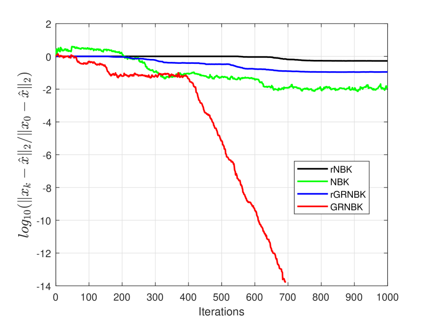
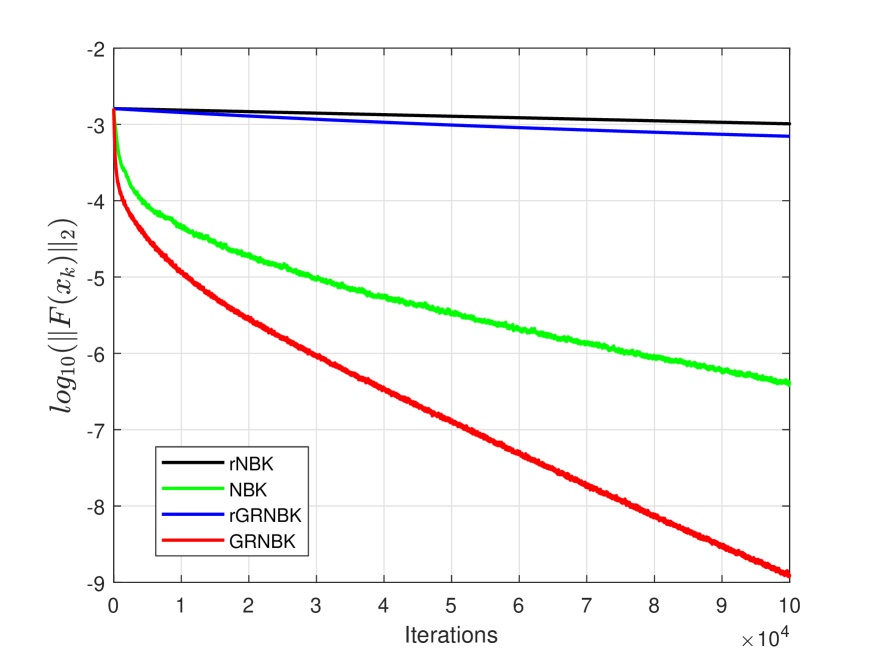
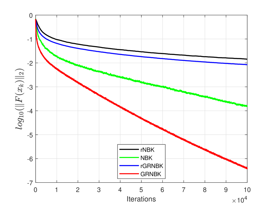
Figure 1: Convergence curves of residual versus iterations for Problem 5.1 with (n,d)=(500,100),s=10,λ=5formulae-sequence𝑛𝑑500100formulae-sequence𝑠10𝜆5(n,d)=(500,100),s=10,\lambda=5.

For a example, choosing A(i)𝒩(0,1)500×500similar-tosuperscript𝐴𝑖𝒩superscript01500500A^{(i)}\sim\mathcal{N}(0,1)^{500\times 500} for i=1,,100𝑖1100i=1,...,100, x^^𝑥\hat{x} with 101010 nonzero entries and λ=5𝜆5\lambda=5. In Figure 1, the curves of the norm of the residual versus the number of iteration steps and the solution error versus the number of iteration steps are plotted, respectively.

From Figure 1, it is seen that the GRNBK method clearly converges faster than the NBK method and the rGRNBK method converges faster than the rNBK method, which implies that the residual-based greedy strategies are effective and can greatly improve the convergence speed of nonlinear Bregman-Kaczmarz method. It is seen from Figure 1 that the convergence curves for the GRNBK method decreases much faster than those of its relaxed versions, which shows that the computation of the tk,φsubscript𝑡𝑘𝜑t_{k,\varphi} step size for GRNBK method pay off.

5.2 Linear systems on the probability simplex

Consider linear systems constrained to the probability simplex

find xΔd1, s.t. Ax=b.formulae-sequencefind 𝑥superscriptΔ𝑑1 s.t. 𝐴𝑥𝑏\text{find }x\in\Delta^{d-1},\text{ s.t. }Ax=b. (5.2)

That is, choosing Fi=ai,xbisubscript𝐹𝑖subscript𝑎𝑖𝑥subscript𝑏𝑖F_{i}=\langle a_{i},x\rangle-b_{i} and viewing C=Δd1={x0d:i=1dxi=1}𝐶superscriptΔ𝑑1conditional-set𝑥superscriptsubscriptabsent0𝑑superscriptsubscript𝑖1𝑑subscript𝑥𝑖1C=\Delta^{d-1}=\{x\in\mathbb{R}_{\geq 0}^{d}:\ \sum_{i=1}^{d}x_{i}=1\} as the additional constraint in problem (1.1). For NBK and GRNBK methods, the simplex-restricted negative entropy function from [7, Example 3.3] is used, which is given by

φ(x)={i=1dxilog(xi),xΔd1,+,otherwise.𝜑𝑥casessuperscriptsubscript𝑖1𝑑subscript𝑥𝑖subscript𝑥𝑖𝑥superscriptΔ𝑑1otherwise.\varphi(x)=\begin{cases}\sum_{i=1}^{d}x_{i}\log(x_{i}),&x\in\Delta^{d-1},\\ +\infty,&\text{otherwise.}\end{cases}

It is known from [7, Example 3.3] that φ𝜑\varphi is 111-strongly convex with respect to the 111-norm 1\|\cdot\|_{1}. Therefore, rNBK and rGRNBK methods with σ=1𝜎1\sigma=1 and =\|\cdot\|_{*}=\|\cdot\|_{\infty} are considered. Note that it holds fik(x)=aiksubscript𝑓subscript𝑖𝑘𝑥subscript𝑎subscript𝑖𝑘\nabla f_{i_{k}}(x)=a_{i_{k}} for all x𝑥x and βk=biksubscript𝛽𝑘subscript𝑏subscript𝑖𝑘\beta_{k}=b_{i_{k}} in NBK and GRNBK method. If problem (5.2) has a solution, then condition (3.3) is fulfilled in each step of NBK and GRNBK method, so these methods take always the stepsize tk=tk,φsubscript𝑡𝑘subscript𝑡𝑘𝜑t_{k}=t_{k,\varphi} from the exact Bregman projection.

Let the right-hand side be b=Ax^𝑏𝐴^𝑥b=A\hat{x} with the solution x^^𝑥\hat{x} drawn from the uniform distribution on the probability simplex Δd1superscriptΔ𝑑1\Delta^{d-1}. All iterations start from the center point x0=(1d,,1d)subscript𝑥01𝑑1𝑑x_{0}=(\frac{1}{d},...,\frac{1}{d}) and terminate when the norm of relative residual Axkb2/Ax0b2109subscriptnorm𝐴subscript𝑥𝑘𝑏2subscriptnorm𝐴subscript𝑥0𝑏2superscript109\left\|Ax_{k}-b\right\|_{2}/\left\|Ax_{0}-b\right\|_{2}\leq 10^{-9} or the number of iterations exceeds 10,000.

In the first setting, the matrix A𝐴A is generated from standard normal distribution. Specifically, A𝒩(0,1)n×dsimilar-to𝐴𝒩superscript01𝑛𝑑A\sim\mathcal{N}(0,1)^{n\times d} with (n,d)=(400,300)𝑛𝑑400300(n,d)=(400,300) in the overdetermined case and (n,d)=(300,400)𝑛𝑑300400(n,d)=(300,400) in the underdetermined case, respectively.

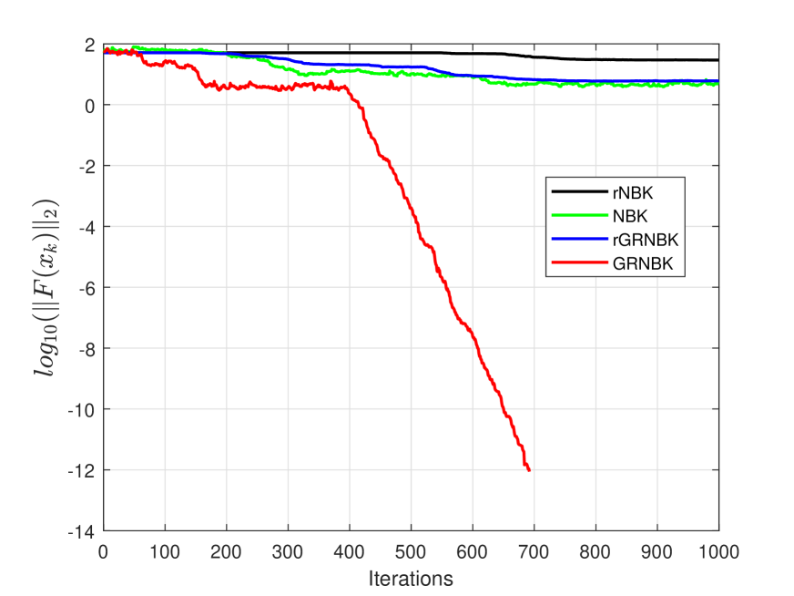
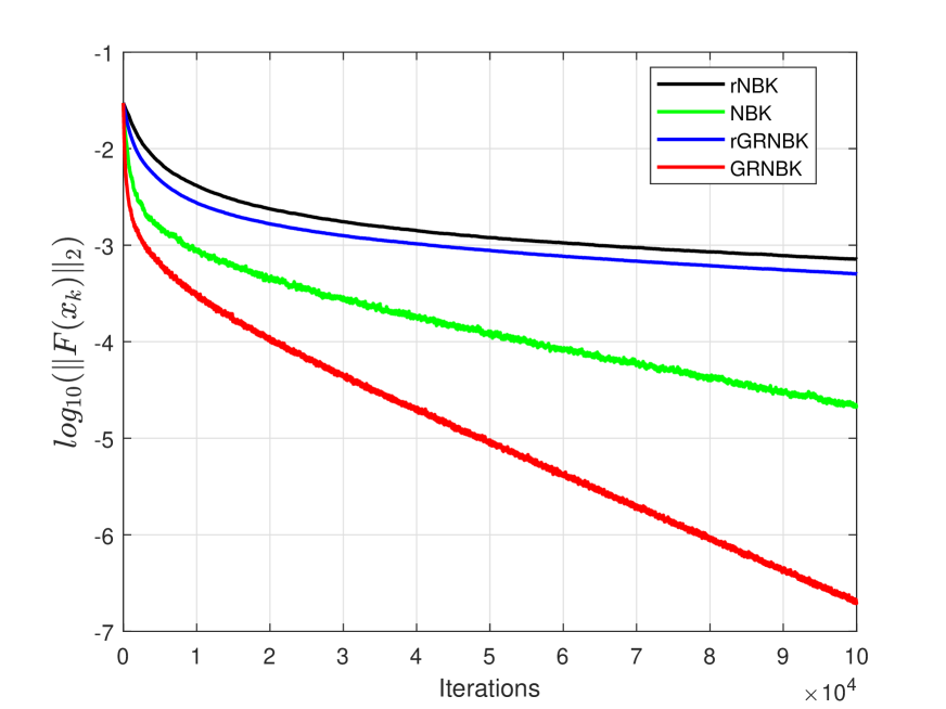
From Figure 2, it is seen that the GRNBK method converges faster than NBK method and the rGRNBK method converges faster than rNBK method both in the overdetermined and underdetermined case, which shows the advantage of the greedy strategy.
Refer to caption
Refer to caption
Figure 2: Convergence curves of residual versus iterations for Problem 5.2 with Left: A𝒩(0,1)400×300similar-to𝐴𝒩superscript01400300A\sim\mathcal{N}(0,1)^{400\times 300} and Right: A𝒩(0,1)300×400similar-to𝐴𝒩superscript01300400A\sim\mathcal{N}(0,1)^{300\times 400}.

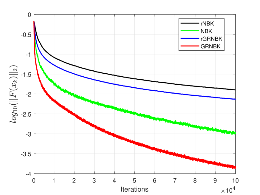
In the second setting, to study the impact of the distribution of entries of A𝐴A on convergence quality of the methods, the tested matrix A𝐴A is generated from uniformly distributed entries A𝒰([0,1])n×dsimilar-to𝐴𝒰superscript01𝑛𝑑A\sim\mathcal{U}([0,1])^{n\times d} and A𝒰([0.9,1])n×dsimilar-to𝐴𝒰superscript0.91𝑛𝑑A\sim\mathcal{U}([0.9,1])^{n\times d} with (n,d)=(300,400)𝑛𝑑300400(n,d)=(300,400), respectively. From Figure 3, it is seen that the redundant rows of the matrix A𝐴A don not deteriorate the convergence of the GRNBK method.
Refer to caption
Refer to caption
Figure 3: Convergence curves of residual versus iterations for Problem 5.2 with Left: A𝒰([0,1])300×400similar-to𝐴𝒰superscript01300400A\sim\mathcal{U}([0,1])^{300\times 400} and Right: A𝒰([0.9,1])300×400similar-to𝐴𝒰superscript0.91300400A\sim\mathcal{U}([0.9,1])^{300\times 400}.

5.3 Left stochastic decomposition

Consider the left stochastic decomposition problem formulated as follows:

find XLr×m, s.t. XTX=A,formulae-sequencefind 𝑋superscript𝐿𝑟𝑚 s.t. superscript𝑋𝑇𝑋𝐴\text{find }X\in L^{r\times m},\text{ s.t. }X^{T}X=A, (5.3)

where

Lr,m={P0r×m:PT\vmathbb1r=\vmathbb1m}superscript𝐿𝑟𝑚conditional-set𝑃subscriptsuperscript𝑟𝑚absent0superscript𝑃𝑇\vmathbbsubscript1𝑟\vmathbbsubscript1𝑚L^{r,m}=\big{\{}P\in\mathbb{R}^{r\times m}_{\geq 0}:P^{T}\vmathbb{1}_{r}=\vmathbb{1}_{m}\}

is the set of left stochastic matrices and Ar×m𝐴superscript𝑟𝑚A\in\mathbb{R}^{r\times m} is a given nonnegative matrix. The problem is equivalent to the so-called soft-K-means problem and hence has applications in clustering [1]. Regarding (5.3) as an instance of problem (1.1) with component equations

Fi,j(X)=X:,i,X:,jAi,j=0,i=1,,r,j=1,,mformulae-sequencesubscript𝐹𝑖𝑗𝑋subscript𝑋:𝑖subscript𝑋:𝑗subscript𝐴𝑖𝑗0formulae-sequence𝑖1𝑟𝑗1𝑚F_{i,j}(X)=\langle X_{:,i},X_{:,j}\rangle-A_{i,j}=0,\qquad i=1,...,r,\ j=1,...,m

and C=Lr×m(Δr1)m𝐶superscript𝐿𝑟𝑚superscriptsuperscriptΔ𝑟1𝑚C=L^{r\times m}\cong\left(\Delta^{r-1}\right)^{m}, where X:,isubscript𝑋:𝑖X_{:,i} represents the i𝑖ith column of X𝑋X.

For NBK and GRNBK method, the distance generating function is chosen from [7, Example 3.4] with the simplex-restricted negative entropy φi=φsubscript𝜑𝑖𝜑\varphi_{i}=\varphi from see [7, Example 3.3]. Since Fi,jsubscript𝐹𝑖𝑗F_{i,j} depends on at most two columns of X𝑋X, NBK and GRNBK method act on Δr1superscriptΔ𝑟1\Delta^{r-1} or Δr1×Δr1superscriptΔ𝑟1superscriptΔ𝑟1\Delta^{r-1}\times\Delta^{r-1} in each step. Therefore, the steps from [7, Example 3.3] is adopted in the first case, and from [7, Example 3.5] is used in the second case. Let A=X^TX^𝐴superscript^𝑋𝑇^𝑋A=\hat{X}^{T}\hat{X} and the columns of X^^𝑋\hat{X} be sampled according to the uniform distribution on Δr1superscriptΔ𝑟1\Delta^{r-1}. All iterations terminate when the norm of relative residual F(Xk)2105subscriptnorm𝐹subscript𝑋𝑘2superscript105\left\|F(X_{k})\right\|_{2}\leq 10^{-5} or the number of iterations exceeds 300,000.

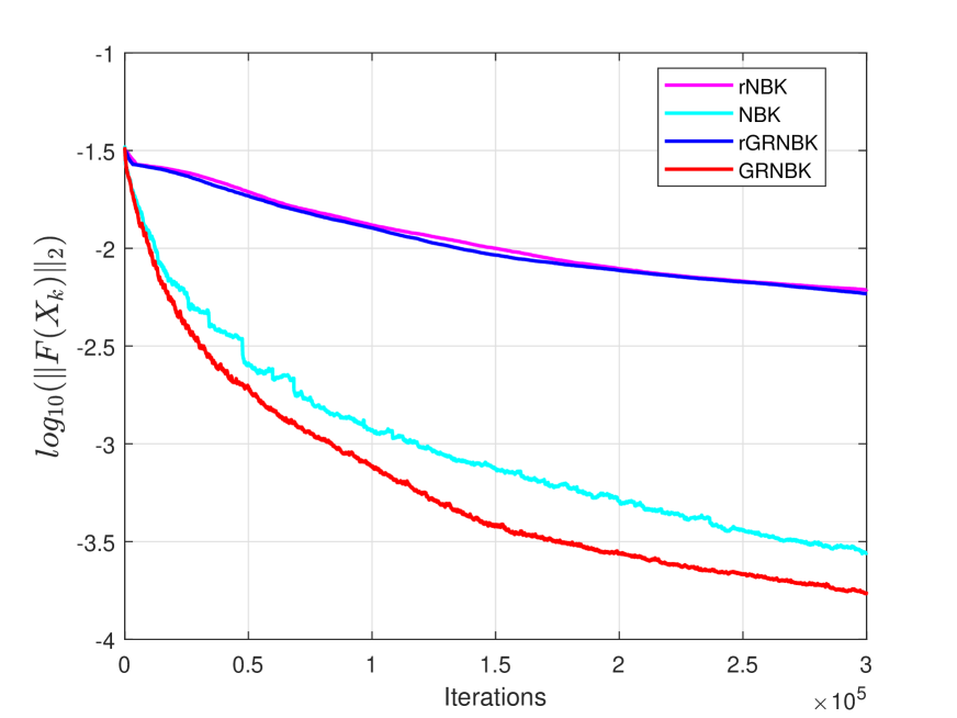
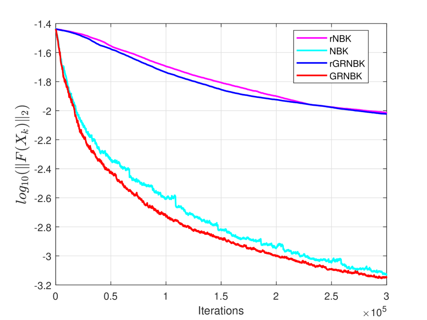
From Figure 4, it is shown that the GRNBK method has the fastest convergence speed among all methods, which indicates the efficiency of the greedy strategy.
Refer to caption
Refer to caption
Figure 4: Convergence curves of residual versus iterations for Problem 5.3 with Left: r=100,m=90formulae-sequence𝑟100𝑚90r=100,m=90 and Right: r=90,m=100formulae-sequence𝑟90𝑚100r=90,m=100.

6 Conclusions

In this paper, a greedy randomized nonlinear Bregman-Kaczmarz method and its relaxed version are presented for the solution of constrained nonlinear systems. The convergence theory of the greedy randomized nonlinear Bregman-Kaczmarz method and its relaxed version are studied under the classical local tangential cone conditions. Numerical experiments by considering different constraints demonstrate the efficiency and robustness of the proposed method, which has a faster convergence speed than existing nonlinear Bregman-Kaczmarz methods. In addition, some acceleration strategies for nonlinear Kaczmarz methods, such as averaging and sketching can be integrated into our methods. We leave these valuable topics to future work.

Acknowledgements Not Applicable.

Author Contributions All the authors contributed to the study conception, design and approval of the final manuscript.

Funding This work was supported by National Natural Science Foundation of China (No. 11971354).

Availability of supporting data No data was used for the research described in the article.

Declarations

Ethical Approval Not Applicable.

Competing Interests The authors declare that they have no conflict of interest.

References

  • [1] Raman Arora, Maya R Gupta, Amol Kapila, and Maryam Fazel. Similarity-based Clustering by Left-Stochastic Matrix Factorization. Journal of Machine Learning Research, 14(7):1715–1746, 2013.
  • [2] Zhong-Zhi Bai and Wen-Ting Wu. On greedy randomized augmented Kaczmarz method for solving large sparse inconsistent linear systems. SIAM Journal on Scientific Computing, 43(6):A3892–A3911, 2021.
  • [3] Heinz H Bauschke and Patrick L Combettes. Iterating Bregman retractions. SIAM Journal on Optimization, 13(4):1159–1173, 2003.
  • [4] Inderjit S Dhillon and Joel A Tropp. Matrix nearness problems with Bregman divergences. SIAM Journal on Matrix Analysis and Applications, 29(4):1120–1146, 2008.
  • [5] Albert Fannjiang and Thomas Strohmer. The numerics of phase retrieval. Acta Numerica, 29:125–228, 2020.
  • [6] Guang-Yu Gao, Bo Han, and Shan-Shan Tong. A projective two-point gradient Kaczmarz iteration for nonlinear ill-posed problems. Inverse Problems, 37(7):075007, 2021.
  • [7] Robert Gower, Dirk A Lorenz, and Maximilian Winkler. A Bregman–Kaczmarz method for nonlinear systems of equations. Computational Optimization and Applications, 87(3):1059–1098, 2024.
  • [8] Jamie Haddock and Anna Ma. Greed works: An improved analysis of sampling Kaczmarz–Motzkin. SIAM Journal on Mathematics of Data Science, 3(1):342–368, 2021.
  • [9] Benjamin Jarman, Yotam Yaniv, and Deanna Needell. Online signal recovery via heavy ball Kaczmarz. 1:276–280, 2022.
  • [10] Chao-Yue Liu, Li-Bin Zhu, and Mikhail Belkin. Loss landscapes and optimization in over-parameterized non-linear systems and neural networks. Applied and Computational Harmonic Analysis, 59:85–116, 2022.
  • [11] Dirk A Lorenz, Frank Schopfer, and Stephan Wenger. The linearized Bregman method via split feasibility problems: analysis and generalizations. SIAM Journal on Imaging Sciences, 7(2):1237–1262, 2014.
  • [12] Frank Schöpfer and Dirk A Lorenz. Linear convergence of the randomized sparse Kaczmarz method. Mathematical Programming, 173:509–536, 2019.
  • [13] Qi-Feng Wang, Wei-Guo Li, Wen-Di Bao, and Xing-Qi Gao. Nonlinear Kaczmarz algorithms and their convergence. Journal of Computational and Applied Mathematics, 399:113720, 2022.
  • [14] A-Qin Xiao and Jun-Feng Yin. On averaging block Kaczmarz methods for solving nonlinear systems of equations. Journal of Computational and Applied Mathematics, 451:116041, 2024.
  • [15] A-Qin Xiao, Jun-Feng Yin, and Ning Zheng. On fast greedy block Kaczmarz methods for solving large consistent linear systems. Computational and Applied Mathematics, 42(3):119, 2023.
  • [16] Rui Yuan, Alessandro Lazaric, and Robert M Gower. Sketched Newton–Raphson. SIAM Journal on Optimization, 32(3):1555–1583, 2022.
  • [17] Ya-Xiang Yuan. Recent advances in numerical methods for nonlinear equations and nonlinear least squares. Numerical algebra, control and optimization, 1(1):15–34, 2011.
  • [18] Fei-Yu Zhang, Wen-Di Bao, Wei-Guo Li, and Qin Wang. On sampling Kaczmarz–Motzkin methods for solving large-scale nonlinear systems. Computational and Applied Mathematics, 42(3):126, 2023.
  • [19] Jian-Hua Zhang, Yu-Qing Wang, and Jing Zhao. On maximum residual nonlinear Kaczmarz-type algorithms for large nonlinear systems of equations. Journal of Computational and Applied Mathematics, 425:115065, 2023.
  • [20] Yan-Jun Zhang, Han-Yu Li, and Ling Tang. Greedy randomized sampling nonlinear Kaczmarz methods. Calcolo, 61(2):25, 2024.