Proper Implicit Discretization of the Super-Twisting Controller—without and with Actuator Saturation

Abstract

The discrete-time implementation of the super-twisting sliding mode controller for a plant with disturbances with bounded slope, zero-order hold actuation, and actuator constraints is considered. Motivated by restrictions of existing implicit or semi-implicit discretization variants, a new proper implicit discretization for the super-twisting controller is proposed. This discretization is then extended to the conditioned super-twisting controller, which mitigates windup in presence of actuator constraints by means of the conditioning technique. It is proven that the proposed controllers achieve best possible worst-case performance subject to similarily simple stability conditions as their continuous-time counterparts. Numerical simulations and comparisons demonstrate and illustrate the results.

,

1 Introduction

Sliding mode control (SMC) is a robust control technique for systems that contain uncertainties. In continuous time, SMC manages to completely reject disturbances that fulfill certain requirements after a finite convergence time, see e.g. (Shtessel et al., 2013). However, implementing SMC in practice is not straightforward and often leads to chattering due to discretization and measurement noise, as shown by Levant (2011). One approach to reduce chattering effects is higher-order SMC. A popular second-order sliding mode controller that rejects disturbances with bounded derivative is the Super-Twisting Controller (STC) introduced by Levant (1993).

In (Koch and Reichhartinger, 2019) the authors proposed a discretization of the super-twisting algorithm, i.e., the closed-loop system with the STC, on the basis of an eigenvalue mapping from continuous- to discrete-time. They applied an implicit and an exact mapping yielding an implicit and a matching discretization, respectively, mitigating chattering to some extent. Hanan et al. (2021) proposed a low-chattering discretization of SMC that is based on an explicit discretization and significantly reduces chattering effects. An implicit discretization of the STC that avoids discretization chattering based on ideas from (Acary and Brogliato, 2010) was proposed by Brogliato et al. (2020). Another discrete-time representation of the STC that is based on a semi-implicit discretization and also avoids discretization chattering was developed by Xiong et al. (2022). More recently, a modified implicitly discretized STC was proposed by Andritsch et al. (2023), where the authors also performed detailed comparisons between existing discretizations of the STC.

Apart from the need for a discrete-time implementation, real-life plants in practice also often have limitations regarding the control input that can be applied. The STC includes controller dynamics, which in combination with a saturated control input can lead to windup effects in the controller. This may diminish the control performance, e.g. by increased convergence times or large overshoot of the system states. A method to avoid windup is the so-called conditioning technique by Hanus et al. (1987). For the case of saturated control, the conditioning technique was applied to the continuous-time STC by Seeber and Reichhartinger (2020). Reichhartinger et al. (2023) applied anti-windup schemes directly to discrete-time realizations of the STC, e.g. (Koch and Reichhartinger, 2019). In Yang et al. (2023) the authors applied the semi-implicit discretization by Xiong et al. (2022) to the conditioned STC, obtaining a discrete-time implementation of the STC with windup mitigation.

Compared to the continuous-time STC, the discussed discrete-time implementations without and with actuator saturation exhibit various restrictions. In particular, the discrete-time STC by Brogliato et al. (2020) can handle a smaller class of disturbances; this will be formally demonstrated later on and is also shown in the comparative results in (Andritsch et al., 2023). The latter comparisons also show that the discretization by Xiong et al. (2022) is harder to tune, because certain parameter selections result in a significantly increased convergence time. These shortcomings are avoided by Andritsch et al. (2023); however, their discretization lacks a proof of global closed-loop stability in the presence of a disturbance, as do the discrete-time controllers with saturation studied in (Reichhartinger et al., 2023). The conditioned discrete-time STC by Yang et al. (2023), finally, has similar drawbacks as the unconditioned semi-implicitly discretized STC by Xiong et al. (2022) and additionally does not necessarily achieve the best possible worst-case error, as shown in (Seeber, 2024).

The present paper derives a novel discretization of the STC that does not have the disadvantages of previously proposed discretizations and is shown to yield the best possible worst-case control error. Furthermore, a complete stability proof and simple stability conditions are provided, extending those given by Brogliato et al. (2020), in addition to extending the class of perturbations. For the case of saturated actuation, the conditioning technique is applied to the proposed discrete-time STC, yielding an implicit discretization of the conditioned STC. Also for this case, stability conditions are derived that are very similar to those obtained in (Seeber and Reichhartinger, 2020) for the continuous-time case. Moreover, explicit controller realizations are derived, in a similar fashion as recently noted by Brogliato (2023) for the first-order controllers by Haddad and Lee (2020).

The paper is structured as follows. Section 2 introduces and motivates the problem statement based on existing approaches in literature. Sections 3 and 4 present the main results: implementations and formal guarantees for the implicit STC in absence and presence of actuator saturation, respectively. Sections 5 and 6 then present the corresponding derivations, with the derivation of explicit control laws being contained in the former and the stability analysis being performed in the latter. Section 7 demonstrates the effectiveness of the proposed discrete-time controllers by means of simulations and comparisons. Section 8, finally, concludes the paper.

Notation: $\mathbb{R}$, $\mathbb{R}_{\geq 0}$, $\mathbb{R}_{>0}$, $\mathbb{Z}$, $\mathbb{N}$, and $\mathbb{N}_{0}$ denote reals, nonnegative reals, positive reals, integers, positive integers, and nonnegative integers. For $y,p\in\mathbb{R}$, $p\neq 0$, the abbreviation $\left\lfloor y\right\rceil^{p}=\left\lvert y\right\rvert^{p}\operatorname{sign}(y)$ is used with $\operatorname{sign}(0)=0$, and $\left\lfloor y\right\rceil^{0}$ denotes the set-valued sign function defined as $\left\lfloor y\right\rceil^{0}=\{\operatorname{sign}(y)\}$ for $y\neq 0$ and $\left\lfloor 0\right\rceil^{0}=[-1,1]$. The real-valued mod-operator $a\text{ mod }b=r$, where $a,b\in\mathbb{R}$, $b\neq 0$, is the unique $r\in[0,|b|)$ fulfilling $a=r+kb$ with $k\in\mathbb{Z}$. The set of all subsets of a set $\mathcal{S}$ is denoted by $2^{\mathcal{S}}$.

2 Motivation and Problem Statement

2.1 Zero-Order Hold Sampled Sliding Mode Control

Consider a scalar sliding variable $x\in\mathbb{R}$ governed by

$$\dot{x}=u+w$$ (1)

with a control input $u:\mathbb{R}_{\geq 0}\to\mathbb{R}$ generated by a zero-order hold element with sampling time $T\in\mathbb{R}_{>0}$ from a control input sequence $(u_{k})$, $k\in\mathbb{N}_{0}$, according to

$$u(t)=u_{k}\qquad\text{for $t\in[kT,(k+1)T)$}$$ (2)

and an unknown disturbance $w:\mathbb{R}_{\geq 0}\to\mathbb{R}$ whose slope and amplitude are bounded by $|\dot{w}(t)|\leq L\in\mathbb{R}_{\geq 0}$ almost everywhere and $|w|\leq W\in\mathbb{R}_{\geq 0}\cup\{\infty\}$ for all $t\in\mathbb{R}_{\geq 0}$. The control goal is to drive the sliding variable to a vicinity of the origin that is as small as possible, considering that the disturbance is unknown. To that end, consider the samples $x_{k}=x(kT)$ with $k\in\mathbb{N}_{0}$ and define

$$w_{k}=\frac{1}{T}\int_{kT}^{(k+1)T}w(\tau)\,\mathrm{d}\tau$$ (3)

to obtain the zero-order hold discretization of (1) as

$$x_{k+1}=x_{k}+T(u_{k}+w_{k}).$$ (4)

It is easy to verify that the disturbance $w_{k}$ therein satisfies $|w_{k+1}-w_{k}|\leq LT$ and $|w_{k}|\leq W$ for all $k\in\mathbb{N}_{0}$.

The following motivating proposition shows a lower bound on the worst-case disturbance rejection. It is proven in Appendix A.1.

Proposition 1.

Let $L\in\mathbb{R}_{\geq 0}$, $T\in\mathbb{R}_{>0}$, $W\geq\frac{3LT}{2}$ and consider the continuous-time plant (1) with zero-order hold input (2) and sampled output $x_{k}=x(kT)$. Then, for every initial condition $x_{0}\in\mathbb{R}$, for every causal control law, i.e., for every sequence $(h_{k})$ of functions $h_{k}:\mathbb{R}^{k+1}\to\mathbb{R}$ such that $u_{k}=h_{k}(x_{k},x_{k-1},\ldots,x_{0}),$ and for every $K\in\mathbb{N}$ there exists a Lipschitz continuous disturbance $w:\mathbb{R}_{\geq 0}\to\mathbb{R}$ satisfying $|w(t)|\leq W$ and $|\dot{w}(t)|\leq L$ almost everywhere such that

$$\sup_{t\geq KT}|x(t)|\geq\sup_{k\geq K}|x_{k}|\geq LT^{2}$$ (5)

holds for the corresponding closed-loop trajectory.

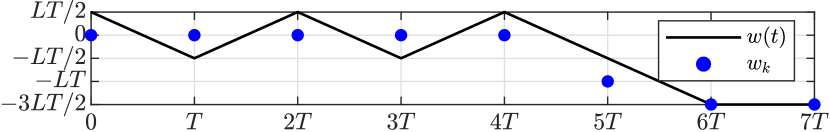
Figure 1: Example for a disturbance signal $w(t)$ and corresponsing $w_{k}$ limiting the worst-case error as in Proposition 1.

Remark 2.

Fig. 1 shows a disturbance $w(t)$ obtained from the proof of Proposition 1 with $K=4$ and corresponding $w_{k}$ that leads to the state $x_{k}$ reaching the best possible worst-case bound $LT^{2}$.

In continuous time, a well-known sliding mode controller for the plant (1) is the super-twisting controller

$$u =-k_{1}\left\lfloor x\right\rceil^{\frac{1}{2}}+v, \dot{v} =-k_{2}\operatorname{sign}(x)$$ (6)

proposed by Levant (1993), with positive parameters $k_{1},k_{2}$ and trajectories understood in the sense of Filippov (1988). The goal of the present paper is to obtain a discrete-time implementation of this controller for the sampled control problem such that

• the optimal worst-case performance from Proposition 1 is attained in finite time, i.e., such that $|x(t)|\leq LT^{2}$ holds after a finite time, and

• this optimal performance is maintained also in the presence of actuator saturation while, additionally, controller windup is mitigated.

Arguably, the most promising approaches for achieving these goals are the implicit or semi-implicit discretization techniques due to Brogliato et al. (2020); Xiong et al. (2022) in combination with the conditioning technique for windup mitigation proposed by Hanus et al. (1987). In the following, the state-of-the-art solutions in that regard are discussed to motivate the present work.

2.2 State-of-the-Art Implicit Super-Twisting Control

Brogliato et al. (2020) propose an implicit super-twisting controller given by the generalized equations

$$u_{k} =-k_{1}\left\lfloor x_{k}+Tu_{k}\right\rceil^{\frac{1}{2}}+v_{k+1}$$ (7a)

$$v_{k+1} \in v_{k}-k_{2}T\left\lfloor x_{k}+Tu_{k}\right\rceil^{0}.$$ (7b)

However, they perform the discretization considering only the unperturbed case. As a consequence, this controller—unlike the continuous-time super-twisting controller—is not capable of rejecting unbounded disturbances with bounded slope. To see this, note that with abbreviations $w_{-2}:=w_{0}$, $w_{-1}:=w_{0}$ the trajectory $x_{k}=Tw_{k-1},u_{k}=-w_{k-1},v_{k}=-w_{k-2}$ is always a solution of the closed loop (4), (7), provided that $k_{2}>L$. As a consequence, the controller (7) can only guarantee that $|x_{k}|\leq WT$ holds after a finite number of steps.

2.3 Semi-Implicit Conditioned Super-Twisting Control

Consider now the case of actuator saturation, i.e., the case that the control input $u$ is bounded by some control input bound $U\in\mathbb{R}_{>0}$ with $U>W$. In this case, the classical super-twisting controller (6) may suffer from a windup effect that deteriorates control performance.

A continuous-time control law that mitigates this windup effect is the conditioned super-twisting controller proposed by Seeber and Reichhartinger (2020). Its control law is obtained by applying the conditioning technique by Hanus et al. (1987) to (6) and is given by

$$\bar{u} =-k_{1}\left\lfloor x\right\rceil^{\frac{1}{2}}+v$$ (8a)

$$u =\operatorname{sat}_{U}(\bar{u}):=\begin{cases}\bar{u}&|\bar{u}|\leq U\\ U\operatorname{sign}(\bar{u})&|\bar{u}|>U\end{cases}$$ (8b)

$$\dot{v} =-k_{2}\operatorname{sign}(v-u).$$ (8c)

Yang et al. (2023) propose a semi-implicit discretization of this controller. However, as shown in (Seeber, 2024), that discretization may suffer from limit cycles which deteriorate the achievable performance compared to the unsaturated case.

The present paper proposes new, proper implicit discretizations of both, the super-twisting controller and the conditioned super-twisting controller, such that the best possible worst-case performance shown in Proposition 1 is achieved in either case.

3 Implicit Super-Twisting Control
without Actuator Saturation

In the following, a new implicit discretization of the super-twisting controller with best possible worst-case disturbance rejection is derived. First, note that (7) drives the modified sliding variable $\tilde{x}_{k}=x_{k}-Tw_{k-1}$ to zero, i.e., the variable $\tilde{x}_{k}$ defines the discrete-time sliding mode. This variable satisfies

$$\tilde{x}_{k+1} =x_{k}+Tu_{k}$$ (9a)

$$=\tilde{x}_{k}+T(u_{k}+w_{k-1}).$$ (9b)

In (Brogliato et al., 2020), this variable was chosen such that (9a) does not depend on $w_{k}$, because otherwise the unknown quantity $w_{k}$ would be needed to compute $u_{k}$.

From (9b), one may see that $v_{k+1}$ in (7a) eventually compensates for $w_{k-1}$. Using this intuition and the fact that the difference of two successive disturbance values satisfies $|w_{k-1}-w_{k-2}|\leq LT$, an alternative modified sliding variable is proposed as

$$z_{k} =x_{k}-T(w_{k-2}+v_{k})-T(w_{k-1}-w_{k-2})$$

$$=x_{k}-T(w_{k-1}+v_{k}).$$ (10)

If $z_{k}$ and $v_{k}+w_{k-2}$ are driven to zero, then $x_{k}$ satisfies the desired bound $|x_{k}|\leq T|w_{k-1}-w_{k-2}|\leq LT^{2}$. By combining (4) and (3) to

$$z_{k+1} =x_{k}+T(u_{k}-v_{k+1})$$ (11a)

$$=z_{k}+T(u_{k}+w_{k-1}+v_{k}-v_{k+1}),$$ (11b)

one can see that the proposed modified sliding variable $z_{k}$ also has the property that the prediction (11a) does not depend on the unknown quantity $w_{k}$. The controller (7) contains the term $v_{k+1}$ to compensate for $w_{k-1}$ in  (9b). This suggests that the control law that drives $z_{k}$ in (11b) to zero should contain the term $2v_{k+1}-v_{k}$ to compensate for $w_{k-1}+v_{k}-v_{k+1}$. The proposed proper implicit discretization of the super-twisting controller without actuator saturation is hence given by

$$u_{k} =-k_{1}\left\lfloor z_{k+1}\right\rceil^{\frac{1}{2}}+2v_{k+1}-v_{k}$$ (12a)

$$v_{k+1} \in v_{k}-Tk_{2}\left\lfloor z_{k+1}\right\rceil^{0}.$$ (12b)

The next two theorems show how to implement this control law in explicit form and give closed-loop stability conditions. Their proofs are given in Sections 5.1 and 6.1.

Theorem 3.

Let $k_{1},k_{2},T\in\mathbb{R}_{>0}$ and define the abbreviation $\lambda=k_{2}-\frac{k_{1}^{2}}{4}$. Then, the explicit form of the implicit control law (12), i.e., the unique solution $u_{k},v_{k+1}$ of the system of generalized equations (11a) and (12), is given by

$$u_{k}=\begin{cases}v_{k}-\left(2\lambda T+k_{1}\sqrt{|x_{k}|-\lambda T^{2}}\right)\operatorname{sign}(x_{k})&\frac{|x_{k}|}{T^{2}}>k_{2}\\ v_{k}-\frac{2x_{k}}{T}&\frac{|x_{k}|}{T^{2}}\leq k_{2}\end{cases}$$ (13a)

$$v_{k+1}=\begin{cases}v_{k}-Tk_{2}\operatorname{sign}(x_{k})&\frac{|x_{k}|}{T^{2}}>k_{2}\\ v_{k}-\frac{x_{k}}{T}&\frac{|x_{k}|}{T^{2}}\leq k_{2}\end{cases}$$ (13b)

for every given $x_{k},v_{k}\in\mathbb{R}$.

Remark 4.

It is worth noting that the proposed explicit control law (13) coincides with the discrete-time controller proposed by Andritsch et al. (2023). However, the presented derivation provides an intuitive motivation that allows for a complete stability proof.

Remark 5.

It is remarkable that for $k_{1}=2\sqrt{k_{2}}$, the proposed implicit discretization of the super-twisting controller has the particularly simple form

$$u_{k}=-k_{1}\left\lfloor x_{k}\right\rceil^{\frac{1}{2}}+v_{k},\quad v_{k+1}=v_{k}-Tk_{2}\operatorname{sign}(x_{k})$$ (14)

for $|x_{k}|>k_{2}T^{2}$, which corresponds to the super-twisting controller with explicit Euler discretization. Also, it becomes a second-order dead-beat controller for ${|x_{k}|\leq k_{2}T^{2}}$ regardless of $k_{1}$.

Theorem 6.

Let $L\in\mathbb{R}_{\geq 0}$, $T\in\mathbb{R}_{>0}$ and consider the interconnection of the control law (13), the zero-order hold (2), and the continuous-time plant (1). Suppose that the disturbance $w:\mathbb{R}_{\geq 0}\to\mathbb{R}$ is Lipschitz continuous, fulfilling $|\dot{w}(t)|\leq L$ almost everywhere, and that the controller parameters $k_{1},k_{2}\in\mathbb{R}_{>0}$ satisfy

$$k_{1}>\sqrt{k_{2}+L},\qquad k_{2}>L.$$ (15)

Define $x_{k}=x(kT)$ and $w_{k}$ as in (3). Then, an integer $K$ exists such that $v_{k}=-w_{k-2}$, $x_{k}=T(w_{k-1}-w_{k-2})$ hold for all $k\geq K$, and $|x(t)|\leq LT^{2}$ holds for all $t\geq KT$.

4 Implicit Conditioned Super-Twisting Control with Actuator Saturation

In order to obtain an implicit discretization of the conditioned super-twisting controller, note that, in continuous time, its construction is based on the fact that in (8c)

$$\operatorname{sign}(v-u)=\operatorname{sign}(k_{1}\left\lfloor x\right\rceil^{\frac{1}{2}})=\operatorname{sign}(x)$$ (16)

holds for $k_{1}>0$ in the unsaturated case $u=\bar{u}$. Applying a similar modification to (12) yields the proposed implicit conditioned super-twisting controller as

$$\bar{u}_{k} =-k_{1}\left\lfloor z_{k+1}\right\rceil^{\frac{1}{2}}+2v_{k+1}-v_{k}$$ (17a)

$$u_{k} =\operatorname{sat}_{U}(\bar{u}_{k})$$ (17b)

$$v_{k+1} \in v_{k}-Tk_{2}\left\lfloor 2v_{k+1}-v_{k}-u_{k}\right\rceil^{0}.$$ (17c)

The next two theorems show how to implement this control law in explicit form and give closed-loop stability conditions. Their proofs are given in Sections 5.2 and 6.2.

Theorem 7.

Let $k_{1},k_{2},T,U\in\mathbb{R}_{>0}$ and define the abbreviation $\lambda=k_{2}-\frac{k_{1}^{2}}{4}$. Then, an explicit form of the implicit conditioned super-twisting controller (17), i.e., a solution $u_{k},v_{k+1}$ of the system of generalized equations (11a) and (17), is given by

$$\hat{u}_{k}=\begin{cases}v_{k}-\left(2\lambda T+k_{1}\sqrt{|x_{k}|-\lambda T^{2}}\right)\operatorname{sign}(x_{k})&\frac{|x_{k}|}{T^{2}}>k_{2}\\ v_{k}-\frac{2x_{k}}{T}&\frac{|x_{k}|}{T^{2}}\leq k_{2}\end{cases}$$ (18a)

$$u_{k}=\operatorname{sat}_{U}(\hat{u}_{k})$$ (18b)

$$v_{k+1}=\begin{cases}v_{k}-Tk_{2}\operatorname{sign}(v_{k}-u_{k})&|v_{k}-u_{k}|>2k_{2}T\\ \frac{v_{k}+u_{k}}{2}&|v_{k}-u_{k}|\leq 2k_{2}T\end{cases}$$ (18c)

for every given $x_{k},v_{k}\in\mathbb{R}$.

Remark 8.

Formally setting $U=\infty$ in (18) yields (13).

Remark 9.

Note that the auxiliary variable $\hat{u}_{k}$ in the explicit form (18) is not necessarily equal to the auxiliary variable $\bar{u}_{k}$ in the implicit form (17) when $\left\lvert u_{k}\right\rvert=U$.

Theorem 10.

Let $L,W\in\mathbb{R}_{\geq 0}$, $T\in\mathbb{R}_{>0}$. Consider the interconnection of the control law (18), the zero-order hold (2), and the continuous-time plant (1) with a bounded, Lipschitz continuous disturbance $w:\mathbb{R}_{\geq 0}\to\mathbb{R}$ satisfying $|\dot{w}(t)|\leq L$ and $|w(t)|\leq W$ almost everywhere. Suppose that the control input bound $U\in\mathbb{R}_{>0}$ and the parameters $k_{1},k_{2}\in\mathbb{R}_{>0}$ satisfy $U>W+k_{2}T$ and

$$k_{1}>\sqrt{2k_{2}\frac{U+W}{U-W-k_{2}T}},\qquad k_{2}>L.$$ (19)

Define $x_{k}=x(kT)$ and $w_{k}$ as in (3). Then, an integer $K$ exists such that $v_{k}=-w_{k-2}$, $x_{k}=T(w_{k-1}-w_{k-2})$ hold for all $k\geq K$, and $|x(t)|\leq LT^{2}$ holds for all $t\geq KT$.

5 Derivation of Explicit Control Laws

This section formally derives the explicit forms of the control laws in Sections 3 and 4.

5.1 Unsaturated Control Input

The explicit control law (13) of the proposed implicit super-twisting controller is obtained in a similar fashion as in (Brogliato et al., 2020), using the following auxiliary lemma. Its proof is given in Appendix A.2.

Lemma 11.

Let $k_{1},k_{2},T\in\mathbb{R}_{>0}$, define $\lambda=k_{2}-\frac{k_{1}^{2}}{4}$, and let $x_{k},v_{k}\in\mathbb{R}$. Then, the unique solution $z_{k+1}$ of (11a), (12) is given by

$$z_{k+1}=\begin{cases}\left(\sqrt{|x_{k}|-\lambda T^{2}}-\frac{Tk_{1}}{2}\right)^{2}\operatorname{sign}(x_{k})&|x_{k}|>k_{2}T^{2}\\ 0&|x_{k}|\leq k_{2}T^{2}.\end{cases}$$ (20)

Remark 12.

Alternatively, the framework of monotone operators and their resolvents (cf. Bauschke and Combettes, 2011, Chapter 23) could be used to solve for $z_{k+1}$ in (11a), (12). In this case, the resolvent has the same structure as obtained in (Mojallizadeh et al., 2021) for the implicit super-twisting differentiator.

Proof 5.1 (Proof of Theorem 3).

Using the unique solution $z_{k+1}$ from Lemma 11, distinguish the two cases in (20). In the first case, $\operatorname{sign}(z_{k+1})=\operatorname{sign}(x_{k})$ and (12b) yield (13b), and from (12a) one obtains

$$u_{k}-v_{k} =-k_{1}\left\lfloor z_{k+1}\right\rceil^{\frac{1}{2}}+2v_{k+1}-2v_{k}$$

$$=\left(\frac{Tk_{1}^{2}}{2}-k_{1}\sqrt{|x_{k}|-\lambda T^{2}}-2Tk_{2}\right)\operatorname{sign}(x_{k})$$

$$=-\left(2\lambda T+k_{1}\sqrt{|x_{k}|-\lambda T^{2}}\right)\operatorname{sign}(x_{k}).$$ (21)

In the second case, $0=z_{k+1}=x_{k}+T(v_{k+1}-v_{k})$ yields (13b), and (12a) yields $u_{k}=2v_{k+1}-v_{k}=v_{k}-\frac{2x_{k}}{T}$.

5.2 Saturated Control Input

Obtaining the explicit form of the implicit conditioned super-twisting controller (17) requires solving the system of generalized equations (11a), (17) containing the nonlinear saturation function. The following lemma reduces this problem to the solution of the unsaturated equations (11a), (12) with variables $z_{k+1},v_{k+1},u_{k}$ renamed to $\hat{z}_{k+1},\hat{v}_{k+1},\hat{u}_{k}$. The proof is in Appendix A.3.

Lemma 13.

Let $k_{1},k_{2},T,U\in\mathbb{R}_{>0}$ and $x_{k},v_{k}\in\mathbb{R}$. Consider the unique solution $\hat{u}_{k}$ of the system of generalized equations

$$\hat{z}_{k+1} =x_{k}+T(\hat{u}_{k}-\hat{v}_{k+1})$$ (22a)

$$\hat{u}_{k} =-k_{1}\left\lfloor\hat{z}_{k+1}\right\rceil^{\frac{1}{2}}+2\hat{v}_{k+1}-v_{k}$$ (22b)

$$\hat{v}_{k+1} \in v_{k}-Tk_{2}\left\lfloor\hat{z}_{k+1}\right\rceil^{0}.$$ (22c)

Then, $u_{k}=\operatorname{sat}_{U}(\hat{u}_{k})$ is a solution of the generalized system of equations (11a), (17).

Proof 5.2 (Proof of Theorem 7).

Apply Theorem 3 to system (22) to see from (13a) that (18a) is its unique solution. Lemma 13 then yields (18b). To show, finally, that (18c) is the unique solution of (17c), define $a_{k+1}=2v_{k+1}-v_{k}-u_{k}$, $b_{k}=v_{k}-u_{k}$ and rewrite (17c) as $a_{k+1}\in b_{k}-2Tk_{2}\left\lfloor a_{k+1}\right\rceil^{0}.$ Its unique solution is $a_{k+1}=b_{k}-2Tk_{2}\operatorname{sign}(b_{k})$ for $|b_{k}|>2k_{2}T$ and $a_{k+1}=0$ otherwise, from which (18c) follows.

6 Stability Analysis

The stability analysis is performed by proving forward invariance and finite-time attractivity of certain sets according to the following definition.

Definition 14.

Consider trajectories of a discrete-time system, i.e., sequences $(\mathbf{x}_{k})$ with $\mathbf{x}_{k}\in\mathbb{R}^{n}$. A set $\Omega\subseteq\mathbb{R}^{n}$ is called

• forward invariant along the trajectories, if for all trajectories $(\mathbf{x}_{k})$, $\mathbf{x}_{k}\in\Omega$ implies $\mathbf{x}_{k+1}\in\Omega$ for all $k\in\mathbb{N}_{0}$

• finite-time attractive along the trajectories, if for each trajectory $(\mathbf{x}_{k})$, there exists $K\in\mathbb{N}_{0}$ depending only on $\mathbf{x}_{0}$ such that $\mathbf{x}_{k}\in\Omega$ holds for all $k\geq K$.

6.1 Unsaturated Control Input

Consider the closed loop formed by interconnecting the plant (4) without actuator constraints and the proposed control law (12). To investigate its stability properties, consider the state variables $z_{k}$ and $q_{k}$ defined as, cf. (3),

$$z_{k}=x_{k}-T(w_{k-1}+v_{k}),\quad q_{k}=v_{k}+w_{k-2},$$ (23)

with the definition $w_{-k}:=w_{0}$ for $k\in\mathbb{N}$. According to (11b) and (12), these are governed by

$$z_{k+1} =z_{k}-Tk_{1}\left\lfloor z_{k+1}\right\rceil^{\frac{1}{2}}+Tq_{k+1}$$ (24a)

$$q_{k+1} \in q_{k}-Tk_{2}\left\lfloor z_{k+1}\right\rceil^{0}+T\delta_{k+1}$$ (24b)

with the abbreviation

$$\delta_{k}=\frac{w_{k-2}-w_{k-3}}{T}\quad\text{satisfying $|\delta_{k}|\leq L$.}$$ (24c)

Similar to (Brogliato et al., 2020), the stability analysis is based on the fact that (24) may be interpreted as the implicit discretization of the continuous-time closed-loop system, understood in the sense of Filippov (1988),

$$\dot{z} =-k_{1}\left\lfloor z\right\rceil^{\frac{1}{2}}+q$$ (25a)

$$\dot{q} =-k_{2}\operatorname{sign}(z)+\delta,\qquad\left\lvert\delta\right\rvert\leq L$$ (25b)

obtained by applying the continuous-time super-twisting controller (6) to (1) with $z=x$ and $q=v+w$.

Stability properties of the discrete-time closed loop may hence be analyzed using a Lyapunov function that is quasiconvex, i.e., that has convex sublevel sets. The next lemma, proven in Appendix A.4, generalizes (Brogliato et al., 2020, Lemma 5) to quasiconvex Lyapunov functions which are only locally Lipschitz continuous and may hence be analyzed using Clarke’s generalized gradient, cf. e.g. (Polyakov and Fridman, 2014, Section 5.4).

Lemma 15.

Let $\mathcal{F}:\mathbb{R}^{n}\to 2^{\mathbb{R}^{n}}$ be upper semicontinuous and $\mathcal{F}(\mathbf{x})$ be nonempty and compact for all $\mathbf{x}\in\mathbb{R}^{n}$. Let $V:\mathbb{R}^{n}\to\mathbb{R}_{\geq 0}$ be continuous, quasiconvex, positive definite, and locally Lipschitz continuous on $\mathbb{R}^{n}\setminus\{\bm{0}\}$. Denote by $\partial V:\mathbb{R}^{n}\setminus\{\bm{0}\}\to 2^{\mathbb{R}^{n}}$ its Clarke generalized gradient. Suppose that, for each $\mathbf{x}\in\mathbb{R}^{n}\setminus\{\bm{0}\}$,

$$\max_{\begin{subarray}{c}\mathbf{h}\in\mathcal{F}(\mathbf{x})\\ \bm{\zeta}\in\partial V(\mathbf{x})\end{subarray}}\bm{\zeta}^{\mathrm{T}}\mathbf{h}<0$$ (26)

holds. Then, for each $T\in\mathbb{R}_{>0}$ there exists a negative definite, upper semicontinuous function $Q_{T}:\mathbb{R}^{n}\to\mathbb{R}_{\geq 0}$ such that $V(\mathbf{x}_{k+1})-V(\mathbf{x}_{k})\leq Q_{T}(\mathbf{x}_{k+1})$ holds for all solutions of the inclusion $\mathbf{x}_{k+1}\in\mathbf{x}_{k}+T\mathcal{F}(\mathbf{x}_{k+1})$.

Remark 16.

Condition (26) essentially means that $\dot{V}$ is negative along trajectories of the system $\dot{\mathbf{x}}\in\mathcal{F}(\mathbf{x})$, i.e., that $V$ is a strict Lyapunov function for that system.

The Lyapunov function from (Seeber and Horn, 2017) is now used; it is shown to be quasiconvex in the following lemma, which is proven in Appendix A.5.

Lemma 17.

Let $L\in\mathbb{R}_{\geq 0}$, $k_{1},k_{2}\in\mathbb{R}_{>0}$ and consider the function $V_{\alpha}:\mathbb{R}^{2}\to\mathbb{R}$ defined as

$$V_{\alpha}(z,q)=\begin{cases}2\sqrt{q^{2}+3\alpha^{2}k_{1}^{2}z}-q&z>0,q<\alpha k_{1}\left\lfloor z\right\rceil^{\frac{1}{2}}\\ 2\sqrt{q^{2}-3\alpha^{2}k_{1}^{2}z}+q&z<0,q>\alpha k_{1}\left\lfloor z\right\rceil^{\frac{1}{2}}\\ 3|q|&\text{otherwise}\end{cases}$$ (27)

with $\alpha\in(0,1)$. Then, $V_{\alpha}$ is continuous and positive definite, locally Lipschitz continuous except in the origin, and its sublevel sets $\Omega_{\alpha,c}=\{(z,q)\in\mathbb{R}^{2}:V_{\alpha}(z,q)\leq c\}$ are convex for all $c\geq 0$, i.e., it is quasiconvex. Moreover, if $k_{1}>\frac{1}{\alpha}\sqrt{k_{2}+L}$, $k_{2}>L$, then $V_{\alpha}$ is a strict Lyapunov function for the continuous-time closed loop (25), i.e., it satisfies (26) for the corresponding Filippov inclusion.

Using this Lyapunov function $V_{\alpha}$ and Lemma 15, the following lemma shows forward invariance and finite-time attractivity of its sublevel sets $\Omega_{\alpha,c}$ Moreover, the origin is shown to be finite-time attractive by virtue of another forward invariant set $\Omega$. The proof is given in Appendix A.6.

Lemma 18.

Let $k_{1},k_{2},T\in\mathbb{R}_{>0}$, $L\in\mathbb{R}_{\geq 0}$, and let the function $V_{\alpha}$ be defined as in Lemma 17 with $\alpha\in(0,1)$. Suppose that $k_{2}>L$. Consider the closed loop formed by the interconnection of (4) and (12) with $w_{k}$ satisfying $|w_{k}-w_{k-1}|\leq LT$, and consider the trajectories $(z_{k},q_{k})$ of $z_{k}$ and $q_{k}$ defined in (23). Then, the following sets are forward invariant and finite-time attractive along closed-loop trajectories:

1. $\Omega_{\alpha,c}=\{(z,q)\in\mathbb{R}^{2}:V_{\alpha}(z,q)\leq c\}$ for all $c\in\mathbb{R}_{>0}$, if $k_{1}>\frac{\sqrt{k_{2}+L}}{\alpha}$,

2. $\Omega=\{(z,q)\in\mathbb{R}^{2}:\max\{|z|,|z+Tq|\}\leq(k_{2}-L)T^{2}\}$, if $k_{1}>\sqrt{k_{2}+L}$.

Moreover, $(z_{k},q_{k})\in\Omega$ implies $z_{k+2}=q_{k+2}=0$ for all $k\in\mathbb{N}_{0}$.

Remark 19.

Item (a) of this lemma implies asymptotic stability of the origin of (24), and item (b) implies its finite-time attractivity, for all admissible disturbances.

Proof 6.1 (Proof of Theorem 6).

From Lemma 18, item (b), there exists $\tilde{K}\in\mathbb{N}_{0}$ such that $(z_{k},q_{k})\in\Omega$, and consequently $z_{k+2}=q_{k+2}=0$ for all $k\geq\tilde{K}$. Thus, $v_{k}-w_{k-2}=0$ and $x_{k}=z_{k}+Tq_{k}+T(w_{k-1}-w_{k-2})=T(w_{k-1}-w_{k-2})$ are obtained from (3), (23) for all $k\geq K=\tilde{K}+2$. Noting that $|\dot{w}(t)|\leq L$ implies $|w_{k+1}-w_{k}|\leq LT$, the bound $|x_{k}|\leq LT^{2}$ for all integers $k\geq K$ follows.

To prove $|x(t)|\leq LT^{2}$ for all $t\in[KT,\infty)$, suppose to the contrary—without restricting generality—that $k\geq K$, $t\in(kT,(k+1)T)$ exist with $x(t)>LT^{2}$. Continuity and $x_{k}\leq LT^{2}$ then guarantees existence of $\tau\in(kT,t)$ with $x(\tau)\geq LT^{2}$ and $0<\dot{x}(\tau)=u_{k}+w(\tau)$. Now, modify the disturbance $w$ after $\tau$ such that it is kept constant on the interval $[\tau,(k+1)T]$. After this modification, $|\dot{w}(t)|\leq L$ still holds and $\dot{x}(t)$ is a positive constant on that interval, yielding the contradiction $x_{k+1}>x(\tau)\geq LT^{2}$.

6.2 Saturated Control Input

Consider now the closed loop formed by interconnecting the plant (4) and the proposed conditioned control law (17). In this case, it is more convenient to write the closed-loop dynamics using the variables $z_{k}$ and $v_{k}$ as well as the auxiliary unsaturated control input $\bar{u}_{k}$ as

$$z_{k+1} =z_{k}+T\bigl{(}\operatorname{sat}_{U}(\bar{u}_{k})-v_{k+1}+v_{k}+w_{k-1}\bigr{)}$$ (28a)

$$v_{k+1} \in v_{k}-Tk_{2}\left\lfloor 2v_{k+1}-v_{k}-\operatorname{sat}_{U}(\bar{u}_{k})\right\rceil^{0}$$ (28b)

$$\bar{u}_{k} =-k_{1}\left\lfloor z_{k+1}\right\rceil^{\frac{1}{2}}+2v_{k+1}-v_{k}.$$ (28c)

If the saturation is inactive, i.e., if $|\bar{u}_{k}|\leq U$, then this closed loop reduces to the unsaturated closed loop and may be written as (24) with state variables $z_{k}$ and $q_{k}$.

The next lemma establishes forward invariance and global finite-time attractivity of a hierarchy of three sets $\mathcal{M}_{1}\supset\mathcal{M}_{2}\supset\mathcal{M}_{3}$. It allows to conclude that $|\bar{u}_{k}|\leq U$ is established and maintained indefinitely after a finite time as trajectories enter $\mathcal{M}_{3}$.

Lemma 20.

Let $k_{1},k_{2},T,U,\delta\in\mathbb{R}_{>0}$ and $L,W\in\mathbb{R}_{\geq 0}$. Suppose that $U>W+k_{2}T$ and $k_{2}>L$. Consider the closed loop formed by the interconnection of (4) and (17), with $w_{k}$ satisfying $|w_{k}|\leq W$ and $|w_{k+1}-w_{k}|\leq LT$ for all $k\in\mathbb{N}_{0}$, and consider the trajectories $(z_{k},v_{k},\bar{u}_{k})$ of $z_{k}$ defined in (23), $v_{k}$ as in (17c), and $\bar{u}_{k}$ defined in (17a). Then, the following sets are forward invariant and finite-time attractive along closed-loop trajectories:

1. $\mathcal{M}_{1}=\{(z,v,\bar{u})\in\mathbb{R}^{3}:|v|\leq U\}$,

2. $\mathcal{M}_{2}=\{(z,v,\bar{u})\in\mathcal{M}_{1}:|z|\leq\frac{(U+W+\delta)^{2}}{k_{1}^{2}}\}$,

3. $\mathcal{M}_{3}=\{(z,v,\bar{u})\in\mathcal{M}_{2}:|\bar{u}|\leq U\}$, if $k_{1}$ additionally satisfies

   $$k_{1}>\sqrt{2k_{2}\frac{U+W+\delta}{U-W-k_{2}T}}.$$ (29)

The proof of the lemma is given in Appendix A.7.

Proof 6.2 (Proof of Theorem 10).

Choose $\delta\in\mathbb{R}_{>0}$ sufficiently small such that (29) is satisfied. From Lemma 20, item (c), there then exists $\tilde{K}_{1}\in\mathbb{N}_{0}$ such that $|\bar{u}_{k}|\leq U$ holds for all $k\geq\tilde{K}_{1}$. Then, the saturation in (17b) becomes inactive, i.e., $u_{k}=\bar{u}_{k}$ holds for all $k\geq\tilde{K}_{1}$. Noting that $u_{k}$ then satisfies (12a), that $v_{k+1}$ then fulfills

$$v_{k+1}\in v_{k}-Tk_{2}\left\lfloor 2v_{k+1}-v_{k}-\bar{u}_{k}\right\rceil^{0}=v_{k}-Tk_{2}\left\lfloor z_{k+1}\right\rceil^{0},$$ (30)

i.e., (12b), and that $k_{1}>\sqrt{2k_{2}}>\sqrt{k_{2}+L}$ holds, the claim then follows from Theorem 6.

7 Simulation Results

In order to demonstrate the effectiveness of the proposed discrete-time STC as well as the discrete-time conditioned STC, the following simulations were performed. In all simulations, the disturbance signal $w(t)=W\eta(\frac{L}{W}(t-T)-1)$ was applied, with the normalized sawtooth-function $\eta:\mathbb{R}\to\mathbb{R}$ defined as

$$\eta(t)=|(t\text{ mod }4)-2|-1,$$ (31)

$L=5$, $W=0.25$, and the sampling time $T=0.01$. The corresponding discrete-time disturbance $w_{k}$ according to (3) is depicted as well. This disturbance $w(t)$ fulfills $|\dot{w}(t)|\leq L$ and $|w(t)|\leq W$. Note that the discrete-time disturbance $w_{k}$ fulfills the corresponding discrete-time bounds $|w_{k+1}-w_{k}|\leq LT$ and $|w_{k}|\leq W$.

Fig. 2 shows the results of the STC without actuator saturation. The proposed controller is compared with the semi-implicitly discretized STC by Xiong et al. (2022) and with the original implicit discretization by Brogliato et al. (2020). It can be observed that the original implicit discretization does not manage to drive the state $x_{k}$ into the best worst-case error band $|x_{k}|\leq LT^{2}$ from Proposition 1. Instead, the remaining control error is proportional to the disturbance $w_{k}$ itself. For the selected controller gains, $k_{2}=10$ and $k_{1}=27$, the semi-implicitly discretized STC shows a significantly larger convergence time compared to the implicit discretizations.

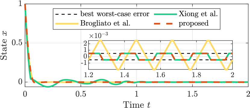
Figure 2: Results of the discrete-time STC without actuator saturation. Parameters: $k_{2}=10$, $k_{1}=27$.

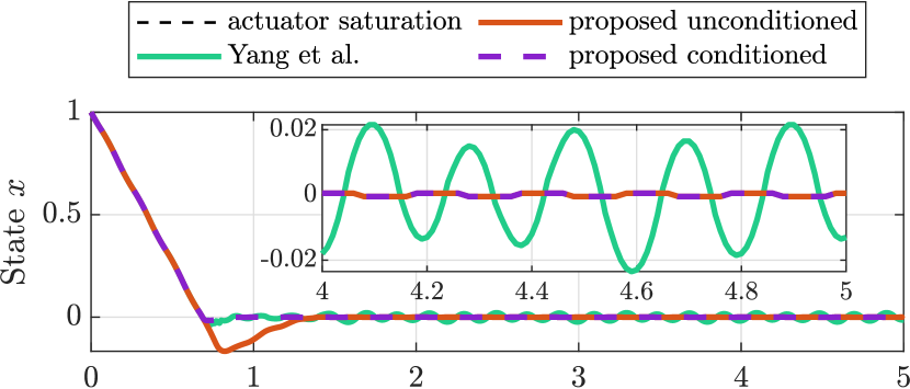
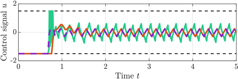
Figure 3: Results of the discrete-time STC in case of saturated actuation. Parameters: $k_{2}=10$, $k_{1}=16$, $U=1.5$. Top: plant state $x$, bottom: control signal $u$.

Fig. 3 shows the results of the discrete-time STC in the case of an actuator saturation. The saturation was set to $U=1.5$. The proposed algorithms are compared to the conditioned STC by Yang et al. (2023). The conditioned STC stops the integration within the controller state when it is in the saturation, which the unconditioned controller does not. This leads to a reduced convergence time of the conditioned controller compared to the unconditioned controller and to a largely reduced undershoot of the conditioned controller compared to the unconditioned STC. The conditioned controller by Yang et al. (2023) also stops the integration of the controller state, which leads to a reduced convergence time as well compared to the unconditioned controller. However, for the selected parameters $k_{2}=10$ and $k_{1}=16$, the conditioned controller by Yang et al. (2023) does not yield the same accuracy as the proposed controllers. This result contradicts (Yang et al., 2023, Theorem 1), and was already addressed in (Seeber, 2024) in a counterexample. Also, upon the zero-crossing of the state $x$, the control signal of the conditioned controller by Yang et al. (2023) exhibits a high-frequency switching behavior.

8 Conclusion

A new implicit discretization of the super-twisting controller was proposed. In contrast to existing approaches, the proposed controller can handle the same class of disturbances as its continuous-time counterpart while also achieving best possible worst-case performance and being intuitive to tune. For the case of constrained actuators, the proposed discretization was extended to the conditioned super-twisting controller. The resulting implicit conditioned super-twisting controller mitigates windup by means of the conditioning technique and features similarily simple stability conditions as its continuous-time counterpart. Numerical simulations demonstrated the superior performance of the proposed approach in comparison to existing approaches, as well as the proven stability and performance guarantees. Future work may study extensions of the proposed discretization to other higher order sliding-mode control laws.

Appendix A Proofs

The following auxiliary lemma is used in the proofs.

Lemma 21.

Let $Z\in\mathbb{R}_{>0}$ and $z_{k},z_{k+1}\in[-Z,Z]$. Suppose that $z_{k+1}\geq z_{k}$. Then, $\left\lfloor z_{k+1}\right\rceil^{\frac{1}{2}}\geq\left\lfloor z_{k}\right\rceil^{\frac{1}{2}}+\frac{z_{k+1}-z_{k}}{2\sqrt{Z}}.$

Proof A.1.

Let $\alpha_{k}=z_{k+1}-z_{k}\geq 0$ and define the function $h:\mathbb{R}_{\geq 0}\to\mathbb{R}$ as $h(\alpha)=\left\lfloor z_{k}+\alpha\right\rceil^{\frac{1}{2}}-\alpha/(2\sqrt{Z}).$ Then, for all $\alpha\in[0,\alpha_{k}]$ its derivative fulfills $\frac{\mathrm{d}{h}}{\mathrm{d}{\alpha}}\geq 0$, since $|z_{k}+\alpha|\leq Z$. Thus, $h(\alpha_{k})\geq h(0)$.

A.1 Proof of Proposition 1

For $M\in\mathbb{N}$, define an auxiliary Lipschitz continuous function $\eta_{M}:\mathbb{R}_{\geq 0}\to\mathbb{R}$ as

$$\eta_{M}(t)=\begin{cases}\eta(t)&\text{if $t\in[0,2M)$}\\ (-1)^{M}[1+(t-2M)]&\text{if $t\in[2M,2M+2)$}\\ 3(-1)^{M}&\text{if $t\in[2M+2,\infty)$}\end{cases}$$ (32)

with the sawtooth function $\eta$ defined as in (31). It is easy to verify that $\eta_{M}$ is Lipschitz continuous, and satisfies the inequalities $|\eta_{M}(t)|\leq 3$ and $|\dot{\eta}_{M}(t)|\leq 1$ almost everywhere. Moreover, $\int_{2\ell}^{2\ell+2}\eta(\tau)\,\mathrm{d}\tau=0$ holds for all integers $\ell\in[0,M-1]$ and $\int_{2M}^{2M+2}\eta_{M}(\tau)\,\mathrm{d}\tau=(-1)^{M}4$.

Now, define $w(t)=-\frac{qLT}{2}\eta_{K+1}(\frac{2t}{T})$ with $q\in\{-1,1\}$ to be specified. Then, $w_{k}=0$ for $k=0,\ldots,K$ regardless of $q$, and $w_{K+1}=(-1)^{K}qLT$ according to (3). Thus, $x_{0},\ldots,x_{K+1}$ and hence also $u_{0},\ldots,u_{K+1}$ are independent of $q$. Let

$$q=\begin{cases}(-1)^{K}&\text{if }2x_{K+1}-x_{K}+T(u_{K+1}-u_{K})\geq 0\\ (-1)^{K+1}&\text{otherwise}.\end{cases}$$ (33)

Then, (4) implies

$$x_{K+2} =2x_{K+1}-x_{K}+T(u_{K+1}-u_{K}+w_{K+1}-w_{K})$$

$$=\frac{(-1)^{K}}{q}(|2x_{K+1}-x_{K}+T(u_{K+1}-u_{K})|+LT^{2})$$ (34)

which yields $|x_{K+2}|\geq LT^{2}$, concluding the proof. ∎

A.2 Proof of Lemma 11

Substituting (12) into (11a) yields the generalized equation

$$z_{k+1}\in x_{k}-Tk_{1}\left\lfloor z_{k+1}\right\rceil^{\frac{1}{2}}-T^{2}k_{2}\left\lfloor z_{k+1}\right\rceil^{0}.$$ (35)

If $|x_{k}|\leq k_{2}T^{2}$, then its unique solution is $z_{k+1}=0$. Otherwise, $z_{k+1}$ and $x_{k}$ have the same sign, and multiplying (35) by $\operatorname{sign}(x_{k})=\operatorname{sign}(z_{k+1})$ yields the equation

$$|z_{k+1}|=|x_{k}|-Tk_{1}\left\lvert z_{k+1}\right\rvert^{\frac{1}{2}}-T^{2}k_{2}$$ (36)

whose unique solution is

$$\left\lvert z_{k+1}\right\rvert^{\frac{1}{2}} =-\frac{Tk_{1}}{2}+\sqrt{\frac{T^{2}k_{1}^{2}}{4}-T^{2}k_{2}+|x_{k}|}.$$ (37)

Substituting $k_{2}=\lambda+\frac{k_{1}^{2}}{4}$ yields (20). ∎

A.3 Proof of Lemma 13

Distinguish cases $|\hat{u}_{k}|\leq U$ and $|\hat{u}_{k}|>U$. In the first case, $\bar{u}_{k}=u_{k}=\hat{u}_{k}$, $z_{k+1}=\hat{z}_{k+1}$, $v_{k+1}=\hat{v}_{k+1}$ may be verified to be a solution of (11a), (17) by using (22). In the second case, suppose that $\hat{u}_{k}>U$; the proof for $\hat{u}_{k}<-U$ is obtained analogously. Set $u_{k}=U$, and let $v_{k+1}$, $\bar{u}_{k}$, and $z_{k+1}$ be uniquely defined by (17c), (17a), and (11a). It will be shown that $\bar{u}_{k}>U$, proving that also (17b) holds. To that end distinguish the two cases $\hat{v}_{k+1}\leq v_{k+1}$ and $\hat{v}_{k+1}>v_{k+1}$. In the first case,

$$z_{k+1}=x_{k}+T(u_{k}-v_{k+1})\leq x_{k}+T(\hat{u}_{k}-\hat{v}_{k+1})=\hat{z}_{k+1}$$ (38)

follows from (11a), (22a), and thus (17a), (22b) yield

$$\bar{u}_{k} =-k_{1}\left\lfloor z_{k+1}\right\rceil^{\frac{1}{2}}+2v_{k+1}-v_{k}$$

$$\geq-k_{1}\left\lfloor\hat{z}_{k+1}\right\rceil^{\frac{1}{2}}+2\hat{v}_{k+1}-v_{k}=\hat{u}_{k}>U.$$ (39)

For the second case, use (22b) and $\left\lfloor k_{1}\left\lfloor x\right\rceil^{\frac{1}{2}}\right\rceil^{0}=\left\lfloor x\right\rceil^{0}$ to rewrite (22c) as $\hat{v}_{k+1}\in v_{k}-Tk_{2}\left\lfloor 2\hat{v}_{k+1}-v_{k}-\hat{u}_{k}\right\rceil^{0}$, and note that the expression $\left\lfloor 2v_{k+1}-v_{k}-u_{k}\right\rceil^{0}$ in (17c) exceeds the one in that inclusion due to $\hat{v}_{k+1}>v_{k}$; hence

$$2v_{k+1}-v_{k}-u_{k}\geq 0\geq 2\hat{v}_{k+1}-v_{k}-\hat{u}_{k}$$ (40)

holds. Substituting (22b) yields $0\geq\hat{z}_{k+1}$, and (40) along with $\hat{v}_{k+1}>v_{k+1}$ further implies

$$u_{k}-v_{k+1}\leq v_{k+1}-v_{k}<\hat{v}_{k+1}-v_{k}\leq\hat{u}_{k}-\hat{v}_{k+1}.$$ (41)

Thus, $z_{k+1}<\hat{z}_{k+1}\leq 0$ is concluded as in (38). Then,

$$\bar{u}_{k}>2v_{k+1}-v_{k}\geq u_{k}=U$$ (42)

follows from (17a), (40), concluding the proof. ∎

A.4 Proof of Lemma 15

Define $Q_{T}(\mathbf{x})=\max_{\mathbf{h}\in\mathcal{F}(\mathbf{x})}V(\mathbf{x})-V(\mathbf{x}-T\mathbf{h})$, which is well-defined due to compactness of $\mathcal{F}(\mathbf{x})$ and continuity of $V$. To see upper semicontinuity, consider a sequence $(\mathbf{x}_{i})$ with limit $\bar{\mathbf{x}}$ and corresponding $\mathbf{h}_{i}\in\mathcal{F}(\mathbf{x}_{i})$ such that $Q_{T}(\mathbf{x}_{i})=V(\mathbf{x}_{i})-V(\mathbf{x}_{i}-T\mathbf{h}_{i})$ and $\lim_{i\to\infty}Q_{T}(\mathbf{x}_{i})=\limsup_{\mathbf{x}\to\bar{\mathbf{x}}}Q_{T}(\mathbf{x})$. Then, $\mathbf{h}_{i}$ converges to the compact set $\mathcal{F}(\bar{\mathbf{x}})$ due to upper semicontinuity of $\mathcal{F}$; thus, select subsequences such that $(\mathbf{h}_{i})$ converges to some $\bar{\mathbf{h}}\in\mathcal{F}(\bar{\mathbf{x}})$. Upper semicontinuity then follows from $\lim_{i\to\infty}Q_{T}(\mathbf{x}_{i})=V(\bar{\mathbf{x}})-V(\bar{\mathbf{x}}-T\bar{\mathbf{h}})\leq Q_{T}(\bar{\mathbf{x}})$.

To prove negative definiteness of $Q_{T}$, suppose to the contrary that there exist $\mathbf{x}\in\mathbb{R}^{n}\setminus\{\bm{0}\}$ and $\mathbf{h}\in\mathcal{F}(\mathbf{x})$ such that $V(\mathbf{x})-V(\mathbf{x}-T\mathbf{h})\geq 0$. Since $V$ is locally Lipschitz at $\mathbf{x}$, $\partial V(\mathbf{x})$ is nonempty and compact and $\partial V$ is upper semicontinuous at $\mathbf{x}$. Hence, $\bm{\zeta}\in\partial V(\mathbf{x})$ exists such that $\bm{\zeta}^{\mathrm{T}}(-T\mathbf{h})>0$. Since $V$ is quasiconvex, application of (Daniilidis and Hadjisavvas, 1999, Theorem 2.1) yields $V(\mathbf{x}-\lambda_{1}T\mathbf{h})\leq V(\mathbf{x}-\lambda_{2}T\mathbf{h})$ for all $0\leq\lambda_{1}\leq\lambda_{2}\leq 1$. Consequently, $V(\mathbf{x})=V(\mathbf{x}-\lambda T\mathbf{h})$ for all $\lambda\in[0,1]$, i.e., $V$ is constant on the line segment from $\mathbf{x}$ to $\mathbf{x}-T\mathbf{h}$. Thus, (Daniilidis and Hadjisavvas, 1999, Lemma 2.1) yields $\bm{\zeta}^{\mathrm{T}}\mathbf{h}=0$ for all $\bm{\zeta}\in\partial V(\mathbf{x}-\lambda T\mathbf{h})$ and all $\lambda\in(0,1)$. Choose any sequence $(\lambda_{i})$ tending to zero and converging $\bm{\zeta}_{i}\in\partial V(\mathbf{x}-\lambda_{i}T\mathbf{h})$. Due to upper semicontinuity of $\partial V$, then $\bar{\bm{\zeta}}=\lim_{i\to\infty}\bm{\zeta}_{i}\in\partial V(\mathbf{x})$, but $\bar{\bm{\zeta}}^{\mathrm{T}}\mathbf{h}=\lim_{i\to\infty}\bm{\zeta}_{i}^{\mathrm{T}}\mathbf{h}=0$, contradicting (26). ∎

A.5 Proof of Lemma 17

Continuity and positive definiteness of $V_{\alpha}$ as well as the fact that it is a strict Lyapunov function for (25) under the stated conditions are shown in (Seeber and Horn, 2017, Section 3). Local Lipschitz continuity outside the origin is obvious from the fact that the square root is zero only if $z=q=0$. From the definition of $V_{\alpha}$ and its continuity, one can see that $(z,q)\in\Omega_{\alpha,c}$ if and only if the inequalities $|12\alpha^{2}k_{1}^{2}z-2cq|\leq c^{2}-3q^{2}$, $|q|\leq\frac{c}{3}$ hold (cf. also Seeber and Horn, 2017, Fig. 1). Since both inequalities are convex in $(z,q)$, the set $\Omega_{\alpha,c}$ is convex by virtue of being the intersection of two convex sets. ∎

A.6 Proof of Lemma 18

For item (a), denote $\mathbf{x}=[z\quad q]^{\mathrm{T}}$ and define compact sets $\Lambda_{b}=\{\mathbf{x}\in\mathbb{R}^{2}:V_{\alpha}(\mathbf{x})\in[b,2b]\}$. For each $b>0$, existence of $\varepsilon_{b}>0$ will be shown such that $\mathbf{x}_{k+1}\in\Lambda_{b}$ implies $V_{\alpha}(\mathbf{x}_{k+1})\leq V_{\alpha}(\mathbf{x}_{k})-\varepsilon_{b}$, which implies finite-time attractivity and forward invariance of $\Omega_{\alpha,c}$. To that end, first relax (24) to $\mathbf{x}_{k+1}\in\mathbf{x}_{k}+T\mathcal{F}(\mathbf{x}_{k+1})$ with

$$\mathcal{F}(z,q)=\begin{bmatrix}-k_{1}\left\lfloor z\right\rceil^{\frac{1}{2}}+q\\ -k_{2}\left\lfloor z\right\rceil^{0}+[-L,L]\end{bmatrix}.$$ (43)

From Lemma 17, $V_{\alpha}$ is a strict Lyapunov function for $\dot{\mathbf{x}}\in\mathcal{F}(\mathbf{x})$, i.e., condition (26) of Lemma 15 is satisfied. Since also the other conditions of the latter lemma are fulfilled, $V_{\alpha}(\mathbf{x}_{k+1})-V_{\alpha}(\mathbf{x}_{k})\leq\max_{\mathbf{x}\in\Lambda_{b}}Q_{T}(\mathbf{x})=-\varepsilon_{b}$ holds whenever $\mathbf{x}_{k+1}\in\Lambda_{b}$; this maximum is well-defined due to upper semicontinuity of $Q_{T}$ and negative due to its negative definiteness. This proves item (a).

For item (b), choose $\alpha\in(0,1)$ sufficiently large such that $k_{1}>\frac{\sqrt{k_{2}+L}}{\alpha}$. Finite-time attractivity of $\Omega$ is then clear from the fact that it contains a finite-time attractive set $\Omega_{\alpha,c}$ with sufficiently small $c>0$. To show forward invariance of $\Omega$, it will be shown that $(z_{k+1},q_{k+1})\notin\Omega$ implies $(z_{k},q_{k})\notin\Omega$. Distinguish the cases $z_{k+1}\neq 0$ and $z_{k+1}=0$. In the first case, the contradiction

$$|z_{k} +Tq_{k}|$$

$$=|z_{k+1}+Tk_{1}\left\lfloor z_{k+1}\right\rceil^{\frac{1}{2}}+T^{2}k_{2}\operatorname{sign}(z_{k+1})-T^{2}\delta_{k+1}|$$

$$>(k_{2}-L)T^{2}.$$ (44)

is obtained by substituting $z_{k}$ and $q_{k}$ using (24). In the second case, $|z_{k+1}+Tq_{k+1}|>(k_{2}-L)T^{2}$ implies

$$|z_{k}| =|z_{k+1}-Tq_{k+1}+Tk_{1}\left\lfloor z_{k+1}\right\rceil^{\frac{1}{2}}|$$

$$=|Tq_{k+1}|>(k_{2}-L)T^{2}.$$ (45)

Finally, $(z_{k},q_{k})\in\Omega$ implies $z_{k+2}=q_{k+2}=0$, because then $(z_{k+1},q_{k+1})\in\Omega$, yielding $z_{k+2}=0$ as shown above, and thus $Tq_{k+2}=z_{k+2}+Tk_{1}\left\lfloor z_{k+2}\right\rceil^{\frac{1}{2}}-z_{k+1}=0$. ∎

A.7 Proof of Lemma 20

For item (a), it is first shown that $\mathcal{M}_{1}$ is forward invariant. This is seen from the fact that $|v_{k+1}|>U$ and $|v_{k}|\leq U$ imply the contradiction $|v_{k}|=|v_{k+1}+Tk_{2}\operatorname{sign}(v_{k+1})|>U$ from (17c), because $\operatorname{sign}(2v_{k+1}-v_{k}-u_{k})=\operatorname{sign}(v_{k+1})$. To show finite-time attractivity, note that $v_{k}$ cannot change sign without entering $\mathcal{M}_{1}$, because $U>k_{2}T$. Hence, without restriction of generality, it is sufficient to show that the assumption $v_{k}>U$ for all $k\in\mathbb{N}_{0}$ leads to a contradiction. Under this assumption, $v_{k}$ is strictly decreasing, because $v_{k+1}\geq v_{k}$ and (17c) imply the contradiction $v_{k+1}\leq v_{k}-k_{2}T$. Since $v_{k}$ is also bounded from below, there exists $\kappa\in\mathbb{N}$ such that $|v_{k+1}-v_{k}|\leq\frac{k_{2}T}{2}$ for all $k\geq\kappa$. Then, the right-hand side of (17c) is truly multivalued, i.e., $2v_{k+1}-v_{k}-u_{k}=0$. Thus, $0<U-\frac{k_{2}T}{2}\leq v_{k+1}+(v_{k+1}-v_{k})=u_{k}\leq\bar{u}_{k}$ and, using (11b), $z_{k}$ is seen to strictly increase according to

$$z_{k+1}-z_{k} =T(u_{k}+w_{k-1}-v_{k+1}+v_{k})$$ (46)

$$=T(v_{k+1}+w_{k+1})\geq T(U-W)\geq k_{2}T,$$

eventually leading to the contradiction $\bar{u}_{k}<0$ in (17a) for sufficiently large $k>\kappa$, proving item (a).

For item (b), since $\mathcal{M}_{2}\subset\mathcal{M}_{1}$ and due to item (a), it is sufficient to consider trajectories in $\mathcal{M}_{1}$, i.e., to assume $|v_{k}|\leq U$ for all $k$. Let $\varepsilon=\min\{\delta,U-W-k_{2}T\}$. It will be shown that $k_{1}^{2}z_{k+1}>(U+W+\delta)^{2}$ implies $z_{k}\geq z_{k+1}+\varepsilon T$, from which the claim follows due to $\varepsilon>0$ and symmetry reasons. Distinguish the cases $\bar{u}_{k}>U$, $\bar{u}_{k}<-U$, and $|\bar{u}_{k}|\leq U$. The first case cannot occur, because, using (17a) and $|v_{k+1}-v_{k}|\leq k_{2}T$, the contradiction

$$2W +k_{2}T<U+W<k_{1}\left\lfloor z_{k+1}\right\rceil^{\frac{1}{2}}=2v_{k+1}-v_{k}-\bar{u}_{k}$$

$$\quad<2v_{k+1}-v_{k}-U\leq v_{k+1}-v_{k}\leq k_{2}T$$ (47)

is obtained. In the second case, $u_{k}=-U$ and hence

$$z_{k} =z_{k+1}-T(u_{k}+w_{k-1}+v_{k}-v_{k+1})$$

$$\geq z_{k+1}-T(-U+W+k_{2}T)\geq z_{k+1}+T\varepsilon.$$ (48)

is obtained from (11b). And in the third case,

$$z_{k} =z_{k+1}-T(\bar{u}_{k}+w_{k-1}+v_{k}-v_{k+1})$$ (49)

$$=z_{k+1}-T(-k_{1}\left\lfloor z_{k+1}\right\rceil^{\frac{1}{2}}+w_{k-1}+v_{k+1})$$

$$\geq z_{k+1}+T(U+W+\delta-W-U)\geq z_{k+1}+T\varepsilon,$$

follows from $u_{k}=\bar{u}_{k}$ and (17a), proving item (b).

To show item (c), since $\mathcal{M}_{3}\subset\mathcal{M}_{2}$, it is again sufficient to consider trajectories in $\mathcal{M}_{2}$, i.e., to use the assumptions $k_{1}^{2}|z_{k}|\leq(U+W+\delta)^{2}$ and $|v_{k}|\leq U$ for all $k$. Let $\varepsilon=\frac{k_{1}^{2}}{2}\frac{U-W-k_{2}T}{U+W+\delta}-k_{2}>0$. It will be shown that $\bar{u}_{k}>U$ implies $\bar{u}_{k-1}\geq\bar{u}_{k}+T\varepsilon$; the claim then follows due to symmetry reasons. To see this, use $u_{k}=\operatorname{sat}_{U}(\bar{u}_{k})=U$ and (11b) to obtain $z_{k+1}\geq z_{k}+T(U-W-k_{2}T).$ Then, $\max\{\left\lvert z_{k}\right\rvert^{\frac{1}{2}},\left\lvert z_{k+1}\right\rvert^{\frac{1}{2}}\}\leq\frac{U+W+\delta}{k_{1}}$ and Lemma 21 imply

$$\left\lfloor z_{k+1}\right\rceil^{\frac{1}{2}} \geq\left\lfloor z_{k}\right\rceil^{\frac{1}{2}}+\frac{k_{1}T}{2}\frac{U-W-k_{2}T}{U+W+\delta}.$$ (50)

Thus, evaluating $\bar{u}_{k-1}$ and $\bar{u}_{k}$ using (17a) yields

$$\bar{u}_{k-1} =\bar{u}_{k}-k_{1}(\left\lfloor z_{k}\right\rceil^{\frac{1}{2}}-\left\lfloor z_{k+1}\right\rceil^{\frac{1}{2}})$$

$$\quad-2(v_{k+1}-v_{k})+(v_{k}-v_{k-1})$$

$$\geq\bar{u}_{k}+\frac{k_{1}^{2}T}{2}\frac{U-W-k_{2}T}{U+W+\delta}-k_{2}T$$

$$\quad-(v_{k+1}-v_{k})+(v_{k}-v_{k-1})$$

$$=\bar{u}_{k}+T\varepsilon+\gamma_{k}$$ (51)

with the abbreviation $\gamma_{k}=(v_{k}-v_{k-1})-(v_{k+1}-v_{k})$. Consequently, $\bar{u}_{k-1}\geq U-2k_{2}T$. Distinguish cases $v_{k-1}<U-2k_{2}T$ and $v_{k-1}\geq U-2k_{2}T$. In the first case, it will be shown that $v_{k}-v_{k-1}\geq k_{2}T$, which implies $\gamma_{k}\geq 0$ and allows to conclude $\bar{u}_{k-1}\geq\bar{u}_{k}+T\varepsilon$ from (51). To see this, suppose to the contrary that $v_{k}-v_{k-1}=ck_{2}T$ with some $c<1$. Then, $\bar{u}_{k-1}\geq U-(1-c)k_{2}T$ and $2v_{k}-v_{k-1}-u_{k-1}\geq 0$ follow from (51) and (17c), respectively. The former implies $u_{k-1}=\operatorname{sat}_{U}(\bar{u}_{k-1})\geq U-(1-c)k_{2}T$ and the latter yields $v_{k}\geq(u_{k-1}+v_{k-1})/2$, leading to the contradiction

$$v_{k}-v_{k-1} \geq\frac{u_{k-1}-v_{k-1}}{2}\geq\frac{-(1-c)k_{2}T+2k_{2}T}{2}$$

$$=\frac{1+c}{2}k_{2}T>ck_{2}T.$$ (52)

In the second case, the relation $\bar{u}_{k-1}\geq U-2k_{2}T$ implies $u_{k-1}\geq U-2k_{2}T$, and (18c) yields the inequality $v_{k}\geq\min\{v_{k-1},u_{k-1}\}\geq U-2k_{2}T$. Since $u_{k}=U$ and $u_{k-1},v_{k},v_{k-1}\in[U-2k_{2}T,U]$, one may conclude $|v_{k-1}-u_{k-1}|\leq 2k_{2}T$ and $|v_{k}-u_{k}|\leq 2k_{2}T$. By applying (18c) three times, $\gamma_{k}$ may then be bounded as

$$\gamma_{k} =\frac{u_{k-1}-v_{k-1}}{2}-\frac{u_{k}-v_{k}}{2}=\frac{u_{k-1}-U}{2}+\frac{v_{k}-v_{k-1}}{2}$$

$$=\frac{u_{k-1}-U}{2}+\frac{u_{k-1}-v_{k-1}}{4}\geq\frac{3}{4}(u_{k-1}-U).$$ (53)

If $u_{k-1}=U$, then $\gamma_{k}\geq 0$ and $\bar{u}_{k-1}\geq\bar{u}_{k}+T\varepsilon$ follows from (51). Otherwise, $u_{k-1}=\bar{u}_{k-1}$, leading to

$$\bar{u}_{k-1}\geq\bar{u}_{k}+T\varepsilon+\frac{3}{4}\bar{u}_{k-1}-\frac{3}{4}U\geq\frac{\bar{u}_{k}}{4}+T\varepsilon+\frac{3}{4}\bar{u}_{k-1}.$$ (54)

in (51); solving for $\bar{u}_{k-1}$ yields $\bar{u}_{k-1}\geq\bar{u}_{k}+4T\varepsilon$. ∎

References

• Acary and Brogliato (2010) Acary, V., Brogliato, B., 2010. Implicit Euler numerical scheme and chattering-free implementation of sliding mode systems. Sys. & Contr. Letters 59, 284–293.
• Andritsch et al. (2023) Andritsch, B., Watermann, L., Koch, S., Reichhartinger, M., Reger, J., Horn, M., 2023. Modified implicit discretization of the super-twisting controller arXiv:2303.15273.
• Bauschke and Combettes (2011) Bauschke, H.H., Combettes, P.L., 2011. Convex Analysis and Monotone Operator Theory in Hilbert Spaces. CMS Books in Mathematics. second ed., Springer.
• Brogliato (2023) Brogliato, B., 2023. Comments on “Finite-time stability of discrete autonomous systems”. Automatica 156, 111206.
• Brogliato et al. (2020) Brogliato, B., Polyakov, A., Efimov, D., 2020. The implicit discretization of the supertwisting sliding-mode control algorithm. IEEE Trans. on Automatic Control 65, 3707–3713.
• Daniilidis and Hadjisavvas (1999) Daniilidis, A., Hadjisavvas, N., 1999. Characterization of nonsmooth semistrictly quasiconvex and strictly quasiconvex functions. Journal of Optimization Theory and Applications 102, 525–536.
• Filippov (1988) Filippov, A.F., 1988. Differential Equations with Discontinuous Right-Hand Side. Kluwer.
• Haddad and Lee (2020) Haddad, W.M., Lee, J., 2020. Finite-time stability of discrete autonomous systems. Automatica 122, 109282.
• Hanan et al. (2021) Hanan, A., Levant, A., Jbara, A., 2021. Low-chattering discretization of sliding mode control, in: IEEE Conference on Decision and Control, pp. 6403–6408.
• Hanus et al. (1987) Hanus, R., Kinnaert, M., Henrotte, J.L., 1987. Conditioning technique, a general anti-windup and bumpless transfer method. Automatica 23, 729–739.
• Koch and Reichhartinger (2019) Koch, S., Reichhartinger, M., 2019. Discrete-time equivalents of the super-twisting algorithm. Automatica 107, 190–199.
• Levant (1993) Levant, A., 1993. Sliding order and sliding accuracy in sliding mode control. Int. Jnl. of Contr. 58, 1247–1263.
• Levant (2011) Levant, A., 2011. Discretization issues of high-order sliding modes, in: 18th IFAC World Con., pp. 1904–1909.
• Mojallizadeh et al. (2021) Mojallizadeh, M.R., Brogliato, B., Acary, V., 2021. Time-discretizations of differentiators: Design of implicit algorithms and comparative analysis. Int. Journal of Robust and Nonlinear Control 31, 7679–7723.
• Polyakov and Fridman (2014) Polyakov, A., Fridman, L., 2014. Stability notions and lyapunov functions for sliding mode control systems. Journal of the Franklin Institute 351, 1831–1865.
• Reichhartinger et al. (2023) Reichhartinger, M., Vogl, S., Koch, S., 2023. Anti-windup schemes for discrete-time super twisting algorithms, in: 22nd IFAC World Con., pp. 1609–1614.
• Seeber (2024) Seeber, R., 2024. Discussion on “Semi-implicit Euler digital implementation of conditioned super-twisting algorithm with actuation saturation”. IEEE Trans. on Industrial Electronics 71, 4304–4304.
• Seeber and Horn (2017) Seeber, R., Horn, M., 2017. Stability proof for a well-established super-twisting parameter setting. Automatica 84, 241–243.
• Seeber and Reichhartinger (2020) Seeber, R., Reichhartinger, M., 2020. Conditioned super-twisting algorithm for systems with saturated control action. Automatica 116, 108921.
• Shtessel et al. (2013) Shtessel, Y., Edwards, C., Fridman, L., Levant, A., 2013. Sliding Mode Control and Observation. Birkhauser.
• Xiong et al. (2022) Xiong, X., Chen, G., Lou, Y., Huang, R., Kamal, S., 2022. Discrete-time implementation of super-twisting control with semi-implicit Euler method. IEEE Trans. on Circuits and Systems II: Express Briefs 69, 99–103.
• Yang et al. (2023) Yang, X., Xiong, X., Zou, Z., Lou, Y., 2023. Semi-implicit Euler digital implementation of conditioned super-twisting algorithm with actuation saturation. IEEE Trans. on Industrial Electronics 70, 8388–8397.